A New Hybrid CQ Algorithm for the Split Feasibility Problem in Hilbert Spaces and Its Applications to Compressed Sensing

Abstract

In this paper, we focus on studying the split feasibility problem (SFP), which has many applications in signal processing and image reconstruction. A popular technique is to employ the iterative method which is so called the relaxed CQ algorithm. However, the speed of convergence usually depends on the way of selecting the step size of such algorithms. We aim to suggest a new hybrid CQ algorithm for the SFP by using the self adaptive and the line-search techniques. There is no computation on the inverse and the spectral radius of a matrix. We then prove the weak convergence theorem under mild conditions. Numerical experiments are included to illustrate its performance in compressed sensing. Some comparisons are also given to show the efficiency with other CQ methods in the literature.

1. Introduction

In the present work, we aim to study the split feasibility problem (SFP), which is to find a point

$$x^{*}\in C\mathrm{such}\mathrm{that}A{x}^{*}\in Q$$

(1)

where C and Q are nonempty closed and convex subsets of real Hilbert spaces $H_1$ and $H_2$, respectively, and $A:H_1\to H_2$ a bounded linear operator. In 1994, the SFP was first investigated by Censor and Elfving [1] in finite dimensional Hilbert spaces. There have been applications in real world such as image processing and signal recovery (see [2,3]). Byrne [4,5] introduced the following recursive procedure for solving SFP:

$$x_{n+1}=P_C(x_n-{\alpha }_n{A}^{*}(I-P_Q)A{x}_n)$$

(2)

where $\left\{{\alpha }_n\right\}\subset (0,2/{\parallel A\parallel }^2)$, $P_C$ and $P_Q$ are the projections onto C and Q, respectively, and $A^{*}$ is the adjoint of A. This projection algorithm is usually called the CQ algorithm. Subsequently, Yang [6] introduced the relaxed CQ algorithm. In this case, the projections $P_C$ and $P_Q$ are, respectively, replaced by $P_{C_n}$ and $P_{Q_n}$, where

$$C_n=\{x\in H_1:c\left(x_n\right)+⟨{\xi }_n,x-x_n⟩\le 0\},$$

(3)

where $c:H_1\to \mathbb{R}$ is convex and lower semicontinuous, and ${\xi }_n\in \partial c\left(x_n\right)$, and

$$Q_n=\{y\in H_2:q\left(A{x}_n\right)+⟨{\eta }_n,y-A{x}_n⟩\le 0\},$$

(4)

where $q:H_2\to \mathbb{R}$ is convex and lower semicontinuous, and ${\eta }_n\in \partial q\left(A{x}_n\right).$ In what follows, we define

$$f_n\left(x\right)=\frac{1}{2}{\parallel (I-P_{Q_n})Ax\parallel }^2,n\ge 1$$

(5)

and

$$\nabla f_n\left(x\right)=A^{*}(I-P_{Q_n})Ax.$$

(6)

Precisely, Yang [6] proposed the relaxed CQ algorithm in a finite-dimensional Hilbert space as follows:

Algorithm 1.

Let$x_1\in H_1$. For$n\ge 1$, define

$$x_{n+1}=P_{C_n}(x_n-{\alpha }_n\nabla f_n\left(x_n\right)).$$

(7)

where$\left\{{\alpha }_n\right\}\subset (0,2/{\parallel A\parallel }^2).$

It is seen that, since the sets $C_n$ and $Q_n$ are half spaces, the projections are easily to be computed. However, the step size $\left\{{\alpha }_n\right\}$ still depends on the norm of A.

To eliminate this difficulty, in 2012, López et al. [7] suggested a new way to select the step size ${\alpha }_n$ as follows:

$${\alpha }_n=\frac{{\beta }_n{f}_n\left(x_n\right)}{\parallel \nabla f_n\left(x_n\right){\parallel }^2}$$

(8)

where $\left\{{\beta }_n\right\}$ is a sequence in $(0,4)$ such that $0<a\le {lim\; inf}_{n\to \infty }{\beta }_n\le {lim\; sup}_{n\to \infty }{\beta }_n\le b<4$ for some $a,b\in (0,4)$. They established the weak convergence of the CQ algorithm (Equation (2)) and the relaxed CQ algorithm (Equation (7)) with the step size defined by Equation (8) in real Hilbert spaces.

Qu and Xiu [8] adopted the line-search technique to construct the step size in Euclidean spaces as follows:

Algorithm 2.

Choose$\sigma >0$, $\rho \in (0,1)$, $\mu \in (0,1)$. Let$x_1$be a point in$H_1$. For$n\ge 1$, let

$$y_n=P_{C_n}(x_n-{\alpha }_n\nabla f_n\left(x_n\right)),$$

(9)

where${\alpha }_n=\sigma {\rho }^{m_n}$and$m_n$is the smallest nonnegative integer such that

$${\alpha }_n\parallel \nabla f_n\left(x_n\right)-\nabla f_n\left(y_n\right)\parallel \le \mu \parallel x_n-y_n\parallel .$$

(10)

Set

$$x_{n+1}=P_{C_n}(x_n-{\alpha }_n\nabla f_n\left(y_n\right)).$$

(11)

In 2012, Bnouhachem et al. [9] proposed the following projection method for solving the SFP.

Algorithm 3.

For a given$x_1\in {\mathbb{R}}^n$, let

$$y_n=P_{C_n}(x_n-{\alpha }_n\nabla f_n\left(x_n\right))$$

(12)

where${\alpha }_n>0$satisfies

$${\alpha }_n\parallel \nabla f_n\left(x_n\right)-\nabla f_n\left(y_n\right)\parallel \le \mu \parallel x_n-y_n\parallel ,0<\mu <1.$$

(13)

Define

$$x_{n+1}=P_{C_n}(x_n-{\phi }_{n}d(x_n,{\alpha }_n))$$

(14)

where

$$\begin{array}{ccc}\hfill d(x_n,{\alpha }_n)& =& x_n-y_n+{\alpha }_n\nabla f_n\left(y_n\right)\hfill \\ \hfill {\epsilon }_n& =& {\alpha }_n(\nabla f_n\left(y_n\right)-\nabla f_n\left(x_n\right))\hfill \\ \hfill D(x_n,{\alpha }_n)& =& x_n-y_n-{\epsilon }_n\hfill \\ \hfill \varphi (x_n,{\alpha }_n)& =& ⟨x_n-y_n,D(x_n,{\alpha }_n)⟩\hfill \end{array}$$

(15)

and

$${\phi }_n=\frac{\varphi (x_n,{\alpha }_n)}{\parallel d(x_n,{\alpha }_n){\parallel }^2}.$$

(16)

Recently, many authors establish weak and strong convergence theorems for the SFP (see also [10,11]).

In this work, combining the work of Bnouhachem et al. [9] and López et al. [7], we suggest a new hybrid CQ algorithm for solving the split feasibility problem and establish weak convergence theorem in Hilbert spaces. Finally, numerical results are given for supporting our main results. The comparison is also given to algorithms of Qu and Xiu [8] and Bnouhachem et al. [9]. It is shown that our method has a better convergence behavior than these CQ algorithms through numerical examples.

2. Preliminaries

We next recall some useful basic concepts that will be used in our proof. Let H be a real Hilbert space equipped with the inner product $⟨·,·⟩$ and the norm $\parallel ·\parallel$. Let $T:H\to H$ be a nonlinear mapping. Then, T is called firmly nonexpansive if, for all $x,y\in H$,

$$⟨x-y,Tx-Ty⟩\ge {\parallel Tx-Ty\parallel }^2.$$

(17)

In a real Hilbert space H, we have the following equality:

$$⟨x,y⟩=\frac{1}{2}{\parallel x\parallel }^2+\frac{1}{2}{\parallel y\parallel }^2-\frac{1}{2}{\parallel x-y\parallel }^2.$$

(18)

A function $f:H\to \mathbb{R}$ is convex if and only if

$$f\left(z\right)\ge f\left(x\right)+⟨\nabla f\left(x\right),z-x⟩$$

(19)

for all $z\in H$.

A function $f:H\to \mathbb{R}$ is said to be weakly lower semi-continuous (w-lsc) at x if $x_n\rightharpoonup x$ implies

$${\displaystyle f\left(x\right)\le \underset{n\to \infty }{lim\; inf}f\left(x_n\right).}$$

(20)

The projection of a nonempty, closed and convex set C onto H is defined by

$${\displaystyle P_{C}x:=arg\underset{y\in C}{min}{\parallel x-y\parallel }^2,x\in H.}$$

(21)

We note that $P_C$ and $I-P_C$ are firmly nonexpansive. From [5], we know that, if

$${\displaystyle f\left(x\right)=\frac{1}{2}{\parallel (I-P_Q)Ax\parallel }^2,}$$

then $\nabla f$ is ${\parallel A\parallel }^2$-Lipschitz continuous. Moreover, in real Hilbert spaces, we know that [12]

(i)

$⟨x-P_{C}x,z-P_{C}x⟩\le 0$ for all $z\in C$;

(ii)

${\parallel P_{C}x-P_{C}y\parallel }^2\le ⟨P_{C}x-P_{C}y,x-y⟩$ for all $x,y\in H$; and

(iii)

${\parallel P_{C}x-z\parallel }^2\le {\parallel x-z\parallel }^2-{\parallel P_{C}x-x\parallel }^2$ for all $z\in C$.

Lemma 1.

[12] Let S be a nonempty, closed and convex subset of a real Hilbert space H and $\left\{x_n\right\}$ be a sequence in H that satisfies the following assumptions:

(i) 

${\displaystyle \underset{n\to \infty }{lim}\parallel x_n-x\parallel }$ exists for each $x\in S$; and

(ii) 

${\omega }_w\left(x_n\right)\subset S$.

Then, $\left\{x_n\right\}$ converges weakly to a point in S.

3. Main Results

Throughout this paper, let S be the set of solution of SFP and suppose that S is nonempty. Let C and Q be nonempty that satisfy the following assumptions:

(A1) The set C is defined by

$$C=\{x\in H_1:c\left(x\right)\le 0\},$$

(22)

where $c:H_1\to \mathbb{R}$ is convex, subdifferentiable on C and bounded on bounded sets, and the set Q is defined by

$$Q=\{y\in H_2:q\left(y\right)\le 0\},$$

(23)

where $q:H_2\to \mathbb{R}$ is convex, subdifferentiable on Q and bounded on bounded sets.

(A2) For each $x\in H_1$, at least one subgradient $\xi \in \partial c\left(x\right)$ can be computed, where

$$\partial c\left(x\right)=\{z\in H_1:c\left(u\right)\ge c\left(x\right)+⟨u-x,z⟩,\forall u\in H_1\}.$$

(24)

(A3) For each $y\in H_2$, at least one subgradient $\eta \in \partial q\left(y\right)$ can be computed, where

$$\partial q\left(x\right)=\{w\in H_2:q\left(u\right)\ge q\left(y\right)+⟨v-y,w⟩,\forall v\in H_2\}.$$

(25)

Next, we propose our new relaxed CQ algorithm in real Hilbert spaces.

Algorithm 4.

Let$x_1\in H_1$, for any$\sigma >0, \rho \in (0,1)$, $\mu \in (0,\frac{1}{2})$. Assume$\left\{x_n\right\}$and$\left\{y_n\right\}$have been constructed. Compute$x_{n+1}$via the formula

$$y_n=P_{C_n}(x_n-{\alpha }_n\nabla f_n\left(x_n\right)),$$

(26)

where${\alpha }_n=\sigma {\rho }^{m_n}$and$m_n$is the smallest nonnegative integer such that

$${\alpha }_n\parallel \nabla f_n\left(x_n\right)-\nabla f_n\left(y_n\right)\parallel \le \mu \parallel x_n-y_n\parallel .$$

(27)

Define

$$x_{n+1}=y_n-{\tau }_n\nabla f_n\left(y_n\right)$$

(28)

where

$${\tau }_n=\frac{{\beta }_n{f}_n\left(y_n\right)}{\parallel \nabla f_n\left(y_n\right){\parallel }^2+{\theta }_n},0<{\beta }_n<4,0<{\theta }_n<1.$$

(29)

Lemma 2.

[8] The line-search in Equation (27) terminates after a finite number of steps. In addition, we have the following:

$${\displaystyle \frac{\mu \rho }{L}<{\alpha }_n\le \sigma }$$

(30)

for all $n\ge 1$, where $L={\parallel A\parallel }^2$.

Next, we state our main theorem in this paper.

Theorem 1.

Assume that $\left\{{\theta }_n\right\}$ and $\left\{{\beta }_n\right\}$ satisfy the assumptions:

(a1) 

${\displaystyle \underset{n\to \infty }{lim}{\theta }_n=0}$; and

(a2) 

${\displaystyle \underset{n\to \infty }{lim\; inf}{\beta }_n(4-{\beta }_n)>0}$.

Then, $\left\{x_n\right\}$ defined by Algorithm 4 converges weakly to a solution of the SFP.

Proof. 

Let $z\in S$. Then, we have $z=P_{C_n}\left(z\right)$ and $Az=P_{Q_n}\left(Az\right)$. It follows that $\nabla f_n\left(z\right)=0$. We see that

$$\begin{array}{ccc}\hfill {\parallel x_{n+1}-z\parallel }^2& =& {\parallel y_n-{\tau }_n\nabla f_n\left(y_n\right)-z\parallel }^2\hfill \\ & =& {\parallel y_n-z\parallel }^2+{\tau }_n^2{\parallel \nabla f_n\left(y_n\right)\parallel }^2-2{\tau }_n⟨y_n-z,\nabla f_n\left(y_n\right)⟩.\hfill \end{array}$$

(31)

Since $I-P_{Q_n}$ is firmly nonexpansive and $\nabla f_n\left(z\right)=0$, we get

$$\begin{array}{ccc}\hfill ⟨y_n-z,\nabla f_n\left(y_n\right)⟩& =& ⟨y_n-z,\nabla f_n\left(y_n\right)-\nabla f_n\left(z\right)⟩\hfill \\ & =& ⟨y_n-z,A^{*}(I-P_{Q_n})A{y}_n-A^{*}(I-P_{Q_n})Az⟩\hfill \\ & =& ⟨A{y}_n-Az,(I-P_{Q_n})A{y}_n-(I-P_{Q_n})Az⟩\hfill \\ & \ge & {\parallel (I-P_{Q_n})A{y}_n\parallel }^2\hfill \\ & =& 2f_n\left(y_n\right).\hfill \end{array}$$

(32)

It also follows that

$$⟨x_n-z,\nabla f_n\left(x_n\right)⟩\ge 2f_n\left(x_n\right).$$

(33)

From Equation (19), we see that

$$\begin{array}{ccc}\hfill 2{\alpha }_n⟨y_n-x_n,\nabla f_n\left(x_n\right)⟩& =& 2{\alpha }_n⟨y_n-x_n,\nabla f_n\left(x_n\right)-\nabla f_n\left(y_n\right)⟩+2{\alpha }_n⟨y_n-x_n,\nabla f_n\left(y_n\right)⟩\hfill \\ & \ge & -2{\alpha }_n\parallel y_n-x_n\parallel \parallel \nabla f_n\left(x_n\right)-\nabla f_n\left(y_n\right)\parallel \hfill \\ & & +2{\alpha }_n\frac{1}{2}(\parallel (I-P_{Q_n})A{y}_n{\parallel }^2-\parallel (I-P_{Q_n})A{x}_n{\parallel }^2)\hfill \\ & \ge & -2{\alpha }_n\parallel y_n-x_n\parallel \parallel \nabla f_n\left(x_n\right)-\nabla f_n\left(y_n\right)\parallel -2{\alpha }_n{f}_n\left(x_n\right).\hfill \end{array}$$

(34)

From Equations (33) and (34), we obtain

$$\begin{array}{ccc}\hfill {\parallel y_n-z\parallel }^2& =& {\parallel P_{C_n}(x_n-{\alpha }_n\nabla f_n\left(x_n\right))-z\parallel }^2\hfill \\ & \le & {\parallel x_n-{\alpha }_n\nabla f_n\left(x_n\right)-z\parallel }^2-{\parallel y_n-x_n+{\alpha }_n\nabla f_n\left(x_n\right)\parallel }^2\hfill \\ & =& \parallel x_n{-z\parallel }^2+{\parallel {\alpha }_n\nabla f_n\left(x_n\right)\parallel }^2-2{\alpha }_n⟨x_n-z,\nabla f_n\left(x_n\right)⟩\hfill \\ & & -{\parallel y_n-x_n\parallel }^2-{\parallel {\alpha }_n\nabla f_n\left(x_n\right)\parallel }^2-2{\alpha }_n⟨y_n-x_n,\nabla f_n\left(x_n\right)⟩\hfill \\ & =& {\parallel x_n-z\parallel }^2-2{\alpha }_n⟨x_n-z,\nabla f_n\left(x_n\right)⟩-{\parallel y_n-x_n\parallel }^2-2{\alpha }_n⟨y_n-x_n,\nabla f_n\left(x_n\right)⟩\hfill \\ & \le & {\parallel x_n-z\parallel }^2-4{\alpha }_n{f}_n\left(x_n\right)-{\parallel y_n-x_n\parallel }^2\hfill \\ & & +2{\alpha }_n\parallel y_n-x_n\parallel \parallel \nabla f_n\left(x_n\right)-\nabla f_n\left(y_n\right)\parallel +2{\alpha }_n{f}_n\left(x_n\right)\hfill \\ & \le & {\parallel x_n-z\parallel }^2-2{\alpha }_n{f}_n\left(x_n\right)-\parallel y_n-x_n{\parallel }^2+2\mu {\parallel y_n-x_n\parallel }^2\hfill \\ & =& {\parallel x_n-z\parallel }^2-2{\alpha }_n{f}_n\left(x_n\right)-(1-2\mu ){\parallel y_n-x_n\parallel }^2.\hfill \end{array}$$

(35)

Combining Equations (31), (32) and (35), we get

$$\begin{array}{ccc}\hfill {\parallel x_{n+1}-z\parallel }^2& \le & {\parallel x_n-z\parallel }^2-2{\alpha }_n{f}_n\left(x_n\right)-(1-2\mu )\parallel y_n-x_n{\parallel }^2+{\tau }_n^2{\parallel \nabla f_n\left(y_n\right)\parallel }^2-4{\tau }_n{f}_n\left(y_n\right)\hfill \\ & =& {\parallel x_n-z\parallel }^2-2{\alpha }_n{f}_n\left(x_n\right)-(1-2\mu ){\parallel y_n-x_n\parallel }^2\hfill \\ & & +\frac{{\beta }_n^2{f}_n^2\left(y_n\right)}{(\parallel \nabla f_n\left(y_n\right){{\parallel }^2+{\theta }_n)}^2}{\parallel \nabla f_n\left(y_n\right)\parallel }^2-\frac{4{\beta }_n{f}_n^2\left(y_n\right)}{\parallel \nabla f_n\left(y_n\right){\parallel }^2+{\theta }_n}\hfill \\ & \le & {\parallel x_n-z\parallel }^2-2{\alpha }_n{f}_n\left(x_n\right)-(1-2\mu ){\parallel y_n-x_n\parallel }^2\hfill \\ & & +\frac{{\beta }_n^2{f}_n^2\left(y_n\right)}{\parallel \nabla f_n\left(y_n\right){\parallel }^2+{\theta }_n}-\frac{4{\beta }_n{f}_n^2\left(y_n\right)}{\parallel \nabla f_n\left(y_n\right){\parallel }^2+{\theta }_n}\hfill \\ & =& {\parallel x_n-z\parallel }^2-2{\alpha }_n{f}_n\left(x_n\right)-(1-2\mu ){\parallel y_n-x_n\parallel }^2\hfill \\ & & -{\beta }_n(4-{\beta }_n)\frac{f_n^2\left(y_n\right)}{\parallel \nabla f_n\left(y_n\right){\parallel }^2+{\theta }_n}\hfill \\ & \le & {\parallel x_n-z\parallel }^2-2\frac{\mu \ell }{L}{f}_n\left(x_n\right)-(1-2\mu ){\parallel y_n-x_n\parallel }^2\hfill \\ & & -{\beta }_n(4-{\beta }_n)\frac{f_n^2\left(y_n\right)}{\parallel \nabla f_n\left(y_n\right){\parallel }^2+{\theta }_n},\hfill \end{array}$$

(36)

where the last inequality follows from Lemma 2. Since $0<{\beta }_n<4$ and ${\displaystyle 0<\mu <\frac{1}{2}}$, it follows that

$$\parallel x_{n+1}-z\parallel \le \parallel x_n-z\parallel .$$

(37)

Thus, ${\displaystyle \underset{n\to \infty }{lim}\parallel x_n-z\parallel }$ exists and hence $\left\{x_n\right\}$ is bounded.

From Equation (36) and Assumption (A2), it also follows that

$$\underset{n\to \infty }{lim}\frac{f_n^2\left(y_n\right)}{\parallel \nabla f_n\left(y_n\right){\parallel }^2+{\theta }_n}=0.$$

(38)

By Assumption (A1), we have

$$\underset{n\to \infty }{lim}\frac{f_n^2\left(y_n\right)}{\parallel \nabla f_n\left(y_n\right){\parallel }^2}=0.$$

(39)

It follows that

$$\underset{n\to \infty }{lim}{f}_n\left(y_n\right)=\underset{n\to \infty }{lim}\parallel (I-P_{Q_n})A{y}_n\parallel =0,$$

(40)

and

$$\underset{n\to \infty }{lim}{f}_n\left(x_n\right)=\underset{n\to \infty }{lim}\parallel (I-P_{Q_n})A{x}_n\parallel =0.$$

(41)

From Equation (36), we have

$$\underset{n\to \infty }{lim}\parallel y_n-x_n\parallel =0.$$

(42)

Using Equations (40) and (42), we have

$$\begin{array}{ccc}\hfill \parallel A{x}_n-P_{Q_n}A{y}_n\parallel & =& \parallel A{x}_n-A{y}_n+A{y}_n-P_{Q_n}A{y}_n\parallel \hfill \\ & \le & \parallel A{x}_n-A{y}_n\parallel +\parallel A{y}_n-P_{Q_n}A{y}_n\parallel \hfill \\ & =& \parallel A\parallel \parallel x_n-y_n\parallel +\parallel A{y}_n-P_{Q_n}A{y}_n\parallel \hfill \\ & \to & 0\mathrm{as}n\to \infty .\hfill \end{array}$$

(43)

Let $x^{*}$ be a cluster point of $\left\{x_n\right\}$ with $\left\{x_{n_k}\right\}$ converging to $x^{*}$. From Equation (42), we see that $\left\{y_{n_k}\right\}$ also converges to $x^{*}$. We next show that $x^{*}$ is in S. Since $y_{n_k}\in C_{n_k}$, by the definition of $C_{n_k}$, we have

$$c\left(x_{n_k}\right)+⟨{\xi }_{n_k},y_{n_k}-x_{n_k}⟩\le 0$$

(44)

where ${\xi }_{n_k}\in \partial c\left(x_{n_k}\right)$. By the assumption that $\left\{{\xi }_{n_k}\right\}$ is bounded and Equation (42), we get

$$\begin{array}{ccc}\hfill c\left(x_{n_k}\right)& \le & ⟨{\xi }_{n_k},x_{n_k}-y_{n_k}⟩\hfill \\ & \le & \parallel {\xi }_{n_k}\parallel \parallel x_{n_k}-y_{n_k}\parallel \hfill \\ & \to & 0\mathrm{as}k\to \infty \hfill \end{array}$$

(45)

which implies $c\left(x^{*}\right)\le 0$. Hence $x^{*}\in C$. Since $P_{Q_{n_k}}\left(A{y}_{n_k}\right)\in Q_{n_k}$, we obtain

$$q\left(A{x}_{n_k}\right)+⟨{\eta }_{n_k},P_{Q_{n_k}}A{y}_{n_k}-A{x}_{n_k}⟩\le 0$$

(46)

where ${\eta }_{n_k}\in \partial q\left(A{x}_{n_k}\right)$. By the boundedness of $\left\{{\eta }_{n_k}\right\}$ and Equation (43), it follows that

$$\begin{array}{ccc}\hfill q\left(A{x}_{n_k}\right)& \le & ⟨{\eta }_{n_k},A{x}_{n_k}-P_{Q_{n_k}}A{y}_{n_k}⟩\hfill \\ & \le & \parallel {\eta }_{n_k}\parallel \parallel A{x}_{n_k}-P_{Q_{n_k}}A{y}_{n_k}\parallel \hfill \\ & \to & 0\mathrm{as}k\to \infty .\hfill \end{array}$$

(47)

We conclude that $q\left(A{x}^{*}\right)\le 0$. Thus, $A{x}^{*}\in Q$. Thus, $x^{*}$ is a solution of the SFP.

Hence, by Lemma 1, we conclude that the sequence $\left\{x_n\right\}$ converges to a point in S. This completes the proof. □

4. Numerical Experiments

In this section, we provide numerical experiments in compressed sensing. We illustrate the performance of Algorithms 4 and 1 of Yang [6], Algorithm 2 of Qu and Xiu [8], and Algorithm 3 of Bnouhuchem et al. [9]. In signal processing, compressed sensing can be modeled as the following linear equation:

$$y=Ax+\epsilon ,$$

(48)

where $x\in {\mathbb{R}}^N$ is a recovered vector with m nonzero components, $y\in {\mathbb{R}}^M$ is the observed data, $\epsilon$ is the noisy and A is an $M\times N$ matrix with $M<N$. The problem in Equation (48) can be seen as the LASSO problem:

$${\displaystyle \underset{x\in {\mathbb{R}}^N}{min}\frac{1}{2}{\parallel y-Ax\parallel }^2\mathrm{subject}\mathrm{to}{\parallel x\parallel }_1\le t,}$$

(49)

where $t>0$ is a given constant. In particular, if $C=\{x\in {\mathbb{R}}^N:{\parallel x\parallel }_1\le t\}$ and $Q=\left\{y\right\}$, then the LASSO problem can be considered as the SFP. From this connection, we can apply the CQ algorithm to solve Equation (49).

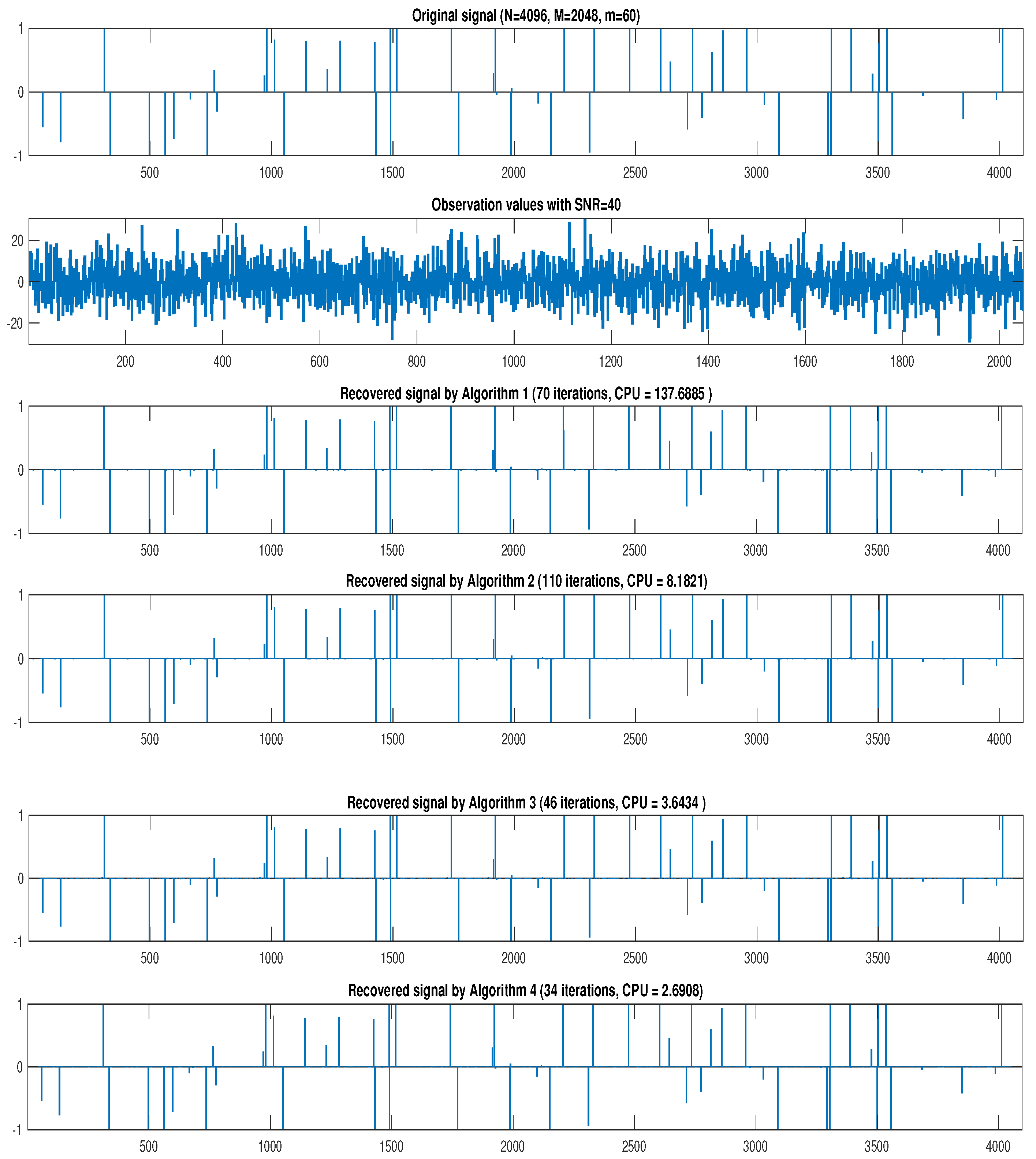
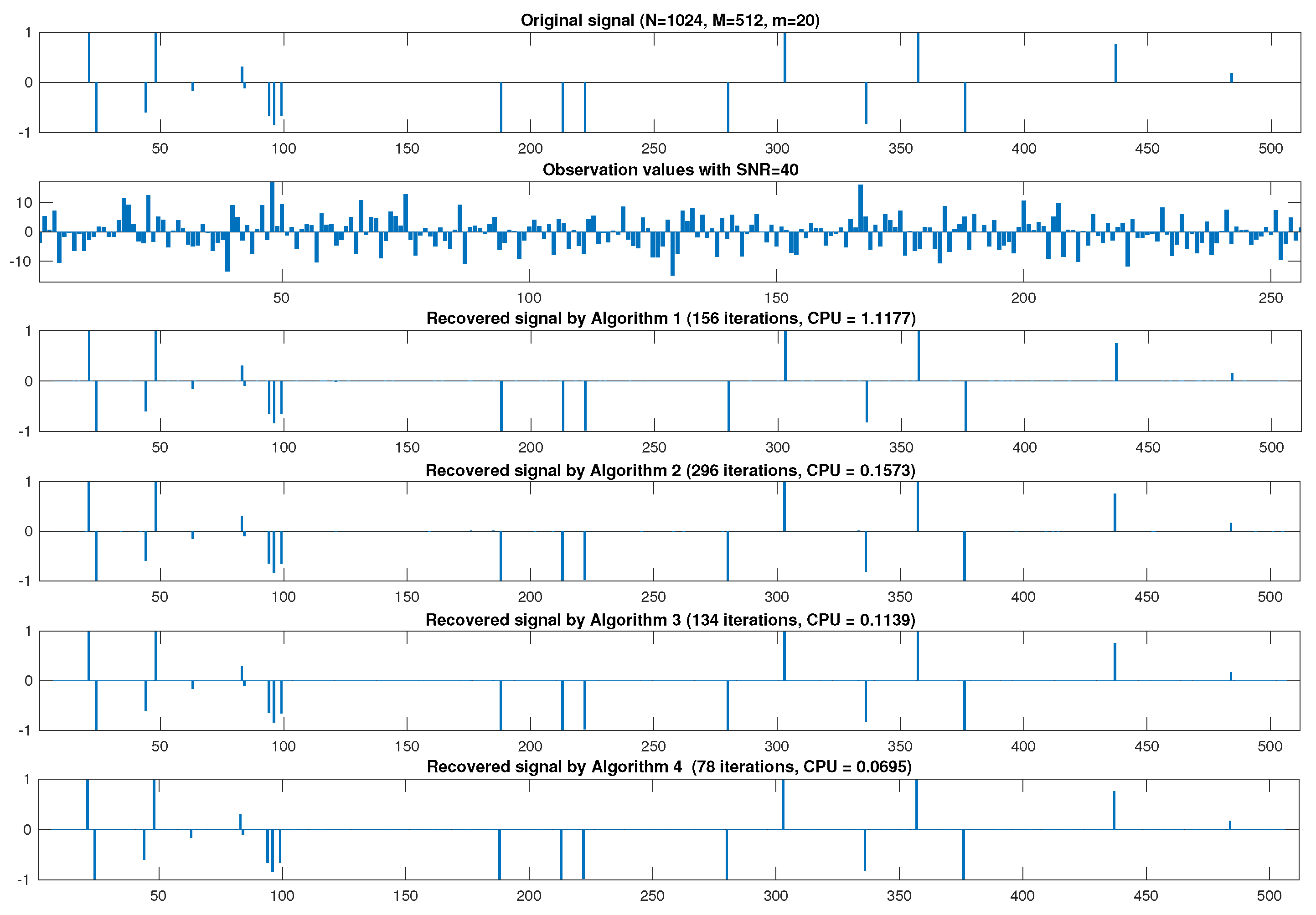
In this example, the sparse vector $x\in {\mathbb{R}}^N$ is generated by the uniform distribution in $[-2,2]$ with m nonzero elements. The matrix A is generated by the normal distribution with mean zero and invariance one. The observation y is generated by the white Gaussian noise with SNR=40. The process is started with $t=m$ and initial point $x_1=ones(N,1)$.

The stopping criterion is defined by the mean square error (MSE):

$${\displaystyle E_n=\frac{1}{N}{\parallel x_n-x^{*}\parallel }^2<\kappa ,}$$

(50)

where $x_n$ is an estimated signal of $x^{*}$ and $\kappa$ is a tolerance.

In what follows, let $\mu =0.3$, $\sigma =0.2$, $\rho =0.4$, ${\beta }_n=1.9$ and ${\displaystyle {\theta }_n=\frac{1}{200n+1}}$. The numerical results are reported as follows.

In Table 1, we observe that the performance of Algorithm 4 is better than other algorithms in terms of CPU time and number of iterations as the spikes of sparse vector is varied from 10 to 30. In this example, it is shown that Algorithm 4 of Yang [6], for which the step size depends on the norm of A, converges more slowly than other algorithms in terms of CPU time.

Table 1. Numerical results ($M=512$ and $N=1024$).

m-Sparse	Method	$\mathit{\kappa }={10}^{-4}$		$\mathit{\kappa }={10}^{-5}$
		CPU	Iter	CPU	Iter
$m=10$	Algorithm 1	0.7801	93	0.5931	83
	Algorithm 2	0.0962	187	0.1000	158
	Algorithm 3	0.1416	257	0.0605	74
	Algorithm 4	0.0271	33	0.0592	39
$m=15$	Algorithm 1	0.6345	93	0.6778	101
	Algorithm 2	0.1020	196	0.1001	195
	Algorithm 3	0.1087	170	0.0823	97
	Algorithm 4	0.0251	35	0.0430	51
$m=20$	Algorithm 1	1.1535	161	1.1177	156
	Algorithm 2	0.1661	308	0.1573	296
	Algorithm 3	0.3557	500	0.1139	134
	Algorithm 4	0.0516	55	0.0695	78
$m=25$	Algorithm 1	0.7380	103	2.9774	443
	Algorithm 2	0.0990	196	0.4746	940
	Algorithm 3	0.0623	115	0.7258	1308
	Algorithm 4	0.0354	42	0.0922	165
$m=30$	Algorithm 1	1.1423	168	3.7280	92
	Algorithm 2	0.1568	321	1.7980	666
	Algorithm 3	0.1219	164	0.4119	111
	Algorithm 4	0.0704	70	0.1335	38

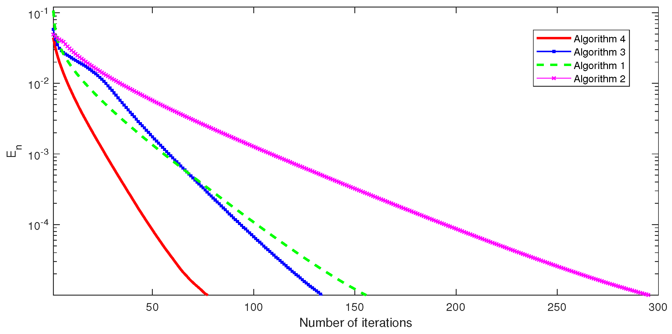
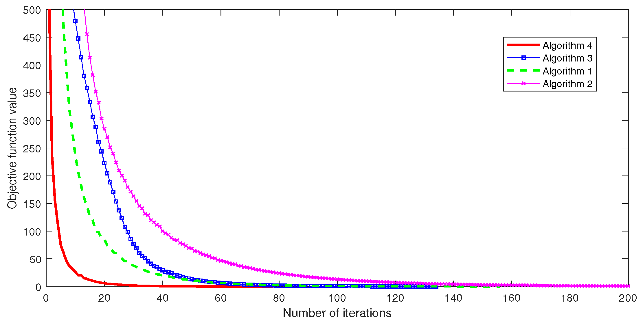
Next, we provide Figure 1, Figure 2 and Figure 3 to illustrate the convergence behavior, MSE, number of iterations and objective function values when $N=1024$, $M=512$, $m=20$ and $\kappa ={10}^{-5}$.

Figure 1. From top to bottom: original signal, observation data and recovered signal by Algorithms 1–4, respectively.

Figure 2. MSE versus number of iterations when $N=1024$, $M=512$ and $\kappa ={10}^{-5}$.

Figure 3. The objective function value versus number of iterations when $N=1024$, $M=512$ and $\kappa ={10}^{-5}$.

In Figure 1, Figure 2 and Figure 3, we can summarize that our proposed algorithm is really more efficient and faster than algorithms of Yang [6], Qu and Xiu [8] and Bnouhachem et al. [9].

In Table 2, we observe that Algorithm 4 is effective and also converges more quickly than Algorithm 1 of Yang [6], Algorithm 2 of Qu and Xiu [8] and Algorithm 3 of Bnouhuchem et al. [9]. Moreover, it is seen that Algorithm 1 of Yang [6] has the highest CPU time in computation. In this case, Algorithm 1 takes more CPU time than it does in the first case (see Table 1). Therefore, we can conclude that our proposed method has the advantage in comparison to other methods, especially Algorithm 1, which requires the spectral computation.

Table 2. Numerical results ($M=2048$ and $N=4096$).

m-sparse	Method	$\mathit{\kappa }={10}^{-4}$		$\mathit{\kappa }={10}^{-5}$
		CPU	Iter	CPU	Iter
$m=20$	Algorithm 1	53.4863	28	77.8192	40
	Algorithm 2	3.1953	43	4.7627	62
	Algorithm 3	1.5285	19	2.3102	28
	Algorithm 4	1.0771	13	1.6199	20
$m=40$	Algorithm 1	74.6456	38	106.3420	54
	Algorithm 2	4.5607	60	6.1862	83
	Algorithm 3	2.0701	26	2.9406	37
	Algorithm 4	1.4418	18	2.1713	27
$m=60$	Algorithm 1	86.1752	45	137.6885	70
	Algorithm 2	5.2204	70	8.1821	110
	Algorithm 3	2.3965	30	3.6434	46
	Algorithm 4	1.7580	22	2.6908	34
$m=80$	Algorithm 1	133.5504	67	219.4587	112
	Algorithm 2	7.8185	104	13.3599	178
	Algorithm 3	3.4220	43	5.9392	75
	Algorithm 4	2.4207	30	3.7902	47
$m=100$	Algorithm 1	148.3098	75	327.4775	163
	Algorithm 2	8.7840	118	19.7221	258
	Algorithm 3	3.8024	48	16.0518	202
	Algorithm 4	2.6962	34	5.3538	66

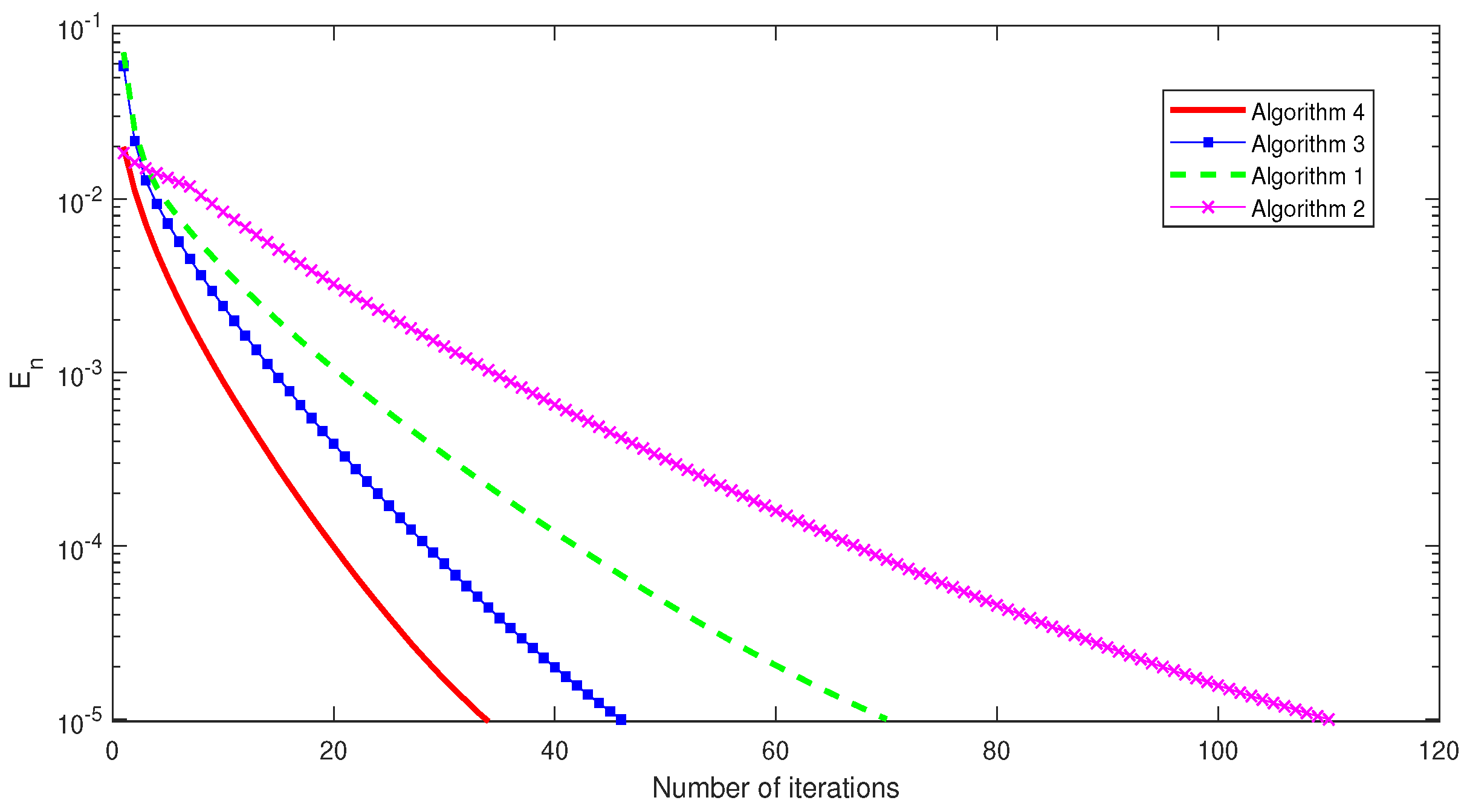
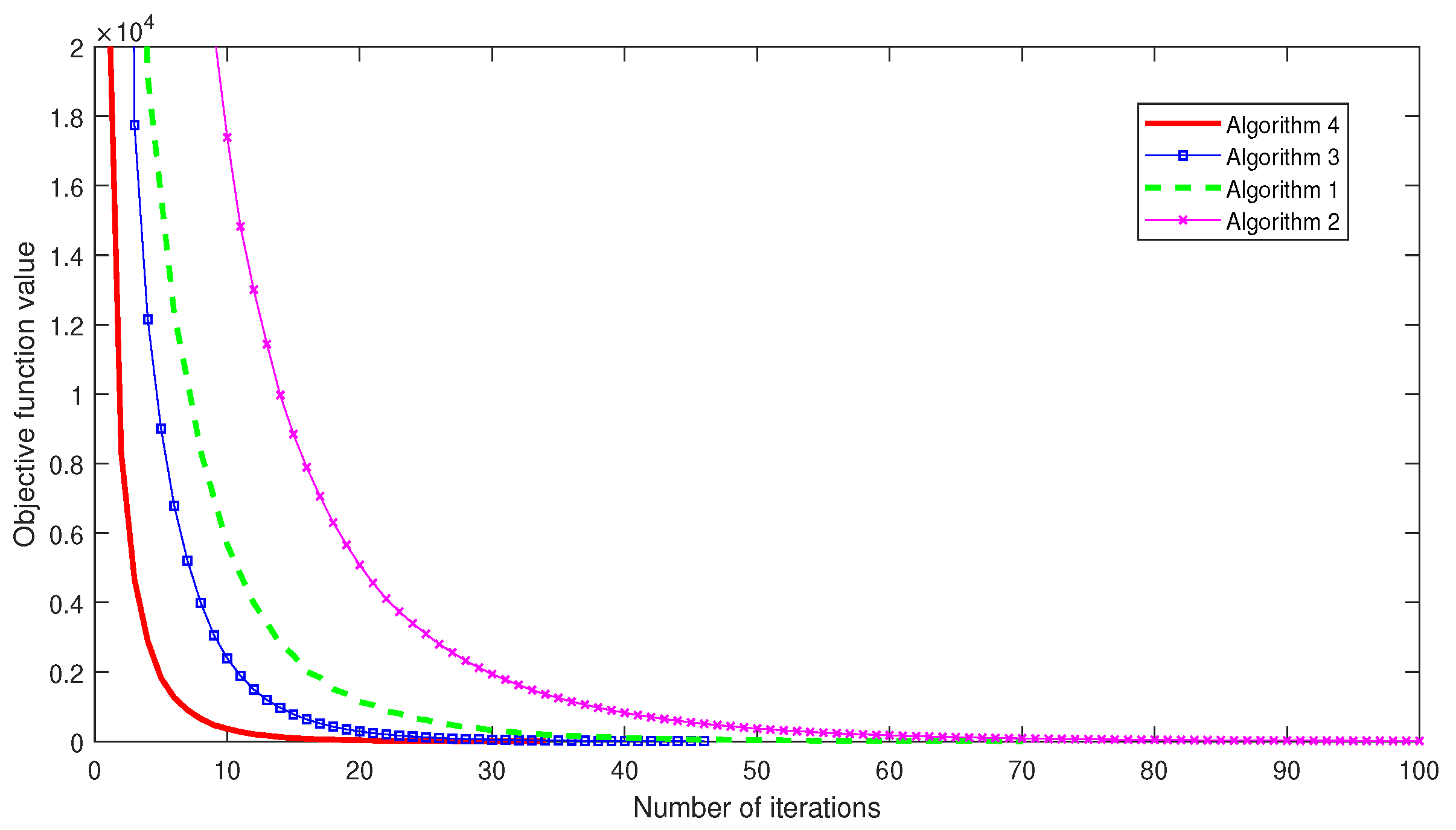
We next provide Figure 4, Figure 5 and Figure 6 to illustrate the convergence behavior, MSE, number of iterations and objective function values when $N=4096$, $M=2048$, $m=60$ and $\kappa ={10}^{-5}$.

Figure 4. From top to bottom: original signal, observation data and recovered signal by Algorithms 1–4, respectively.

Figure 5. MSE versus number of iterations when $N=4096$, $M=2048$ and $\kappa ={10}^{-5}$.

Figure 6. The objective function value versus number of iterations when $N=4096$, $M=2048$ and $\kappa ={10}^{-5}$.

In Figure 4, Figure 5 and Figure 6, we observe that MSE and objective function values of Algorithm 4 decreases faster than Algorithms 1–3 do in each cases.

5. Comparative Analysis

In this section, we discuss the comparative analysis to show the effects of the step sizes ${\alpha }_n$ and ${\beta }_n$ in Algorithm 4.

We begin this section by studying the effect of the step size ${\beta }_n$ in Algorithm 4 in terms of the number of iterations and the CPU time with the varied cases.

Choose $\mu =0.3$, $\sigma =0.2$, $\rho =0.4$ and ${\theta }_n=\frac{1}{200n+1}$. Let $x_1$ and A be as in the previous example. The stopping criterion is defined by Equation (50) with $\kappa ={10}^{-5}$.

In Table 3, it is observed that the number of iterations and the CPU time have small reduction when the step size ${\beta }_n$ tends to 4. The numerical experiments for each cases of ${\beta }_n$ are shown in Figure 7 and Figure 8, respectively.

Table 3. The convergence behavior of Algorithm 4 with different cases of ${\beta }_n$.

	${\mathit{\beta }}_{\mathit{n}}$	CPU	Iter
N = 1024	0.1	0.4585	139
M = 512	0.5	0.1976	73
m = 20	1.0	0.1632	55
	1.5	0.1272	44
	2.0	0.1187	38
	2.5	0.1048	35
	3.0	0.1065	32
	3.5	0.1298	29
	3.9	0.0954	28
N = 4096	0.1	4.4547	58
M = 2048	0.5	3.6075	39
m = 20	1.0	2.2021	29
	1.5	1.8119	24
	2.0	1.6024	21
	2.5	1.5748	29
	3.0	1.4055	17
	3.5	1.3297	16
	3.9	1.3172	15

Figure 7. Graph of number of iterations versus $E_n$ in case $N=1024$ and $M=512$.

Figure 8. Graph of number of iterations versus $E_n$ in case $N=4096$ and $M=2048$.

Next, we discuss the effect of the step size ${\alpha }_n$ in Algorithm 4. We note that the step size ${\alpha }_n$ depends on the parameters $\rho$ and $\sigma$. Thus, we aim to vary these parameters and study its convergence behavior.

Choose $\mu =0.3$, $\sigma =0.2$, ${\beta }_n=3.9$ and ${\theta }_n=\frac{1}{200n+1}$. Let $x_1$ and A be as in the previous example. The stopping criterion is defined by Equation (50) with $\kappa ={10}^{-5}$. The numerical results are reported in Table 4.

Table 4. The convergence behavior of Algorithm 4 with different cases of $\rho$.

	$\mathit{\rho }$	CPU	Iter
N = 1024	0.1	0.0634	27
M = 512	0.3	0.0981	26
m = 20	0.5	0.1065	26
	0.7	0.1773	27
	0.9	0.5421	27
N = 4096	0.1	0.7554	17
M = 2048	0.3	1.2094	17
m = 20	0.5	1.7697	17
	0.7	3.1876	17
	0.9	10.1536	18

In Table 4, we see that the CPU time decreases significantly when the parameter $\rho$ is also decreased. However, the choice of $\rho$ has no effect in terms of number of iterations.

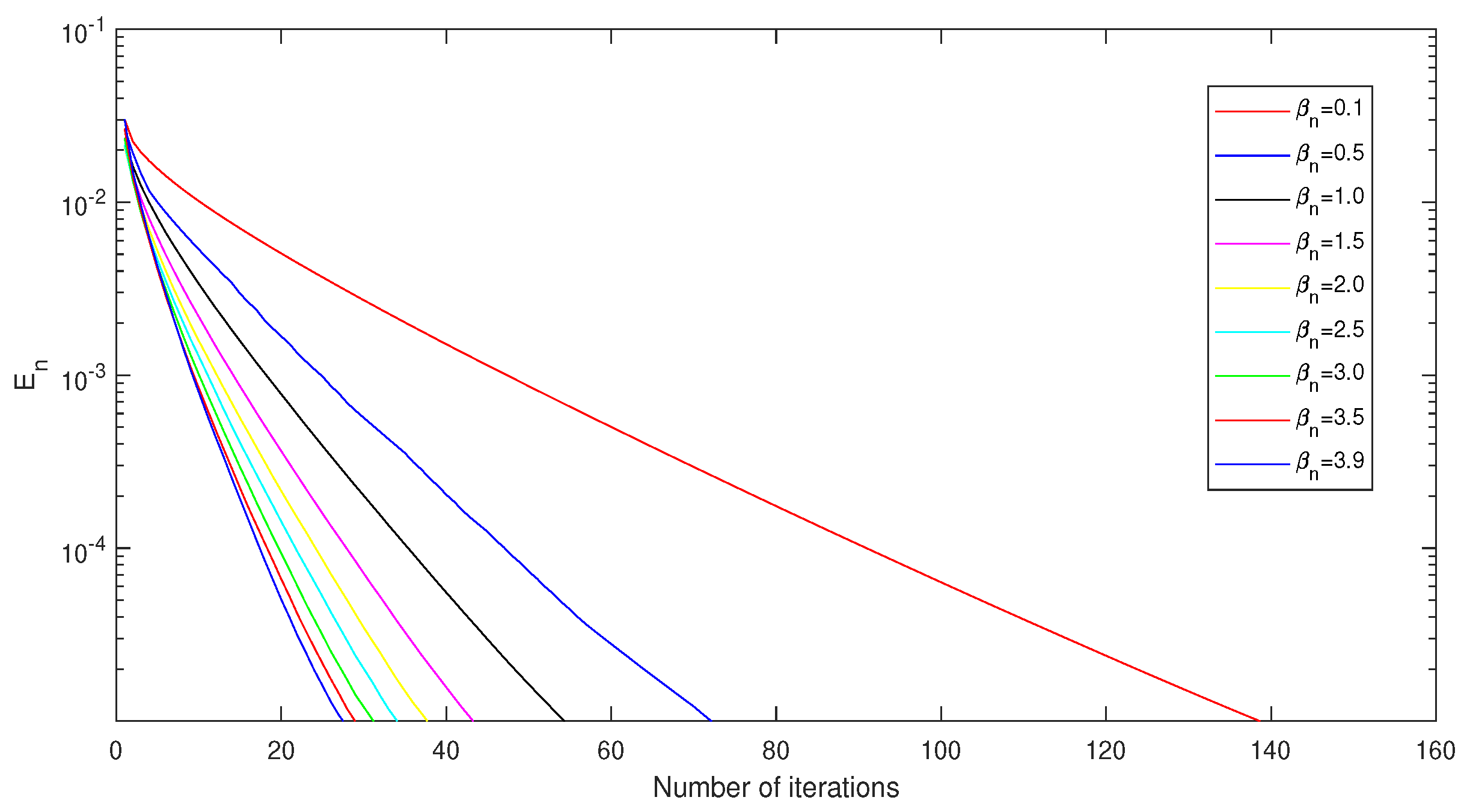
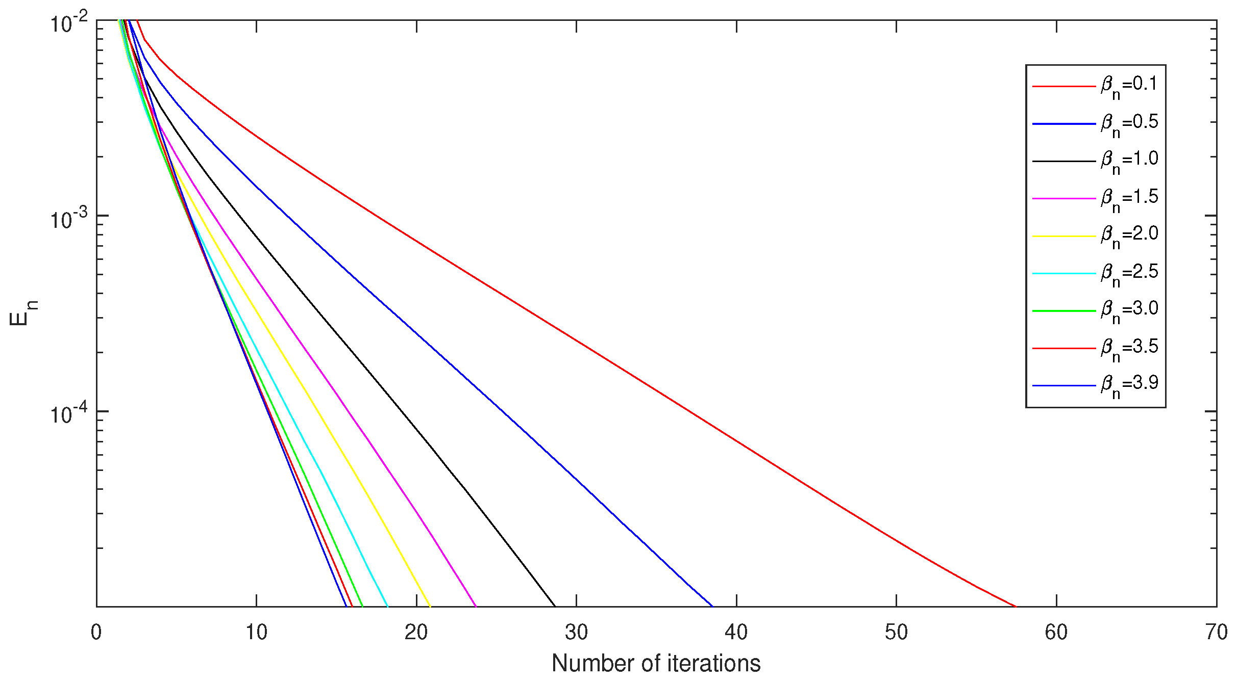
Next, we discuss the effect of $\sigma$ in Algorithm 4. In this experiment, choose $\mu =0.3$, ${\beta }_n=3.9$, $\rho =0.5$ and ${\theta }_n=\frac{1}{200n+1}$. The error $E_n$ is defined by Equation (50) with $\kappa ={10}^{-5}$. The numerical results are reported in Table 5.

Table 5. The convergence behavior Algorithm 4 with different cases of $\sigma$.

	$\mathit{\sigma }$	CPU	Iter
N = 1024	1	0.2985	53
M = 512	2	0.2974	53
m = 20	3	0.2636	56
	4	0.2478	53
	5	0.2584	52
	6	0.2816	56
N = 4096	1	1.9105	16
M = 2048	2	1.9990	16
m = 20	3	2.0937	16
	4	2.1371	16
	5	2.2449	17
	6	2.3816	16

In Table 5, we observe that the choices of $\sigma$ have a small effect in both terms of the CPU time and the number of iterations.

Finally, we discuss the convergence of Algorithm 4 with different cases of M and N. In this case, we set $\sigma =1$, $\rho =0.5$, $\mu =0.3$, ${\beta }_n=3.9$ and ${\theta }_n=\frac{1}{200n+1}$. The stopping criterion is defined by Equation (50).

In Table 6, it is shown that, if M and N have a high value, then the number of iteration decreases. However, in this case, the CPU time increases.

Table 6. The convergence behavior Algorithm 4 with different cases of M and N.

	$\mathit{\kappa }={10}^{-4}$		$\mathit{\kappa }={10}^{-5}$
	CPU	Iter	CPU	Iter
$M=1024$	0.9967	13	1.4998	21
$N=2048$
$M=2048$	3.8625	11	5.6119	16
$N=4096$
$M=3072$	5.0449	6	6.5788	8
$N=6144$
$M=4096$	7.3689	5	10.1838	7
$N=8192$

6. Conclusions

In this work, we introduce a new hybrid CQ algorithm by using the self adaptive and the line-search techniques for the split feasibility problem in Hilbert spaces. This method can be viewed as a refinement and improvement of other CQ algorithms. Convergence analysis of the proposed method is proved under some suitable conditions. The numerical results show that our algorithm has a better convergence behavior than the algorithms of Yang [6], Qu and Xiu [8] and Bnouhachem et al. [9]. A comparative analysis was also performed to show the effects of the step sizes in our algorithm.