The Mittag-Leffler Fitting of the Phillips Curve

Abstract

In this paper, a mathematical model based on the one-parameter Mittag-Leffler function is proposed to be used for the first time to describe the relation between the unemployment rate and the inflation rate, also known as the Phillips curve. The Phillips curve is in the literature often represented by an exponential-like shape. On the other hand, Phillips in his fundamental paper used a power function in the model definition. Considering that the ordinary as well as generalised Mittag-Leffler function behave between a purely exponential function and a power function it is natural to implement it in the definition of the model used to describe the relation between the data representing the Phillips curve. For the modelling purposes the data of two different European economies, France and Switzerland, were used and an “out-of-sample” forecast was done to compare the performance of the Mittag-Leffler model to the performance of the power-type and exponential-type model. The results demonstrate that the ability of the Mittag-Leffler function to fit data that manifest signs of stretched exponentials, oscillations or even damped oscillations can be of use when describing economic relations and phenomenons, such as the Phillips curve.

1. Introduction

It is because of, or thanks to, Paul Anthony Samuelson and Robert Merton Solow [1], that the economists all around the world call the negative correlation between the rate of wage change (or the price inflation rate) and the unemployment rate the Phillips curve (PC). It is lesser-known that the idea occurred in the work by Irving Fisher [2] more than 30 years before publishing the famous paper of Alban William Housego Phillips [3]. Fisher was not the only one who would deserve such an important discovery be named after him. Three years before Phillips paper, Arthur Joseph Brown [4] precisely described the inverse relation between the wage and price inflation and the rate of unemployment. Also Richard George Lipsey [5] played an important role by the birth, creation of the theoretical foundations and popularisation of the PC. In the empirical studies the inverse relationship between the rate of wage change and the unemployment rate was proven, e.g., for the United States of America [1,6,7] or United Kingdom [3,4,5]. The policy implications were for the first time mentioned by Samuelson and Solow [1]. The PC was in its beginnings widely used by the policy-makers to benefit from the trade-off to decrease the unemployment at a cost of minor increase of the inflation–the “sacrifice ratio”. Since then the PC has been studied, extended and re-formulated by many authors. For example, the model representing the New Keynesian theory of the output-inflation trade-off allows the expectations to jump based on the current and anticipated changes in policy. The new Keynesian Phillips curve (NKPC) model uses the ideas coming from the models of staggered contracts [8,9] and the quadratic price adjustment cost model of Rotemberg and Woodford [10], all of which have a similar formulation as the expectations-augmented PC of Friedman and Phelps [11,12]. The work of Clarida et al. [13] illustrates the widely usage of this model in theoretical analysis of monetary policy. Shifting the focus from the unemployment rate to the output gap, the Phillips’ relationship has become an aggregate supply curve. The NKPC stayed popular also in the late 1990s and at the beginning of the 21st century as a theory for understanding inflation dynamics (e.g., [14]).

When Magnus Gustaf Mittag-Leffler, in his works [15,16] proposed a new function $E_{\alpha }\left(x\right)$, he surely did not expect how important generalisation of the exponential function $e^x$ he developed. The Mittag-Leffler (ML) function and its generalisations interpolate between a purely exponential law and a power-law-like behaviour, and they arise naturally in the solution of fractional-order integro-differential equations, random walks, Lévy flights, the study of complex systems, and in other fields. In numerous works the properties, generalisations and applications of the ML-type functions were studied e.g., [17,18,19,20,21,22,23,24,25,26], and computation procedures for evaluating the ML function were developed e.g., [27,28,29]. The ML function become of great use and importance not only for mathematicians, but thanks to its special properties and huge potential for solving applied problems it found its applicability also in the fields such as psychorheology [19], electrotechnics [30,31], modeling of processes (diffusion [32], combustion [33], universe expansion [34]), etc. The ML function is also widely used in the numerical methods for solving ordinary and partial fractional-order differential equations, and in the the field of “fractal calculus” [35]. The idea to use the fractional-order calculus and the ML function for modelling phenomenons from the fields of economics and econophysics was elaborated by several authors [36,37,38,39,40,41,42].

In this paper the one-parameter ML function is for the first time used to model the relation between the unemployment rate and the inflation rate - the Phillips curve, and its performance is compared to the power-type model and the exponential-type model. French and Swiss econometric data are taken for the period of time 1980–2017 from the portal EconStats^TM [43] to identify the PC of these economies. The dataset is split into two subsets, the “modelling” subset is used to identify the model parameters, and a shorter “out-of-sample” subset serves for evaluating the forecast-performance of the models. The performance of all three models is evaluated based on the fitting-criterion, i.e., the sum of squared errors (SSE). The results are presented in the form of figures and tables, where the SSE of the fitting curve to the “modelling” subset, SSE of the fitting curve to the “out-of-sample” subset, and SSE of the fitting curve to the complete dataset, as well as some other quality criterions for the goodness-of-fit are listed.

The paper is organised as follows. Section 2 gives an overview of Mittag-Leffler function and its generalisations. The original Phillips curve as well as the Mittag-Leffler model for fitting the Phillips curve is described in Section 3. The numerical results and the discussion on the experiments can be found in Section 4. Finally, concluding remarks are given in Section 5.

2. Preliminaries: Mittag-Leffler Function and Its Generalisations

In 1903 M. G. Mittag-Leffler [15,16] introduced a new function $E_{\alpha }\left(x\right)$, a generalisation of the classical exponential function $e^x$, which is till today known as the one-parameter ML function. Using Erdélyi’s notation [44], where z is used instead of x, the function can be written as:

$$\begin{array}{c}\hfill E_{\alpha }\left(z\right)=\sum _{k=0}^{\infty }\frac{z^k}{\mathsf{\Gamma }(\alpha k+1)},\alpha \in \mathbb{C},Re\left(\alpha \right)>0,z\in \mathbb{C},\end{array}$$

(1)

where $\mathsf{\Gamma }$ denotes the (complete) Gamma function, having the property $\mathsf{\Gamma }\left(n\right)=(n-1)!$. The one-parameter ML function and its properties were further investigated [45,46,47,48] followed by the generalisation to a two-parameter function of the ML-type, by some authors called the Wiman’s function (some give the credit to Agarwal). Following the Erdélyi’s handbook the formula has the form [44]:

$$\begin{array}{c}\hfill E_{\alpha ,\beta }\left(z\right)=\sum _{k=0}^{\infty }\frac{z^k}{\mathsf{\Gamma }(\alpha k+\beta )},\alpha ,\beta \in \mathbb{C},Re\left(\alpha \right)>0,Re\left(\beta \right)>0,z\in \mathbb{C}.\end{array}$$

(2)

The main properties of the above mentioned functions, and other ML-type functions, can be found in the book by Erdélyi et al. [44], and a detailed overview in the book by Dzhrbashyan [17]. To demonstrate the concept of generality of the ML-type functions let us point out, that the ML function for one parameter (1), is a special case of the two-parameter ML function, i.e., if we substitute $\beta =1$ in (2). Accordingly, the classical exponential function is a special case of the one-parameter ML function, where $\alpha =1$:

$$\begin{array}{c}\hfill E_{\alpha ,1}\left(z\right)=\sum _{k=0}^{\infty }\frac{z^k}{\mathsf{\Gamma }(\alpha k+1)}\equiv E_{\alpha }\left(z\right),\\ \hfill \\ \hfill E_1\left(z\right)=\sum _{k=0}^{\infty }\frac{z^k}{\mathsf{\Gamma }(k+1)}=\sum _{k=0}^{\infty }\frac{z^k}{k!}=e^z.\end{array}$$

Also, other authors introduced and investigated further generalisations of the ML function, but as these are not used in the following experiments, they are not discussed in details here.

3. Modelling the Phillips Curve

As in many fields of science and applications, so in economics, to describe a relation between two variables, regression analysis is often used. One can use different regression models from simple linear-type, throughout exponential- and power-type models, to polynomial ones, and many other more complex and sophisticated. The discussion on the linearity or nonlinearity, and on the convex or concave shape of the PC, if it is supposed to be nonlinear, is still ongoing. Some authors are in favour of convex shape [49,50,51,52], some of concave [53], and some of their combination [54]. The application of the ML-type function to describe the PC perfectly fits into this discussion.

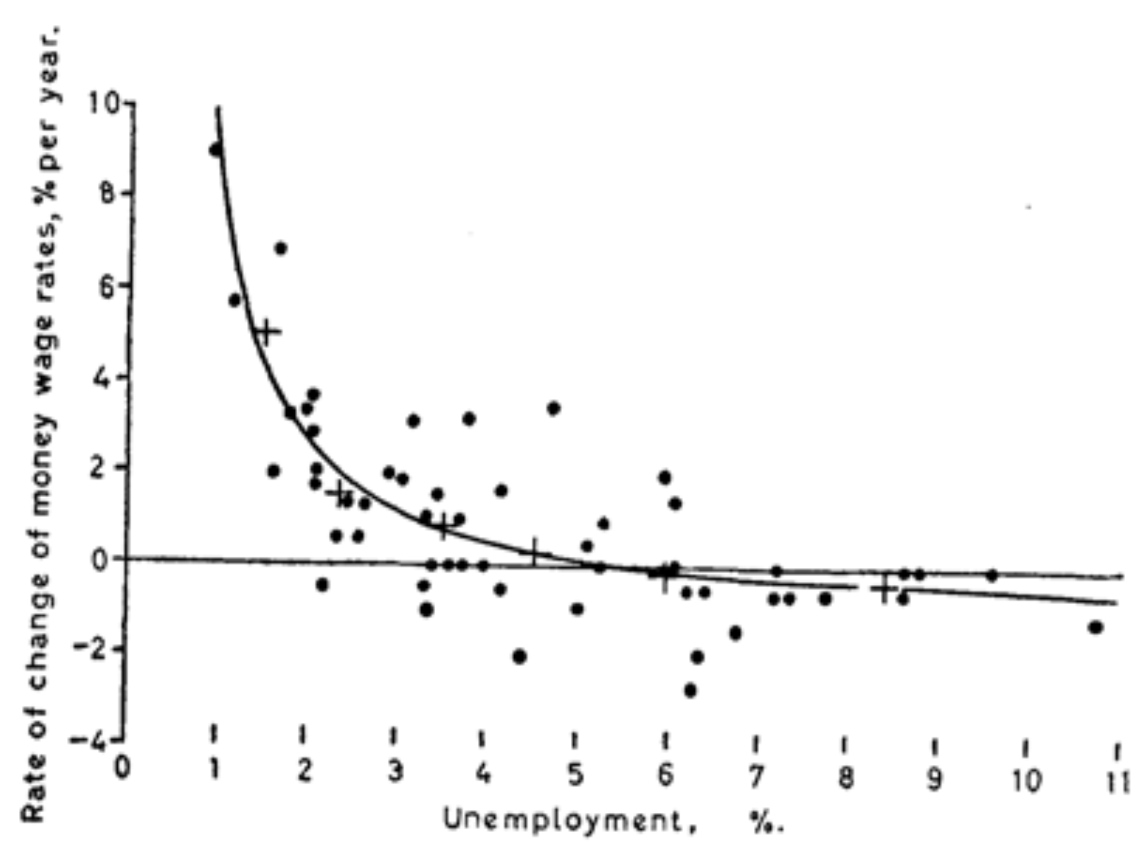
3.1. The “Original” Phillips Curve

Phillips in [3] used British econometric data–the rate of change of money wage rates, provided by the Board of Trade and the Ministry of Labour (calculated by Phelps Brown and Sheila Hopkins [55]), and corresponding percentage employment data, quoted in [56]. But, for a simpler evaluation, the data were first preprocessed, i.e., the average values of the rate of change of money wage rates and of the percentage unemployment for six different levels of the unemployment (0–2, 2–3, 3–4, 4–5, 5–7, 7–11) were calculated. The crosses in the Figure 1 refer to these average values. Phillips then fitted a curve to the crosses using a model in the form:

$$\begin{array}{cc}\hfill y+a& =b{x}^c\Rightarrow \hfill \\ \hfill log(y+a)& =logb+clogx,\hfill \end{array}$$

(3)

where y stands for the rate of change of wage rates and x for the percentage unemployment. The parameters b and c were estimated using the least squares to fit four crosses laying between 0–5% of unemployment, and the parameter a was chosen to fit the remaining two crosses laying in the interval 5–11% of unemployment. Based on this “fitting criterion” Phillips identified the parameters of the model (3) as follows:

$$\begin{array}{cc}\hfill y+0.900& =9.638x^{-1.394}\Rightarrow \hfill \\ \hfill log(y+0.900)& =0.984-1.394logx.\hfill \end{array}$$

Figure 1. “Original” Phillips curve [3] (with permission from the John Wiley and Sons publisher).

3.2. The Mittag-Leffler Model for Fitting the Phillips Curve

The idea to use an ML-type function to describe the econometric data (representing the Phillips curve) results naturally from the observation of two facts:

• the simplicity of the model used by Phillips in his paper [3] given in (3), where a power-type regression is used to fit the data, and where the model can be defined in the form:

  $$\begin{array}{c}\hfill y\left(x\right)=b{x}^c-a,a,b,c\in \mathbb{R},\end{array}$$

  (4)
• the usual shape of the PC, used in the literature, which reminds on the exponential-type function:

  $$\begin{array}{c}\hfill y\left(x\right)=b{e}^{cx}-a,a,b,c\in \mathbb{R},\end{array}$$

  (5)

where for both cases, (4) and (5), x stands for the unemployment rate and y for the inflation rate.

Based on these facts, the one-parameter ML function appears to be a general model to fit the PC relation, as it behaves between a purely exponential function and a power function. The one-parameter ML function defined in (1), which includes the special case when $\alpha =1$, i.e., the classical exponential function, is used to model the econometric data under study. Generally, the proposed fitting model can be written as follows:

$$\begin{array}{c}\hfill y\left(x\right)=c{E}_{\alpha }\left(b{x}^{\alpha }\right),\alpha \in \mathbb{C},Re\left(\alpha \right)>0,b,c\in \mathbb{R},\end{array}$$

(6)

where the parameters $\alpha ,b,c$ are subject to optimisation procedure minimising the squared sum of the vertical offsets between the data points and the fitting curve. Some of the possible manifestations of the ML model given in (6) are shown in Figure 2 (figures generated using the Matlab demo published by Igor Podlubny [57]), with the identified parameters listed in Table 1.

Figure 2. Mittag-Leffler fitting using different functions y(x) for generating data [57].

Table 1. Identified parameters of the Mittag-Leffler fitting model: $y\left(x\right)=c{E}_{\alpha }\left(b{x}^{\alpha }\right)$.

		$\mathit{y}\left(\mathit{x}\right)={\mathit{e}}^{\mathit{x}}erfc\left(\sqrt{\mathit{x}}\right)$	$\mathit{y}\left(\mathit{x}\right)=\mathit{c}{\mathit{E}}_{\mathit{\alpha }}\left(\mathit{b}{\mathit{x}}^{\mathit{\alpha }}\right)$	$\mathit{y}\left(\mathit{x}\right)=cos\left(\mathit{x}\right)$	$\mathit{y}\left(\mathit{x}\right)={\mathit{e}}^{-\mathit{d}\mathit{x}}cos\left(\mathit{x}\right)$
	c	-	0.8	-	-
generating	$\alpha$	-	1.5	-	-
parameters	b	-	−0.2	-	-
	d	-	-	-	0.2
	c	0.9982	0.7869	1.0045	0.9722
identified	$\alpha$	0.5008	1.4999	2.0000	1.7538
parameters	b	−0.9974	−0.1988	−0.9999	−1.0327

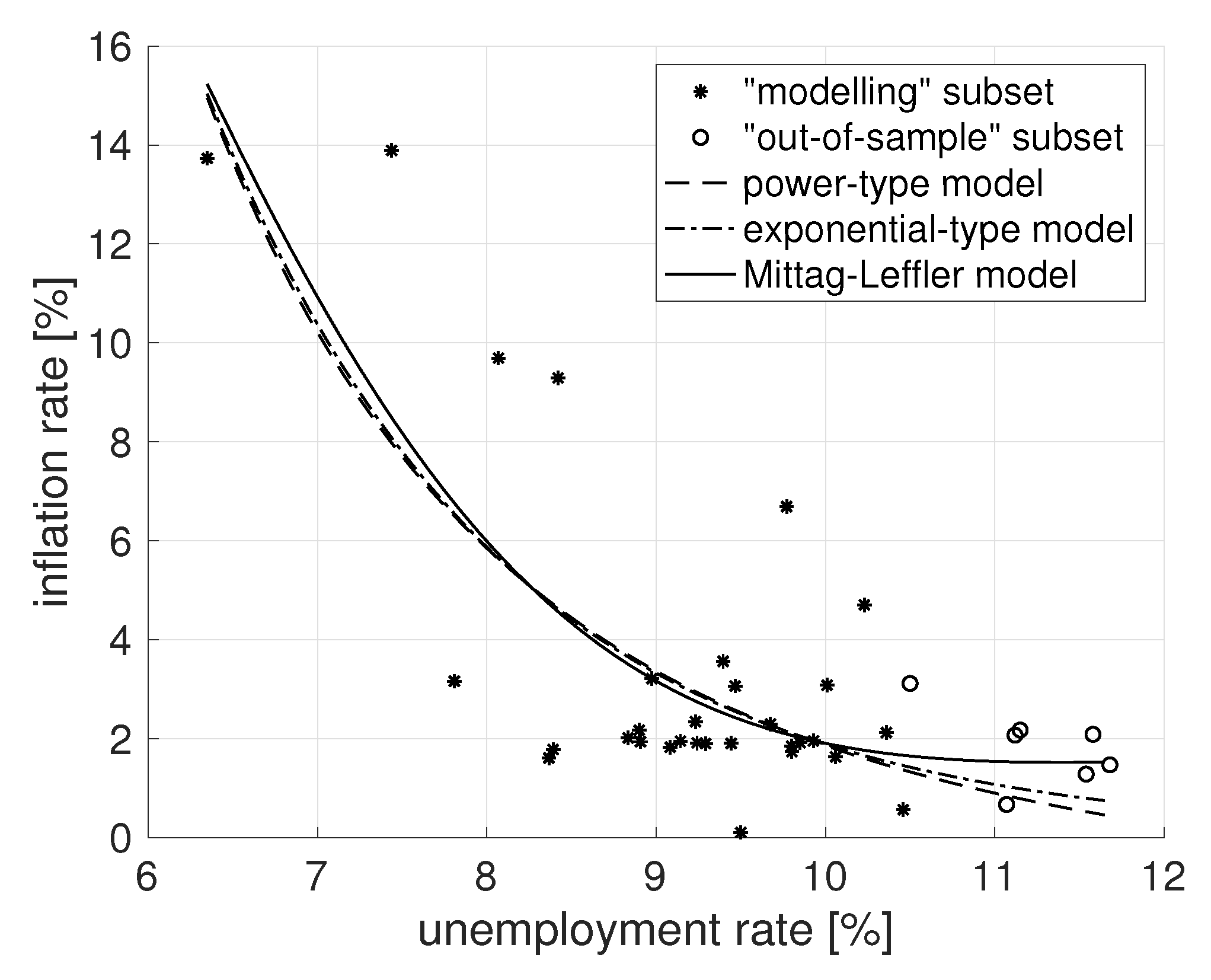
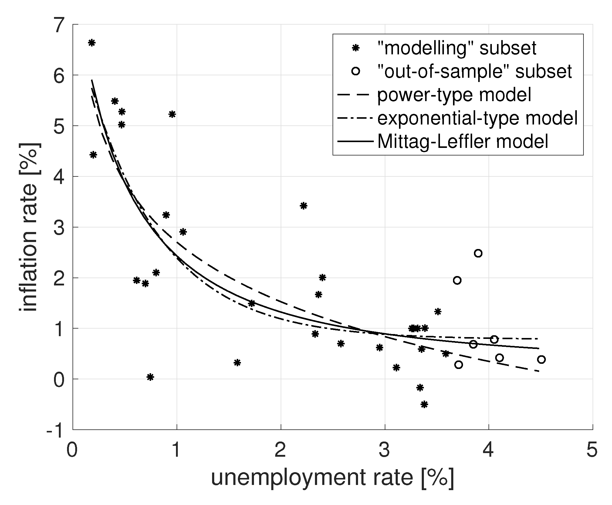
4. Numerical Results and Discussion

To evaluate the performance of the proposed ML model (6) in comparison to the power-type model (4), and the exponential-type model (5) the econometric data of two European countries (France and Switzerland) were used, that were obtained from the EconStats^TM portal [43]. The unemployment rate and the inflation rate were taken for the period of time 1980–2017. The whole list of the processed data can be found in the Table A1.

4.1. Goodness-of-Fit Statistics and Data Preprocessing

The sum of squared errors (SSE) between the fitting models and the used data serves as the fitting-criterion, with values closer to 0 indicating a smaller random error component of the model. Also some other quality measures were evaluated, i.e., the R-square from interval $[0,1]$, that indicates the proportion of variance satisfactory explained by the fitting-model (e.g., R-square $=0.7325$ means that the fit explains $73.25\%$ of the total variation in the data about the average); the adjusted R-square statistic, with values smaller or equal to 1, where values closer to 1 indicate a better fit; the root mean squared error (RMSE), with values closer to 0 indicating a fit more useful for prediction [58].

The used dataset, where the unemployment rate corresponds to the x-coordinate and the inflation rate corresponds to the y-coordinate (each sample represents the state of these two indicators for each year from the period under study), is first split into two subsets, the “modelling” subset is used to identify the model parameters, the “out-of-sample” subset serves for evaluating the forecast-performance of the models. For both economies, French and Swiss, all three models were first fitted to the data from the “modelling” subset (composed of 31 samples), by minimising SSE, identifying the optimal parameters. The obtained parameters were then used to compute SSE of the identified models to the “out-of-sample” subset (composed of seven samples with the greatest values of unemployment rate) and SSE of the fitting model to the complete dataset.

4.2. Experiments

The first experiment was conducted using the French econometric data. The modelling subset of 31 samples, was used for the identification purposes. All three models, the power-type model (4), the exponential-type model (5), and the ML model (6), were fitted to these data minimising the SSE obtaining so the optimal parameters. The identified models were then used to compute the SSE to the complete dataset of 38 samples (including the “out-of-sample” subset). SSE results to the modelling subset as well as SSE to the “out-of-sample” subset and SSE to the complete dataset for the French Phillips curve are shown in Table 2, alongside the values of R-square, adjusted R-square, and RMSE. The ML model outperformed the compared models in all listed statistic indicators, with SSE to the “out-of-sample” subset double smaller than the exponential-type model, and almost three-times smaller than the power-type model (see Table 2, where bold stands for better result).

Table 2. The statistical results of the French Phillips curve fitting.

	Power-Type Model	Exponential-Type Model	ML Model
SSE to “modelling’’ subset	157.8422	155.8276	149.6035
SSE to “out-of-sample’’ subset	10.9024	8.0347	3.9904
SSE to complete dataset	168.7446	163.8623	153.5939
R-square	0.5634	0.5690	0.5862
adjusted R-square	0.5322	0.5382	0.5567
RMSE	2.3740	2.3590	2.3110
Model	$y\left(x\right)=b{x}^c-a$	$y\left(x\right)=b{e}^{cx}-a$	$y\left(x\right)=c{E}_{\alpha }\left(b{x}^{\alpha }\right)$
definition
	$a=1.552$	$a=-0.0187$	$\alpha =1.358$
Identified	$b=1.009e+04$	$b=563.6$	$b=-0.6378$
parameters	$c=-3.471$	$c=-0.571$	$c=-149.9$

The result of the French Phillips curve fitting is also shown in Figure 3, where it is possible to observe a similar behaviour of all three models, i.e., with the increase of the unemployment rate the inflation rate exponentially decreases. However, for the last samples, the decrease of the ML model slows down in comparison to the power-type and exponential-type models. This behaviour of the ML model is obviously better describing the trend of the “out-of-sample” subset. This is also confirmed by the smallest SSE value of the ML fitting curve to the “out-of-sample” subset (see Table 2).

Figure 3. Fitting the French Phillips curve.

Identically as in the French case, the Swiss econometric data (unemployment rate and inflation rate) were first preprocessed. The complete dataset was split into the “modelling” subset composed of 31 samples, that was used to identify the optimal parameters of the power-type model (4), the exponential-type model (5), and the ML model (6). The SSE between the “modelling” subset and the fitting curves was again used as the fitting criterion. Using the identified model parameters the SSE of the evaluated models to the complete dataset of 38 samples (including the “out-of-sample” subset) was computed. In order to compare the forecast-performance of the models SSE to the “out-of-sample” subset, as well as the SSE values for the “modelling” subset fitting, and SSE to the complete dataset for the Swiss Phillips Curve are shown in Table 3, alongside the values of R-square, adjusted R-square, and RMSE.

Table 3. The statistical results of the Swiss Phillips curve fitting.

	Power-Type Model	Exponential-Type Model	ML Model
SSE to “modelling’’ subset	39.6506	40.0588	39.2992
SSE to “out-of-sample’’ subset	6.8961	4.6826	5.0041
SSE to complete dataset	46.5466	44.7414	44.3033
R-square	0.6389	0.6351	0.6420
adjusted R-square	0.6131	0.6091	0.6165
RMSE	1.1900	1.1960	1.1850
Model	$y\left(x\right)=b{x}^c-a$	$y\left(x\right)=b{e}^{cx}-a$	$y\left(x\right)=c{E}_{\alpha }\left(b{x}^{\alpha }\right)$
definition
	$a=-551.3$	$a=-0.7809$	$\alpha =0.7733$
Identified	$b=-548.6$	$b=6.364$	$b=-1.468$
parameters	$c=30.85e-04$	$c=-1.376$	$c=8.823$

Observing the result of the Swiss Phillips curve fitting shown in Figure 4, one can see an interesting case, where although all the compared models are exponentially decreasing, the curve representing the proposed ML model proceeds in-between the power-type and the exponential-type models, that form a kind of scissors. In respect to the “out-of-sample” subset it is possible to conclude that two points of that subset deviate, having higher inflation rate value then the others. This strongly influenced the fitting results. In this case the exponential-type model visually represents the “out-of-sample” subset slightly better then the ML model, that is also demonstrated by a smaller value of SSE of the exponential-type model to the “out-of-sample” subset (see Table 3). In spite of this, the ML model outperforms the compared models in all other used statistic indicators, including smaller SSE to the complete dataset, proving it’s capability. Moreover, in case of filtering these two outliers from the “out-of-sample” subset, the ML model better fits the data-trend.

Figure 4. Fitting the Swiss Phillips curve.

5. Conclusions

The ability of the Mittag-Leffler function to behave between the power-type and the exponential-type function, and moreover to fit data that manifest signs of stretched exponentials, oscillations or damped oscillations is demonstrated in this paper, with application to fitting the econometric data (Phillips curve) of two European economies, where the proposed ML model outperforms the compared fitting-models in terms of the chosen performance criterions. Exploiting the full potential of the Mittag-Leffler function and it’s generalisations, as well as associating the model parameters with the corresponding economic indicators will be the topic of further work.

References

- Samuelson, P.A.; Solow, R.M. Analytical aspects of anti-inflation policy. Am. Econ. Rev. 1960, 50, 177–194. [Google Scholar]
- Fisher, I. A Statistical Relation between Unemployment and Price Changes. Int. Labour Rev. 1926, 13, 785–792. [Google Scholar]
- Phillips, A.W. The relation between unemployment and the rate of change of money wage rates in the United Kingdom, 1861–1957. Economica 1958, 25, 283–299. [Google Scholar] [CrossRef]
- Brown, A.J. Great Inflation 1939–1951; Oxford University Press: London, UK, 1955. [Google Scholar]
- Lipsey, R.G. The relation between unemployment and the rate of change of money wage rates in the United Kingdom, 1862–1957: A further analysis. Economica 1960, 27, 1–31. [Google Scholar] [CrossRef]
- Bowen, W.G. Wage Behavior in the Postwar Period: An Empirical Analysis; Princeton University: Princeton, NJ, USA, 1960. [Google Scholar]
- Bodkin, R.G. The Wage-Price-Productivity Nexus; University of Pennsylvania Press: Philadelphia, PA, USA, 1966. [Google Scholar]
- Taylor, J.B. Aggregate dynamics and staggered contracts. J. Polit. Econ. 1980, 88, 1–23. [Google Scholar] [CrossRef]
- Calvo, G.A. Staggered Prices In A Utility-maximizing Framework. J. Monetary Econ. 1983, 12, 383–398. [Google Scholar] [CrossRef]
- Rotemberg, J.J.; Woodford, M. An Optimization-Based Econometric Framework for the Evaluation of Monetary Policy. In NBER Macroeconomics Annual; MIT Press: Cambridge, MA, USA, 1997; pp. 297–346. [Google Scholar]
- Friedman, M. The role of monetary policy. Am. Econ. Rev. 1968, 58, 1–17. [Google Scholar]
- Phelps, E.S. Money-Wage Dynamics and Labor Market Equilibrium. J. Polit. Econ. 1968, 76, 678–711. [Google Scholar] [CrossRef]
- Clarida, R.; Galí, J.; Gertler, M. The science of monetary policy: A new Keynesian perspective. J. Econ. Lit. 1999, 37, 1661–1707. [Google Scholar] [CrossRef]
- Galí, J.; Gertler, M.; López-Salido, J.D. Robustness of the Estimates of the Hybrid New Keynesian Phillips Curve. J. Monetary Econ. 2005, 52, 1107–1118. [Google Scholar] [CrossRef]
- Mittag-Leffler, M.G. Une generalisation de l’integrale de Laplace-Abel. Comptes Rendus de l’Académie des Sciences 1903, 137, 537–539. [Google Scholar]
- Mittag-Leffler, M.G. Sur la nouvelle fonction Eα(x). Comptes Rendus de l’Académie des Sciences 1903, 137, 554–558. [Google Scholar]
- Dzhrbashyan, M.M. Integral Transforms and Representations of Functions in Complex Plane; Nauka: Moscow, Russia, 1966. [Google Scholar]
- Caputo, M.; Mainardi, F. Linear models of dissipation in anelastic solids. La Rivista del Nuovo Cimento 1971, 1, 161–198. [Google Scholar] [CrossRef]
- Blair, G.W.S. Psychorheology: links between the past and the present. J. Texture Stud. 1974, 5, 3–12. [Google Scholar] [CrossRef]
- Torvik, P.J.; Bagley, R.L. On the appearance of the fractional derivative in the behaviour of real materials. J. Appl. Mech. 1984, 51, 294–298. [Google Scholar] [CrossRef]
- Samko, S.G.; Kilbas, A.A.; Marichev, O.I. Fractional Integrals and Derivatives: Theory and Applications; Gordon and Breach: New York, NY, USA, 1993. [Google Scholar]
- Gorenflo, R.; Kilbas, A.A.; Mainardi, F.; Rogosin, S.V. Mittag-Leffler Functions, Related Topics and Applications; Springer Monographs in Mathematics; Springer: Berlin/Heidelberg, Germany, 2014. [Google Scholar] [CrossRef]
- Kilbas, A.A.; Saigo, M.; Saxena, R.K. Generalized Mittag-Leffler function and generalized fractional calculus operators. Integral Transform. Spec. Funct. 2004, 15, 31–49. [Google Scholar] [CrossRef]
- Mainardi, F.; Gorenflo, R. On Mittag-Leffler-type functions in fractional evolution processes. J. Comput. Appl. Math. 2000, 118, 283–299. [Google Scholar] [CrossRef]
- West, B.; Mauro Bologna, M.; Grigolini, P. Physics of Fractal Operators; Springer: New York, NY, USA, 2003. [Google Scholar]
- Haubold, H.J.; Mathai, A.M.; Saxena, R.K. Mittag-Leffler functions and their applications. J. Appl. Math. 2011, 2011, 51. [Google Scholar] [CrossRef]
- Chen, Y. Generalized Generalized Mittag-Leffler function. MathWorks, Inc. Matlab Central File Exchange. 2008. Available online: http://www.mathworks.com/matlabcentral/fileexchange/21454 (accessed on 21 May 2019).
- Podlubny, I. Mittag-Leffler Function. MathWorks, Inc. Matlab Central File Exchange. 2005. Available online: http://www.mathworks.com/matlabcentral/fileexchange/8738 (accessed on 21 May 2019).
- Garrappa, R. The Mittag-Leffler function. MathWorks, Inc. Matlab Central File Exchange. 2015. Available online: http://www.mathworks.com/matlabcentral/fileexchange/48154 (accessed on 21 May 2019).
- Capelas de Oliveira, E.; Mainardi, F.; Vaz, J., Jr. Models based on Mittag-Leffler functions for anomalous relaxation in dielectrics. Eur. Phys. J. Spec. Top. 2011, 193, 161–171. [Google Scholar] [CrossRef]
- Petras, I.; Sierociuk, D.; Podlubny, I. Identification of Parameters of a Half-Order System. IEEE Trans. Signal Process. 2012, 60, 5561–5566. [Google Scholar] [CrossRef]
- Maindardi, F. Fractional Calculus and Waves in Linear Vescoelasticity: An Introduction to Mathematical Models (Second Revised Edition); Imperial College Press: London, UK, 2018. [Google Scholar]
- Samuel, S.; Ricon, J.; Podlubny, I. Modelling combustion in internal combustion engines using the Mittag-Leffler function. In Proceedings of the ICFDA 16: International Conference on Fractional Differentiation and its Applications, Novi Sad, Serbia, 18–20 July 2016; pp. 551–552. [Google Scholar]
- Zeng, C.; Chen, Y.; Podlubny, I. Is our universe accelerating dynamics fractional order? In Proceedings of the 2015 ASME/IEEE International Conference on Mechatronic and Embedded Systems and Applications, Boston, MA, USA, 2–5 August 2015. Paper No. DETC2015-46216. [Google Scholar]
- Atangana, A.; Baleanu, D. New Fractional Derivatives With Non-Local And Non-Singular Kernel: Theory and Application to Heat Transfer Model. Therm. Sci. 2016, 20-2, 763–769. [Google Scholar] [CrossRef]
- Scalas, E.; Gorenflo, R.; Mainardi, F. Fractional calculus and continuous-time finance. Phys. A Stat. Mech. Its Appl. 2000, 284, 376–384. [Google Scholar] [CrossRef]
- Cartea, A.; del Castillo-Negrete, D. Fractional diffusion models of option prices in markets with jumps. Phys. A Stat. Mech. Its Appl. 2007, 374, 749–763. [Google Scholar] [CrossRef]
- Garibaldi, U.; Scalas, E. Finitary Probabilistic Methods in Econophysics; Cambridge University Press: Cambridge, UK, 2010. [Google Scholar]
- Skovranek, T.; Podlubny, I.; Petras, I. Modeling of the national economies in state-space: A fractional calculus approach. Econ. Model. 2012, 29, 1322–1327. [Google Scholar] [CrossRef]
- Tarasov, V.E.; Tarasova, V.V. Macroeconomic models with long dynamic memory: Fractional calculus approach. Appl. Math. Comput. 2018, 338, 466–486. [Google Scholar] [CrossRef]
- Tarasov, V.E.; Tarasova, V.V. Phillips model with exponentially distributed lag and power-law memory. Comput. Appl. Math. 2019, 38, 13. [Google Scholar] [CrossRef]
- Tarasov, V.E.; Tarasova, V.V. Dynamic Keynesian Model of Economic Growth with Memory and Lag. Mathematics 2019, 7, 178. [Google Scholar] [CrossRef]
- Econstats.com. EconStats: World Economic Outlook (WEO) data, IMF. 2019. Available online: http://www.econstats.com (accessed on 21 May 2019).
- Erdélyi, A.; Magnus, W.; Oberhettinger, F.; Tricomi, F.G. Higher Transcendental Functions; McGraw-Hill: New York, NY, USA, 1955; Volume 3. [Google Scholar]
- Mittag-Leffler, M.G. Sopra la funzione Eα(x). Comptes Rendus de l’Académie des Sciences 1904, 13, 3–5. [Google Scholar]
- Wiman, A. Über den Fundamentalsatz in der Teorie der Funktionen Eα(x). Acta Math. 1905, 29, 191–201. [Google Scholar] [CrossRef]
- Pollard, H. The completely monotonic character of the Mittag-Leffler function Ea(−x). Bull. Am. Math. Soc. 1948, 54, 1115–1116. [Google Scholar] [CrossRef]
- Humbert, P.; Agarwal, R.P. Sur la fonction de Mittag-Leffler et quelques-unes de ses généralisations. Bulletin des Sciences Mathématiques 1953, 77, 180–185. [Google Scholar]
- Cover, J.P. Asymmetric effects of positive and negative money-supply shocks. Q. J. Econ. 1992, 107, 1261–1282. [Google Scholar] [CrossRef]
- Karras, G. Are the output effects of monetary policy asymmetric? Evidence from a sample of European countries. Oxf. Bull. Econ. Stat. 1996, 58, 267–278. [Google Scholar] [CrossRef]
- Nobay, A.R.; Peel, D.A. Optimal monetary policy with a nonlinear Phillips curve. Econ. Lett. 2000, 67, 159–164. [Google Scholar] [CrossRef]
- Schaling, E. The nonlinear Phillips curve and inflation forecast targeting: Symmetric versus asymmetric monetary policy rules. J. Money Credit Bank. 2004, 36, 361–386. [Google Scholar] [CrossRef][Green Version]
- Stiglitz, J. Reflections on the natural rate hypothesis. J. Econ. Perspect. 1997, 11, 3–10. [Google Scholar] [CrossRef]
- Filardo, A. New evidence on the output cost of fighting inflation. Fed. Reserve Bank Kansas City Econ. Rev. 1998, 83, 33–61. [Google Scholar]
- Brown, P.; Hopkins, S. The Course of Wage-Rates in Five Countries, 1860–1939. Oxf. Econ. Pap. 1950, 2, 226–296. [Google Scholar] [CrossRef]
- Beveridge, H.W. Full Employment in a Free Society; W. W. Norton & Co., Inc.: New York, NY, USA, 1945. [Google Scholar]
- Podlubny, I. Fitting Data Using the Mittag-Leffler Function. MathWorks, Inc. Matlab Central File Exchange. 2011. Available online: http://www.mathworks.com/matlabcentral/fileexchange/32170 (accessed on 21 May 2019).
- MathWorks, Inc. Evaluating Goodness of Fit. 2019. Available online: https://www.mathworks.com/help/curvefit/evaluating-goodness-of-fit.html (accessed on 21 May 2019).
© 2019 by the author. Licensee MDPI, Basel, Switzerland. This article is an open access article distributed under the terms and conditions of the Creative Commons Attribution (CC BY) license (http://creativecommons.org/licenses/by/4.0/).