On a Bi-Parametric Family of Fourth Order Composite Newton–Jarratt Methods for Nonlinear Systems

Abstract

We present a new two-parameter family of fourth-order iterative methods for solving systems of nonlinear equations. The scheme is composed of two Newton–Jarratt steps and requires the evaluation of one function and two first derivatives in each iteration. Convergence including the order of convergence, the radius of convergence, and error bounds is presented. Theoretical results are verified through numerical experimentation. Stability of the proposed class is analyzed and presented by means of using new dynamics tool, namely, the convergence plane. Performance is exhibited by implementing the methods on nonlinear systems of equations, including those resulting from the discretization of the boundary value problem. In addition, numerical comparisons are made with the existing techniques of the same order. Results show the better performance of the proposed techniques than the existing ones.

1. Introduction

The construction of fixed-point methods for nonlinear equations is an interesting and important task in numerical analysis and many applied scientific disciplines. This has led to the development of many numerical methods, frequently of an iterative nature. In the past few decades, the iterative techniques have been applied in many diverse fields such as economics, engineering, physics, dynamical models, and so on.

In this paper, we consider the problem of finding the solution of nonlinear equations $F\left(x\right)=0$ ($F:\Omega \subseteq B\to B$, B is a Banach space and $\Omega$ a non-empty convex open set) by iterative methods of convergence order four. The solution vector (say, $x^{*}$) can be computed as a fixed point of some function $M:\Omega \subseteq B\to B$ by using fixed-point iteration

$$\begin{array}{c}{\displaystyle x_0\in \Omega ,}\hfill \\ {\displaystyle x_{n+1}=M\left(x_n\right),n\ge 0.}\hfill \end{array}$$

(1)

Newton’s method [1,2,3] is the most widely used technique for solving nonlinear equations. This method has quadratic convergence under the conditions that the function F is continuously differentiable and a close initial estimate $x_0$ is given. We define this method as

$$x_{n+1}=x_n-F^{\prime }{\left(x_n\right)}^{-1}F\left(x_n\right),$$

(2)

where $F^{\prime }{\left(x\right)}^{-1}$ is the inverse of the Frèchet-derivative $F^{\prime }\left(x\right)$.

Based on Newton’s or Newton-like iterations, many higher order methods have been proposed in the literature. For example, Cordero-Torregrosa [4], Frontini-Sormani [5], Grau et al. [6], Homeier [7] and Noor-Waseem [8] have proposed third-order methods where each requires three evaluations per iteration namely, one F and two $F^{\prime }$. Cordero-Torregrosa also introduced two third-order methods in [4], one method requires the evaluations of one F and three $F^{\prime }$, while the other requires one F and four $F^{\prime }$. Darvishi-Barati [9] have derived a third-order method that utilizes two F and one $F^{\prime }$. Babajee et al. [10] have presented a fourth order method requiring one F and two $F^{\prime }$. In [11], Cordero et al. implemented fourth order Jarratt’s method [12] for scalar equations to systems of equations, that uses one F and two $F^{\prime }$. Cordero et al. also presented a fourth order method requiring two F and two $F^{\prime }$ in [13]. Darvishi-Barati developed a fourth order method in [14] which requires two F and three $F^{\prime }$. Grau et al. developed a fourth order method in [6] that uses three F and one $F^{\prime }$ per iteration. Grau et al. [15] also generalized the fourth order Ostrowski-like [16] and Ostrowski’s [3] methods to systems of nonlinear equations each of which utilizes two F, one $F^{\prime }$ and one divided difference per iteration. In [17], Hueso et al. presented a fourth order method which requires one F and two $F^{\prime }$. Noor and Noor in [18] developed a fourth order method that uses three F and one $F^{\prime }$. Sharma and Arora proposed a fourth order method in [19] requiring one F and two $F^{\prime }$ in each iteration. Apart from these third and fourth-order methods, researchers have also proposed some higher order methods, see, for example [11,13,15,17,20,21,22,23,24] and references therein.

One of the important problems related to iterative methods is to study their complex dynamics. This study allows us to find the best members of a family of iterative methods in terms of stability, and once we have found those members, we can know the points that converge to any of the roots. That is the reason why the study of dynamical behavior of a family of iterative methods is so important. Learning of the complex dynamics of iterative methods has an historic importance since Schröder in 1870 and later Cayley in 1879 proposed to study Newton’s method in order to find the solutions of an equation in the complex plane. One of the most famous problems in this area is known as “the Cayley’s” problem, in which Cayley tried to characterize the basins of attraction of each of the roots of a cubic polynomial using Newton’s method. Firstly, he characterized the basins of attraction of a quadratic polynomial, that was easy as the Julia set was the mediatrix of the segment joining both roots. In the cubic case, he was not able to find that characterization. Nowadays, with the use of computers, and symbolic and numerical software we can draw those basins and we can understand how difficult it is to draw them without computers. In recent times, many authors have analyzed the complex dynamics of iteration functions in their work, see [17,25,26,27,28] and references therein.

In this paper, we present a two-parameter family of iterative methods with fourth order convergence. The scheme is composed of two steps and requires the evaluations of one function and two first order derivatives in each iteration. For a set of parametric values, the Jarratt’s method [11] is a special case of the family. In order to make the paper self-contained, we provide local convergence including convergence radius, error bounds, and estimates on the uniqueness of the solution. Moreover, the stability of the methods is analyzed and presented by means of using dynamic tools, namely, convergence plane and basins of attraction. The efficiency is demonstrated by implementing the methods on some different systems of nonlinear equations.

We summarize the contents of the paper. Section 2 contains the development of the family of methods along with fourth order of convergence. The local convergence of methods is presented in Section 3. The dynamical behavior of the family is analyzed in Section 4. In Section 5, numerical examples are considered to verify the theoretical results. In Section 6 the methods are applied to solve systems of nonlinear equations of different nature. Concluding remarks are given in Section 7.

2. Development of Method

Let us consider the scheme

$$\begin{array}{cc}\hfill z_n=& x_n-\frac{2}{3}{F}^{\prime }{\left(x_n\right)}^{-1}F\left(x_n\right),\hfill \\ x_{n+1}=\hfill & x_n-F^{\prime }{\left(x_n\right)}^{-1}F\left(x_n\right)+F^{\prime }{\left(x_n\right)}^{-1}{D}_n{C}_n^{-1}F\left(x_n\right),\hfill \end{array}$$

(3)

where $C_n=r{F}^{\prime }\left(x_n\right)+t{F}^{\prime }\left(z_n\right),$$D_n=C_n-\frac{1}{2}{F}^{\prime }\left(x_n\right)A_n^{-1}{B}_n$, $A_n=3(3r+t)F^{\prime }\left(z_n\right)-(3r+5t)F^{\prime }\left(x_n\right)$, $B_n=(9r^2+30rt+5t^2)F^{\prime }\left(z_n\right)+(3r^2-22rt-9t^2)F^{\prime }\left(x_n\right)$, and r and t are arbitrary constants. This is a scheme which uses Jarratt’s step as the first step whereas Newton–Jarratt composition in the second step (see, [11]). For this reason, we shall call it the composite Newton–Jarratt scheme.

We introduce some known notations and results [11], which are needed to obtain the convergence order of new method. Let $F:\Omega \subseteq {\mathbb{R}}^m\to {\mathbb{R}}^m$ be sufficiently differentiable in $\Omega$. The qth derivative of F at $u\in {\mathbb{R}}^m$, $q\ge 1$, is the q-linear function $F^{\left(q\right)}\left(u\right):{\mathbb{R}}^m\times \cdots \times {\mathbb{R}}^m\to {\mathbb{R}}^m$ such that $F^{\left(q\right)}\left(u\right)(v_1,\dots ,v_q)\in {\mathbb{R}}^m$. It can be easily seen that

(i)

$F^{\left(q\right)}\left(u\right)(v_1,\dots ,v_{q-1},\dots )\in \mathcal{L}\left({\mathbb{R}}^m\right)$,

(ii)

$F^{\left(q\right)}\left(u\right)(v_{\sigma \left(1\right)},\dots ,v_{\sigma \left(q\right)})=F^{\left(q\right)}\left(u\right)(v_1,\dots ,v_q)$, ∀ permutation $\sigma$ of $\{1,2,\dots ,q\}$.

From the above expressions, we can use the following notation:

(a)

$F^{\left(q\right)}\left(u\right)(v_1,\dots ,v_q)=F^{\left(q\right)}\left(u\right)v_1,\dots ,v_q$,

(b)

$F^{\left(q\right)}\left(u\right)v^{q-1}{F}^{\left(p\right)}\left(u\right)v^p=F^{\left(q\right)}\left(u\right)F^{\left(p\right)}\left(u\right)v^{q+p-1}$.

On the other hand, assuming that the Jacobian matrix $F^{\prime }\left(x^{*}\right)$ is nonsingular we can apply Taylor’s expansion for $x^{*}+h\in {\mathbb{R}}^m$ lying in a neighborhood of a solution $x^{*}$ of $F\left(x\right)=0$, that is

$$F(x^{*}+h)=F^{\prime }\left(x^{*}\right)\left[h+\sum _{q=2}^{p-1}{K}_q{h}^q\right]+O\left(h^p\right),$$

(4)

where $K_q=\frac{1}{q!}{F}^{\prime }{\left(x^{*}\right)}^{-1}{F}^{\left(q\right)}\left(x^{*}\right)$, $q\ge 2$. Notice that $K_q{h}^q\in {\mathbb{R}}^m$ since $F^{\left(q\right)}\left(x^{*}\right)\in \mathcal{L}({\mathbb{R}}^m\times \cdots \times {\mathbb{R}}^m,{\mathbb{R}}^m)$ and $F^{\prime }{\left(x^{*}\right)}^{-1}\in \mathcal{L}\left({\mathbb{R}}^m\right)$. Also, we have that

$$F^{\prime }(x^{*}+h)=F^{\prime }\left(x^{*}\right)\left[I+\sum _{q=2}^{p-1}q{K}_q{h}^{q-1}\right]+O\left(h^{p-1}\right),$$

(5)

where I is the identity matrix. Therefore, $q{K}_q{h}^{q-1}\in \mathcal{L}\left({\mathbb{R}}^m\right)$. From (5), we obtain

$$F^{\prime }{(x^{*}+h)}^{-1}=\left[I+X_{2}h+X_3{h}^2+X_4{h}^3+\cdots \right]F^{\prime }{\left(x^{*}\right)}^{-1}+O\left(h^p\right),$$

(6)

where

$$\begin{array}{cc}{X}_2=\hfill & -2K_2,\hfill \\ X_3=\hfill & 4K_2^2-3K_3,\hfill \\ X_4=\hfill & -8K_2^3+6K_2{K}_3+6K_3{K}_2-4K_4,\hfill \\ & ⋮\hfill \end{array}$$

(7)

Let $e_n=x_n-x^{*}$ be the error in the nth iteration, then the equation

$$e_{n+1}=M{\left(e_n\right)}^p+O\left({\left(e_n\right)}^{p+1}\right),$$

(8)

where M is a p-linear function $M\in \mathcal{L}({\mathbb{R}}^m\times \cdots \times {\mathbb{R}}^m,{\mathbb{R}}^m)$, is called the error equation and p is the order of convergence. Note that ${\left(e_n\right)}^p$ is $(e_n,e_n,\stackrel{p}{\dots },e_n)$.

We show that the scheme (3) has the fourth order of convergence with the help of following theorem:

Theorem 1.

Let $F:\Omega \subseteq {\mathbb{R}}^m\to {\mathbb{R}}^m$ be a sufficiently many times differentiable mapping. Moreover, suppose that there exists a solution $x^{*}$ of $F\left(x\right)=0$ such that $F^{\prime }{\left(x^{*}\right)}^{-1}$ is invertible. Then, sequence $\left\{x_n\right\}$ generated by method (3) for $x_0\in \Omega$ converges to $x^{*}$ with convergence order four provided that $3r-t\ne 0$ and $r+t\ne 0$.

Proof. 

Let $e_n=x_n-x^{*}$ for $n=0,1,2\dots$ and $\Gamma =F^{\prime }{\left(x_n\right)}^{-1}$. Then the Taylor’s expansion of $F\left(x_n\right)$ in a neighborhood of $x^{*}$ yields

$$F\left(x_n\right)=F^{\prime }\left(x^{*}\right)(e_n+K_2{\left(e_n\right)}^2+K_3{\left(e_n\right)}^3+K_4{\left(e_n\right)}^4+O\left({\left(e_n\right)}^5\right)).$$

(9)

Also,

$$F^{\prime }\left(x_n\right)=F^{\prime }\left(x^{*}\right)(I+2K_2{e}_n+3K_3{\left(e_n\right)}^2+4K_4{\left(e_n\right)}^3+O\left({\left(e_n\right)}^4\right)).$$

(10)

Inversion of $F^{\prime }\left(x_n\right)$ yields,

$$\begin{array}{cc}{F}^{\prime }{\left(x_n\right)}^{-1}=(I\hfill & -2K_2{e}_n+(4K_2^2-3K_3){\left(e_n\right)}^2-(4K_4-6K_2{K}_3-6K_3{K}_2+8K_2^3){\left(e_n\right)}^3\hfill \\ & +O\left({\left(e_n\right)}^4\right))\Gamma .\hfill \end{array}$$

(11)

Let ${\overline{e}}_n=z_n-x^{*}$ be the local error corresponding to the first step of method (3), then

$$\begin{array}{c}{\overline{e}}_n=\frac{1}{3}{e}_n+\frac{2K_2}{3}{e}_n^2-\frac{4}{3}(K_2^2-K_3)e_n^3+\frac{2}{3}(4K_2^3-4K_2{K}_3-3K_3{K}_2+3K_4)e_n^4+O\left(e_n^5\right).\hfill \end{array}$$

(12)

Expanding $F^{\prime }\left(z_n\right)$ about $x^{*}$ by Taylor expansion, we obtain that

$$F^{\prime }\left(z_n\right)=F^{\prime }\left(x^{*}\right)\left(I+2K_2\left({\overline{e}}_n\right)+3K_3{\left({\overline{e}}_n\right)}^2+4K_4{\left({\overline{e}}_n\right)}^3+O\left({\left({\overline{e}}_n\right)}^4\right)\right).$$

(13)

Using (10) and (13), we obtain

$$\begin{array}{ll}{A}_n=\hfill & 3(3r+t)F^{\prime }\left(z_n\right)-(3r+5t)F^{\prime }\left(x_n\right)\hfill \\ & =F^{\prime }\left(x^{*}\right)(2(3r-t)I-8t{K}_2{e}_n+\left(-3(3r+5t)K_3+(3r+t)(4K_2^2+K_3)\right){\left(e_n\right)}^2\hfill \\ & +\left(-4(3r+5t)K_4+(3r+1)(-8K_2^3+9K_2{K}_3+3K_3{K}_2+\frac{4}{9}{K}_4)\right){\left(e_n\right)}^3+O\left({\left(e_n\right)}^4\right)).\hfill \end{array}$$

(14)

Inversion of Equation (14) yields

$$\begin{array}{ll}{A}_n^{-1}=(\hfill & \frac{1}{2(3r-t)}I+\frac{2t{K}_2}{{(-3r+t)}^2}{e}_n-\frac{1}{2{(3r-t)}^3}\left((18r^2-18t^2)K_2^2-(9r^2+18rt-7t^2)K_3\right){\left(e_n\right)}^2\hfill \\ & +\frac{1}{9{(-3r+t)}^4}(54(9r^3-15r^{2}t-r{t}^2+7t^3)K_2^3-9(81r^3-63r^{2}t-81r{t}^2+31t^3)K_3{K}_2\hfill \\ & +4{(-3r+t)}^2(6r+11t)K_4){\left(e_n\right)}^3+O\left({\left(e_n\right)}^4\right))\Gamma .\hfill \end{array}$$

(15)

It follows from (10) and (13) that

$$\begin{array}{cc}{B}_n=\hfill & (9r^2+30rt+5t^2)F^{\prime }\left(z_n\right)+(3r^2-22rt-9t^2)F^{\prime }\left(x_n\right)\hfill \\ \hfill =& F^{\prime }\left(x^{*}\right)(4(3r^2+2rt-t^2)I+\frac{4}{3}(9r^2-18rt-11t^2)K_2{e}_n+(3(3r^2-22rt-9t^2)K_3\hfill \\ & +\frac{1}{3}(9r^2+30rt+5t^2)(4K_2^2+K_3)){\left(e_n\right)}^2+(4(3r^2-22rt-9t^2)K_4\hfill \\ & +(9r^2+30rt+5t^2)\left(-\frac{8}{3}{K}_2^3+3K_2{K}_3+K_3{K}_2+\frac{4}{27}{K}_4\right){\left(e_n\right)}^3+O\left({\left(e_n\right)}^4\right))\hfill \end{array}$$

(16)

and

$$\begin{array}{cc}{C}_n=\hfill & r{F}^{\prime }\left(x_n\right)+t{F}^{\prime }\left(z_n\right)\hfill \\ \hfill =& F^{\prime }\left(x^{*}\right)((r+t)I+(2r+\frac{2}{3}t)K_2{e}_n+\left(\right(3r{K}_3+\frac{1}{3}t(4K_2^2+K_3){\left(e_n\right)}^2\hfill \\ & +4\left(-\frac{2}{3}t{K}_2^3+t{K}_2{K}_3+r{K}_4+t{K}_4\right){\left(e_n\right)}^3+O\left({\left(e_n\right)}^4\right)).\hfill \end{array}$$

Then

$$\begin{array}{cc}{C}_n^{-1}=(\hfill & \frac{1}{r+t}I-\frac{2}{3}\frac{(3r+t)K_2}{{(r+t)}^2}{e}_n+\frac{1}{9{(r+t)}^3}\left((36r^2+12rt-8t^2)K_2^2-(27r^2+30rt+3t^2)K_3\right){\left(e_n\right)}^2\hfill \\ & +\frac{4}{27{(r+t)}^4}((54r^3-66r{t}^2-28t^3)K_2^3-3(27r^3+30r^{2}t-5r{t}^2-8t^3)K_3{K}_2\hfill \\ & +{(r+t)}^2(27r+t)K_4){\left(e_n\right)}^3+O\left({\left(e_n\right)}^4\right))\Gamma .\hfill \end{array}$$

(17)

By using (10), (15), (16), (17) in the second step of method (3), we obtain the error equation

$$\begin{array}{cc}{e}_{n+1}=\hfill & \frac{1}{9(3r-t)(r+t)}\left(3(9r^2-18rt-11t^2)K_2^3-9(3r^2+2rt-t^2)K_3{K}_2+(3r^2+2rt-t^2)K_4\right){\left(e_n\right)}^4\hfill \\ & +O\left({\left(e_n\right)}^5\right).\hfill \end{array}$$

(18)

This shows that the proposed scheme has an order of convergence four provided that $3r-t\ne 0$ and $r+t\ne 0$.□

Below are some concrete methods of the proposed family (3):

(i)

The set of values

$$r=\left\{\begin{array}{cc}-\frac{t}{3},\hfill & t\ne 0,\hfill \\ C,\hfill & t=0,C\in \mathbb{R}-\left\{0\right\},\hfill \end{array}\right.$$

yields the fourth order generalized Jarratt’s method

$$z_n=x_n-\frac{2}{3}{F}^{\prime }{\left(x_n\right)}^{-1}F\left(x_n\right),$$

$$x_{n+1}=\left\{\begin{array}{c}{x}_n-\frac{1}{2}{F}^{\prime }{\left(x_n\right)}^{-1}\left(3F^{\prime }\left(z_n\right)+F^{\prime }\left(x_n\right)\right)(3F^{\prime }\left(z_n\right)-F^{\prime }\left(x_n\right){)}^{-1}F\left(x_n\right),\hfill \\ \mathrm{for}r=-\frac{t}{3},t\ne 0,\hfill \\ x_n-\frac{1}{2}{\left(3F^{\prime }\left(z_n\right)-F^{\prime }\left(x_n\right)\right)}^{-1}(3F^{\prime }\left(z_n\right)+F^{\prime }\left(x_n\right))F^{\prime }{\left(x_n\right)}^{-1}F\left(x_n\right),\hfill \\ \mathrm{for}r=C,t=0,C\in \mathbb{R}-\left\{0\right\}\hfill \end{array}\right.$$

(19)

(see [11]) that, from now on, is denoted by JM.

(ii)

When $r=-5$ and $t=1$, we obtain the following method

$$\begin{array}{cc}\hfill z_n=& x_n-\frac{2}{3}{F}^{\prime }{\left(x_n\right)}^{-1}F\left(x_n\right),\hfill \\ \hfill x_{n+1}=& x_n-4{\left(5F^{\prime }\left(x_n\right)-21F^{\prime }\left(z_n\right)\right)}^{-1}(5F^{\prime }\left(z_n\right)+11F^{\prime }\left(x_n\right)){(F^{\prime }\left(z_n\right)-5F^{\prime }\left(x_n\right))}^{-1}F\left(x_n\right),\hfill \end{array}$$

(20)

which is denoted as MI.

(iii)

For $r=1$ and $t=-5$, we obtain the method

$$\begin{array}{cc}\hfill z_n=& x_n-\frac{2}{3}{F}^{\prime }{\left(x_n\right)}^{-1}F\left(x_n\right),\hfill \\ \hfill x_{n+1}=& x_n+4{\left(11F^{\prime }\left(x_n\right)-3F^{\prime }\left(z_n\right)\right)}^{-1}\left(F^{\prime }\left(z_n\right)+7F^{\prime }\left(x_n\right)\right){(F^{\prime }\left(x_n\right)-5F^{\prime }\left(z_n\right))}^{-1}F\left(x_n\right),\hfill \end{array}$$

(21)

that now on is denoted by MII.

(iv)

For $r=1$ and $t=1$, the method is given by

$$\begin{array}{cc}\hfill z_n=& x_n-\frac{2}{3}{F}^{\prime }{\left(x_n\right)}^{-1}F\left(x_n\right),\hfill \\ \hfill x_{n+1}=& x_n-\frac{1}{2}{\left(3F^{\prime }\left(z_n\right)-2F^{\prime }\left(x_n\right)\right)}^{-1}\left(11F^{\prime }\left(z_n\right)-7F^{\prime }\left(x_n\right)\right){(F^{\prime }\left(x_n\right)+F^{\prime }\left(z_n\right))}^{-1}F\left(x_n\right),\hfill \end{array}$$

(22)

which is denoted as MIII.

(v)

For $r=-5$ and $t=-3$, the following method is obtained

$$\begin{array}{cc}\hfill z_n=& x_n-\frac{2}{3}{F}^{\prime }{\left(x_n\right)}^{-1}F\left(x_n\right),\hfill \\ \hfill x_{n+1}=& x_n-4{\left(9F^{\prime }\left(z_n\right)-5F^{\prime }\left(x_n\right)\right)}^{-1}\left(15F^{\prime }\left(z_n\right)-7F^{\prime }\left(x_n\right)\right){(3F^{\prime }\left(z_n\right)+5F^{\prime }\left(x_n\right))}^{-1}F\left(x_n\right),\hfill \end{array}$$

(23)

which is denoted as MIV.

In addition, to compare the above five methods, we use the computational cost which is measured by $C=d+op$ (see [20]), where d is the number of function evaluations per iteration and $op$ denotes the number of operations (e.g., products and quotients) needed per iteration. The various evaluations and operations that contribute towards the total computational cost for a system of m nonlinear equations in m unknowns are explained as follows. When calculating F in any iterative method, we evaluate m scalar functions $f_i,(1\le i\le m)$. In order to compute an inverse linear operator, a linear system is solved that requires $m(m-1)(2m-1)/6$ products and $m(m-1)/2$ quotients in the LU decomposition process, whereas $m(m-1)$ products and m quotients are needed in the resolution of two triangular linear systems. We also add $m^2$ products for the multiplication of a matrix with a vector.

Let us denote the computational costs of methods by $C_{\mathrm{JM}}$, $C_{\mathrm{MI}}$, $C_{\mathrm{MII}}$, $C_{\mathrm{MIII}}$ and $C_{\mathrm{MIV}}$. Taking the above considerations into account the computational costs of the methods are expressed as:

$$C_{\mathrm{JM}}=\frac{2}{3}{m}^3+6m^2+\frac{1}{3}m;C_{\mathrm{MI}}=C_{\mathrm{MII}}=C_{\mathrm{MIII}}=C_{\mathrm{MIV}}=m^3+6m^2.$$

We observe that the cost of JM is minimum as compared to the other methods and the relation between different computational costs for $m>1$ is:

$$C_{\mathrm{JM}}<C_{\mathrm{MI}}=C_{\mathrm{MII}}=C_{\mathrm{MIII}}=C_{\mathrm{MIV}}.$$

Notice also that for $m=1$ the computational cost of the methods is same, that is

$$C_{\mathrm{JM}}=C_{\mathrm{MI}}=C_{\mathrm{MII}}=C_{\mathrm{MIII}}=C_{\mathrm{MIV}}.$$

So far we studied the local convergence of method (3) for solving systems of m equations with m unknowns. This is called the well-constrained case. The method cannot be used when the number of unknowns is not equal to the number of equations, since the formulas used to show the order of convergence do not hold in this setting. Moreover, according to (18), the convergence order cannot be attained if $3r=t$ or $r=-t$, or when $t\to 3r$ or $r\to -t$. It is worth mentioning that another way of looking for “all” solutions within a domain is to construct a box in ${\mathbb{R}}^m$ and use subdivision solvers. We refer the interested reader to the excellent expositions by Sosin and Elber [29], Aizenshtein et al. [30] and Bartoň [31]. Two more problems exist with method (3). The convergence is shown using derivatives up to the fifth order that do not appear in the method limiting its applicability. The method is restricted on ${\mathbb{R}}^m$. Next, we study the local convergence, using only the first derivative and in the more general setting of Banach space valued operators.

3. Local Convergence in Banach Space

In this section $F:\Omega \subseteq B\to B_1$, where B and $B_1$ are Banach spaces and $\Omega$ a non-empty convex and open set. We shall utilize some parameters and real functions in the local convergence analysis of method (3) that follows. Let ${\varphi }_0:[0,+\infty )\to [0,+\infty )$ be a continuous and nondecreasing function satisfying ${\varphi }_0\left(0\right)=0$. Define parameters $\overline{\varrho }$ by

$$\overline{\varrho }=\sup \{s\in [0,\infty ):{\varphi }_0\left(s\right)<1\}.$$

(24)

Let also $\varphi :[0,\overline{\varrho })\to [0,+\infty )$, $\psi :[0,\overline{\varrho })\to [0,+\infty )$, be continuous and nondecreasing functions satisfying $\varphi \left(0\right)=0$. Define functions ${\lambda }_1$ and ${\mu }_1$ on the interval $[0,\overline{\varrho })$ by

$${\lambda }_1\left(s\right)=\frac{1}{1-{\varphi }_0\left(s\right)}\left({\int }_0^1\varphi \left((1-\theta )s\right)d\theta +\frac{1}{3}{\int }_0^1\psi \left(\theta s\right)d\theta \right)$$

and

$${\mu }_1\left(s\right)={\lambda }_1\left(s\right)-1.$$

Suppose that

$$\frac{\psi \left(0\right)}{3}<1$$

(25)

and

$${\mu }_1\left(s\right)\to \mathrm{a}\mathrm{positive}\mathrm{number}\mathrm{or}+\infty \mathrm{as}s\to {\left(\overline{\varrho }\right)}^{-}.$$

(26)

We have

$${\mu }_1\left(0\right)=\frac{\psi \left(0\right)}{3}-1<0.$$

(27)

Then, by (25)–(27) and the intermediate value theorem equation ${\mu }_1\left(s\right)=0$ has solutions in $(0,\overline{\varrho })$. Denote by $s_1$ the smallest such solution. Define functions $P_1$ and $q_1$ on the interval $[0,\overline{\varrho })$ by

$$P_1\left(s\right)=\frac{1}{2|3r-t|}\left(3|3r+t|{\varphi }_0\left({\lambda }_1\left(s\right)s\right)+|3r+5t|{\varphi }_0\left(s\right)\right)\mathrm{for}3r-t\ne 0$$

and

$$q_1\left(s\right)=P_1\left(s\right)-1.$$

Notice that $q_1\left(0\right)=-1$. Suppose that

$$q_1\left(s\right)\to \mathrm{a}\mathrm{positive}\mathrm{number}\mathrm{or}+\infty \mathrm{as}s\to {\left(\overline{\varrho }\right)}^{-}.$$

(28)

Denote by $s_{q_1}$ the smallest solution of equation $q_1\left(s\right)=0$ in $(0,\overline{\varrho })$. Define functions $P_2$ and $q_2$ on the interval $[0,\overline{\varrho })$ by

$$P_2\left(s\right)=\frac{1}{|r+t|}\left(\left|r\right|{\varphi }_0\left(s\right)+\left|t\right|{\varphi }_0\left({\lambda }_1\left(s\right)s\right)\right)\mathrm{for}r+t\ne 0$$

and

$$q_2\left(s\right)=P_2\left(s\right)-1.$$

Notice that $q_2\left(0\right)=-1$. Suppose that

$$q_2\left(s\right)\to \mathrm{a}\mathrm{positive}\mathrm{number}\mathrm{or}+\infty \mathrm{as}s\to {\left(\overline{\varrho }\right)}^{-}.$$

(29)

Denote by $s_{q_2}$ the smallest solution of equation $q_2\left(s\right)=0$ in $(0,\overline{\varrho })$. Moreover, define function ${\varphi }_1$ on the interval $[0,s_{q_1})$ by

$$\begin{array}{cc}{\varphi }_1\left(s\right)=\hfill & \left|r\right|\psi \left(s\right)+\left|t\right|\psi \left({\lambda }_1\left(s\right)s\right)\hfill \\ & +\frac{1}{4|3r-t|(1-P_1\left(s\right))}\left(\psi \left(s\right)\left(|9r^2+30rt+5t^2|\psi \left({\lambda }_1\left(s\right)s\right)+|3r^2-22rt-9t^2|\psi \left(s\right)\right)\right).\hfill \end{array}$$

Notice that ${\varphi }_1\left(0\right)\ge 0$ for each $s\in [0,s_{q_1}).$ Furthermore, define functions ${\lambda }_2$ and ${\mu }_2$ on the interval $[0,\varrho )$ by

$${\lambda }_2\left(s\right)={\lambda }_0\left(s\right)+\frac{{\varphi }_1\left(s\right){\int }_0^1\psi \left(\theta s\right)d\theta }{(1-{\varphi }_0\left(s\right))|r+t|(1-P_2\left(s\right))}$$

and

$${\mu }_2\left(s\right)={\lambda }_2\left(s\right)-1,$$

where $\varrho =\min \{s_{q_1},s_{q_2}\}$ and ${\lambda }_0\left(s\right)=\frac{{\int }_0^1\varphi \left((1-\theta )s\right)d\theta }{1-{\varphi }_0\left(s\right)}$.

Set

$$\alpha =\frac{1}{|r+t|}\left(\left(\right|r|+|t\left|\right)\psi \left(0\right)+\beta \right)\psi \left(0\right),$$

where

$$\beta =\frac{1}{4|3r-t|}\left(\psi {\left(0\right)}^2\left(|9r^2+30rt+5t^2|+|3r^2-22rt-9t^2|\right)\right).$$

Suppose that

$$\alpha <1$$

(30)

and

$${\mu }_2\left(s\right)\to \mathrm{a}\mathrm{positive}\mathrm{number}\mathrm{or}+\infty \mathrm{as}s\to {\varrho }^{-}.$$

(31)

We have by (30) that ${\mu }_2\left(0\right)<0.$ Denote by $s_2$ the smallest solution of equations ${\mu }_2\left(s\right)=0$ in $(0,\varrho )$. Finally, define the radius of convergence $s^{*}$ by

$$s^{*}=\min \left\{s_i\right\},i=1,2.$$

(32)

Then, we have for each $s\in [0,s^{*})$, $i=1,2$ that

$$0\le {\lambda }_i\left(s\right)<1,$$

(33)

$$0\le P_i\left(s\right)<1$$

(34)

and

$$0\le {\varphi }_1\left(s\right).$$

(35)

Some equation alternatives to the aforementioned conditions are:

$${\varphi }_0\left(s\right)=1$$

has positive solutions. Denote by $\overline{\varrho }$ the smallest such solution. Functions $\varphi :[0,\overline{\varrho })\to [0,+\infty )$, $\psi :[0,\overline{\varrho })\to [0,+\infty )$ are continuous and increasing with $\varphi \left(0\right)=0$. Then, we have for each $s\in [0,\overline{\varrho })$ that

$$0\le {\varphi }_0\left(s\right)<1,$$

(26), (28), (29), and (31) hold. Let $U(y,a)=\{x\in B:\parallel x-y\parallel <a\}$ stand for the open ball in ${\mathbb{R}}^k$ of center $y\in B$ and of radius $a>0$. Denote by $\overline{U}(y,a)$ the closure of $U(y,a)$.

The local convergence analysis of method (3) is based on the conditions $\left(A\right)$ as follows:

(a₁)

Let $F:\Omega \subseteq B\to B_1$ be continuously Fréchet-differentiable. Suppose there exists $x^{*}\in \Omega$ such that $F\left(x^{*}\right)=0$ and $F^{\prime }{\left(x^{*}\right)}^{-1}\in \mathcal{L}(B,B)$.

(a₂)

There exists function ${\varphi }_0:[0,+\infty )\to [0,+\infty )$ continuous and nondecreasing satisfying ${\varphi }_0\left(0\right)=0$ such that for each $x\in \Omega$

$$\parallel F^{\prime }{\left(x^{*}\right)}^{-1}(F^{\prime }\left(x\right)-F^{\prime }\left(x^{*}\right))\parallel \le {\varphi }_0(\parallel x-x^{*}\parallel ).$$

Set

$${\Omega }_0=\Omega \cap U(x^{*},\overline{\varrho }),$$

where $\overline{\varrho }$ is given in (24).

(a₃)

There exist functions $\varphi :[0,\overline{\varrho })\to [0,+\infty )$, $\psi :[0,\overline{\varrho })\to [0,+\infty )$ continuous and nondecreasing satisfying $\varphi \left(0\right)=0$ such that for each $x,y\in {\Omega }_0$

$$\parallel F^{\prime }{\left(x^{*}\right)}^{-1}(F^{\prime }\left(x\right)-F^{\prime }\left(y\right))\parallel \le \varphi (\parallel x-y\parallel )$$

and

$$\parallel F^{\prime }{\left(x^{*}\right)}^{-1}{F}^{\prime }\left(x\right)\parallel \le \psi (\parallel x-x^{*}\parallel ).$$

(a₄)

Conditions (25), (26), (28)–(31) and $3r-t\ne 0$, $r+t\ne 0$ hold.

(a₅)

There exists $s^{**}\ge s^{*}$ such that ${\int }_0^1{\varphi }_0\left(\theta s^{**}\right)d\theta <1.$ Set ${\Omega }_1=\Omega \cap \overline{U}(x^{*},s^{**})$.

The conditions $\left(A\right)$ together with the preceding notation are used to show the local convergence of method (3).

Theorem 2.

Suppose that the $\left(A\right)$ conditions hold. Then, sequence $\left\{x_n\right\}$ starting from $x_0\in U(x^{*},s^{*})-\left\{x^{*}\right\}$ is well defined in $U(x^{*},s^{*})$, remains in $U(x^{*},s^{*})$ for each $n=0,1,2,\dots$ and converges to a unique solution $x^{*}$ of equation $F\left(x\right)=0$ in ${\Omega }_1$. Moreover, the following error bounds hold

$$\parallel z_n-x^{*}\parallel \le {\lambda }_1(\parallel x_n-x^{*}\parallel )\parallel x_n-x^{*}\parallel \le \parallel x_n-x^{*}\parallel <s^{*}$$

(36)

and

$$\parallel x_{n+1}-x^{*}\parallel \le {\lambda }_2(\parallel x_n-x^{*}\parallel )\parallel x_n-x^{*}\parallel \le \parallel x_n-x^{*}\parallel ,$$

(37)

where ${\lambda }_i,i=1,2$ are defined previously.

Proof. 

Estimates (36) and (37) will be shown using mathematical induction. Let $x\in U(x^{*},s^{*})-\left\{x^{*}\right\}$. Using (24), (32), $\left(a_1\right)$ and $\left(a_2\right)$, we have in turn that

$$\parallel F^{\prime }{\left(x^{*}\right)}^{-1}(F^{\prime }\left(x\right)-F^{\prime }\left(x^{*}\right))\parallel \le {\varphi }_0(\parallel x-x^{*}\parallel )\le {\varphi }_0\left(s^{*}\right)<1.$$

(38)

The Banach lemma on invertible operators [1] and (38) guarantee the existence of $F^{\prime }{\left(x\right)}^{-1}\in \mathcal{L}(B,B)$

$$\parallel F^{\prime }{\left(x_0\right)}^{-1}{F}^{\prime }\left(x^{*}\right)\parallel \le \frac{1}{1-{\varphi }_0(\parallel x_0-x^{*}\parallel )}.$$

(39)

We also have that $z_0$ is well defined by the first substep of method (3) for $n=0$ and (39) holds for $x=x_0$ since $x_0\in U(x^{*},s^{*})$. We can write by $\left(a_1\right)$

$$F\left(x\right)=F\left(x\right)-F\left(x^{*}\right)={\int }_0^1{F}^{\prime }(x^{*}+\theta (x-x^{*}))d\theta (x-x^{*}).$$

(40)

Notice that $\parallel x^{*}+\theta (x-x^{*})-x^{*}\parallel =\theta \parallel x-x^{*}\parallel <s^{*}$, so $x^{*}+\theta (x-x^{*})\in U(x^{*},s^{*})$ for each $\theta \in [0,1]$. Then, by the second condition in $\left(a_3\right)$ and (40), we get in turn that

$$\begin{array}{cc}\parallel F^{\prime }{\left(x^{*}\right)}^{-1}F\left(x\right)\parallel =\hfill & \parallel {\int }_0^1{F}^{\prime }{\left(x^{*}\right)}^{-1}{F}^{\prime }(x^{*}+\theta (x-x^{*}))d\theta (x-x^{*})\parallel \hfill \\ & \le {\int }_0^1\psi (\theta \parallel x-x^{*}\parallel )d\theta \parallel x-x^{*}\parallel .\hfill \end{array}$$

(41)

Clearly, (41) holds for $x=x_0$. Then, by the first substep of method (3) (for $n=0$), (32), (33) (for $i=1$), the first condition in $\left(a_3\right)$, (39) and (41), we obtain in turn that

$$\begin{array}{cc}\parallel z_0-x^{*}\parallel =\hfill & \parallel x_0-x^{*}-F^{\prime }{\left(x_0\right)}^{-1}F\left(x_0\right)+\frac{1}{3}{F}^{\prime }{\left(x_0\right)}^{-1}F\left(x_0\right)\parallel \hfill \\ & \le \parallel F^{\prime }{\left(x_0\right)}^{-1}{F}^{\prime }\left(x^{*}\right)\parallel \parallel {\int }_0^1{F}^{\prime }{\left(x^{*}\right)}^{-1}\left(F^{\prime }(x^{*}+\theta (x_0-x^{*}))-F^{\prime }\left(x_0\right)\right)(x_0-x^{*})d\theta \parallel \hfill \\ & +\frac{1}{3}\parallel F^{\prime }{\left(x_0\right)}^{-1}{F}^{\prime }\left(x^{*}\right)\parallel \parallel F^{\prime }{\left(x^{*}\right)}^{-1}F\left(x_0\right)\parallel \hfill \\ & \le \frac{1}{1-{\varphi }_0(\parallel x_0-x^{*}\parallel )}\left({\int }_0^1\varphi \left((1-\theta )\parallel x_0-x^{*}\parallel \right)d\theta +\frac{1}{3}{\int }_0^1\psi \left(\theta \parallel x_0-x^{*}\parallel \right)d\theta \right)\parallel x_0-x^{*}\parallel \hfill \\ & ={\lambda }_1(\parallel x_0-x^{*}\parallel )\parallel x_0-x^{*}\parallel \le \parallel x_0-x^{*}\parallel <s^{*},\hfill \end{array}$$

(42)

which shows (36) for $n=0$ and $z_0\in U(x^{*},s^{*})$.

To establish the existence of $x_1$, we need to show the invertibility of linear operators $A_0$ and $C_0$. Indeed, using (34) (for $i=1$), (42) and $\left(a_2\right)$, we have in turn that

$$\begin{array}{c}\parallel {\left(2(3r-t)F^{\prime }\left(x^{*}\right)\right)}^{-1}\left(A_0-(3(3r+t)-(3r+5t))F^{\prime }\left(x^{*}\right)\right)\parallel \hfill \\ \le \frac{1}{2|3r-t|}\left(3|3r+t|\parallel F^{\prime }{\left(x^{*}\right)}^{-1}\left(F^{\prime }\left(z_0\right)-F^{\prime }\left(x^{*}\right)\right)\parallel +|3r+5t|\parallel F^{\prime }{\left(x^{*}\right)}^{-1}\left(F^{\prime }\left(x_0\right)-F^{\prime }\left(x^{*}\right)\right)\parallel \right)\hfill \\ \le \frac{1}{2|3r-t|}\left(3|3r+t|{\varphi }_0(\parallel z_0-x^{*}\parallel )+|3r+5t|{\varphi }_0(\parallel x_0-x^{*}\parallel \right)\hfill \\ \le \frac{1}{2|3r-t|}\left(3|3r+t|{\varphi }_0({\lambda }_1(\parallel x_0-x^{*}\parallel )\parallel x_0-x^{*}\parallel )+|3r+5t|{\varphi }_0(\parallel x_0-x^{*}\parallel \right)\hfill \\ =P_1(\parallel x_0-x^{*}\parallel )\le P_1\left(s^{*}\right)<1,\hfill \end{array}$$

(43)

so

$$\parallel A_0^{-1}{F}^{\prime }\left(x^{*}\right)\parallel \le \frac{1}{2|3r-t|(1-P_1(\parallel x_0-x^{*}\parallel \left)\right)}.$$

(44)

Similarly, we obtain in turn that

$$\begin{array}{cc}\parallel {\left((r+t)F^{\prime }\left(x^{*}\right)\right)}^{-1}\left(C_0-(r+t)F^{\prime }\left(x^{*}\right)\right)\parallel \hfill & \le \frac{1}{|r+t|}\left(\right|r|\parallel F^{\prime }{\left(x^{*}\right)}^{-1}\left(F^{\prime }\left(x_0\right)-F^{\prime }\left(x^{*}\right)\right)\parallel \hfill \\ & +\left|t\right|\parallel F^{\prime }{\left(x^{*}\right)}^{-1}\left(F^{\prime }\left(z_0\right)-F^{\prime }\left(x^{*}\right)\right)\parallel )\hfill \\ & \le \frac{1}{|r+t|}\left(\left|r\right|{\varphi }_0(\parallel x_0-x^{*}\parallel )\parallel +\left|t\right|{\varphi }_0(\parallel z_0-x^{*}\parallel )\right)\hfill \\ & \le \frac{1}{|r+t|}\left(\left|r\right|{\varphi }_0(\parallel x_0-x^{*}\parallel )\parallel +\left|t\right|{\varphi }_0({\lambda }_1(\parallel x_0-x^{*}\parallel )\parallel x_0-x^{*}\parallel )\right)\hfill \\ & =P_2(\parallel x_0-x^{*}\parallel )\le P_2\left(s^{*}\right)<1,\hfill \end{array}$$

(45)

so

$$\parallel C_0^{-1}{F}^{\prime }\left(x^{*}\right)\parallel \le \frac{1}{|r+t|(1-P_2(\parallel x_0-x^{*}\parallel \left)\right)}.$$

(46)

Hence, $x_1$ is well defined by the second substep of method (3) when $n=0$. We also need an estimate on $\parallel F^{\prime }{\left(x\right)}^{-1}{D}_0\parallel$:

$$\begin{array}{cc}\parallel F^{\prime }{\left(x^{*}\right)}^{-1}{D}_0\parallel \hfill & \le \parallel F^{\prime }{\left(x^{*}\right)}^{-1}{C}_0\parallel +\frac{1}{2}\parallel F^{\prime }{\left(x^{*}\right)}^{-1}{F}^{\prime }\left(x_0\right)\parallel \parallel A_0^{-1}{F}^{\prime }\left(x^{*}\right)\parallel \parallel F^{\prime }{\left(x^{*}\right)}^{-1}{B}_0\parallel \hfill \\ & \le \left|r\right|\psi (\parallel x_0-x^{*}\parallel )+\left|t\right|\psi (\parallel z_0-x^{*}\parallel )\hfill \\ & +\frac{\psi (\parallel x_0-x^{*}\parallel )}{4|3r-t|(1-P_1(\parallel x_0-x^{*}\parallel \left)\right)}\left(\right|9r^2+30rt+5t^2\left|\psi \right(\parallel z_0-x^{*}\parallel )\hfill \\ & +|3r^2-22rt-9t^2\left|\psi \right(\parallel x_0-x^{*}\parallel ))\hfill \\ & \le {\varphi }_1(\parallel x_0-x^{*}\parallel ).\hfill \end{array}$$

(47)

Next, by (32), (33) (for $i=2$), (39) (for $x=x_0$), (41) (for $x=x_0,x=z_0$), the second substep of method (3), (42), (44), (46), and (47), we obtain in turn that

$$\begin{array}{cc}\parallel x_1-x^{*}\parallel \le \hfill & {\lambda }_0(\parallel x_0-x^{*}\parallel )\parallel x_0-x^{*}\parallel \hfill \\ & +\parallel F^{\prime }{\left(x_0\right)}^{-1}{F}^{\prime }\left(x^{*}\right)\parallel \parallel F^{\prime }{\left(x^{*}\right)}^{-1}{D}_0\parallel \parallel C_0^{-1}{F}^{\prime }\left(x^{*}\right)\parallel \parallel F^{\prime }{\left(x^{*}\right)}^{-1}F\left(x_0\right)\parallel \hfill \\ & \le \left({\lambda }_0(\parallel x_0-x^{*}\parallel )+\frac{{\varphi }_1(\parallel x_0-x^{*}\parallel ){\int }_0^1\psi (\theta \parallel x_0-x^{*}\parallel )d\theta }{1-{\varphi }_0(\parallel x_0-x^{*}\parallel \left)\right)|r+t\left|\right(1-P_2(\parallel x_0-x^{*}\parallel \left)\right)}\right)\parallel x_0-x^{*}\parallel \hfill \\ & ={\lambda }_2(\parallel x_0-x^{*}\parallel )\parallel x_0-x^{*}\parallel \le \parallel x_0-x^{*}\parallel <s^{*},\hfill \end{array}$$

(48)

which shows (37) for $n=0$ and $x_1\in U(x^{*},s^{*})$. The induction for (36) and (37) is finished, if we use $x_m,z_m,x_{m+1}$ for $x_0,z_0,x_1$ in the preceding estimates. It then follows from the estimate

$$\parallel x_{m+1}-x^{*}\parallel \le c\parallel x_m-x^{*}\parallel <s^{*},$$

(49)

where $c={\lambda }_2(\parallel x_0-x^{*}\parallel )\in [0,1]$ that ${\displaystyle \underset{m\to \infty }{lim}{x}_m=x^{*}}$ and $x_{m+1}\in U(x^{*},s^{*})$.

Finally, let $T={\int }_0^1{F}^{\prime }(x^{*}+\theta (y^{*}-x^{*}))d\theta$ for $y^{*}\in {\Omega }_1$ with $F\left(y^{*}\right)=0$. Then, we can show the uniqueness of the solution $x^{*}$ in ${\Omega }_1$. By $\left(a_2\right)$ and $\left(a_5\right)$ we have in turn that

$$\begin{array}{cc}\parallel F^{\prime }{\left(x^{*}\right)}^{-1}(T-F^{\prime }\left(x^{*}\right))\parallel \hfill & \le {\int }_0^1{\varphi }_0(\parallel x^{*}-y^{*}\parallel \theta )d\theta \hfill \\ & \le {\int }_0^1{\varphi }_0\left(\theta s^{**}\right)d\theta <1,\hfill \end{array}$$

(50)

so $T^{-1}\in \mathcal{L}(B,B)$. In view of the identity

$$0=F\left(y^{*}\right)-F\left(x^{*}\right)=T(y^{*}-x^{*}),$$

(51)

we deduce that $x^{*}=y^{*}$.□

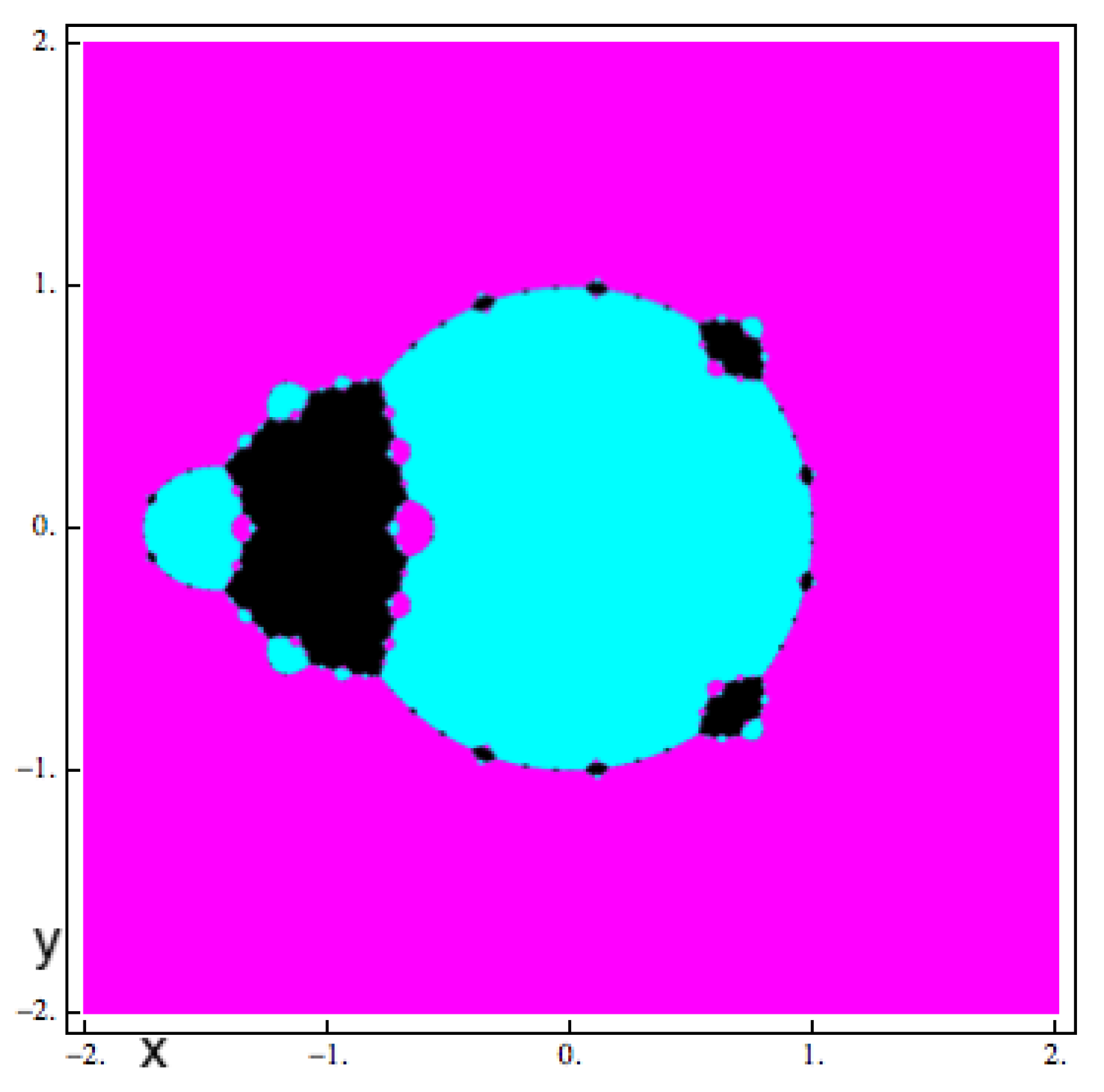
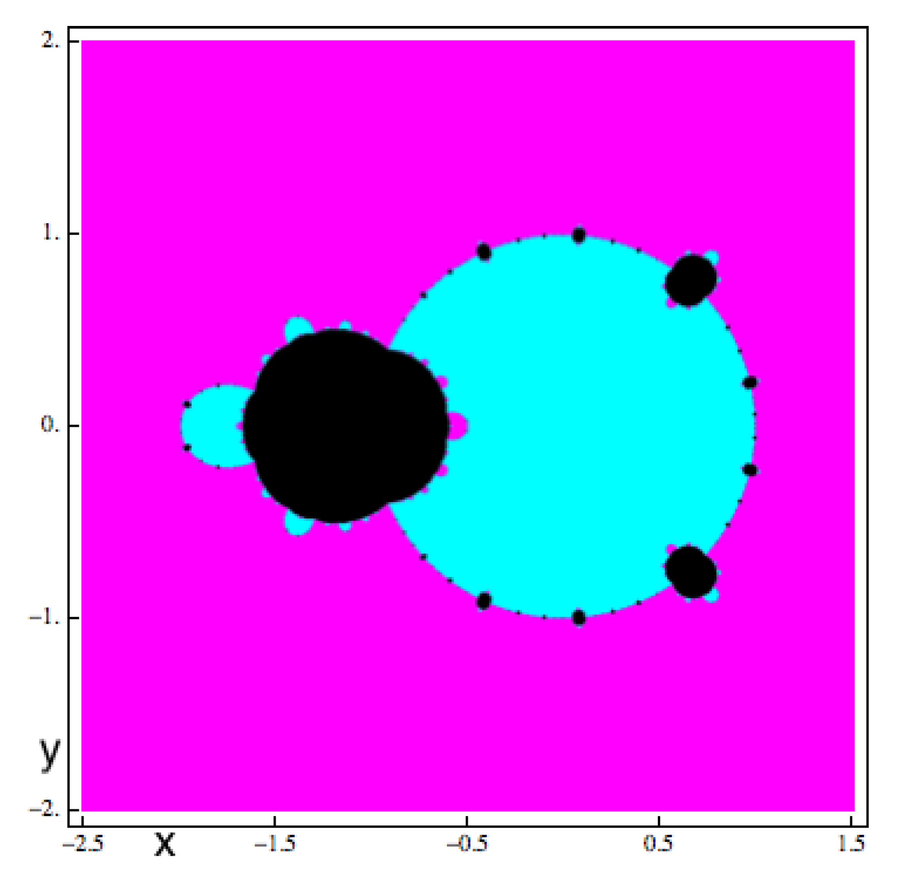
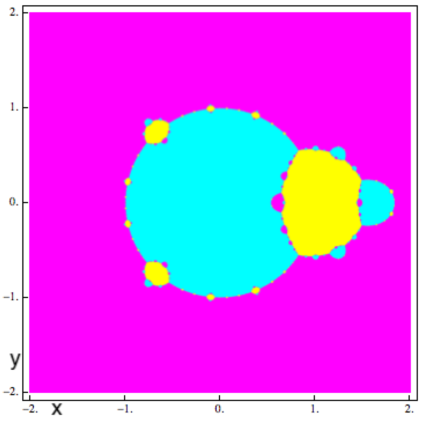
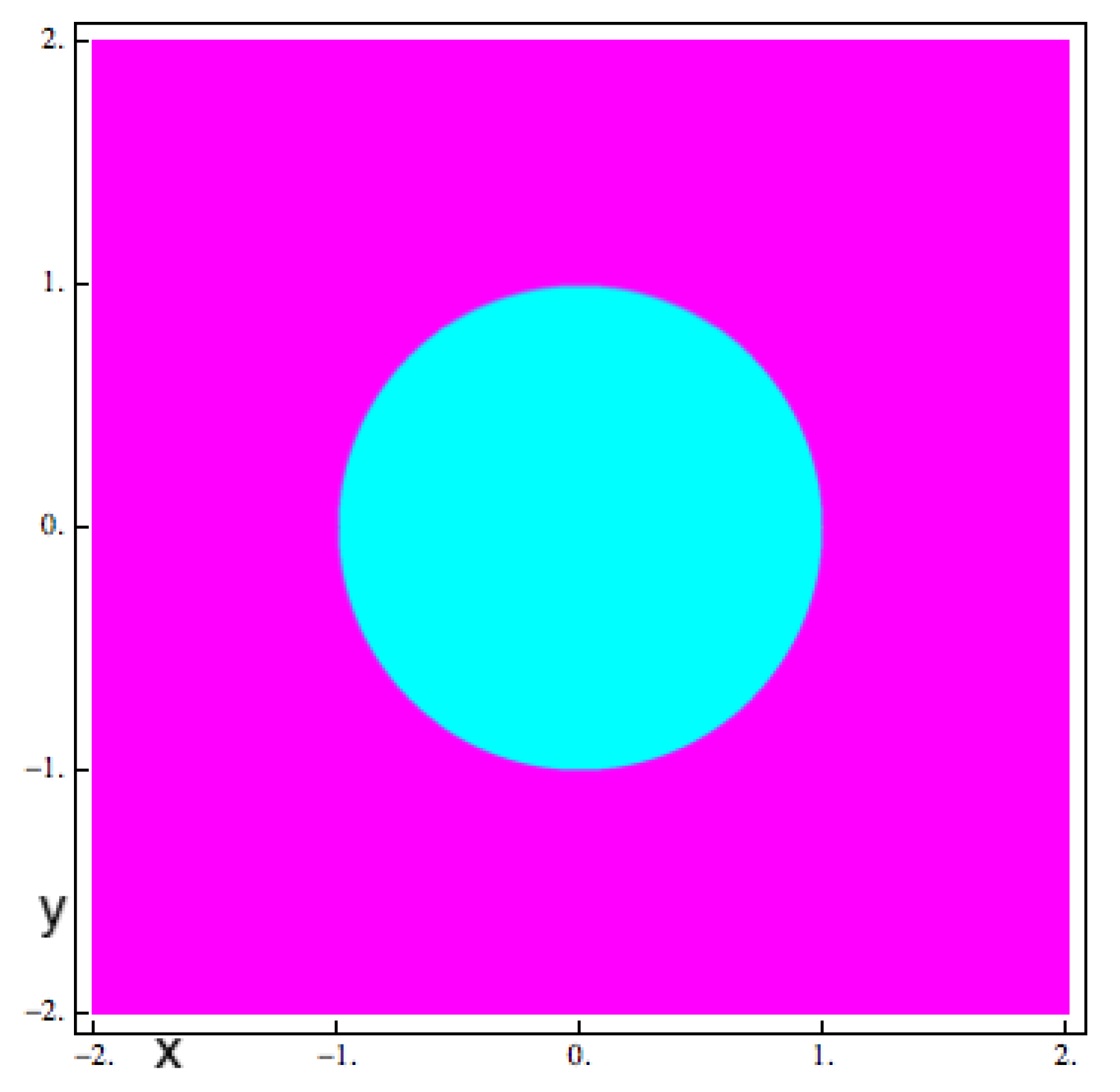
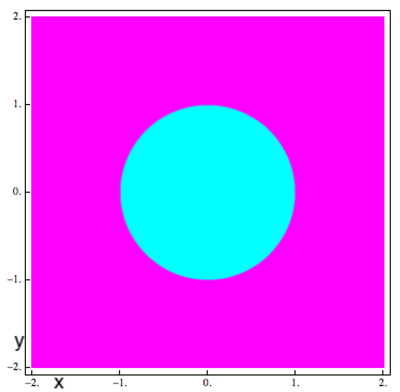
4. Dynamical Study

Here, we study the dynamical behavior of the operator associated to the bi-parametric scheme (3). On the one hand, the basins of attraction show us all the starting points that will converge to any root, if we apply an iterative method, so we can see in a visual way which points are good choices as a starting point and which are not. On the other hand, when we have a family of iterative methods, we cannot compute the basins of each member of the family since there exist infinitely many members, so we need to use another tool, this tool is the parameter plane. With this tool and using the definition of the critical point, we can characterize those members of the family that will have a good behavior in terms of stability and those who have complex behavior such as convergence to extraneous fixed points, cycles or even chaotical behavior. When the members of the family with “good” and “bad” behavior have been found, we can draw the basins in order to find the size of the “bad” zones. That is the reason why the study of dynamical behavior of a family of iterative methods is so important.

The basin of attraction of an attractor $x^{*}$ is defined as

$$\mathcal{A}\left(x^{*}\right)=\{z_0\in \widehat{\mathbb{C}}:R^n\left(z_0\right)\to x^{*},n\to \infty \}.$$

The Fatou set of rational function R, $\mathcal{F}\left(R\right)$, is defined as the set of points of the complex plane $z\in \widehat{\mathbb{C}}$ whose orbits converges to any attractor. Its complement set is the Julia set,$\mathcal{J}\left(R\right)$ in $\widehat{\mathbb{C}}$. This means that the attraction basins of any fixed point belongs to the Fatou set whereas the boundaries of these basins belong to the Julia set.

The complex dynamics of the family (3) is studied by applying the rational operator associated to the family on a generic polynomial $p\left(z\right)=(z-a)(z-b)$, and by using the Möebius map $h\left(z\right)=\frac{z-a}{z-b}$, whose properties are

$$i)h\left(\infty \right)=1,ii)h\left(a\right)=0,iii)h\left(b\right)=\infty .$$

The rational operator associated with the proposed family of iterative methods (3) (we call it $F\left(z\right)$) is obtained by using $p\left(z\right)$ and is given by

$$\begin{array}{c}G(z,r,t)=h\circ F\circ h^{-1}\left(z\right)=\frac{z^4\left(9r^{2}z+9r^2+6rtz-18rt-3t^{2}z-11t^2\right)}{9r^{2}z+9r^2-18rtz+6rt-11t^{2}z-3t^2}.\hfill \end{array}$$

(52)

4.1. Fixed Points and Stability

Note that $z=0$ and $z=\infty$ are fixed points of $G(z,r,t)$ that are related to the roots of the polynomial $p\left(z\right)$. We focus our attention on the extraneous fixed points, i.e., the points which are fixed points of G and are not solutions of the equation $F\left(z\right)=0$. Notice that $z=1$ is an extraneous fixed point, associated to infinity. Moreover, we find the following extraneous fixed points:

$$\begin{array}{ccc}e{x}_1(r,t)\hfill & =& -1,\hfill \\ e{x}_2(r,t)\hfill & =& \frac{-9r^2-\sqrt{-243r^4-756r^{3}t+198r^2{t}^2+540r{t}^3+85t^4}+18rt+11t^2}{6\left(3r^2+2rt-t^2\right)},\hfill \\ e{x}_3(r,t)\hfill & =& \frac{-9r^2+\sqrt{-243r^4-756r^{3}t+198r^2{t}^2+540r{t}^3+85t^4}+18rt+11t^2}{6\left(3r^2+2rt-t^2\right)}.\hfill \end{array}$$

Related to the stability of these extraneous fixed points we need $G^{\prime }$, which is given as

$$\begin{array}{c}{G}^{\prime }(z,r,t)=\frac{12z^3\left(27r^4{(z+1)}^2-36r^{3}t\left(z^2+z+1\right)-6r^2{t}^2(z(13z-4)+13)-4r{t}^3((z-21)z+1)+t^4(z(11z+34)+11)\right)}{{\left(9r^2(z+1)+6rt(1-3z)-t^2(11z+3)\right)}^2}.\hfill \end{array}$$

From the form of the derivative, it is clear that the origin and ∞ are superattractive fixed points for every value of r and t.

Related to the stability of the other fixed points, we obtain the multiplicators associated to each one as:

$$\begin{array}{ccc}{G}^{\prime }(e{x}_1(r,t),r,t)\hfill & =& \frac{3}{4}\left(r\left(\frac{4}{3r+t}+\frac{1}{t}\right)+3\right),\hfill \\ G^{\prime }(e{x}_2(r,t),r,t)\hfill & =& \frac{4\left(81r^4+216r^{3}t-54r^2{t}^2-144r{t}^3-19t^4\right)}{9{(t-3r)}^2{(r+t)}^2},\hfill \\ G^{\prime }(e{x}_3(r,t),r,t)\hfill & =& \frac{4\left(81r^4+216r^{3}t-54r^2{t}^2-144r{t}^3-19t^4\right)}{9{(t-3r)}^2{(r+t)}^2}.\hfill \end{array}$$

Due to the complexity of the stability function of the extraneous fixed points, we use the graphical tools of software Mathematica to obtain the regions of stability of them. In Figure 1 and Figure 2, the stability regions of $z=-1$, $e{x}_2(r,t)$ (and also $e{x}_3(r,t)$ since its behavior is similar to $e{x}_2(r,t)$ as both points are conjugated) are shown. Every value of the parameter which is in grey means that the associated fixed point is repulsor.

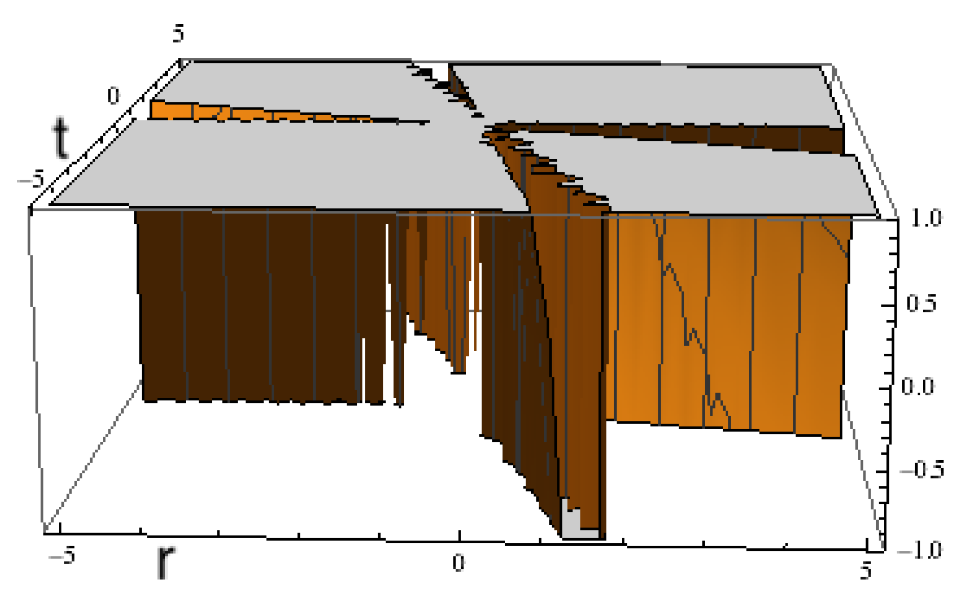
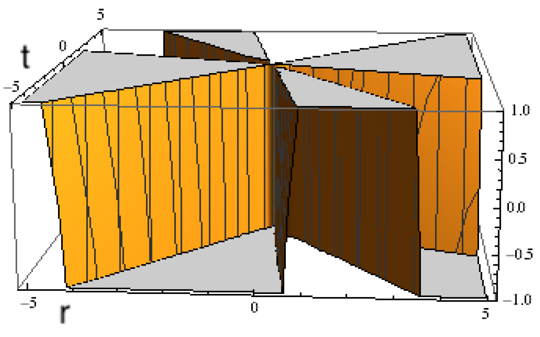
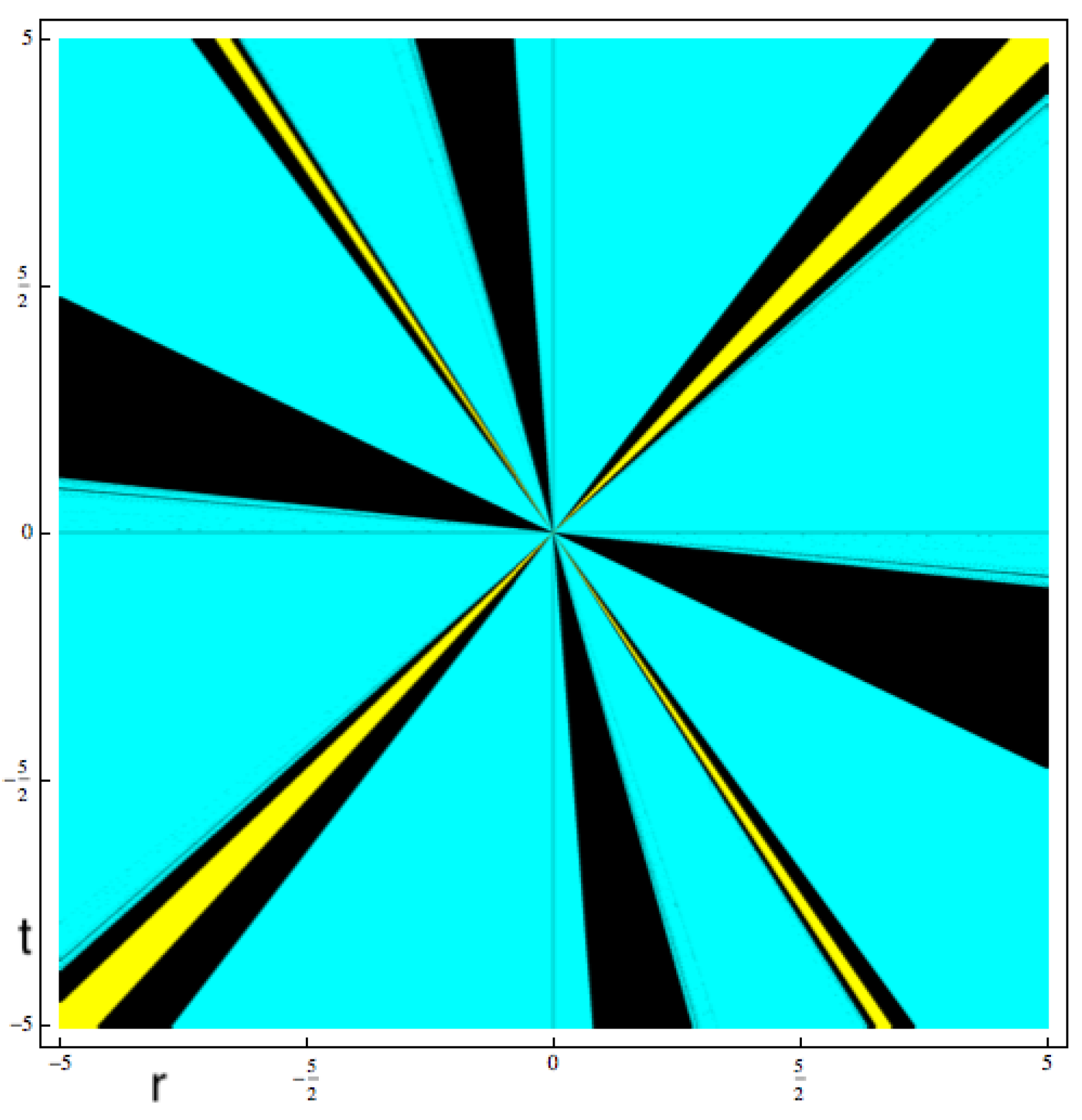
4.2. Critical Points and Parameter Spaces

Here, the critical points will be calculated and the convergence planes, which correspond to the parameter planes, associated to the free critical points will be shown. We obtain that $z=0$ and $z=\infty$ are critical points. On the other hand, the free critical points are the following:

$$c{r}_0=-1,$$

$$\begin{array}{c}c{r}_1(r,t)=-\frac{27r^4-18r^{3}t+12r^2{t}^2+2\sqrt{t(r-t)(3r+t)(3r+2t)\left(9r^2-6rt-7t^2\right)\left(3r^2+14rt+3t^2\right)}+42r{t}^3+17t^4}{(3r-t)(r+t)\left(9r^2-18rt-11t^2\right)}\hfill \end{array}$$

and

$$\begin{array}{c}c{r}_2(r,t)=\frac{-27r^4+18r^{3}t-12r^2{t}^2+2\sqrt{t(r-t)(3r+t)(3r+2t)\left(9r^2-6rt-7t^2\right)\left(3r^2+14rt+3t^2\right)}-42r{t}^3-17t^4}{(3r-t)(r+t)\left(9r^2-18rt-11t^2\right)}.\hfill \end{array}$$

We present the following results involving the free critical points.

Lemma 1.

(a)

If $r=-\frac{1}{3}\left(2t\right)$ or $r=\frac{1}{3}\left(2\sqrt{2}t+t\right)$ or $r=\frac{1}{3}\left(t-2\sqrt{2}t\right)$, then $c{r}_1=c{r}_2=1$.

(b)

If $r=\frac{1}{3}\left(2\sqrt{10}t-7t\right)$ or $r=\frac{1}{3}\left(-2\sqrt{10}t-7t\right)$ or $t=0$, then $c{r}_1=c{r}_2=-1$.

(c)

For other values of r and t, the family has 2 free critical points.

Moreover, it is clear that for every value of r and t, $c{r}_1(r,t)=\frac{1}{c{r}_2(r,t)}$

We will only study the parameter planes associated to the other two free critical points because the behavior of $c{r}_0(r,t)=-1$ is simple due to the fact that it is a pre-image of the extraneous fixed point $z=1$ related to the original divergence to ∞. In order to study the behavior of these free critical points, we are going to draw the parameter planes but we will use a variant of the algorithms proposed in [27], in which we consider the horizontal axis as the r-axis and the vertical as the t-axis, and iterate the associated free critical point. In the parameter plane, dit appears in cyan the convergence to 0 and to ∞, in yellow the convergence to 1 and in black the convergence to any point or cycle distinct to the roots or even divergence or chaos. Consequently, by just looking at the parameter plane, we can see which pair of points $(r,t)$ will have a desirable behavior in terms of stability, every point in cyan is a good choice.

In Figure 3, the parameter plane associated to $c{r}_2(r,t)$ is shown, where some zones with anomalies are detected.

Now, we will draw some of the dynamical planes. The way we draw these is the following: each point represents a point of the complex plane in the form $z=x+yI$ and we iterate that point a maximum of 1000 iterations and draw the convergence to 0 in magenta, to ∞ in cyan, whereas non-convergence to the roots in black color. First of all, in Figure 4 and Figure 5 appear two dynamical planes associated with non-convergent zones. On the other hand, in Figure 6, a dynamical plane with regions of convergence to $z=1$, is shown.

Finally, we show the planes without any chaos. In Figure 7 appears the dynamical plane associated without non-convergence problem whereas in Figure 8 appears the plane associated to special case the Jarratt’s method of the family.

5. Numerical Examples

Here, we shall demonstrate the theoretical results of local convergence which we have proved in Section 3. Results are also compared with that of Newton’s method. The radius of convergence $\left(s_N\right)$ for Newton’s method is given by

$$s_N=\frac{2}{2L_0+L},$$

(53)

where $L_0$ and L are given parameters (see [1,25]).

We consider three numerical examples.

Example 1.

Let us consider $B={\mathbb{R}}^{m-1}$ for natural integer $m\ge 2$. B is equipped with the max-norm $\parallel x\parallel$$={\max }_{1\le i\le m-1}\parallel x_i\parallel$. The corresponding matrix norm is $\parallel A\parallel ={\max }_{1\le i\le m-1}{\sum }_{j=1}^{j=m-1}\left|a_{ij}\right|$ for $A=$${\left(a_{ij}\right)}_{1\le i,j\le m-1}$. Consider the following two point boundary value problem on interval [0, 1] is

$$\left\{\begin{array}{c}{v}^{″}+v^{3/2}=0,\hfill \\ v\left(0\right)=v\left(1\right)=0.\hfill \end{array}\right.$$

(54)

Let us denote $h=1/m$, $u_i=hi$ and $v_i=v\left(u_i\right)$ for each $i=0,1,\dots ,m$. We can write the discretization of $v^{″}$ at points $u_i$ in the following form:

$$v_i^{″}\simeq \frac{v_{i-1}-2v_i+v_{i+1}}{h^2}\mathrm{for}\mathrm{each}i=2,3,\dots ,m-1.$$

Using the initial conditions in (54), we get that $v_0=v_m=0$ and (54) is equivalent to the system of nonlinear equation $F\left(v\right)=0$, where $v={(v_1,v_2,\dots ,v_{m-1})}^T$ and $F\left(v\right)$ is;

$$F\left(v\right)=\left\{\begin{array}{c}{h}^2{v}_1^{3/2}-2v_1+v_2,\hfill \\ v_{i-1}+h^2{v}_i^{3/2}-2v_i+v_{i+1}\mathrm{for}\mathrm{each}i=2,3,\dots ,m-1.\hfill \end{array}\right.$$

The Fréchet-derivative of operator F is given by

$$F^{\prime }\left(v\right)=\left(\begin{array}{ccccc}\frac{3}{2}{h}^2{v}_1^{1/2}-2& 1& 0& \dots & 0\\ 1& \frac{3}{2}{h}^2{v}_1^{1/2}-2& 1& \ddots & 0\\ 0& 1& \ddots & \ddots & ⋮\\ ⋮& \ddots & \ddots & \ddots & 1\\ 0& \dots & 0& 1& \frac{3}{2}{h}^2{v}_1^{1/2}-2\end{array}\right).$$

We choose $m=11$ and corresponding solution is $x^{*}={(0,0,\cdots ,0)}^T$. Then, we have that ${\varphi }_0\left(t\right)=\varphi \left(t\right)=L_{0}t$, $\psi \left(t\right)=Lt$, where $L_0=L=3.942631477$. Values of the parameters $s_N$, $s_1$, $s_2$ and $s^{*}$, using their definition, are given in

Table 1. Numerical results for Example 1.

Parameter	NM	JM	MI	MII	MIII	MIV
$s_N$	$0.169092$	-	-	-	-	-
$s_1$	-	$0.152183$	$0.152183$	$0.152183$	$0.152183$	$0.152183$
$s_2$	-	$0.114471$	$0.102803$	$0.0405032$	$0.102462$	$0.107633$
$s^{*}$	-	$0.114471$	$0.102803$	$0.0405032$	$0.102462$	$0.107633$

.

Thus the convergence of the method (3) is guaranteed, provided that $x_0\in U(x^{*},s^{*})$.

Example 2.

Let $B=C[0,1]$, be a space of continuous functions defined on $[0,1]$ and equipped with max norm. Let $\Omega =\overline{U}(0,1)$. Define F on Ω by

$$F\left(\phi \right)\left(x\right)=\varphi \left(x\right)-5{\int }_0^{1}x\theta \phi {\left(\theta \right)}^{3}d\theta .$$

We obtain that

$$F^{\prime }\left(\phi \left(\xi \right)\right)\left(x\right)=\xi \left(x\right)-15{\int }_0^{1}x\theta \phi {\left(\theta \right)}^2\xi \left(\theta \right)d\theta ,\mathrm{for}\mathrm{each}\xi \in \Omega .$$

Then, we have that ${\varphi }_0\left(t\right)=\varphi \left(t\right)=L_{0}t$ and $\psi \left(t\right)=Lt$, where $L_0=7.5$, $L=15$. Using the definition of $s_N$, $s_1$, $s_2$ and $s^{*}$, the parameter values are shown in

Table 2. Numerical results for Example 2.

Parameter	NM	JM	MI	MII	MIII	MIV
$s_N$	$0.0666667$	-	-	-	-	-
$s_1$	-	$0.0627273$	$0.0627273$	$0.0627273$	$0.0627273$	$0.0627273$
$s_2$	-	$0.0438191$	$0.0382687$	$0.0207147$	$0.0372223$	$0.0400211$
$s^{*}$	-	$0.0438191$	$0.0382687$	$0.0207147$	$0.0372223$	$0.0400211$

.

Therefore, the convergence of the method (3) to $x^{*}=0$ is guaranteed, provided that $x_0\in U(x^{*},s^{*})$.

Example 3.

Consider the nonlinear integral equation of the mixed Hammerstein-type [32] defined by

$$x\left(s\right)={\int }_0^{1}G(s,t)\left(x{\left(t\right)}^{3/2}+\frac{x{\left(t\right)}^2}{2}\right)dt,$$

(55)

where G is the Green’s function defined on the interval $[0,1]\times [0,1]$ by

$$G(s,t)=\left\{\begin{array}{c}(1-s)t,t\le s,\hfill \\ s(1-t),s\le t.\hfill \end{array}\right.$$

The solution of Equation (55) is $x^{*}\left(s\right)=0$, wherein $F:\Omega \subseteq C[0,1]\to C[0,1]$ is defined by

$$F\left(x\right)\left(s\right)=x\left(s\right)-{\int }_0^{1}G(s,t)\left(x{\left(t\right)}^{3/2}+\frac{x{\left(t\right)}^2}{2}\right)dt.$$

Observe that

$$\parallel {\int }_0^{1}G(s,t)dt\parallel \le \frac{1}{8}.$$

Then, we have that

$$F^{\prime }\left(x\right)y\left(s\right)=y\left(s\right)-{\int }_0^{1}G(s,t)\left(\frac{3}{2}x{\left(t\right)}^{1/2}+x\left(t\right)\right)dt,$$

so since $F^{\prime }\left(x^{*}\left(s\right)\right)=I$, then

$$\parallel F^{\prime }{\left(x^{*}\right)}^{-1}(F^{\prime }\left(x\right)-F^{\prime }\left(y\right))\parallel \le \frac{5}{16}\parallel x-y\parallel .$$

(56)

In (56), replacing y by $x_0$ we get that

$$\parallel F^{\prime }{\left(x^{*}\right)}^{-1}(F^{\prime }\left(x\right)-F^{\prime }\left(x_0\right))\parallel \le \frac{5}{16}\parallel x-x_0\parallel .$$

Therefore, we have

$${\varphi }_0\left(t\right)=\varphi \left(t\right)=L_{0}t\mathrm{and}\psi \left(t\right)=Lt,\mathrm{where}{L}_0=L=\frac{5}{16}.$$

Computed values of the parameters $s_N$, $s_1$, $s_2$, and $s^{*}$ are displayed in

Table 3. Numerical results for Example 3.

Parameter	NM	JM	MI	MII	MIII	MIV
$s_N$	$2.133333$	-	-	-	-	-
$s_1$	-	$1.920000$	$1.920000$	$1.920000$	$1.920000$	$1.920000$
$s_2$	-	$1.444421$	$1.297012$	$0.511010$	$1.292725$	$1.357911$
$s^{*}$	-	$1.444421$	$1.297012$	$0.511010$	$1.292725$	$1.357911$

.

Thus the convergence of the method (3) to $x^{*}\left(s\right)=0$ is guaranteed, provided that $x_0\in U(x^{*},s^{*})$.

We conclude that $s_N$ is larger than the new radii as expected because as the order of convergence increases the radius decreases in general.

6. Applications

The methods JM, MI, MII, MIII, and MIV of the family (3) are applied to solve different systems of nonlinear equations in ${\mathbb{R}}^m$. We also compare the methods with some existing fourth order methods. For instance, we choose the methods proposed by Babajee et al. [10], Cordero et al. [13], Darvishi-Barati [14], Hueso et al. [17], Noor-Noor [18], and Sharma-Arora [19], which are given by

Method by Babajee et al. (BM):

$$\begin{array}{cc}\hfill y_n=& x_n-\frac{2}{3}{F}^{\prime }{\left(x_n\right)}^{-1}F\left(x_n\right),\hfill \\ x_{n+1}=\hfill & x_n-2\left[I-\frac{1}{4}\left(F^{\prime }{\left(x_n\right)}^{-1}{F}^{\prime }\left(y_n\right)-I\right)+\frac{3}{4}{\left(F^{\prime }{\left(x_n\right)}^{-1}{F}^{\prime }\left(y_n\right)-I\right)}^2\right]\hfill \\ & \times {\left(F^{\prime }\left(x_n\right)+F^{\prime }\left(y_n\right)\right)}^{-1}F\left(x_n\right).\hfill \end{array}$$

Method by Cordero et al. (CM):

$$\begin{array}{cc}\hfill y_n=& x_n-F^{\prime }{\left(x_n\right)}^{-1}F\left(x_n\right),\hfill \\ \hfill x_{n+1}=& y_n-\left[2F^{\prime }{\left(x_n\right)}^{-1}-F^{\prime }{\left(x_n\right)}^{-1}{F}^{\prime }\left(y_n\right)F^{\prime }{\left(x_n\right)}^{-1})\right]F\left(y_n\right).\hfill \end{array}$$

Darvishi-Barati Method (DBM):

$$\begin{array}{cc}\hfill y_n=& x_n-F^{\prime }{\left(x_n\right)}^{-1}F\left(x_n\right),\hfill \\ \hfill z_n=& x_n-F^{\prime }{\left(x_n\right)}^{-1}\left(F\left(x_n\right)+F\left(y_n\right)\right),\hfill \\ \hfill x_{n+1}=& x_n-{\left[\frac{1}{6}{F}^{\prime }\left(x_n\right)+\frac{2}{3}{F}^{\prime }\left(\frac{x_n+z_n}{2}\right)+\frac{1}{6}{F}^{\prime }\left(z_n\right)\right]}^{-1}F\left(x_n\right).\hfill \end{array}$$

Method by Hueso et al. (HM):

$$\begin{array}{cc}\hfill y_n=& x_n-\theta {\Gamma }_{x_n}F\left(x_n\right),\hfill \\ \hfill H(x_n,y_n)=& {\Gamma }_{x_n}{F}^{\prime }\left(y_n\right),\hfill \\ \hfill G_s(x_n,y_n)=& s_{1}I+s_{2}H(y_n,x_n)+s_{3}H(x_n,y_n)+s_{4}H{(y_n,x_n)}^2\hfill \\ \hfill z_n=& x_n-G_s(x_n,y_n){\Gamma }_{x_n}F\left(x_n\right),\hfill \\ \hfill x_{n+1}=& z_n,\hfill \end{array}$$

where ${\Gamma }_{x_n}=F^{\prime }{\left(x_n\right)}^{-1}$, $\theta =\frac{2}{3}$, $s_1=\frac{5-8s_2}{8}$, $s_3=\frac{s_2}{3}$, $s_4=\frac{9-8s_2}{24}$ and $s_2\in \mathbb{R}$. In numerical problems, we choose $s_2=1$.

Noor-Noor Method(NNM):

$$\begin{array}{cc}\hfill y_n=& x_n-F^{\prime }{\left(x_n\right)}^{-1}F\left(x_n\right),\hfill \\ \hfill z_n=& -F^{\prime }{\left(x_n\right)}^{-1}F\left(y_n\right),\hfill \\ \hfill x_{n+1}=& x_n-F^{\prime }{\left(x_n\right)}^{-1}F\left(x_n\right)-F^{\prime }{\left(x_n\right)}^{-1}F\left(y_n\right)-F^{\prime }{\left(x_n\right)}^{-1}F(y_n+z_n).\hfill \end{array}$$

Sharma-Arora Method (SAM):

$$\begin{array}{cc}\hfill y_n=& x_n-\frac{2}{3}{F}^{\prime }{\left(x_n\right)}^{-1}F\left(x_n\right),\hfill \\ \hfill x_{n+1}=& x_n-\left[\frac{23}{8}I-F^{\prime }{\left(x_n\right)}^{-1}{F}^{\prime }\left(y_n\right)\left(3I-\frac{9}{8}{F}^{\prime }{\left(x_n\right)}^{-1}{F}^{\prime }\left(y_n\right)\right)\right]F^{\prime }{\left(x_n\right)}^{-1}F\left(x_n\right).\hfill \end{array}$$

The computations are performed in programming package Mathematica [33] with multiple-precision arithmetic using 4096 digits. Programs are performed in the processor, AMD A8-7410 APU with AMU Radeon R5 Graphics @ 2.20 GHz (64-bit Operating System) Microsoft Window 10 Ultimate 2016. In each method, we record the number of iterations $\left(n\right)$ that are required to converge to the solution by employing the stopping criterion

$$\left|\right|x_{n+1}-x_n\left|\right|+\left|\right|F\left(x_n\right)\left|\right|<{10}^{-200}.$$

The theoretical order of convergence is verified by calculating the approximate computational order of convergence (ACOC) using the formula (see [4])

$$\mathrm{ACOC}=\frac{ln(\parallel x_{n+1}-x_n\parallel /\parallel x_n-x_{n-1}\parallel )}{ln(\parallel x_n-x_{n-1}\parallel /\parallel x_{n-1}-x_{n-2}\parallel )}.$$

(57)

For numerical experiments we consider the following problems:

Problem 1.

Consider the nonlinear problem BROYDN3D [34]. Let $x={(x_1,x_2,\cdots ,x_m)}^T$. The nonlinear system $F\left(x\right)=0$ is given by $F={(F_1,F_2,\cdots ,F_m)}^T$ with

$$F_i\left(x\right)=(3-2x_i)x_i-x_{i-1}-2x_{i+1}+1,1\le i\le m$$

where $x_0=x_{m+1}=0$ by convention. The initial guess is $x^{\left(0\right)}={\{-1,-1\stackrel{m-times}{······},-1\}}^T$.

In tests, we choose the systems with dimension $m=10,50,100,200,500$ and their corresponding solutions are given by

$$\begin{array}{cc}\{\hfill & -0.7596\dots ,-0.7166\dots ,-0.7085\dots ,-0.7066\dots ,-0.7051\dots ,-0.7015\dots ,-0.6918\dots ,-0.6657\dots ,\hfill \\ & {-0.5960\dots ,-0.4164\dots \}}^T,\hfill \\ \{\hfill & -0.5707\dots ,-0.6819\dots ,-0.7024\dots ,-0.7062\dots ,-0.7069\dots ,-0.7070\dots ,-0.7071\dots ,\cdots \cdots \cdots ,\hfill \\ & -0.7071\dots ,-0.7070\dots ,-0.7070\dots ,-0.7070\dots ,-0.7068\dots ,-0.7063\dots ,-0.7050\dots ,-0.7015\dots ,\hfill \\ & {-0.6918\dots ,-0.6657\dots ,-0.5960\dots ,-0.4164\dots \}}^T,\hfill \\ \{\hfill & -0.5707\dots ,-0.6819\dots ,-0.7024\dots ,-0.7062\dots ,-0.7069\dots ,-0.7070\dots ,-0.7071\dots ,\cdots \cdots \cdots ,\hfill \\ & -0.7071\dots ,-0.7070\dots ,-0.7070\dots ,-0.7070\dots ,-0.7068\dots ,-0.7063\dots ,-0.7050\dots ,-0.7015\dots ,\hfill \\ & {-0.6918\dots ,-0.6657\dots ,-0.5960\dots ,-0.4164\dots \}}^T,\hfill \\ \{\hfill & -0.5707\dots ,-0.6819\dots ,-0.7024\dots ,-0.7062\dots ,-0.7069\dots ,-0.7070\dots ,-0.7071\dots ,-0.7071\dots ,\hfill \\ & -0.7071\dots ,\cdots \cdots \cdots ,-0.7071\dots ,-0.7070\dots ,-0.7070\dots ,-0.7070\dots ,-0.7068\dots ,\hfill \\ & {-0.7063\dots ,-0.7050\dots ,-0.7015\dots ,-0.6918\dots ,-0.6657\dots ,-0.5960\dots ,-0.4164\dots \}}^T\hfill \end{array}$$

and

$$\begin{array}{cc}\{\hfill & -0.5707\dots ,-0.6819\dots ,-0.7024\dots ,-0.7062\dots ,-0.7069\dots ,-0.7070\dots ,-0.7071\dots ,-0.7071\dots ,\hfill \\ & -0.7071\dots ,-0.7071\dots ,\cdots \cdots \cdots ,-0.7071\dots ,-0.7070\dots ,-0.7070\dots ,-0.7070\dots ,-0.7068\dots ,\hfill \\ & {-0.7063\dots ,-0.7050\dots ,-0.7015\dots ,-0.6918\dots ,-0.6657\dots ,-0.5960\dots ,-0.4164\dots \}}^T.\hfill \end{array}$$

Problem 2.

Considering the system of nonlinear equations [35]:

$$\left\{\begin{array}{c}{x}_i^2{x}_{i+1}-1,1\le i\le m-1,\hfill \\ x_i^2{x}_1-1,i=m.\hfill \end{array}\right.$$

with initial value $x^{\left(0\right)}={\{\frac{3}{2},\frac{3}{2},\stackrel{m-times}{\cdots },\frac{3}{2}\}}^T$ towards the required solution of the systems of equations for $m=10,50,100,200,500$. The corresponding solutions are: $x^{*}={(1,1\stackrel{10}{\cdots },1)}^T$, ${(1,1\stackrel{50}{\cdots },1)}^T$, ${(1,1\stackrel{100}{\cdots },1)}^T$, ${(1,1\stackrel{200}{\cdots },1)}^T$ and ${(1,1\stackrel{500}{\cdots },1)}^T$.

Problem 3.

Next, the boundary value problem (see [19]):

$$u^{″}+u^3=0,u\left(0\right)=0,u\left(1\right)=1,$$

is studied. Assume the following partitioning of the interval $[0,1]$:

$$t_0=0<t_1<t_2<\cdots <t_{l-1}<t_l=1,t_{j+1}=t_j+h,h=1/l.$$

Let us define $u_0=u\left(t_0\right)=0$, $u_1=u\left(t_1\right),...,u_{l-1}=u\left(t_{l-1}\right)$, $u_l=u\left(t_l\right)=1$. We discretize the problem by using the numerical formulae for first and second derivatives

$$u_k^{″}=\frac{u_{k-1}-2u_k+u_{k+1}}{h^2},(k=1,2,3\dots ,l-1),$$

then the following system of $l-1$ nonlinear equations in $l-1$ variables is obtained:

$$u_{k-1}-2u_k+u_{k+1}+h^2{u}_k^3=0,(k=1,2,3\dots ,l-1).$$

In particular, we solve this problem for $l=11,51,101,201,501$ so that $m=10,50,100,200,500$ by selecting $u^{\left(0\right)}={\{1,1,\stackrel{m-times}{\cdots },1\}}^T$ as the initial value. Their corresponding solutions are given as follows:

$$\begin{array}{cc}\{\hfill & {0.0959\dots ,0.1919\dots ,0.2878\dots ,0.3835\dots ,0.4787\dots ,0.5730\dots ,0.6658\dots ,0.7561\dots ,0.8429\dots ,0.9247\dots \}}^T,\hfill \end{array}$$

$$\begin{array}{cc}\{\hfill & 0.0207\dots ,0.0414\dots ,0.0621\dots ,0.0828\dots ,0.1035\dots ,0.1242\dots ,0.1449\dots ,0.1656\dots ,0.1863\dots ,0.2070\dots ,\hfill \\ & 0.2277\dots ,0.2484\dots ,0.2691\dots ,0.2898\dots ,0.3105\dots ,0.3312\dots ,0.3518\dots ,0.3724\dots ,0.3930\dots ,0.4136\dots ,\hfill \\ & 0.4342\dots ,0.4547\dots ,0.4752\dots ,0.4957\dots ,0.5161\dots ,0.5364\dots ,0.5567\dots ,0.5769\dots ,0.5971\dots ,0.6172\dots ,\hfill \\ & 0.6372\dots ,0.6570\dots ,0.6768\dots ,0.6965\dots ,0.7160\dots ,0.7354\dots ,0.7546\dots ,0.7737\dots ,0.7925\dots ,0.8112\dots ,\hfill \\ & {0.8297\dots ,0.8480\dots ,0.8660\dots ,0.8838\dots ,0.9013\dots ,0.9186\dots ,0.9355\dots ,0.9521\dots ,0.9684\dots ,0.9844\dots \}}^T,\hfill \end{array}$$

$$\begin{array}{cc}\{\hfill & 0.0104\dots ,0.0209\dots ,0.0313\dots ,0.0418\dots ,0.0522\dots ,0.0627\dots ,0.0732\dots ,0.0836\dots ,0.0941\dots ,0.1045\dots ,\hfill \\ & 0.1150\dots ,0.1255\dots ,0.1359\dots ,0.1464\dots ,0.1568\dots ,0.1673\dots ,0.1777\dots ,0.1882\dots ,0.1986\dots ,0.2091\dots ,\hfill \\ & 0.2196\dots ,0.2300\dots ,0.2405\dots ,0.2509\dots ,0.2614\dots ,0.2718\dots ,0.2822\dots ,0.2927\dots ,0.3031\dots ,0.3136\dots ,\hfill \\ & 0.3240\dots ,0.3344\dots ,0.3449\dots ,0.3553\dots ,0.3657\dots ,0.3761\dots ,0.3865\dots ,0.3969\dots ,0.4073\dots ,0.4177\dots ,\hfill \\ & 0.4281\dots ,0.4385\dots ,0.4488\dots ,0.4592\dots ,0.4695\dots ,0.4799\dots ,0.4902\dots ,0.5005\dots ,0.5108\dots ,0.5211\dots ,\hfill \\ & 0.5314\dots ,0.5417\dots ,0.5519\dots ,0.5621\dots ,0.5724\dots ,0.5826\dots ,0.5927\dots ,0.6029\dots ,0.6130\dots ,0.6231\dots ,\hfill \\ & 0.6332\dots ,0.6433\dots ,0.6533\dots ,0.6633\dots ,0.6733\dots ,0.6832\dots ,0.6932\dots ,0.7031\dots ,0.7129\dots ,0.7227\dots ,\hfill \\ & 0.7325\dots ,0.7422\dots ,0.7519\dots ,0.7616\dots ,0.7712\dots ,0.7808\dots ,0.7903\dots ,0.7998\dots ,0.8092\dots ,0.8186\dots ,\hfill \\ & 0.8279\dots ,0.8372\dots ,0.8464\dots ,0.8555\dots ,0.8646\dots ,0.8736\dots ,0.8826\dots ,0.8915\dots ,0.9003\dots ,0.9091\dots ,\hfill \\ & {0.9177\dots ,0.9263\dots ,0.9348\dots ,0.9433\dots ,0.9516\dots ,0.9599\dots ,0.9681\dots ,0.9762\dots ,0.9842\dots ,0.9921\dots \}}^T,\hfill \end{array}$$

$$\begin{array}{cc}\{\hfill & 0.005\dots ,0.01\dots ,0.01\dots ,0.02\dots ,0.02\dots ,0.03\dots ,0.03\dots ,0.04\dots ,0.04\dots ,0.05\dots ,0.05\dots ,0.06\dots ,\hfill \\ & 0.06\dots ,0.07\dots ,0.07\dots ,0.08\dots ,0.08\dots ,0.09\dots ,0.09\dots ,0.10\dots ,0.11\dots ,0.11\dots ,0.12\dots ,0.12\dots ,\hfill \\ & 0.13\dots ,0.13\dots ,0.14\dots ,0.14\dots ,0.15\dots ,0.15\dots ,0.16\dots ,0.16\dots ,0.17\dots ,0.17\dots ,0.18\dots ,0.18\dots ,\hfill \\ & 0.19\dots ,0.19\dots ,0.20\dots ,0.21\dots ,0.21\dots ,0.22\dots ,0.22\dots ,0.23\dots ,0.23\dots ,0.24\dots ,0.24\dots ,0.25\dots ,\hfill \\ & 0.25\dots ,0.26\dots ,0.26\dots ,0.27\dots ,0.27\dots ,0.28\dots ,0.28\dots ,0.29\dots ,0.29\dots ,0.30\dots ,0.30\dots ,0.31\dots ,\hfill \\ & 0.32\dots ,0.32\dots ,0.33\dots ,0.33\dots ,0.34\dots ,0.34\dots ,0.35\dots ,0.35\dots ,0.36\dots ,0.36\dots ,0.37\dots ,0.37\dots ,\hfill \\ & 0.38\dots ,0.38\dots ,0.39\dots ,0.39\dots ,0.40\dots ,0.40\dots ,0.41\dots ,0.41\dots ,0.42\dots ,0.43\dots ,0.43\dots ,0.44\dots ,\hfill \\ & 0.44\dots ,0.45\dots ,0.45\dots ,0.46\dots ,0.46\dots ,0.47\dots ,0.47\dots ,0.48\dots ,0.48\dots ,0.49\dots ,0.49\dots ,0.50\dots ,\hfill \\ & 0.50\dots ,0.51\dots ,0.51\dots ,0.52\dots ,0.52\dots ,0.53\dots ,0.53\dots ,0.54\dots ,0.54\dots ,0.55\dots ,0.55\dots ,0.56\dots ,\hfill \\ & 0.57\dots ,0.57\dots ,0.58\dots ,0.58\dots ,0.59\dots ,0.59\dots ,0.60\dots ,0.60\dots ,0.61\dots ,0.61\dots ,0.62\dots ,0.62\dots ,\hfill \\ & 0.63\dots ,0.63\dots ,0.64\dots ,0.64\dots ,0.65\dots ,0.65\dots ,0.66\dots ,0.66\dots ,0.67\dots ,0.67\dots ,0.68\dots ,0.68\dots ,\hfill \\ & 0.69\dots ,0.69\dots ,0.70\dots ,0.70\dots ,0.71\dots ,0.71\dots ,0.72\dots ,0.72\dots ,0.73\dots ,0.73\dots ,0.74\dots ,0.74\dots ,\hfill \\ & 0.75\dots ,0.75\dots ,0.76\dots ,0.76\dots ,0.77\dots ,0.77\dots ,0.77\dots ,0.78\dots ,0.78\dots ,0.79\dots ,0.79\dots ,0.80\dots ,\hfill \\ & 0.80\dots ,0.81\dots ,0.81\dots ,0.82\dots ,0.82\dots ,0.83\dots ,0.83\dots ,0.84\dots ,0.84\dots ,0.85\dots ,0.85\dots ,0.85\dots ,\hfill \\ & 0.86\dots ,0.86\dots ,0.87\dots ,0.87\dots ,0.88\dots ,0.88\dots ,0.89\dots ,0.89\dots ,0.89\dots ,0.90\dots ,0.90\dots ,0.91\dots ,\hfill \\ & 0.91\dots ,0.92\dots ,0.92\dots ,0.93\dots ,0.93\dots ,0.93\dots ,0.94\dots ,0.94\dots ,0.95\dots ,0.95\dots ,0.95\dots ,0.96\dots ,\hfill \\ & {0.96\dots ,0.97\dots ,0.97\dots ,0.98\dots ,0.98\dots ,0.98\dots ,0.99\dots ,0.99\}}^T\hfill \\ & \mathrm{and}\hfill \\ \{\hfill & 0.002\dots ,0.004\dots ,0.006\dots ,0.008\dots ,0.01\dots ,0.01\dots ,0.01\dots ,0.01\dots ,0.01\dots ,0.02\dots ,0.02\dots ,0.02\dots ,\hfill \\ & 0.02\dots ,0.029\dots ,0.03\dots ,0.03\dots ,0.03\dots ,0.03\dots ,0.04\dots ,0.042\dots ,0.04\dots ,0.04\dots ,0.04\dots ,0.05\dots ,\hfill \\ & 0.05\dots ,0.05\dots ,0.05\dots ,0.05\dots ,0.06\dots ,0.06\dots ,0.065\dots ,0.06\dots ,0.06\dots ,0.07\dots ,0.07\dots ,0.07\dots ,\hfill \\ & 0.07\dots ,0.08\dots ,0.08\dots ,0.08\dots ,0.08\dots ,0.08\dots ,0.09\dots ,0.09\dots ,0.09\dots ,0.09\dots ,0.09\dots ,0.10\dots ,\hfill \\ & 0.10\dots ,0.10\dots ,0.10\dots ,0.10\dots ,0.11\dots ,0.11\dots ,0.11\dots ,0.11\dots ,0.12\dots ,0.12\dots ,0.12\dots ,0.12\dots ,\hfill \\ & 0.12\dots ,0.13\dots ,0.13\dots ,0.13\dots ,0.13\dots ,0.13\dots ,0.14\dots ,0.14\dots ,0.14\dots ,0.14\dots ,0.14\dots ,0.15\dots ,\hfill \\ & 0.15\dots ,0.15\dots ,0.15\dots ,0.16\dots ,0.16\dots ,0.16\dots ,0.16\dots ,0.16\dots ,0.17\dots ,0.17\dots ,0.17\dots ,0.17\dots ,\hfill \\ & 0.17\dots ,0.18\dots ,0.18\dots ,0.18\dots ,0.18\dots ,0.18\dots ,0.19\dots ,0.19\dots ,0.19\dots ,0.19\dots ,0.20\dots ,0.20\dots ,\hfill \\ & 0.20\dots ,0.20\dots ,0.20\dots ,0.21\dots ,0.21\dots ,0.21\dots ,0.21\dots ,0.21\dots ,0.22\dots ,0.22\dots ,0.22\dots ,0.22\dots ,\hfill \\ & 0.22\dots ,0.23\dots ,0.23\dots ,0.23\dots ,0.23\dots ,0.24\dots ,0.24\dots ,0.24\dots ,0.24\dots ,0.24\dots ,0.25\dots ,0.25\dots ,\hfill \\ & 0.25\dots ,0.25\dots ,0.25\dots ,0.26\dots ,0.26\dots ,0.26\dots ,0.26\dots ,0.26\dots ,0.27\dots ,0.27\dots ,0.27\dots ,0.27\dots ,\hfill \\ & 0.28\dots ,0.28\dots ,0.28\dots ,0.28\dots ,0.28\dots ,0.29\dots ,0.29\dots ,0.29\dots ,0.29\dots ,0.29\dots ,0.30\dots ,0.30\dots ,\hfill \end{array}$$

$$\begin{array}{c}0.30\dots ,0.30\dots ,0.30\dots ,0.31\dots ,0.31\dots ,0.31\dots ,0.31\dots ,0.32\dots ,0.32\dots ,0.32\dots ,0.32\dots ,0.32\dots ,\hfill \\ 0.33\dots ,0.33\dots ,0.33\dots ,0.33\dots ,0.33\dots ,0.34\dots ,0.34\dots ,0.34\dots ,0.34\dots ,0.34\dots ,0.35\dots ,0.35\dots ,\hfill \\ 0.35\dots ,0.35\dots ,0.36\dots ,0.36\dots ,0.36\dots ,0.36\dots ,0.36\dots ,0.37\dots ,0.37\dots ,0.37\dots ,0.37\dots ,0.37\dots ,\hfill \\ 0.38\dots ,0.38\dots ,0.38\dots ,0.38\dots ,0.38\dots ,0.39\dots ,0.39\dots ,0.39\dots ,0.39\dots ,0.40\dots ,0.40\dots ,0.40\dots ,\hfill \\ 0.40\dots ,0.40\dots ,0.41\dots ,0.41\dots ,0.41\dots ,0.41\dots ,0.41\dots ,0.42\dots ,0.42\dots ,0.42\dots ,0.42\dots ,0.42\dots ,\hfill \\ 0.43\dots ,0.43\dots ,0.43\dots ,0.43\dots ,0.43\dots ,0.44\dots ,0.44\dots ,0.44\dots ,0.44\dots ,0.45\dots ,0.45\dots ,0.45\dots ,\hfill \\ 0.45\dots ,0.45\dots ,0.46\dots ,0.46\dots ,0.46\dots ,0.46\dots ,0.46\dots ,0.47\dots ,0.47\dots ,0.47\dots ,0.47\dots ,0.47\dots ,\hfill \\ 0.48\dots ,0.48\dots ,0.48\dots ,0.48\dots ,0.48\dots ,0.49\dots ,0.49\dots ,0.49\dots ,0.49\dots ,0.50\dots ,0.50\dots ,0.50\dots ,\hfill \\ 0.50\dots ,0.50\dots ,0.51\dots ,0.51\dots ,0.51\dots ,0.51\dots ,0.51\dots ,0.52\dots ,0.52\dots ,0.52\dots ,0.52\dots ,0.52\dots ,\hfill \\ 0.53\dots ,0.53\dots ,0.53\dots ,0.53\dots ,0.53\dots ,0.54\dots ,0.54\dots ,0.54\dots ,0.54\dots ,0.55\dots ,0.55\dots ,0.55\dots ,\hfill \\ 0.55\dots ,0.55\dots ,0.56\dots ,0.56\dots ,0.56\dots ,0.56\dots ,0.56\dots ,0.57\dots ,0.57\dots ,0.57\dots ,0.57\dots ,0.57\dots ,\hfill \\ 0.58\dots ,0.58\dots ,0.58\dots ,0.58\dots ,0.58\dots ,0.59\dots ,0.59\dots ,0.59\dots ,0.59\dots ,0.59\dots ,0.60\dots ,0.60\dots ,\hfill \\ 0.60\dots ,0.60\dots ,0.60\dots ,0.61\dots ,0.61\dots ,0.61\dots ,0.61\dots ,0.61\dots ,0.62\dots ,0.62\dots ,0.62\dots ,0.62\dots ,\hfill \\ 0.63\dots ,0.63\dots ,0.63\dots ,0.63\dots ,0.63\dots ,0.64\dots ,0.64\dots ,0.64\dots ,0.64\dots ,0.64\dots ,0.65\dots ,0.65\dots ,\hfill \\ 0.65\dots ,0.65\dots ,0.65\dots ,0.66\dots ,0.66\dots ,0.66\dots ,0.66\dots ,0.66\dots ,0.67\dots ,0.67\dots ,0.67\dots ,0.67\dots ,\hfill \\ 0.67\dots ,0.68\dots ,0.68\dots ,0.68\dots ,0.68\dots ,0.68\dots ,0.69\dots ,0.69\dots ,0.69\dots ,0.69\dots ,0.69\dots ,0.70\dots ,\hfill \\ 0.70\dots ,0.70\dots ,0.70\dots ,0.70\dots ,0.71\dots ,0.71\dots ,0.71\dots ,0.71\dots ,0.71\dots ,0.72\dots ,0.72\dots ,0.72\dots ,\hfill \\ 0.72\dots ,0.72\dots ,0.73\dots ,0.73\dots ,0.73\dots ,0.73\dots ,0.73\dots ,0.74\dots ,0.74\dots ,0.74\dots ,0.74\dots ,0.74\dots ,\hfill \\ 0.74\dots ,0.75\dots ,0.75\dots ,0.75\dots ,0.75\dots ,0.75\dots ,0.76\dots ,0.76\dots ,0.76\dots ,0.76\dots ,0.76\dots ,0.77\dots ,\hfill \\ 0.77\dots ,0.77\dots ,0.77\dots ,0.77\dots ,0.78\dots ,0.78\dots ,0.78\dots ,0.78\dots ,0.78\dots ,0.79\dots ,0.79\dots ,0.79\dots ,\hfill \\ 0.79\dots ,0.79\dots ,0.80\dots ,0.80\dots ,0.80\dots ,0.80\dots ,0.80\dots ,0.80\dots ,0.81\dots ,0.81\dots ,0.81\dots ,0.81\dots ,\hfill \\ 0.81\dots ,0.82\dots ,0.82\dots ,0.82\dots ,0.82\dots ,0.82\dots ,0.83\dots ,0.83\dots ,0.83\dots ,0.83\dots ,0.83\dots ,0.83\dots ,\hfill \\ 0.84\dots ,0.84\dots ,0.84\dots ,0.84\dots ,0.84\dots ,0.85\dots ,0.85\dots ,0.85\dots ,0.85\dots ,0.85\dots ,0.85\dots ,0.86\dots ,\hfill \\ 0.86\dots ,0.86\dots ,0.86\dots ,0.86\dots ,0.87\dots ,0.87\dots ,0.87\dots ,0.87\dots ,0.87\dots ,0.87\dots ,0.88\dots ,0.88\dots ,\hfill \\ 0.88\dots ,0.88\dots ,0.88\dots ,0.89\dots ,0.89\dots ,0.89\dots ,0.89\dots ,0.89\dots ,0.89\dots ,0.90\dots ,0.90\dots ,0.90\dots ,\hfill \\ 0.90\dots ,0.90\dots ,0.91\dots ,0.91\dots ,0.91\dots ,0.91\dots ,0.91\dots ,0.91\dots ,0.92\dots ,0.92\dots ,0.92\dots ,0.92\dots ,\hfill \\ 0.92\dots ,0.92\dots ,0.93\dots ,0.93\dots ,0.93\dots ,0.93\dots ,0.93\dots ,0.93\dots ,0.94\dots ,0.94\dots ,0.94\dots ,0.94\dots ,\hfill \\ 0.94\dots ,0.94\dots ,0.95\dots ,0.95\dots ,0.95\dots ,0.95\dots ,0.95\dots ,0.95\dots ,0.96\dots ,0.96\dots ,0.96\dots ,0.96\dots ,\hfill \\ 0.96\dots ,0.96\dots ,0.97\dots ,0.97\dots ,0.97\dots ,0.97\dots ,0.97\dots ,0.97\dots ,0.98\dots ,0.98\dots ,0.98\dots ,0.98\dots ,\hfill \\ {0.98\dots ,0.98\dots ,0.99\dots ,0.99\dots ,0.99\dots ,0.99\dots ,0.99\dots ,0.99\dots \}}^T.\hfill \end{array}$$

Numerical results are displayed in

Table 4. Comparison of performance of methods for Problem 1.

Methods	BM	CM	DBM	HM	NNM	SAM	JM	MI	MII	MIII	MIV
m = 10
n	5	5	5	5	5	5	5	5	5	5	5
$\parallel x_{n+1}-x_n\parallel$	$4.09(-124)$	$1.49(-116)$	$1.21(-140)$	$6.83(-137)$	$1.01(-121)$	$1.49(-116)$	$4.28(-158)$	$2.54(-146)$	$1.22(-142)$	$2.96(-130)$	$4.16(-200)$
ACOC	4.001	4.001	4.001	4.001	4.001	4.001	4.001	4.001	4.001	4.000	4.000
m = 50
n	5	5	5	5	5	5	5	5	5	5	5
$\parallel x_{n+1}-x_n\parallel$	$4.09(-124)$	$1.49(-116)$	$1.21(-140)$	$6.83(-137)$	$1.01(-121)$	$1.49(-116)$	$4.28(-158)$	$2.54(-146)$	$1.22(-142)$	$2.96(-130)$	$4.16(-200)$
ACOC	4.001	4.001	4.001	4.001	4.001	4.001	4.001	4.001	4.001	4.000	4.000
m = 100
n	5	5	5	5	5	5	5	5	5	5	5
$\parallel x_{n+1}-x_n\parallel$	$4.09(-124)$	$1.49(-116)$	$1.21(-140)$	$6.83(-137)$	$1.01(-121)$	$1.49(-116)$	$4.28(-158)$	$2.54(-146)$	$1.22(-142)$	$2.96(-130)$	$4.16(-200)$
ACOC	4.001	4.001	4.001	4.001	4.001	4.001	4.001	4.001	4.001	4.000	4.000
m = 200
n	5	5	5	5	5	5	5	5	5	5	5
$\parallel x_{n+1}-x_n\parallel$	$4.09(-124)$	$1.49(-116)$	$1.21(-140)$	$6.83(-137)$	$1.01(-121)$	$1.49(-116)$	$4.28(-158)$	$2.54(-146)$	$1.22(-142)$	$2.96(-130)$	$4.16(-200)$
ACOC	4.001	4.001	4.001	4.001	4.001	4.001	4.001	4.001	4.001	4.000	4.000
m = 500
n	5	5	5	5	5	5	5	5	5	5	5
$\parallel x_{n+1}-x_n\parallel$	$4.09(-124)$	$1.49(-116)$	$1.21(-140)$	$6.83(-137)$	$1.01(-121)$	$1.49(-116)$	$4.28(-158)$	$2.54(-146)$	$1.22(-142)$	$2.96(-130)$	$4.16(-200)$
ACOC	4.001	4.001	4.001	4.001	4.001	4.001	4.001	4.001	4.001	4.000	4.000

,

Table 5. Comparison of performance of methods for Problem 2.

Methods	BM	CM	DBM	HM	NNM	SAM	JM	MI	MII	MIII	MIV
m = 10
n	5	5	5	5	5	5	5	5	5	6	5
$\parallel x_{n+1}-x_n\parallel$	$1.27(-84)$	$3.71(-76)$	$2.29(-96)$	$2.14(-97)$	$5.86(-80)$	$1.12(-77)$	$1.31(-122)$	$5.76(-108)$	$7.63(-104)$	$7.77(-197)$	$1.07(-116)$
ACOC	4.000	4.000	4.000	4.000	4.000	4.000	4.000	4.000	4.000	4.000	4.000
m = 50
n	5	5	5	5	5	5	5	5	5	6	5
$\parallel x_{n+1}-x_n\parallel$	$2.87(-84)$	$8.37(-76)$	$5.17(-96)$	$4.84(-97)$	$1.32(-79)$	$2.53(-77)$	$2.97(-122)$	$1.30(-107)$	$1.72(-103)$	$1.76(-196)$	$2.42(-116)$
ACOC	4.000	4.000	4.000	4.000	4.000	4.000	4.000	4.000	4.000	4.000	4.000
m = 100
n	5	5	5	5	5	5	5	5	5	6	5
$\parallel x_{n+1}-x_n\parallel$	$4.01(-84)$	$1.17(-76)$	$7.24(-96)$	$6.77(-97)$	$1.85(-79)$	$3.55(-77)$	$4.16(-122)$	$1.82(-107)$	$2.41(-103)$	$2.46(-196)$	$3.38(-116)$
ACOC	4.000	4.000	4.000	4.000	4.000	4.000	4.000	4.000	4.000	4.000	4.000
m = 200
n	5	5	5	5	5	5	5	5	5	6	5
$\parallel x_{n+1}-x_n\parallel$	$5.68(-84)$	$1.66(-76)$	$1.02(-95)$	$9.58(-97)$	$2.62(-79)$	$5.01(-77)$	$5.88(-122)$	$2.58(-107)$	$3.41(-103)$	$3.48(-196)$	$4.78(-116)$
ACOC	4.000	4.000	4.000	4.000	4.000	4.000	4.000	4.000	4.000	4.000	4.000
m = 500
n	5	5	5	5	5	5	5	5	5	6	5
$\parallel x_{n+1}-x_n\parallel$	$8.98(-84)$	$2.62(-76)$	$1.62(-95)$	$1.51(-96)$	$4.14(-79)$	$7.93(-77)$	$9.29(-122)$	$4.07(-107)$	$5.40(-103)$	$5.50(-196)$	$7.56(-116)$
ACOC	4.000	4.000	4.000	4.000	4.000	4.000	4.000	4.000	4.000	4.000	4.000

and

Table 6. Comparison of performance of methods for Problem 3.

Methods	BM	CM	DBM	HM	NNM	SAM	JM	MI	MII	MIII	MIV
m = 10
n	5	5	5	5	5	5	5	5	5	4	4
$\parallel x_{n+1}-x_n\parallel$	$1.04(-145)$	$2.70(-151)$	$1.29(-193)$	$1.68(-160)$	$1.46(-161)$	$3.72(-134)$	$2.55(-177)$	$6.04(-168)$	$1.57(-164)$	$1.27(-63)$	$1.49(-51)$
ACOC	4.000	4.000	4.000	4.000	4.000	4.000	4.000	4.000	4.000	3.993	3.999
m = 50
n	5	5	5	5	5	5	5	5	5	4	4
$\parallel x_{n+1}-x_n\parallel$	$6.43(-146)$	$1.77(-151)$	$5.39(-193)$	$1.27(-160)$	$5.79(-161)$	$1.99(-134)$	$2.58(-177)$	$2.60(-168)$	$1.23(-164)$	$6.31(-63)$	$3.28(-51)$
ACOC	4.000	4.000	4.000	4.000	4.000	4.000	4.000	4.000	4.000	3.993	3.999
m = 100
n	5	5	5	5	5	5	5	5	5	4	4
$\parallel x_{n+1}-x_n\parallel$	$8.65(-146)$	$1.56(-151)$	$7.15(-193)$	$1.71(-160)$	$7.67(-161)$	$2.67(-134)$	$3.54(-177)$	$3.54(-168)$	$1.67(-164)$	$9.14(-63)$	$4.62(-51)$
ACOC	4.000	4.000	4.000	4.000	4.000	4.000	4.000	4.000	4.000	3.993	3.999
m = 200
n	5	5	5	5	5	5	5	5	5	4	4
$\parallel x_{n+1}-x_n\parallel$	$1.21(-145)$	$2.17(-151)$	$9.93(-193)$	$2.40(-160)$	$1.07(-161)$	$3.71(-134)$	$4.96(-177)$	$4.95(-168)$	$2.33(-164)$	$1.30(-62)$	$6.52(-51)$
ACOC	4.000	4.000	4.000	4.000	4.000	4.000	4.000	4.000	4.000	3.993	3.999
m = 500
n	5	5	5	5	5	5	5	5	5	4	4
$\parallel x_{n+1}-x_n\parallel$	$1.90(-145)$	$3.40(-151)$	$1.56(-193)$	$3.77(-160)$	$1.67(-161)$	$5.84(-134)$	$7.81(-177)$	$7.80(-168)$	$3.67(-164)$	$2.06(-62)$	$1.03(-50)$
ACOC	4.000	4.000	4.000	4.000	4.000	4.000	4.000	4.000	4.000	3.993	3.999

, which contain:

–

Dimension $\left(m\right)$ of considered system of equations.

–

Required number of iterations $\left(n\right)$.

–

Error $\left|\right|x_{n+1}-x_n\left|\right|$ of the approximation to the corresponding solution of above problems, wherein $X(-h)$ means $X\times {10}^{-h}$.

–

Approximate computational order of convergence (ACOC) calculated by the Formula (57).

From the displayed numerical results in Table 4, Table 5 and Table 6, we observe the stable convergence behavior of the methods. The computational order of convergence also verifies the theoretical fourth order of convergence. Also, observe that at the same iteration, the computed error for the proposed methods is small in general. Similar numerical experimentations have been performed on other different problems and results are found to be on a par with those presented here.

7. Conclusions

In the foregoing study, we have presented a two-parameter family of iterative methods with fourth order convergence. The algorithm is composed of two Newton–Jarratt steps and requires the evaluations of one function and two first-order derivatives in each iteration. For a set of parametric values, the well-known Jarratt’s fourth order method is a special case of the family. Local convergence analysis including convergence radius, error bounds and estimates on the uniqueness of solution has been provided. Moreover, the stability of the methods is analyzed by means of using dynamic tools, namely, convergence plane and basins of attraction. Theoretical results regarding the radius of convergence and order of convergence are verified in the considered numerical examples. The efficiency is demonstrated by the application of the methods on a variety of systems of nonlinear equations.

References

- Argyros, I.K. Convergence and Applications of Newton-Type Iterations; Springer: New York, NY, USA, 2008. [Google Scholar]
- Ortega, J.M.; Rheinboldt, W.C. Iterative Solution of Nonlinear Equations in Several Variables; Academic Press: New York, NY, USA, 1970. [Google Scholar]
- Ostrowski, A.M. Solutions of Equations and System of Equations; Academic Press: New York, NY, USA, 1966. [Google Scholar]
- Cordero, A.; Torregrosa, J.R. Variants of Newton’s method for functions of several variables. Appl. Math. Comput. 2006, 183, 199–208. [Google Scholar] [CrossRef]
- Frontini, M.; Sormani, E. Third-order methods from quadrature formulae for solving systems of nonlinear equations. Appl. Math. Comput. 2004, 149, 771–782. [Google Scholar] [CrossRef]
- Grau-Sánchez, M.; Grau, Á.; Noguera, M. On the computational efficiency index and some iterative methods for solving systems of nonlinear equations. J. Comput. Appl. Math. 2011, 236, 1259–1266. [Google Scholar] [CrossRef]
- Homeier, H.H.H. A modified Newton method with cubic convergence: The multivariate case. J. Comput. Appl. Math. 2004, 169, 161–169. [Google Scholar] [CrossRef]
- Noor, M.A.; Waseem, M. Some iterative methods for solving a system of nonlinear equations. Comput. Math. Appl. 2009, 57, 101–106. [Google Scholar] [CrossRef]
- Darvishi, M.T.; Barati, A. A third-order Newton-type method to solve systems of nonlinear equations. Appl. Math. Comput. 2007, 187, 630–635. [Google Scholar] [CrossRef]
- Babajee, D.K.R.; Cordero, A.; Soleymani, F.; Torregrosa, J.R. On a novel fourth-order algorithm for solving systems of nonlinear equations. J. Appl. Math. 2012, 2012, 165452. [Google Scholar] [CrossRef]
- Cordero, A.; Hueso, J.L.; Martínez, E.; Torregrosa, J.R. A modified Newton–Jarratt’s composition. Numer. Algor. 2010, 55, 87–99. [Google Scholar] [CrossRef]
- Jarratt, P. Some fourth order multipoint iterative methods for solving equations. Math. Comput. 1996, 20, 434–437. [Google Scholar] [CrossRef]
- Cordero, A.; Martínez, E.; Torregrosa, J.R. Iterative methods of order four and five for systems of nonlinear equations. J. Comput. Appl. Math. 2009, 231, 541–551. [Google Scholar] [CrossRef]
- Darvishi, M.T.; Barati, A. A fourth-order method from quadrature formulae to solve systems of nonlinear equations. Appl. Math. Comput. 2007, 188, 257–261. [Google Scholar] [CrossRef]
- Grau-Sánchez, M.; Grau, Á.; Noguera, M. Ostrowski type methods for solving systems of nonlinear equations. Appl. Math. Comput. 2011, 218, 2377–2385. [Google Scholar] [CrossRef]
- Grau, M.; Díaz-Barrero, J.L. A technique to composite a modified Newton’s method for solving nonlinear equations. arXiv 2011, arXiv:1106.0996. [Google Scholar]
- Hueso, J.L.; Martínez, E.; Teruel, C. Convergence, efficiency and dynamics of new fourth and sixth order families of iterative methods for nonlinear systems. J. Comput. Appl. Math. 2015, 275, 412–420. [Google Scholar] [CrossRef]
- Noor, K.I.; Noor, M.A. Iterative methods with fourth-order convergence for nonlinear equations. Appl. Math. Comput. 2007, 189, 221–227. [Google Scholar] [CrossRef]
- Sharma, J.R.; Arora, H. Efficient Jarratt-like methods for solving systems of nonlinear equations. Calcolo 2014, 51, 193–210. [Google Scholar] [CrossRef]
- Artidiello, S.; Cordero, A.; Torregrosa, J.R.; Vassileva, M.P. Design and multidimensional extension of iterative methods for solving nonlinear problems. Appl. Math. Comput. 2017, 293, 194–203. [Google Scholar] [CrossRef]
- Cordero, A.; Hueso, J.L.; Martínez, E.; Torregrosa, J.R. Increasing the convergence order of an iterative method for nonlinear systems. Appl. Math. Lett. 2012, 25, 2369–2374. [Google Scholar] [CrossRef]
- Montazeri, H.; Soleymani, F.; Shateyi, S.; Motsa, S.S. On a new method for computing the numerical solution of systems of nonlinear equations. J. Appl. Math. 2012, 2012, 751975. [Google Scholar] [CrossRef]
- Sharma, J.R.; Sharma, R.; Kalra, N. A novel family of composite Newton–Traub methods for solving systems of nonlinear equations. Appl. Math. Comput. 2015, 269, 520–535. [Google Scholar] [CrossRef]
- Abbasbandy, S.; Bakhtiari, P.; Cordero, A.; Torregrosa, J.R.; Lotfi, T. New efficient methods for solving nonlinear systems of equations with arbitrary even order. Appl. Math. Comput. 2016, 287–288, 94–103. [Google Scholar] [CrossRef]
- Argyros, I.K.; Magreñán, Á.A. On the convergence of an optimal fourth-order family of methods and its dynamics. Appl. Math. Comput. 2015, 252, 336–346. [Google Scholar] [CrossRef]
- Argyros, I.K.; Magreñán, Á.A. A study on the local convergence and the dynamics of Chebyshev-Halley-type methods free from second derivative. Numer. Algor. 2016, 71, 1–23. [Google Scholar] [CrossRef]
- Magreñán, Á.A. A new tool to study real dynamics: The convergence plane. Appl. Math. Comput. 2014, 248, 215–224. [Google Scholar] [CrossRef]
- Varona, J.L. Graphic and numerical comparison between iterative methods. Math. Intell. 2002, 24, 37–46. [Google Scholar] [CrossRef]
- van Sosin, B.; Elber, G. Solving piecewise polynomial constraint systems with decomposition and a subdivision-based solver. Comput. Aided Design 2017, 90, 37–47. [Google Scholar] [CrossRef]
- Aizenshtein, M.; Bartoň, M.; Elber, G. Global solutions of well-constrained transcendental systems using expression trees and a single solution test. Comput. Aided Geom. Design 2012, 29, 265–279. [Google Scholar] [CrossRef]
- Bartoň, M. Solving polynomial systems using no-root elimination blending schemes. Comput. Aided Design 2011, 43, 1870–1878. [Google Scholar] [CrossRef]
- Argyros, I.K.; Sharma, J.R.; Kumar, D. Ball convergence of the Newton–Gauss method in Banach space. SeMA 2017, 74, 429–439. [Google Scholar] [CrossRef]
- Wolfram, S. The Mathematica Book, 5th ed.; Wolfram Media: Champaign, IL, USA, 2003. [Google Scholar]
- Bargiacchi-Soula, S.; Fehrenbach, J.; Masmoudi, M. From linear to nonlinear large scale systems. SIAM J. Matrix Anal. Appl. 2010, 31, 1552–1569. [Google Scholar] [CrossRef]
- Sharma, J.R.; Arora, H. A novel derivative free algorithm with seventh order convergence for solving systems of nonlinear equations. Numer. Algor. 2014, 67, 917–933. [Google Scholar] [CrossRef]