1. Introduction
Graph theory is one of the most interesting branches of mathematics, with wide applications in the domain of computer science, leading to the choice of a network in the development of parallel computers on a commercial basis. An interconnection network can be modeled by a graph, in which processors and links between processors are denoted as vertices and edges of a graph, respectively. Interconnection network has many advantages and inherent applications in the field of system designs such as scheduling of multiprocessor systems and distributed systems. The problem of efficiently implementing a parallel algorithm developed for one network into another can be modeled by a graph-embedding problem [
1]. A graph embedding of a guest graph
G into a host graph
H is defined by a bijective mapping
f :
→
together with a mapping
which assigns to each edge
of
G a path between
and
in
H [
2].
An edge congestion of an embedding of
G into
H is the maximum number of edges of a graph
G that are embedded on any single edge of
H. Let
denote the number of edges
of graph
G such that
e is in a path
between
and
of
H [
2,
3]. In other words,
The wirelength of an embedding f of G into H is computed by
The wirelength of
G into
H is defined as
where the minimum is taken over all embeddings
f of
G into
H. The wirelength problem of a graph embedding emerges from VLSI designs [
4], networks for parallel computer systems [
5] and structural engineering [
6,
7].
Wirelength problems have been considered for enhanced hypercube into wounded lobsters [
8],
r-rooted complete binary tree [
1], complete binary tree [
9], caterpillar and path [
10]. The wirelength of hypercubes into necklace, windmill and snake graphs have been examined in [
11]. In this paper, we explore the exact wirelength of enhanced hypercube into necklace and windmill graphs and the main contributions are presented in Theorems 2, 3 and 4.
The rest of the paper is organized as follows. In
Section 2, we study edge isoperimetric problem and 2-partition lemma. Enhanced hypercube and its properties will be discussed in
Section 3. In
Section 4, we compute the minimum wirelength of embedding enhanced hypercube into windmill and necklace graphs. Finally,
Section 5 concludes the paper.
2. Edge Isoperimetric Problem
Consider an interesting NP-complete problem [
12] namely combinatorial isoperimetric problem which optimizes or selects the best structure among several possibilities and arises naturally in communication engineering, computer science, physical sciences and mathematics [
13]. The following two versions of the EIP of a graph
G have been considered in the literature [
14,
15,
16].
EIP (1): Find a subset of the vertices of a given graph such that the edge cut separating this subset from its complement has minimal size among all subsets of the same cardinality.
Mathematically, if for a given m, where m = , = , where , then the problem is to find such that = m and = . Such subsets are called optimal with respect to EIP (1). If a set of vertices is optimal with respect to EIP (1), then it is trivial that its complement is also optimal to EIP (1).
EIP (2): Find a subset of the vertices of a given graph such that the number of edges in the subgraph induced by this subset is maximal among all induced subgraphs with the same number of vertices.
Mathematically, if for a given m, where m = , = , where = , then the problem is to find such that = m and = . Such subsets are called optimal with respect to EIP (2).
Clearly, if a subset of vertices is optimal with respect to EIP (2), then its complement is also an optimal set only for regular graphs and moreover, if a subset of vertices is optimal with respect to EIP (2), it is also optimal with respect to EIP (1). In the case of non-regular graphs, if a subset of vertices is optimal with respect to EIP (2), it need not be optimal to EIP (1) and there is no specific condition to optimality [
16].
We now state the congestion and partition lemmas which will be used to compute the exact wirelengths in our paper.
Lemma 1. (Congestion Lemma) [3] Let G be an r-regular graph and f be an embedding of G into H. Let S be an edge cut of H such that the removal of edges of S leaves H into two components and and let = and = . Also S satisfies the following conditions: - (i)
For every edge , has no edges in S.
- (ii)
For every edge with and , has exactly one edge in S.
- (iii)
is an optimal set.
Then is minimum and =
Lemma 2. (2-Partition Lemma) [17] Let be an embedding. Let denote a collection of edges of H repeated exactly 2 times. Let be a partition of such that each is an edge cut of H. Then 4. Computation of Wirelength
In this section, we compute the exact wirelength of enhanced hypercubes into windmill and necklace graphs. The basic definitions and results to obtain the minimum wirelength are explained as follows.
Lemma 4. For i = , is an optimal set in .
Proof. Define by =p. Let the binary representation of be . Then the binary representation of p is . To show that is isomorphic to , we discuss the following cases for .
Case 1. Let
be the hypercube edge in
. Suppose the binary representations of
x and
y are
Then,
hence
⇔ the binary representation of
x and
y differ in exactly one bit ⇔ the binary representation of
and
differ in exactly one bit ⇔
.
Case 2. Let
be the complementary edge in
. Suppose the binary representations of
x and
y are
Then,
hence
⇔ the binary representations of
x and
y differ from the
to
bits ⇔ the binary representations of
and
differ from the
to
bits ⇔
. Hence
and
are isomorphic.
From the above cases and Theorem 1, we infer that is an optimal set in . □
The following result is an easy consequence of Lemma 4.
Lemma 5. For i = , is an optimal set in .
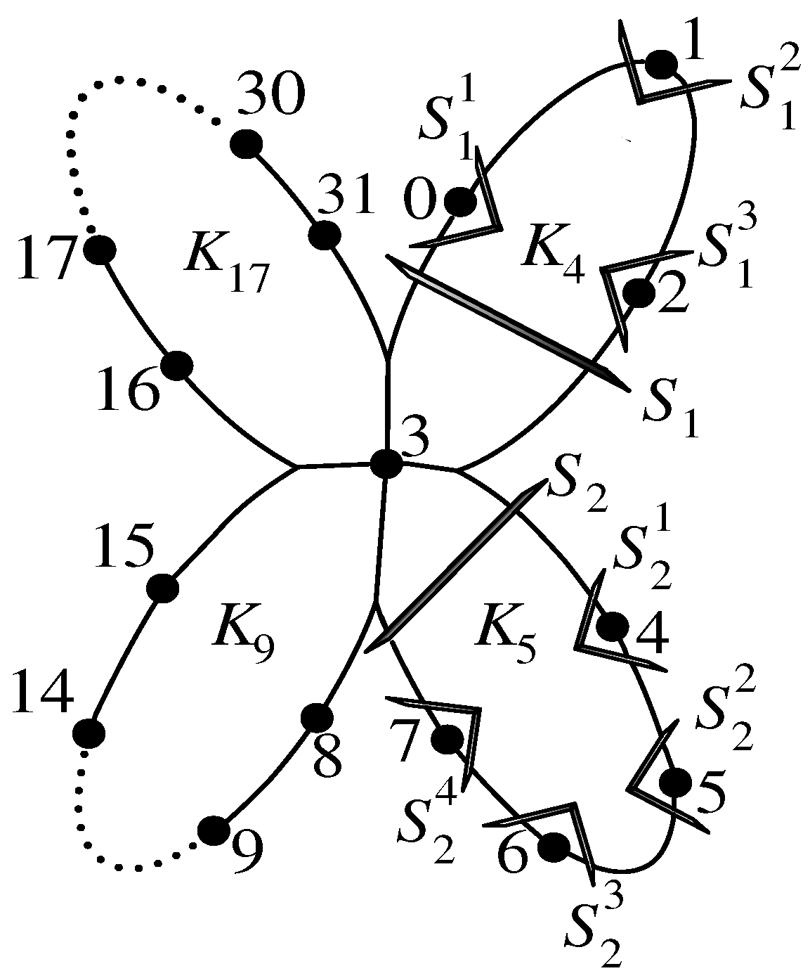
Definition 2. [11] Let be a complete graph on vertices, . Let and for all such that has one vertex as common. The resultant graph is called a windmill graph and is denoted by . Remark 2. We denote = , and . Then the windmill graph has vertices, see Figure 1. Theorem 2. The wirelength of into is given by
Proof. The proof is divided into three parts A, B, and C comprising of the embedding algorithm, proof of correctness, and computation of wirelength, respectively.
Part A:
Label the vertices of by lexicographic order from 0 to . Label the vertices of in as such that is the label of common vertex s. For , label the vertices of (except s) in as . Define an embedding f of into given by .
Part B:
We assume that the labels represent the vertices to which they are assigned.
Table 1 gives the notations for edge cuts of windmill graph as depicted in
Figure 1.
Then {: } ∪ { :, } is a partition of . The edge cut of disconnects into two components and where . Let and be the preimage of and under f respectively. By Lemmas 4 & 5, is an optimal set and each satisfies conditions (i)–(iii) of the Congestion Lemma. Therefore, is minimum.
Similarly, the edge cut of disconnects into two components and where . Let and be the preimage of and under f respectively. Since is an optimal set and each satisfies conditions of the Congestion Lemma. Therefore, is minimum. The 2-Partition Lemma implies that = .
Part C:
By Part B, we have , for all , . Therefore, the wirelength of enhanced hypercube into windmill graph is given by = = □
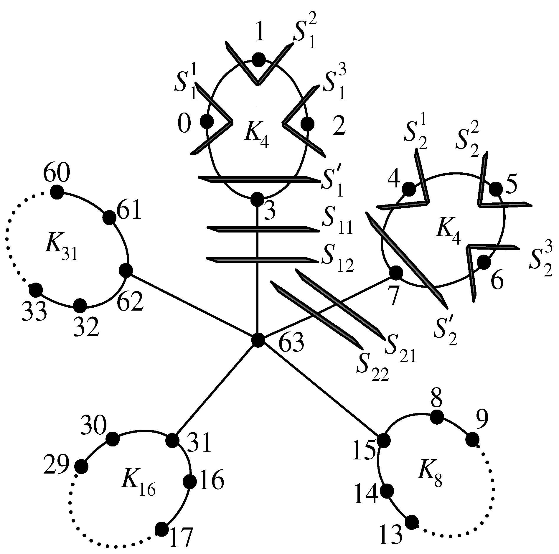
Definition 3 ([
11]).
Let be a star graph on vertices (say ) and be complete graphs on vertices, . Let , for all and such that has as common. The resultant graph is called a complete star necklace and is denoted by . Remark 3. We denote = , where . Then the complete star necklace has vertices, see Figure 2. Theorem 3.
Proof. The proof technique is similar to Theorem 2 as divided into three parts A, B, and C.
Part A:
Label the vertices of by lexicographic order from 0 to . For , label the vertices of in as such that is the label of , and as . Define an embedding f of into given by .
Part B:
We assume that the labels represent the vertices to which they are assigned.
Table 2 gives the notations for edge cuts of complete star necklace graph as depicted in
Figure 2.
Then {, , : } ∪ {:, } is a partition of . The edge cut of disconnects into two components and where . Let and be the preimage of and under f respectively. By Lemma 4, is an optimal set and each satisfies conditions (i)–(iii) of the Congestion Lemma. Therefore, is minimum. Similarly, is minimum.
The edge cut of disconnects into two components and where . Let and be the preimage of and under f respectively. By Lemma 5, is an optimal set and each satisfies conditions (i)–(iii) of the Congestion Lemma. Therefore, is minimum.
The edge cut of disconnects into two components and where . Let and be the preimage of and under f respectively. Since is an optimal set and each satisfies conditions of the Congestion Lemma. Therefore, is minimum. The 2-Partition Lemma implies that .
Part C:
By Part B, we have , , for all , . Therefore, the wirelength of enhanced hypercube into complete star necklace graph is given by . □
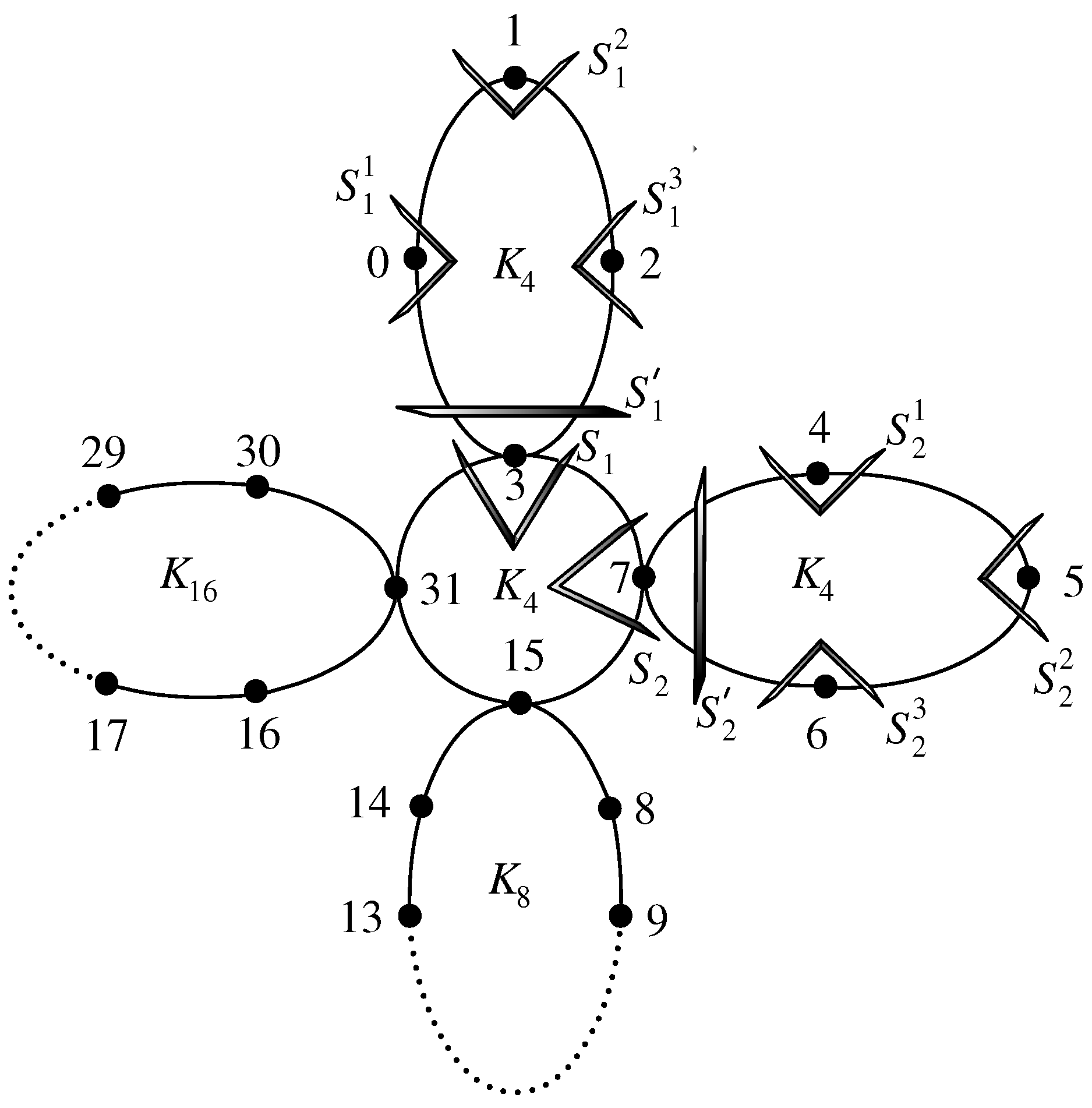
Definition 4 ([
11]).
Let be a complete graph on m vertices (say ) and be complete graphs on vertices, . Let and for all such that has as common. The resultant graph is called a circular necklace graph and is denoted by . Remark 4. We denote = , where . Then the circular necklace has vertices, see Figure 3. Theorem 4. The wirelength of into is given by
Proof. We label the vertices of by lexicographic order from 0 to . For , label the vertices of in as such that is the label of . Define an embedding f of into given by .
We assume that the labels represent the vertices to which they are assigned.
Table 3 gives the notations for edge cuts of circular necklace graph as depicted in
Figure 3.
Then { , : } ∪ { :, } is a partition of . The edge cut of disconnects into two components and where . Let and be the preimage of and under f respectively. By Lemma 4, is an optimal set and each satisfies conditions of the Congestion Lemma. Therefore, is minimum.
The edge cut of disconnects into two components and where . Let and be the preimage of and under f respectively. By Lemma 5, is an optimal set and each satisfies conditions (i)–(iii) of the Congestion Lemma. Therefore, is minimum.
The edge cut of disconnects into two components and where . Let and be the preimage of and under f respectively. Since is an optimal set and each satisfies conditions (i)–(iii) of the Congestion Lemma. Therefore is minimum. The 2-Partition Lemma implies that .
Now, we have , , for all , . Therefore, the wirelength of enhanced hypercube into circular necklace graph is given by = = □


