Abstract
The number of subtrees, or simply the subtree number, is one of the most studied counting-based graph invariants that has applications in many interdisciplinary fields such as phylogenetic reconstruction. Motivated from the study of graph surgeries on evolutionary dynamics, we consider the subtree problems of fan graphs, wheel graphs, and the class of graphs obtained from “partitioning” wheel graphs under dynamic evolution. The enumeration of these subtree numbers is done through the so-called subtree generation functions of graphs. With the enumerative result, we briefly explore the extremal problems in the corresponding class of graphs. Some interesting observations on the behavior of the subtree number are also presented.
1. Introduction
The study of graph invariants or topological indices has been proven to be of crucial importance in various interdisciplinary topics. Generally, the existing known topological indices could be divided into distance-based, degree-based, or structure-based ones; some of the studies on these three categories are referred to in [1,2,3,4] and the references therein. The number of subtrees, or simply the subtree number, is one of the counting-based graph invariants.
Finding and/or enumerating special topological structures or graph patterns has become an important problem due to their applications including, to name a few, frequent subgraphs mining [5], network optimization design [6,7], and local network reliability [8,9]. In particular, the subtree number has also been shown to be correlated to phylogenetic reconstruction [10] and various chemical indices such as the Wiener index (closely correlated with the boiling point of paraffin [3]), the Merrifield–Simmons index, and the Hosoya index [11]. Research results also show that there exists an amazing “negative correlation” between the number of subtrees and the Wiener index [12,13,14,15,16,17]. Therefore, the subtree number index can indirectly characterize the physical–chemical characteristics of molecules.
Various topics related to the subtree number have been explored over the past years, such as extremal problems [12,18,19], the subtree density problem [20,21,22], generic chemical structures storage problems [23,24], fault tolerant computing and parallel scheduling [25,26], recognition of substructure [27], simplification of the flow networks [28], Markovian queuing systems decomposition [29], and matching problems [30,31].
By using “generating functions”, Yan and Yeh [4] presented a linear-time algorithm to evaluate the subtree weight sum of a tree, leading to an algorithmic approach to compute the subtree number of a tree. Following this approach and more recently, Yang et al. [32,33] proposed enumerating algorithms for BC-subtrees of trees, unicyclic, and edge-disjoint bicyclic graphs and computed the subtree number on spiro and polyphenyl hexagonal chains [17]. With structure mapping and weights transferring of cycles, Yang et al. [34] also presented enumerating algorithms for subtrees of hexagonal and phenylene chains. More recently, Chin et al. [35] presented the subtree number of complete graphs, complete bipartite graphs, and theta graphs, as well as the ratio of spanning trees to all subtrees of the above graphs.
Let be a weighted star on vertices with center , vertex weight function for all , and edge weight function for all . Suppose the n leaves are labeled, in counterclockwise order, , then the wheel graph is obtained from by adding the edges for (here we let ).
As is well known, star and wheel graphs are very typical network topologies used in designing and implementing communication networks. The wheel graph is the planar graph with a chromatic number not greater than 4. Specifically, the chromatic number of is 3 for odd n and 4 for even n. Some researchers have tried to apply this property of to prove the famous Four Color Theorem [36]. Moreover, can also be used in wireless ad hoc networks [37]. Therefore, it is worth studying the new structural characteristics of these two graphs, especially from new perspectives.
Inspired by the significant effect of graph surgeries on evolutionary dynamics in [38], we are motivated to study the subtree number in graphs resulting from graph surgeries. In particular, we will consider a class of graphs that “lie in between” the fan and wheel graphs, called the “partitions” (explanation will be given later) of wheel graphs.
Definition 1.
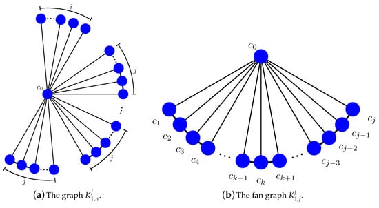
Given the star on vertices defined above with center vertex and , the graph is obtained from by adding the edges for all except for (see Figure 1a). If , we call the fan graph on vertices. It is also easy to see that is the single vertex , and is the star .
Figure 1.
The graph and the fan graph .
From the definitions of the graph and the wheel graph , we see that the graph can be vividly described in terms of through “partitions” (and deletion of edges ) perspective.
The reason that we consider our graphs as vertex and edge weighted is to use the so-called subtree generating functions. We assume a graph to be a weighted graph and define the vertex-weight function and edge-weight function , where ℜ is the real number. Unless otherwise noted, for a graph G, we initialize its vertex weight function for each and its edge weight function for each throughout this paper.
The following notations need to be listed before introducing the main tool:
- denotes the graph obtained from G by removing all elements of X;
- (resp. ) denotes the set of subtrees of G (resp. containing v);
- denotes the set of subtrees of G containing the edge ;
- denotes the weight of subtree ;
- is the sum of weights of subtrees in ;
- is the cardinality (namely the number) of the corresponding set of subtrees.
We define the weight of a subtree of G, denoted by , as the product of the weights of the vertices and edges in . The generating function of subtrees of G, denoted by , is the sum of weights of subtrees of G. Namely, . Similarly, we define
By substituting each vertex weight and edge weight in these generating functions, we have the corresponding numbers of subtrees under various constraints, i.e., and .
We introduce the following lemma, which will frequently be used in our work.
Lemma 1.
[4] Let be a path on n vertices, with vertex weight function for all and edge weight function for all , then .
In Section 2, we will present the subtree generating functions of and the wheel graph . Through using these generating functions and theoretical analysis, we study the extremal graphs, subtree fitting problems, and subtree density behaviors of these graphs in Section 3. Lastly, in Section 4, we summarize our results and comment on potential topics for future work.
2. Subtree Generating Functions of and Wheel Graph
In this section, we will establish the subtree generating functions of and wheel graph and provide the theoretical background for our computational analysis. We start by studying the subtree problem of .
2.1. Subtree Generating Functions and Subtree Numbers of
Theorem 1.
Let be the weighted graph defined as above, and be non-negative integers with and . Then
with , and , .
Proof.
We consider the subtrees of by cases
- (i)
- not containing the center ,
- (ii)
- containing the center .
From Lemma 1, we have the subtree generating function of case (i) as
With the contraction method of [4] and structure analysis, we have the subtree generating function of case (ii) as
Denote and , and divide all subtrees for (see Figure 1b) into four cases where
- is the collection of subtrees that contain neither nor ;
- is the collection of subtrees that contain , but not ;
- is the collection of subtrees that contain , but not ;
- is the collection of subtrees that contain both and .
From the definitions of subtree weight and subtree generating function, we know that:
(a) ;
(b) , where are the trees obtained from by attaching an edge at vertex ;
(c) We can write as
for and ;
(d) For each subtree , we know that must not contain the edge . Consequently, we can further consider the subtrees that contain edges but not recursively for .
With (a)–(d),we have
Following similar arguments to Theorem 1, we can also obtain the subtree generating functions of the graphs obtained from identifying the centers of different fan graphs (). We skip the tedious details for the sake of space.
Theorem 2.
Let be different weighted fan graphs, and suppose there are copies of for . Let be the graph that is constructed by identifying the centers of these fan graphs with . Then
with and , .
Actually, a single fan graph is a special case of the above discussion, so we can further obtain the subtree generating function for the subtrees containing a particular vertex. Again, we skip the similar but technical details.
Theorem 3.
Adding an edge between any two fan graphs (to construct a bigger fan) of a graph will also increase the number of subtrees. Let G be the weighted graph as defined in Theorem 2, and suppose (with non-center vertices labeled counterclockwise as ) and (with non-center vertices labelled clockwise as ) are the two sub-fan graphs of G with . Define to be the graph obtained from G by adding one edge . Meanwhile, denote the graph of that contains , and denote the collection of subtrees in that contain . By dividing the subtrees of G and into two cases of containing center or not, with Lemma 1, definitions of subtree weight and subtree generating function, and combining structure analysis, we have the following theorem:
Theorem 4.
Let G and be the weighted graphs defined above. Then,
By letting in the subtree generating functions from the above theorems, we have the corresponding subtree numbers of the various related graphs above.
Corollary 1.
The subtree number of is
with .
With Corollary 1, we have the number of subtrees of that contain central vertex as illustrated in Figure 2.
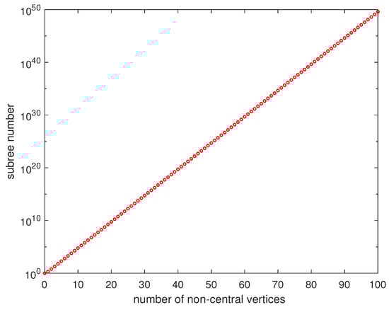
Figure 2.
Number of subtrees of that contain central vertex , in semi-log(Log-Y) coordinates.
Corollary 2.
Let be positive integers with , and , then
with and .
With Corollary 2, we have the subtree number of , see details in Section 3.1.
Corollary 3.
Let , , and l be defined in Theorem 2, then
with and , .
Let be the graph defined in Theorem 2 with ; ; ; , with Corollary 1 and Corollary 3, we have .
Corollary 4.
The number of subtrees of the fan graph containing is
with and , .
Similarly, the number of subtrees of that contain central vertex (see Figure 3) can be obtained from Corollary 4.
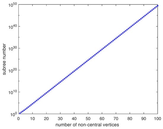
Figure 3.
Number of subtrees of that contain the vertex , in semi-log(Log-Y) coordinates.
Corollary 5.
Let G be the graph defined in Theorem 2, and be a merged graph from G with and (Theorem 4), then
where is the number of subtrees containing both vertex and edge .
Let G, , and be the graphs defined in Corollary 5 with ; , and , with Corollary 1, Corollary 5, and structural analysis, we have = 77,997, , and = 129,303.
2.2. Subtree Generating Function and Subtree Number of Wheel Graph
Next we consider the subtree generating function of the weighted wheel graph .
Theorem 5.
Let be the weighted wheel graph on vertices with vertex weight function and edge weight function . Then
with , , , and .
Proof.
For convenience, we let for , and for . We also follow the convention that if , and , if .
We first consider the subtrees of in different cases:
(i) not containing the edge ,
(ii) containing the edge .
The subtrees in case (i) can be further partitioned into four categories. As a result, we have
where
- is the set of subtrees of that contain neither nor ;
- is the set of subtrees of that contain , but not ;
- is the set of subtrees of that contain but not ;
- is the set of subtrees of that contain both and .
From the definition of subtree weight and with structure analysis, we have
and
Thus, we have
Similarly, for case (ii), we have
where
- is the set of subtrees in that contain neither nor ;
- is the set of subtrees in that contain , but not ;
- is the set of subtrees in that contain but not ;
- is the set of subtrees in that contain both and .
Analyzing each case, we have:
(a) , where are the trees obtained from by attaching the edge at vertex ;
(b) , where is the graph of that contains , and obviously, ;
(c) for ;
(d) In a similar manner as (b) and (c), use variables l and r to count the number of edges trailing off and , respectively, then the subtrees in are indexed by these two variables, which count extra edges that are on the two sides of the T shape containing the 3 edges required by . With (a)–(d), we have
Now with Equations (23)–(25), we have
By Theorem 1, Theorem 3, and Equations (22) and (26), we have
Letting in Equation (18), we have the following corollary.
Corollary 6.
The subtree number of is
with , , and .
With Corollary 6, the subtree numbers of are shown in Table 1.

Table 1.
The subtree numbers of wheel graph ().
As a matter of fact, with the generating function and further structural and theoretical analysis, we can also solve the subtree generation computing problems for the following more generalized types of graphs; here we skip the similar but technical details.
(i) Graph is constructed by identifying the center of l graphs to , where is the graph constructed from a vertex and a path by connecting with , , and any other arbitrary vertices on the path ; for the special case , the graph is a path on vertices and .
(ii) Graph , namely the graph obtained from wheel by deleting random l different edges (each is different the others).
3. Behaviors of and in Terms of Subtrees
With the subtree generating functions established, we can now analyze the behaviors of the graphs and in terms their subtree numbers and other related properties.
3.1. Subtree Numbers and
We start with the subtree numbers of the graphs for different n and j. First, we take a quick look at the extremal problems.
Proposition 1.
Among all :
- the graph has subtrees, fewer than any other ; and
- the graph has subtrees (where and ), more than any other .
Proof.
Note that adding an edge to a graph will strictly increase the subtree number. The extremal structures and then follow immediately from the fact that the former is a subgraph of any and the latter contains any as a subgraph. □
We are also interested in knowing which () has the second- or third-largest subtree number. To examine this, we also explore how the subtree numbers of the graphs behave. With Corollary 2 and Matlab computing (see Appendix A for more details), we obtain the subtree number behaviors of as shown in Figure 4.
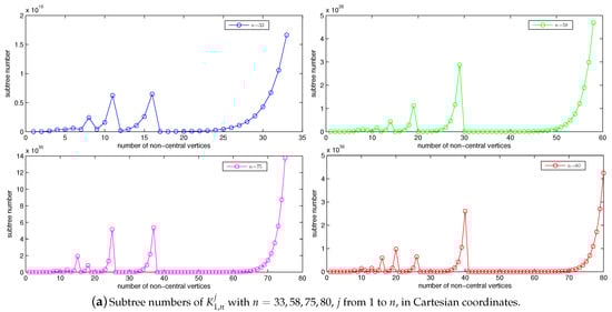
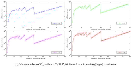
Figure 4.
Subtree numbers of with , j from 1 to n, in semi-log(Log-Y) coordinates.
It seems from Figure 4a,b that among all :
- has the second-largest subtree number; and
- has the third-largest subtree number for odd (or sufficiently large) n.
- the subtree number increment trend meets exponential growth when .
In general, it is not difficult to show the following.
Proposition 2.
Suppose (i.e., n is much larger than k), then among all , the graph has the -th largest subtree number.
The proof follows from adjusting the “sizes” of the two sub-fan graphs of . We skip the details here. The same argument can also show the monotonic behavior for large enough j.
Proposition 3.
If , then has a larger subtree number than .
Understanding the specific behavior of for general j in terms of the subtree number seems to be an interesting and nontrivial problem.
Similarly, from Corollary 6, we can obtain the subtree numbers of wheel graph , as already shown in Table 1. On the other hand, experimental observation shows that the subtree numbers of increase very fast and this growth trend seems to fit the linear regression model after doing the logarithmic transformation. Through implementing the linear regression in the MATLAB software for data of the number of subtrees of from to 602, the appropriate formula for the subtree number of can be stated as
As , Equation (31) can be rewritten as
With Corollary 6, Equation (32), and logarithmic transformation for each subtree number of and fitted value, we can obtain the subtree number trend of , as illustrated in Figure 5 where the original and fitted data are respectively marked in red and blue. We believe Equation (32) can be proved or disproved through traditional analytic combinatorial approaches, but we will not pursue the technical analysis here.
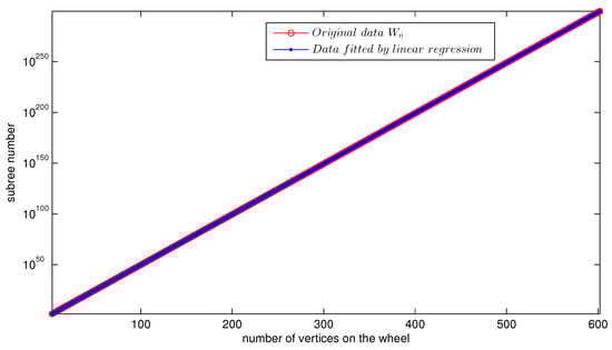
Figure 5.
Subtree number trend of wheel graph , in semi-log(Log-Y) coordinates.
Our work can also be easily applied to more general “partitions” of wheel graphs instead of just the s. To illustrate the observations, we introduce some simple notations. Given a positive integer n and partition of n (with and ), the graph is obtained from by adding edges for all except for , for . It seems that the subtree numbers of s coincide with some sort of ordering of the partitions π of n. In general, larger and fewer parts in π results in more subtrees in . More precise statements along this line requires further study.
3.2. Subtree Densities of and
The subtree generating function can be used to provide more information than just the number of subtrees. For instance, using the subtree generating function, one can easily obtain the total number of vertices in all subtrees, from which we have the average subtree order in a given graph. The ratio of the average subtree order and the order of the original graph is called the subtree density of the graph. We present the formal subtree density definition as follows:
Definition 2
([20]). Suppose G is a graph with n vertices, then is the average order of the subtrees of G, where are the orders of all of G’s k non-empty subtrees, and the subtree density of G is defined as .
It is essentially the probability that a vertex chosen at random from G will belong to a randomly chosen subtree of G. Some of the work related to subtree densities can be found in [20,21,39].
With Theorem 1, Theorem 5, and substituting , we could obtain the vertex generating function of subtrees of and , respectively, i.e., and ). The subtree density of and is simply
where denotes the vertex number of , and can be or .
We will now apply this to find the subtree densities of and .
Clearly, the vertex number of and is , namely
With Theorem 1 and letting in Equation (1), we obtain the vertex generating function of subtrees of .
with , and , .
Similarly, letting in Equation (18), we obtain the vertex generating function of subtrees of .
with , and , .
From Equations (33)–(35), we can obtain the subtree densities of (plotted in Figure 6); related data can be found in Table 2. Similarly, from Equations (33), (34), and (36), we have subtree densities plotted in Figure 7; related data are listed in Table 3.
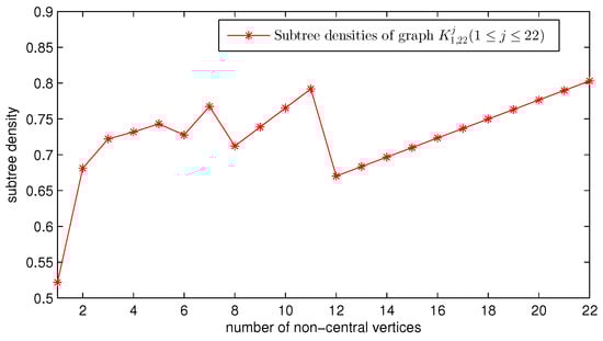
Figure 6.
Subtree densities of the graphs .
Table 2.
Related data for , with and .
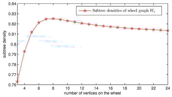
Figure 7.
Subtree densities of wheel graph .
Table 3.
Related data for wheel graph .
From Table 2 and Figure 6, it appears that and have the smallest and second-smallest subtree densities, respectively. grows linearly with the increase of j. Moreover, from Table 3 and Figure 7, we see that increases first in the interval and reaches the maximum value when , and then decreases gradually in the interval and approximates the limit value of .
Similarly, as studied in paper [35], we can also discuss the ratio of spanning trees to all subtrees and spanning tree densities of and . We skip the details here.
4. Concluding Remarks
In this paper we established the subtree generating functions of the wheel graph and “partitions” , along with other related structures such as the fan graphs. With the subtree generating functions, we are able to study the subtree number and subtree densities of these graphs. From our computational analysis, several theoretical conclusions are drawn, especially on the extremal problems with respect to the subtree number. These results provide a fundamental basis for studying subtree problems of multi-cyclic graphs, chemical compounds, and complex graphs.
As one can see, the computational results in Section 3.2 show interesting observations on the characteristics of these structures. Attempting to verify some of them, especially on those related to the subtree densities, and exploring the BC-subtree number index, Wiener index, Harary index, atom-bond connectivity trends of wheel graph , “partitions” , and their generalizations would make very interesting projects for future work. Exploring the novel structural properties from the evolutionary perspective of graphs with more complicated cycle structures, particularly some important nanomaterials such as the pentagonal carbon nanocone, is also a very attractive future topic.
Author Contributions
H.W, Y.Y and A.W contributed to supervision, project administration, and the formal analysis. W.-T.Z and D.-Q.S contributed to the methodology and writing of the original draft preparation. The final draft was written by H.W and Y.Y.
Funding
This work is supported by the National Natural Science Foundation of China (grant nos. 61702291, 61772102, 61472058,11531001), the China Postdoctoral Science Foundation (grant no. 2018M632095), the Program for Science & Technology Innovation Talents in Universities of Henan Province (grant no. 19HASTIT029), the Joint NSFC-ISF Research Program (jointly funded by the National Natural Science Foundation of China and the Israel Science Foundation (No. 11561141001)), the Key Research Project in Universities of Henan Province (grant nos. 19B110011, 19B630015), the Scientific Research Starting Foundation for High-Level Talents of Pingdingshan University (grant no.PXY-BSQD2017006), and the Simons Foundation (grant no. 245307).
Conflicts of Interest
The authors declare no conflict of interest.
Appendix A. Matlab Code, Python Code, And Data
In what follows, we provide the source codes related to Figure 4. Python code Pythoncode1 (derived from Corollary 2) can output the data files “n=33.txt”, “n=58.txt”, “n=75.txt”, and “n=80.txt” by inputting the integer 33, 58, 75, 80, respectively. MATLAB codes MCF1a, MCF1b can draw the Figure 4a,b, respectively.
| Pythoncode1. The Python code for computing the subtree number of . | |
| 1 | n=int (input()) |
| 2 | b=[−1 for i in range (n+1)] |
| 3 | b[0]=1 |
| 4 | b[1]=2 |
| 5 | for j in range (1,n+1): |
| 6 | sum1=0 |
| 7 | for r in range (1,j+1): |
| 8 | sum1=sum1+r∗b[j−r] |
| 9 | b[j]=b[j−1]+sum1 |
| 10 | file_name="n="+str(n)+".txt" |
| 11 | file = open (file_name,’w’) |
| 12 | for j in range (1,n+1): |
| 13 | i = n%j |
| 14 | s=(j+1)∗(n−i)/2+i+2∗∗(i)∗b[j]∗∗((n−i)/j) |
| 15 | file.write (str(s)) |
| 16 | file.write (’\n’) |
| 17 | print (s) |
| MCF1a. MATLAB source code for Figure 1a. | |
| 1 | clear; |
| 2 | clc; |
| 3 | s1 = load(’n=33.txt’); |
| 4 | s2 = load(’n=58.txt’); |
| 5 | s3 = load(’n=75.txt’); |
| 6 | s4 = load(’n=80.txt’); |
| 7 | format long; |
| 8 | A =cell(1,10); |
| 9 | A{1,1}=’−bo’; |
| 10 | A{1,2}=’−go’; |
| 11 | A{1,3}=’−mo’; |
| 12 | A{1,4}=’−ro’; |
| 13 | subplot(2,2,1); |
| 14 | plot(s1,A{1,1}); |
| 15 | axis normal; |
| 16 | set(legend(’n=33’),’fontsize’,8); |
| 17 | xlabel(’number of non-central vertices’); |
| 18 | ylabel(’subtree number’); |
| 19 | subplot(2,2,2); |
| 20 | plot(s2,A{1,2}); |
| 21 | set(legend(’n=58’),’fontsize’,8); |
| 22 | xlabel(’number of non-central vertices’); |
| 23 | ylabel(’subtree number’); |
| 24 | subplot(2,2,3); |
| 25 | plot(s3,A{1,3}); |
| 26 | axis normal; |
| 27 | set(legend(’n=75’),’fontsize’,8); |
| 28 | xlabel(’number of non-central vertices’); |
| 29 | ylabel(’subtree number’); |
| 30 | subplot(2,2,4); |
| 31 | plot(s4,A{1,4}); |
| 32 | set(legend(’n=80’),’fontsize’,8); |
| 33 | xlabel(’number of non-central vertices’); |
| 34 | ylabel(’subtree number’); |
| MCF1b: The MATLAB source code for Figure 1b. | |
| 1 | clear; |
| 2 | clc; |
| 3 | s1 = load(’n=33.txt’); |
| 4 | s2 = load(’n=58.txt’); |
| 5 | s3 = load(’n=75.txt’); |
| 6 | s4 = load(’n=80.txt’); |
| 7 | format long; |
| 8 | A =cell(1,10); |
| 9 | A{1,1}=’−bo’; |
| 10 | A{1,2}=’−go’; |
| 11 | A{1,3}=’−mo’; |
| 12 | A{1,4}=’−ro’; |
| 13 | subplot(2,2,1); |
| 14 | semilogy(s1,A{1,1}); |
| 15 | axis normal; |
| 16 | set(legend(’n=33’,’location’,’southeast’),’fontsize’,8); |
| 17 | xlabel(’number of non-central vertices’); |
| 18 | ylabel(’subtree number’); |
| 19 | subplot(2,2,2); |
| 20 | semilogy(s2,A{1,2}); |
| 21 | set(legend(’n=58’,’location’,’southeast’),’fontsize’,8); |
| 22 | xlabel(’number of non-central vertices’); |
| 23 | ylabel(’subtree number’); |
| 24 | subplot(2,2,3); |
| 25 | semilogy(s3,A{1,3}); |
| 26 | axis normal; |
| 27 | set(legend(’n=75’,’location’,’southeast’),’fontsize’,8); |
| 28 | xlabel(’number of non-central vertices’); |
| 29 | ylabel(’subtree number’); |
| 30 | subplot(2,2,4); |
| 31 | semilogy(s4,A{1,4}); |
| 32 | set(legend(’n=80’,’location’,’southeast’),’fontsize’,8); |
| 33 | xlabel(’number of non-central vertices’); |
| 34 | ylabel(’subtree number’); |
References
- Das, K.C. Atom-bond connectivity index of graphs. Discret. Appl. Math. 2010, 158, 1181–1188. [Google Scholar] [CrossRef]
- Dobrynin, A.A.; Entringer, R.; Gutman, I. Wiener index of trees: Theory and applications. Acta Appl. Math. 2001, 66, 211–249. [Google Scholar] [CrossRef]
- Wiener, H. Structural determination of paraffin boiling points. J. Am. Chem. Soc. 1947, 1, 17–20. [Google Scholar] [CrossRef]
- Yan, W.; Yeh, Y. Enumeration of subtrees of trees. Theor. Comput. Sci. 2006, 369, 256–268. [Google Scholar] [CrossRef]
- Ingalalli, V.; Ienco, D.; Poncelet, P. Mining frequent subgraphs in multigraphs. Inf. Sci. 2018, 451, 50–66. [Google Scholar] [CrossRef]
- Tilk, C.; Irnich, S. Combined column-and-row-generation for the optimal communication spanning tree problem. Comput. Oper. Res. 2018, 93, 113–122. [Google Scholar] [CrossRef]
- Zetina, C.A.; Contreras, I.; Fernández, E.; Luna-Mota, C. Solving the optimum communication spanning tree problem. Eur. J. Oper. Res. 2019, 273, 108–117. [Google Scholar] [CrossRef]
- Chechik, S.; Emek, Y.; Patt-Shamir, B.; Peleg, D. Sparse reliable graph backbones. Inf. Comput. 2012, 210, 31–39. [Google Scholar] [CrossRef][Green Version]
- Xiao, Y.; Zhao, H.; Liu, Z.; Mao, Y. Trees with large numbers of subtrees. Int. J. Comput. Math. 2017, 94, 372–385. [Google Scholar] [CrossRef]
- Knudsen, B. Optimal multiple parsimony alignment with affine gap cost using a phylogenetic tree. Algorithms Bioinform. Lect. Notes Comput. Sci. 2003, 2812, 433–446. [Google Scholar]
- Wagner, S.G. Correlation of graph-theoretical indices. SIAM J. Discret. Math. 2007, 21, 33–46. [Google Scholar] [CrossRef]
- Székely, L.; Wang, H. On subtrees of trees. Adv. Appl. Math. 2005, 34, 138–155. [Google Scholar]
- Székely, L.; Wang, H. Binary trees with the largest number of subtrees. Discret. Appl. Math. 2007, 155, 374–385. [Google Scholar]
- Zhang, X.; Zhang, X.; Gray, D.; Wang, H. The number of subtrees of trees with given degree sequence. J. Graph Theory 2013, 73, 280–295. [Google Scholar] [CrossRef]
- Wang, H. The extremal values of the Wiener index of a tree with given degree sequence. Discret. Appl. Math. 2008, 156, 2647–2654. [Google Scholar] [CrossRef]
- Deng, H. Wiener indices of spiro and polyphenyl hexagonal chains. Math. Comput. Model. 2012, 55, 634–644. [Google Scholar] [CrossRef]
- Yang, Y.; Liu, H.; Wang, H.; Fu, H. Subtrees of spiro and polyphenyl hexagonal chains. Appl. Math. Comput. 2015, 268, 547–560. [Google Scholar] [CrossRef]
- Czabarka, É.; Székely, L.A.; Wagner, S. On the number of nonisomorphic subtrees of a tree. J. Graph Theory 2018, 87, 89–95. [Google Scholar] [CrossRef]
- Zhang, X.; Zhang, X. The Minimal Number of Subtrees with a Given Degree Sequence. Graphs Comb. 2015, 31, 309–318. [Google Scholar] [CrossRef]
- Jamison, R.E. On the average number of nodes in a subtree of a tree. J. Comb. Theory Ser. B 1983, 35, 207–223. [Google Scholar] [CrossRef]
- Vince, A.; Wang, H. The average order of a subtree of a tree. J. Comb. Theory Ser. B 2010, 100, 161–170. [Google Scholar] [CrossRef]
- Wagner, S.; Wang, H. On the Local and Global Means of Subtree Orders. J. Graph Theory 2016, 81, 154–166. [Google Scholar] [CrossRef]
- Nakayama, T.; Fujiwara, Y. BCT Representation of Chemical Structures. J. Chem. Inf. Comput. Sci. 1980, 20, 23–28. [Google Scholar] [CrossRef]
- Nakayama, T.; Fujiwara, Y. Computer representation of generic chemical structures by an extended block-cutpoint tree. J. Chem. Inf. Comput. Sci. 1983, 23, 80–87. [Google Scholar] [CrossRef]
- Frederickson, G.N.; Hambrusch, S.E. Planar linear arrangements of outerplanar graphs. IEEE Trans. Circuits Syst. 1988, 35, 323–333. [Google Scholar] [CrossRef]
- Wada, K.; Luo, Y.; Kawaguchi, K. Optimal fault-tolerant routings for connected graphs. Inf. Process. Lett. 1992, 41, 169–174. [Google Scholar] [CrossRef]
- Heath, L.; Pemmaraju, S. Stack and queue layouts of directed acyclic graphs: Part II. SIAM J. Comput. 1999, 28, 1588–1626. [Google Scholar] [CrossRef]
- Misiolek, E.; Chen, D.Z. Two flow network simplification algorithms. Inf. Process. Lett. 2006, 97, 197–202. [Google Scholar] [CrossRef]
- Fox, D. Block cutpoint decomposition for markovian queueing systems. Appl. Stoch. Model. Data Anal. 1988, 4, 101–114. [Google Scholar] [CrossRef]
- Barefoot, C. Block-cutvertex trees and block-cutvertex partitions. Discret. Math. 2002, 256, 35–54. [Google Scholar] [CrossRef][Green Version]
- Mkrtchyan, V. On trees with a maximum proper partial 0-1 coloring containing a maximum matching. Discret. Math. 2006, 306, 456–459. [Google Scholar] [CrossRef]
- Yang, Y.; Liu, H.; Wang, H.; Feng, S. On algorithms for enumerating BC-subtrees of unicyclic and edge-disjoint bicyclic graphs. Discret. Appl. Math. 2016, 203, 184–203. [Google Scholar] [CrossRef]
- Yang, Y.; Liu, H.; Wang, H.; Makeig, S. Enumeration of BC-subtrees of trees. Theor. Comput. Sci. 2015, 580, 59–74. [Google Scholar] [CrossRef]
- Yang, Y.; Liu, H.; Wang, H.; Deng, A.; Magnant, C. On Algorithms for Enumerating Subtrees of Hexagonal and Phenylene Chains. Comput. J. 2017, 60, 690–710. [Google Scholar] [CrossRef]
- Chin, A.J.; Gordon, G.; MacPhee, K.J.; Vincent, C. Subtrees of graphs. J. Graph Theory 2018, 89, 413–438. [Google Scholar] [CrossRef]
- Cahit, I. Spiral chains: A new proof of the four color theorem. arXiv 2004, arXiv:0408247. [Google Scholar]
- Yang, Z.; Liu, Y.; Li, X.Y. Beyond trilateration: On the localizability of wireless ad hoc networks. IEEE/ACM Trans. Netw. (ToN) 2010, 18, 1806–1814. [Google Scholar] [CrossRef]
- Allen, B.; Lippner, G.; Chen, Y.T.; Fotouhi, B.; Momeni, N.; Yau, S.T.; Nowak, M.A. Evolutionary dynamics on any population structure. Nature 2017, 544, 227. [Google Scholar] [CrossRef]
- Haslegrave, J. Extremal results on average subtree density of series-reduced trees. J. Comb. Theory Ser. B 2014, 107, 26–41. [Google Scholar] [CrossRef]
© 2019 by the authors. Licensee MDPI, Basel, Switzerland. This article is an open access article distributed under the terms and conditions of the Creative Commons Attribution (CC BY) license (http://creativecommons.org/licenses/by/4.0/).