Abstract
In this paper, a novel improved whale optimization algorithm (IWOA), based on the integrated approach, is presented for solving the flexible job shop scheduling problem (FJSP) with the objective of minimizing makespan. First of all, to make the whale optimization algorithm (WOA) adaptive to the FJSP, the conversion method between the whale individual position vector and the scheduling solution is firstly proposed. Secondly, a resultful initialization scheme with certain quality is obtained using chaotic reverse learning (CRL) strategies. Thirdly, a nonlinear convergence factor (NFC) and an adaptive weight (AW) are introduced to balance the abilities of exploitation and exploration of the algorithm. Furthermore, a variable neighborhood search (VNS) operation is performed on the current optimal individual to enhance the accuracy and effectiveness of the local exploration. Experimental results on various benchmark instances show that the proposed IWOA can obtain competitive results compared to the existing algorithms in a short time.
1. Introduction
In recent years, scheduling played a crucial role in almost all manufacturing systems, as global competition became more and more intense. The classical job shop scheduling problem (JSP) is one of the most important scheduling forms existing in real manufacturing. It became a hotspot in the academic circle and received a large amount of attention in the research literature with its wide applicability and inherent complexity [1,2,3]. In JSP, a group of jobs need to be processed on a set of machines, where each job consists of a set of operations with a fixed order. The processing of each operation of the jobs must be performed on a given machine. Each machine is continuously available at time zero and can process only one operation at a time without interruption. The decision concerns how to sequence the operations of all the jobs on the machines, so that a given performance indicator can be optimized. Makespan is the time in which all the jobs need to be completed and is a typical performance indicator for the JSP.
The flexible job shop scheduling problem (FJSP) is an extension of the classical JSP, where each operation can be processed by any machine in a given set rather than one specified machine. The FJSP is closer to a real manufacturing environment compared with classical JSP. According to its practical applicability, the FJSP became very crucial in both academic and application fields. However, it is more difficult than classical JSP because it contains an additional decision problem, assigning operations to the appropriate machine. Therefore, the FJSP is a problem of challenging complexity and was proven to be non-deterministic polynomial-time (NP)-hard [4].
In the initial study, Brucker and Schlie firstly proposed a polynomial algorithm for solving the FJSP with two jobs [5]. During the past two decades, the FJSP attracted the interest of many researchers. There were many approximation algorithms, mainly metaheuristics, presented for solving the FJSP. Dauzere-Peres and Paulli [6] proposed a tabu search (TS) algorithm which was based on a new neighborhood structure for the FJSP. Mastrolilli and Gambardella [7] designed two neighborhood functions and presented an improved TS algorithm based on the original one which was proposed in literature [6]. Mati et al. [8] proposed a genetic algorithm for solving the FJSP with blocking constraints. Regarding the FJSP, Mousakhani. [9] developed a mixed-integer linear programming model (MILP) and designed an iterated local search algorithm to minimize total tardiness. Yuan et al. [10] designed a novel hybrid harmony search (HHS) algorithm based on the integrated approach for solving the FJSP with the objective to minimize makespan. Tao and Hua [11] presented an improved bacterial foraging algorithm (BFOA) based on cloud computing to solve the multi-objective flexible job shop scheduling problem (MOFJSP). Gong et al. [12] proposed a double flexible job shop scheduling problem (DFJSP) with flexible machines and workers, and then a new hybrid genetic algorithm (NHGA) was designed to solve the proposed DFJSP. Wang et al. [13] presented a two-stage energy-saving optimization algorithm for the FJSP. In their methods, the problem was divided into two subproblems: the machine assignment problem and the operation sequencing problem. An improved genetic algorithm was designed to solve the machine assignment problem and a genetic particle swarm hybrid algorithm was developed for the operation sequencing problem. An improved particle swarm optimization (PSO) was developed by Marzouki et al. [14]. Yuan and Xu [15] designed memetic algorithms (MAs) for solving the MOFJSP with three objectives, makespan, total workload, and critical workload. Gao et al. [16] proposed a discrete harmony search (DHS) to solve the MOFJSP with two objectives of makespan, the mean of earliness and tardiness. Piroozfard et al. [17] devised a novel multi-objective genetic algorithm (MOGA) for solving the problem with two conflicting objectives, total carbon footprint and total late work. Jiang et al. [18] pronounced a gray wolf optimization algorithm with a double-searching mode (DMGWO) to solve the energy-efficient job shop scheduling problem (EJSP). Singh and Mahapatra [19] proposed an improved particle swarm optimization (PSO) for the FJSP, in which quantum behavior and a logistic map were introduced. Wu and Sun. [20] presented a green scheduling algorithm for solving the energy-saving flexible job shop scheduling problem (EFJSP).
According to their potential advantages, many metaheuristic algorithms were proposed and improved to solve various problems [21,22,23,24]. The whale optimization algorithm (WOA) is a new metaheuristic algorithm which imitates the hunting behavior of humpback whales in nature [25]. Because of its characteristics (simple principle, fewer parameter settings, and strong optimization performance), WOA was applied to deal with various optimization problems in different fields, i.e., neural networks [26], feature selection [27], image segmentation [28], photovoltaic cells [29], the energy-efficient job shop scheduling problem [30], and the permutation flow shop scheduling problem [31]. This motivates us to present an improved whale optimization algorithm (IWOA) that can minimize the makespan of the FJSP. In our proposed IWOA, in order to make the whale optimization algorithm (WOA) adaptive to the FJSP, the conversion between the whale individual position vector and the scheduling solution is implemented by utilizing the converting method proposed in the literature [10]. Then, a resultful initialization scheme with certain quality is obtained by combining chaotic opposition-based learning strategies. To converge quickly, a nonlinear convergence factor and an adaptive weight are introduced to balance the abilities of exploitation and exploration of the algorithm. Furthermore, a variable neighborhood search operation is performed on the current optimal individual to enhance the accuracy and effectiveness of the local exploration. Experimental results on various benchmark instances show that the proposed IWOA can obtain competitive results compared to the existing algorithms in short time.
The rest of this paper is organized as follows: Section 2 introduces the definition of the problem. Section 3 illustrates the original whale optimization algorithm. In Section 4, the proposed IWOA is described in detail. Section 5 shows the empirical results of IWOA. Conclusions and suggestions for future works are provided in Section 6.
2. Problem Description
The FJSP is defined in this section. There are a set of n jobs and a set of q machines , where is the number of operations of job , is the total number of all operations, and represents the jth operation of job . Each operation can be processed on one machine among a set of alternative machines of the jth operation of job . The FJSP can be decomposed into two subproblems: the routing subproblem of assigning each operation to a machine among alternative machines , which is a subset of , and the scheduling subproblem of sequencing the assigned operations on all alternative machines to attain a feasible schedule for optimizing a certain objective function.
The FJSP can be classified into total FJSP (TFJSP) and partial FJSP (PFJSP). For the TFJSP, each operation can be processed on all machines of . For the PFJSP, each operation can only be processed on partial machine of .
Moreover, the following assumptions are put forward in our study: all jobs are processable at time 0; all machines available at time 0; each machine can process at most one operation at a time; each operation must be completed once it starts; the transfer time between operations and the set-up time of machines are negligible.
In this study, the makespan was selected as the objective to be minimized. The mathematical model can be described as follows:
where is the maximal completion time of jobs, is the continuous variable for the completion time of job , denotes the processing time of operation on machine , denotes the kth machine of , is the continuous variable for the completion time of operation processing on machine , is the continuous variable for the start time of operation processing on machine , and is a 0–1 variable; if operation is processed on machine , ; otherwise, . is a 0–1 variable; if operation is processed on machine prior to operation as they both can be processed on it, ; otherwise, .
Equation (1) indicates the optimizing objective. Equation (2) ensures the operation precedence constraint. Equation (3) states that each operation must be completed once it starts. Equation (4) ensures that each machine can processes only one operation at each time. Equation (5) ensures the operation can be processed only once. Equations (6) and (7) show the relevant 0–1 variables. Equation (8) denotes the non-negative feature of relevant variables.
3. Whale Optimization Algorithm
The whale optimization algorithm (WOA) is a new intelligent optimization algorithm that mimics the foraging behavior of humpback whales. After discovering the prey, the humpback whales swim in a spiral way toward the prey to surround it, at the same time emitting a bubble net for foraging. There are three kinds of predation methods, namely “encircling prey”, “bubble-net attacking”, and “search for prey”; among them, “bubble-net attacking” includes two kinds of approaches, namely “shrinking encircling mechanism” and “spiral updating position”. Thus, the humpback whale’s foraging method can be described mathematically as shown below.
3.1. Encircling Prey
Since the position of the prey (best position) is unknown in the search space, the WOA assumes that the current optimal individual is the target prey or is the closest individual to the target prey. After the optimal individual is discovered, other individuals will update their positions toward the optimal individual, and this behavior can be represented as follows
where defines the current iteration, and denote coefficient vectors, represents the distance between the current optimal individual and the current individual at iteration, represents the position vector of the optimal individual attained so far, defines the position vector of an individual whale, represents the absolute value, and means an element-by-element multiplication. Furthermore, indicates a random vector in [0,1], and is an element that linearly decreases from 2 to 0 according to Equation (13) over the course of an iteration, where defines the maximum of the iteration.
The position of an individual whale can be updated according to the position of the current optimal individual. Different places around the current optimal individual can be obtained with regard to the current position by adjusting the values of and . It is possible to reach any position within a feasible solution domain by defining the random vector . Therefore, Equation (9) allows any individual whale to update its position in the neighborhood of the current optimal solution and simulates encircling the prey.
3.2. Bubble-Net Attacking
In the exploitation phase, the humpback whales swim around the prey in a shrinking circle and along a spiral path simultaneously. To model these two mechanisms, it is assumed that there is a probability of 50% to choose between them to update the position of whales during the optimization process.
3.2.1. Shrinking Encircling Mechanism
This behavior is obtained by decreasing the fluctuation range of in Equation (9). According to Equation (11), the fluctuation range of can be decreased by . Specifically, is a random value in the interval [−a, a]. Setting random values for in [−1,1], the new position of an individual whale can be defined anywhere in between the original position of the individual and the position of the current optimal individual.
3.2.2. Spiral Updating Position
To model this mechanism, the distance between the whale and the prey (current optimal individual position) is firstly calculated, and then a spiral path is achieved between the position of whale and the prey to simulate the helix-shaped movement of the humpback whales, which can be defined as follows:
where is the absolute value for the distance between the current optimal individual and the current individual whale at iteration, is a constant and denotes the shape of the logarithmic spiral, is a random number in [−1, 1], and is an element-by-element multiplication.
Thus, the mathematical model of the bubble-net attacking behavior of humpback whales can be defined by Equation (16), where is a random number inside [0, 1].
3.3. Search for Prey
In contrast to the exploitation phase, the humpback whales also search for prey randomly; the mechanism is implemented by the variation of the vector . When , the exploitation is achieved by updating the positions toward the current optimal individual; when , the exploration is adopted by updating the positions toward a randomly chosen individual to search for the global optimum, which can be denoted as follows:
where is the individual position vector randomly selected from the current population.
4. The Proposed IWOA
4.1. Scheduling Solution Denotation
As mentioned above, the FJSP contains two subproblems, i.e., machine assignment and operation sequence. For this feature, a two-segment string with the size of 2mn is used to represent the scheduling solution. The first segment aims to choose an appropriate machine for each operation, and the second segment represents the processing sequence of operations on each machine. Taking a 3 × 3 (three jobs, three machines) FJSP as an example, each job has two operations. The scheduling solution is shown in Figure 1. For the first segment, the element means the operation chooses the jth machine in the alternative machine set, where all elements are stored in a fixed order. For the second segment, each element represents the job code, where the elements with the same value mean different operations of the same job , and presents the kth operation of the job .
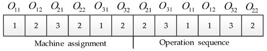
Figure 1.
Scheduling solution denotation.
4.2. Individual Position Vector
In our proposed IWOA, the individual position is still denoted as a multi-dimensional real vector, which also consists of two segments string with the size of mn, i.e., , where . The first segment denotes the information of machine assignment, and the second segment presents the information of operation sequencing. For the above 3 × 2 FJSP, the individual position vector can be represented by Figure 2, where element values are listed in the given order. In addition, the intervals are all set as , where presents the number of the jobs.
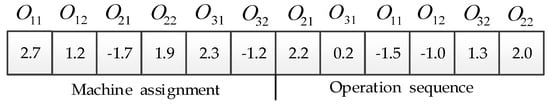
Figure 2.
Individual position vector.
4.3. Conversion Mechanism
Since the original WOA was proposed to tackle continuous problems, but the FJSP belongs to a discrete combinatorial problem, some measures should be implemented to construct the mapping relationship between the individual position vector and the discrete scheduling solution. In a previous study, Yuan et al. [10] proposed a method to implement the conversion between the continuous individual position vector and the discrete scheduling solution for the FJSP. Therefore, the conversion method in the literature [10] will be used in this study.
4.3.1. Conversion from Scheduling Solution to Individual Position Vector
For the machine assignment segment, the conversion process can be represented by Equation (19). Here, denotes the ith element of the individual position vector, presents the number of alternative machine set for the operation corresponding to the ith element, and means the serial number of the chosen machine in its alternative machine set; if , then can be achieved by choosing a random value in the interval .
For the operation sequence segment, firstly, it is needed to randomly generate mn real numbers in the range corresponding to the scheduling solution. According to the ranked-order-value (ROV) rule, a unique ROV value is assigned to each random number in an increasing order, so that each ROV value can correspond to an operation. Secondly, the ROV value is rearranged according to the coding order of the operations, and the random number corresponding to the rearranged ROV value is the value of the element of the individual position vector. The conversion process is shown in Figure 3.
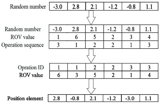
Figure 3.
The conversion process from operation sequence to individual position vector.
4.3.2. Conversion from Individual Position Vector to Scheduling Solution
For the machine assignment segment, according to the reverse derivation of Equation (19), the conversion can be achieved, which can be denoted by Equation (20).
For the operation sequence segment, the ROV value is firstly increasingly assigned to each element of the individual position vector, and then used as the Fixed ID. Therefore, a new operation sequence can be obtained by corresponding the ROV value to the operations, which is shown in Figure 4.
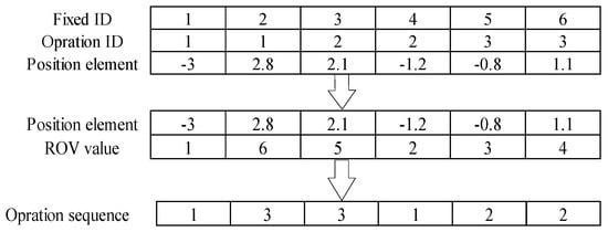
Figure 4.
The conversion from individual position vector to operation sequence.
4.4. Population Initialization
For a swarm intelligence optimization algorithm, the quality of the initial population is very crucial for the computational performance. In light of the characteristic of the FJSP, the population initialization process can be implemented in two phases. In the machine assignment phase, the better initial assignment schemes can be generated by utilizing a chaotic reverse learning method. In the operation sequence phase, some operation sequences are randomly generated. Combining each operation sequence with one of the initial assignment schemes, some scheduling solutions are generated and fitness function values of each scheduling solution are calculated. Then, the initial population can be achieved by choosing the scheduling solution with the best fitness value each time.
4.5. Nonlinear Convergence Factor
Like other swarm intelligence optimization algorithms, the coordination between the abilities of exploitation and exploration is important for the performance of the algorithm. In the original WOA, the abilities of exploitation and exploration mainly depend on the convergence factor . The larger the value of is, the stronger the ability of exploitation is, and then the WOA can exploit the optimal solution in a large space. The smaller the value of is, the stronger the ability of exploration is, and then it can merely explore the optimal solution in a small space. Therefore, for improving the efficiency of exploitation, the value of can be set to be larger in the early stage of iterations, which is beneficial to exploit the optimal solution in a larger space, and then it can be set to be smaller in the later stage of iterations, which is beneficial to concretely explore the better solution around the current optimal one. However, the value of linearly decreases over the course of iterations by Equation (13), which cannot improve the efficiency of the nonlinear search of the algorithm. Therefore, a nonlinear improvement of is adopted by Equation (21), where and denote the maximum iteration and current iteration, respectively.
4.6. Adaptive Weight
The improvement of can improve the optimization ability of the algorithm to some extent, but it cannot achieve the purpose of effectively balancing the abilities of exploitation and exploration. Therefore, the adaptive weight and the nonlinear convergence factor are cooperated to coordinate the abilities of exploitation and exploration of the algorithm. The adaptive weight proposed in the literature [32] is used to improve the optimization performance of the algorithm, with the formula shown by Equation (22), where and denote the maximum iteration and current iteration, respectively. The improved iterative formulas in the WOA can be defined by Equations (23) and (24).
4.7. Variable Neighborhood Search
In the local exploration phase, the whale individuals update their positions toward the current optimal individual using Equation (16). Therefore, determines the accuracy and effectiveness of the local exploration to some extent. Taking this into account, the variable neighborhood search strategy is used for improving the quality of the current optimal scheduling solution , and then the quality of the current optimal individual can be ameliorated as well. At the same time, an “iterative counter” is set for and assigned 0 at the initial moment. If does not change at each iteration, the “iterative counter” increases by 1; otherwise, it remains the same. When the “iterative counter” is equal to stability threshold Ts (15 in this paper), as the individuals reach the steady state, the variable neighborhood search strategy is performed on , allowing it to escape from the local optimum. For implementing the strategy, three neighborhood structures were designed as outlined below.
For the neighborhood structure , two random positions are chosen with different jobs in the second segment of the scheduling solution, exchanging the order of jobs from the second random position to the first random position.
For the neighborhood structure , two random positions are chosen with different jobs in the second segment of the scheduling solution, inserting the job of the first random position in the position behind the second random position.
For the neighborhood structure , a random position is chosen in the first segment of the scheduling solution, where the number of alternative machines is more than one, and then the current machine is replaced by another one of the alternative machines in the position.
The new scheduling solution is evaluated after each variable neighborhood search operation. If the new scheduling solution is better than the original one, then the new scheduling solution is set as the original one. The procedure of the variable neighborhood search operation can is illustrated in Algorithm 1.
| Algorithm 1. The procedure of VNS. |
| Step 1: Set the current optimal scheduling solution as the initial solution , where , , , and represents the maximum iteration, at the initial moment. |
| Step 2: If , set as ; if , set as ; if , set as ; represents the new scheduling solution, and represents employing the ith neighborhood structure operation on , where I = 1, 2, or 3. |
| Step 3: Set as , and then the local optimal scheduling solution can be obtained by executing the local search operation. |
| Step 4: If is better than , then set as , and set ; otherwise, set as . |
| Step 5: If , then set as , and go to step 6; otherwise, go to step 3. |
| Step 6: If , go to step 7; otherwise, go to step 2. |
| Step 7: End. |
In this study, the threshold acceptance method is used for the local search operation, which is shown as Algorithm 2.
| Algorithm 2. The procedure of the local search in VNS. |
| Step 1: Get the initial solution , and set , , , and maximum iteration . |
| Step 2: If , set as ; if , set as . |
| Step 3: If , then set as ; otherwise, set as . |
| Step 4: Set as , if , then set as , go to step 5; otherwise, go to step 2. |
| Step 5: End. |
4.8. The Procedure of the Proposed IWOA
The detailed steps of the proposed IWOA can be described as Algorithm 3.
| Algorithm 3. The procedure of IWOA. |
| Step 1: Set parameters and generate the initial population by utilizing the chaotic reverse learning strategy and search method. |
| Step 2 Calculate the fitness value of each scheduling solution in the population, and then find and retain the optimal scheduling solution . |
| Step 3: Judge whether the termination conditions can be met. If not met, perform steps 4–7; otherwise, perform step 8. |
| Step 4: Judge whether the value of the “iterative counter” is equal to 15. If met, go to step 5; otherwise, go to step 6. |
| Step 5: Employ the variable neighborhood search operation on , and update . |
| Step 6: Execute the conversion from scheduling solution to individual position vector, and retain the optimal individual position vector corresponding to |
| Step 7: Update each individual position vector using Equations (17), (23) and (24), and execute the conversion from individual position vector to scheduling solution; set , and then go to step 2. |
| Step 8: The algorithm ends and outputs the optimal scheduling solution . |
5. Experimental Results
5.1. Experimental Settings
To evaluate the performance of the proposed IWOA for solving the FJSP, the algorithm was coded in MATLAB 2016a and run on a computer configured with an Intel Core i5-8250 central processing unit (CPU) with 1.80 GHz frequency, 8 GB random-access memory (RAM), and a Windows 10 Operating System. Fifteen famous benchmarks that included a set of 10 instances taken from Brandimarte (BRdata) [33] and five instances taken from Kacem et al (KAdata) [34] were chosen to test the proposed algorithm. These benchmark instances were used by many researchers to estimate their approaches. For each benchmark instance, experimental simulations were run 20 times using different algorithms. After several preliminary experiments, the parameters of the proposed IWOA were set as follows: a population size of 100, maximum iterations of 1000, spiral constant b of one, and and both set to 10.
5.2. Effectiveness of the Improvement Strategies
In this paper, three strategies were employed to enhance the performance of the IWOA, i.e., CRL, NFC and AW, and VNS. In this subsection, the effectiveness of the three strategies is firstly evaluated. In Table 1, the first and second columns present the name and size of the problems, and computational data are listed in the following columns. “WOA” defines the original whale optimization algorithm. “IWOA-1” is the algorithm where the nonlinear convergence factor and adaptive weight are both applied to the WOA. “IWOA-2” is the whale optimization algorithm with the variable neighborhood search strategy introduced. “IWOA” is the presented algorithm in this study. In addition, “Best” represents the best result in the 20 runs. “Avg” means the average results value of the twenty runs. “Time” is the mean computational time (in seconds) in the 20 runs. “LB” denotes the optimal value of makespan found so far. Boldface denotes the best mean result in the 20 runs. To enhance the comparison, the same parameters were set for the compared algorithms; for instance, population size was 100 and maximum iterations were 1000.

Table 1.
Effectiveness analysis of improvement strategy. See Section 5.2 for column descriptions. WOA—whale optimization algorithm.
From the experimental result in Table 1, the following conclusions can be obtained: (1) in comparisons of the “Best” value, the IWOA algorithm was better than the other three algorithms, which obtained seven optimal values, outperforming IWOA-1 in 12 out of 15 instances, IWOA-2 in nine out of 15 instances, and WOA in 13 out of 15 instances; (2) in comparisons of the “Time” value, WOA spent a shorter time than the other three algorithms. Compared with IWOA-1, the increase in computation time was mainly the result of the addition of the variable neighborhood search operation in WOA, which led to increased time complexity of the algorithm; (3) in comparisons of the “Avg” value, the IWOA algorithm obtained all optimal values, outperforming WOA and IWOA-1 in 15 out of 15 instances, and outperforming IWOA-2 in 13 out of 15 instances.
5.3. Effectiveness of the Proposed IWOA
To demonstrate the effectiveness of the proposed IWOA, the second experiment was executed on KAdata. In Table 2, the proposed algorithm is compared with the knowledge-based ant colony optimization (KBACO) [35], hybrid tabu search algorithm (TSPCB) [36], and the hybrid gray wolf optimization algorithm (HGWO) [37]. The first column presents the name of the problems. “Best” represents the best makespan. “Avg” means the average makespan. “Time” is the mean computational time of the instance. “LB” denotes the optimal value of makespan found so far. “Avg-T“ is the mean computational time executed on KAdata. As can be seen, the proposed IWOA obtained three optimal values in solving KAdata, compared with five for ACO, five for HTS, and four for HGWO. However, the average computational time for the IWOA was very low, at only 4 s (on a Lenovo Thinkpad E480 with CPU i5-8250 @1.80GHz and 8 GB RAM) compared to 4978.8 s (in Matlab on a Dell Precision 650 workstation with a Pentium IV 2.4 GHz CPU and 1 GB RAM) for KBACO, 214.8 s (in C++ on a Pentium IV 1.6 GHz CPU and 512 MB RAM) for TSPCB, and 19 s (in Fortran on a Pentium CPU G2030@ 3.0 GHz and 2 GB ) for HGWO. Because the computers applied for running the programs was different, the comparison among the running times of different algorithms was difficult. However, even if there exists some differences in the speed between the processors involved, IWOA was obviously faster than the other three algorithms.
Table 2.
Comparison between the proposed improved WOA (IWOA) and existing algorithms on the KAdata. See Section 5.3 for column descriptions.
Another experiment was implemented on BRdata. Table 3 compares our proposed IWOA with the following six algorithms: KBACO [35], TSPCB [36], HGWO [37], artificial immune algorithm (AIA) [38], particle swarm optimization combined with tabu search (PSO+TS) [39], and tabu search metaheuristic with a new neighborhood structure called “golf neighborhood” (TS3) [40]. The first column stands for the name of the problems, and the second column represents the optimal value found so far. “Best” represents the best makespan. “Mean” represents the average result of “RPD” in the 20 runs. Boldface denotes the best result of “RPD” in the 20 runs. “RPD” represents the relative percentage deviation to “LB” and is calculated as follows:
Table 3.
Comparison between different algorithms on the BRdata.
As can be seen from Table 3, the following conclusions can be easily obtained: (1) in comparisons of the “Best” value, the proposed IWOA showed competitive performance on BRdata, obtaining four optimal values, outperforming KBACO in seven out of 10 instances, TS3 and PSO+TS in nine out of 10 instances, and HGWO in eight out of 10 instances, while it was equal to both AIA and TSPCB in six out of 10 instances; (2) in comparisons of the “RPD” value, the proposed IWOA obtained five optimal values, outperforming KBACO in seven out of 10 instances, both TS3 and PSO+TS in nine out of 10 instances, and HGWO in eight out of 10 instances, while it was inferior to both AIA and TSPCB in three out of 10 instances; (3) in comparisons of the “Mean” value, the value for the proposed IWOA was very low at only 4.91, outperforming the 5.65 for KBACO, 10.12 for HGWO, 23.89 for PSO+TS, and 13.34 for TS3, while it was inferior to the 2.78 for TSPCB and 2.22 for AIA. However, by comparison, the IWOA obtained the best values in an acceptable time.
6. Conclusions
In this paper, a novel improved whale optimization algorithm (IWOA), based on the integrated approach, was presented for solving the flexible job shop scheduling problem (FJSP) with the objective of minimizing makespan. The conversion method between the whale individual position vector and the scheduling solution was firstly proposed. After that, three improvement strategies were employed in the algorithm, namely chaotic reverse learning (CRL), the nonlinear convergence factor (NFC) and adaptive weight (AW), and the variable neighborhood search (VNS). The CRL was employed to ensure the quality of the initial solutions. The NFC and AW were introduced to balance the abilities of exploitation and exploration. The VNS was adopted to enhance the accuracy and effectiveness of the local exploration.
Extensive experiments based on 15 benchmark instances were executed. The effectiveness of improvement strategies was firstly certified by a number of experiments. Then, the proposed IWOA was compared with six recently published algorithms. According to the comparison results, the proposed IWOA can obtain better results in an acceptable time.
In the future, we will concentrate on a more complex FJSP, such as the energy-efficient flexible job shop scheduling problem, the multi-objective flexible job shop scheduling problem, or the dynamic flexible job shop scheduling problem. Meanwhile, other effective improvement strategies in WOA will be studied to further improve the capacity of the algorithm for this FJSP.
Author Contributions
Conceptualization, methodology and writing—original manuscript, F.L. (Fei Luan); project management, supervision and writing—review, Z.C. and T.J.; experiments and result analysis, S.W. and F.L. (Fukang Li); investigation, formal analysis and editing, J.Y.
Funding
This work was supported by the National Natural Science Foundation of China under Grant 11072192, the Project of Shaanxi Province Soft Science Research Program under Grant 2018KRM090, the Project of Xi’an Science and Technology Innovation Guidance Program under Grant 201805023YD1CG7(1), and the Shandong Provincial Natural Science Foundation of China under Grant ZR2016GP02.
Conflicts of Interest
The authors declare no conflicts of interest.
References
- Nowicki, E.; Smutnicki, C. A fast taboo search algorithm for the job shop problem. Manag. Sci. 1996, 42, 797–813. [Google Scholar] [CrossRef]
- Gonc, J.F.; Magalhaes Mendes, J.J.; Resende, M.G.C. A hybrid genetic algorithm for the job shop scheduling problem. Eur. J. Oper. Res. 2005, 167, 77–95. [Google Scholar]
- Lochtefeld, D.F.; Ciarallo, F.W. Helper-objective optimization strategies for the Job-Shop Scheduling Problem. Appl. Soft Comput. 2011, 11, 4161–4174. [Google Scholar] [CrossRef]
- Garey, M.R.; Johnson, D.S.; Sethi, R. The complexity of flow shop and job shop scheduling. Math. Oper. Res. 1976, 1, 117–129. [Google Scholar] [CrossRef]
- Brucker, P.; Schlie, R. Job-shop scheduling with multi-purpose machines. Computing 1990, 45, 369–375. [Google Scholar] [CrossRef]
- Dauzere-Peres, S.; Paulli, J. An integrated approach for modeling and solving the general multi-processor job-shop scheduling problem using tabu search. Ann. Oper. Res. 1997, 70, 281–306. [Google Scholar] [CrossRef]
- Mastrolilli, M.; Gambardella, L.M. Effective neighborhood functions for the flexible job shop problem. J. Sched. 2000, 3, 3–20. [Google Scholar] [CrossRef]
- Mati, Y.; Lahlou, C.; Dauzere-Peres, S. Modelling and solving a practical flexible job shop scheduling problem with blocking constraints. Int. J. Prod. Res. 2011, 49, 2169–2182. [Google Scholar] [CrossRef]
- Mousakhani, M. Sequence-dependent setup time flexible job shop scheduling problem to minimise total tardiness. Int. J. Prod. 2013, 51, 3476–3487. [Google Scholar] [CrossRef]
- Yuan, Y.; Xu, H.; Yang, J. A hybrid harmony search algorithm for the flexible job shop scheduling problem. Appl. Soft Comput. 2013, 13, 3259–3272. [Google Scholar] [CrossRef]
- Tao, N.; Hua, J. A cloud based improved method for multi-objective flexible job shop scheduling problem. J. Intell. Fuzzy Syst. 2018, 35, 823–829. [Google Scholar]
- Gong, G.L.; Deng, Q.W.; Gong, X.R. A new double flexible job shop scheduling problem integrating processing time, green production, and human factor indicators. J. Clean. Prod. 2018, 174, 560–576. [Google Scholar] [CrossRef]
- Wang, H.; Jiang, Z.G.; Wang, Y. A two-stage optimization method for energy-saving flexible job shop scheduling based on energy dynamic characterization. J. Clean. Prod. 2018, 188, 575–588. [Google Scholar] [CrossRef]
- Marzouki, B.; Driss, O.B.; Ghédira, K. Multi Agent model based on Chemical Reaction Optimization with Greedy algorithm for Flexible Job shop Scheduling Problem. Procedia Comput. Sci. 2017, 112, 81–90. [Google Scholar] [CrossRef]
- Yuan, Y.; Xu, H. Multiobjective flexible job shop scheduling using memetic algorithms. IEEE Trans. Autom. Sci. Eng. 2015, 12, 336–353. [Google Scholar] [CrossRef]
- Gao, K.Z.; Suganthan, P.N.; Pan, Q.K.; Chua, T.J.; Cai, T.X.; Chong, C.S. Discrete Harmony Search Algorithm for Flexible Job Shop Scheduling Problem with Multiple Objectives. J. Intell. Manuf. 2016, 27, 363–374. [Google Scholar] [CrossRef]
- Piroozfard, H.; Wong, K.Y.; Wong, W.P. Minimizing total carbon footprint and total late work criterion in flexible job shop scheduling by using an improved multi-objective genetic algorithm. Resour. Conserv. Recycl. 2018, 128, 267–283. [Google Scholar] [CrossRef]
- Jiang, T.H.; Zhang, C.; Zhu, H.Q.; Deng, G.L. Energy-Efficient scheduling for a job shop using grey wolf optimization algorithm with double-searching mode. Math. Probl. Eng. 2018, 2018, 1–12. [Google Scholar] [CrossRef]
- Singh, M.R.; Mahapatra, S. A quantum behaved particle swarm optimization for flexible job shop scheduling. Comput. Ind. Eng. 2016, 93, 36–44. [Google Scholar] [CrossRef]
- Wu, X.L.; Sun, Y.J. A green scheduling algorithm for flexible job shop with energy-saving measures. J. Clean. Prod. 2018, 172, 3249–3264. [Google Scholar] [CrossRef]
- Jiang, T.; Zhang, C. Application of grey wolf optimization for solving combinatorial problems: job shop and flexible job shop scheduling cases. IEEE Access 2018, 6, 26231–26240. [Google Scholar] [CrossRef]
- Jiang, T.H.; Deng, G.L. Optimizing the low-carbon flexible job shop scheduling problem considering energy consumption. IEEE. Access 2018, 6, 46346–46355. [Google Scholar] [CrossRef]
- Jiang, T.H.; Zhang, C.; Sun, Q. Green job shop scheduling problem with discrete whale optimization algorithm. IEEE Access 2019, 7, 43153–43166. [Google Scholar] [CrossRef]
- Li, X.Y.; Gao, L. An effective hybrid genetic algorithm and tabu search for flexible job shop scheduling problem. Int. J. Prod. Econ. 2016, 174, 93–110. [Google Scholar] [CrossRef]
- Mirjalili, S.; Lewis, A. The whale optimization algorithm. Adv. Eng. Soft. 2016, 95, 51–67. [Google Scholar] [CrossRef]
- Aljarah, I.; Faris, H.; Mirjalili, S. Optimizing connection weights in neural networks using the whale optimization algorithm. Soft. Comput. 2018, 22, 1–15. [Google Scholar] [CrossRef]
- Mafarja, M.M.; Mirjalili, S. Hybrid whale optimization algorithm with simulated annealing for feature selection. Neurocomputing 2017, 260, 302–312. [Google Scholar] [CrossRef]
- Aziz, M.A.E.; Ewees, A.A.; Hassanien, A.E. Whale optimization algorithm and moth-flame optimization for multilevel thresholding image segmentation. Expert Syst. Appl. 2017, 83, 242–256. [Google Scholar] [CrossRef]
- Oliva, D.; Aziz, M.A.E.; Hassanien, A.E. Parameter estimation of photovoltaic cells using an improved chaotic whale optimization algorithm. Appl. Energy 2017, 200, 141–154. [Google Scholar] [CrossRef]
- Jiang, T.H.; Zhang, C.; Zhu, H.Q.; Zhu, H.Q.; Gu, J.C.; Deng, G.L. Energy-efficient scheduling for a job shop using an improved whale optimization algorithm. Mathematics 2018, 6, 220. [Google Scholar] [CrossRef]
- Abdel-Basset, M.; Manogaran, G.; El-Shahat, D.; Mirjalili, S.; Gunasekaran, M. A hybrid whale optimization algorithm based on local search strategy for the permutation flow shop scheduling problem. Future Gener. Comput. Syst. 2018, 85, 129–145. [Google Scholar] [CrossRef]
- Guo, Z.Z.; Wang, P.; Ma, Y.F.; Wang, Q.; Gong, C.Q. Whale optimization algorithm based on adaptive weights and cauchy variation. Micro Comput. 2017, 34, 20–22. (In Chinese) [Google Scholar]
- Brandimarte, P. Routing and scheduling in a flexible job shop by tabu search. Ann. Oper. 1993, 41, 157–183. [Google Scholar] [CrossRef]
- Kacem, I.; Hammadi, S.; Borne, P. Correction to “Approach by localization and multiobjective evolutionary optimization for flexible job-shop scheduling problems”. IEEE Trans. Syst. Man Cybern. Part C 2002, 32, 172. [Google Scholar] [CrossRef]
- Xing, L.N.; Chen, Y.W.; Wang, P.; Zhao, Q.S.; Xiong, J. A knowledge-based ant colony optimiztion for flexible job shop scheduling problems. Appl. Soft Comput. 2010, 10, 888–896. [Google Scholar] [CrossRef]
- Li, J.Q.; Pan, Q.K.; Suganthan, P.N.; Chua, T.J. A hybrid tabu search algorithm with an efficient neighborhood structure for the flexible job shop scheduling problem. Int. J. Adv. Manuf. Technol. 2011, 52, 683–697. [Google Scholar] [CrossRef]
- Jiang, T.H. A hybrid grey wolf optimization algorithm for solving flexible job shop scheduling problem. Control Decis. 2018, 33, 503–508. (In Chinese) [Google Scholar]
- Bagheri, A.; Zandieh, M.; Mahdavi, I.; Yazdani, M. An artificial immune algorithm for the flexible job-shop scheduling problem. Future Gener. Comput. Syst. 2010, 26, 533–541. [Google Scholar] [CrossRef]
- Henchiri, A.; Ennigrou, M. Particle Swarm Optimization Combined with Tabu Search in a Multi-Agent Model. for Flexible Job Shop Problem; Springer Nature: Basingstoke, UK, 2013; Volume 7929, pp. 385–394. [Google Scholar]
- Bozejko, W.; Uchronski, M.; Wodecki, M. The New Golf Neighborhood for the Flexible Job Shop Problem; ICCS, Elsevier Series; Elsevier: Amsterdam, The Netherlands, 2010; pp. 289–296. [Google Scholar]
© 2019 by the authors. Licensee MDPI, Basel, Switzerland. This article is an open access article distributed under the terms and conditions of the Creative Commons Attribution (CC BY) license (http://creativecommons.org/licenses/by/4.0/).