Methods for Assessing Human–Machine Performance under Fuzzy Conditions

Abstract

The assessment of a system’s performance is a very important task, enabling its designer/user to correct its weaknesses and make it more effective. Frequently, in practice, a system’s assessment is performed under fuzzy conditions, e.g., using qualitative instead of numerical grades, incomplete information about its function, etc. The present review summarizes the author’s research on building assessment models for use in a fuzzy environment. Those models include the measurement of a fuzzy system’s uncertainty, the application of the center of gravity defuzzification technique, the use of triangular fuzzy or grey numbers as assessment tools, and the application of the fuzzy relation equations. Examples are provided of assessing human (students and athletes) and machine (case-based reasoning systems in computers) capacities, illustrating our results. The outcomes of those examples are compared to the outcomes of the traditional methods of calculating the mean value of scores assigned to the system’s components (system’s mean performance) and of the grade point average index (quality performance) and useful conclusions are obtained concerning their advantages and disadvantages. The present review forms a new basis for further research on systems’ assessment in a fuzzy environment.

1. Introduction

In the language of management, a system is understood to be a set of interacting components forming an integrated whole and working together for achieving a common target (e.g., maximum profit, low cost of production, healthcare, student learning, etc.). One can distinguish among physical, biological, social, economic, engineering, abstract knowledge, etc. systems. The evaluation of a system’s performance constitutes an important topic of the system general theory [1], because it enables the correction of its weaknesses, resulting in the improvement of its effectiveness in the environment of a given situation.

A system assessment is frequently performed under fuzzy conditions, caused by incomplete information about its function and characteristics, using qualitative (linguistic) assessment grades, or various other reasons appearing in real life situations. Several efforts have been reported in the literature for the assessment under fuzzy conditions (e.g., see [2,3,4,5,6]). The purpose of the present work is to review its author’s research on building assessment models for use in a fuzzy environment.

The rest of the article is formulated as follows. Section 2 provides a brief account of the evolution of fuzzy set theory and its generalizations and its connection to fuzzy logic. In Section 3, the use of fuzzy system uncertainty is utilized as an assessment method of its effectiveness, whereas, in Section 4, the same is done with the center of gravity defuzzification technique, the outcomes of which are compared to those of the traditional method of calculating the grade point average index. In Section 5 and Section 6, assessment models using as tools triangular fuzzy numbers and grey numbers, respectively, are developed and compared to each other. The use of fuzzy relation equations for assessing mathematical modeling skills is the objective of Section 7 and the article closes with Section 8 containing the general conclusions of the review and some hints for future research.

The present review provides a new framework for research on a system’s evaluation under fuzzy conditions.

2. Fuzzy Sets and Generalizations

The “Laws of Thought” [7], of Aristotle (384–322 BC, Figure 1) that dominated for centuries the human reasoning are the following:

• The principle of identity
• The law of the excluded middle
• The law of contradiction

The law of the excluded middle (i.e., yes or no) was the basis for the traditional bi-valued logic and the precision of the classical mathematics owes undoubtedly a large part of its success to it. However, there were also strong objections to this law. The Buddha Siddhartha Gautama, who lived in India a century earlier, had already argued that almost every notion contains elements from its opposite one, while Plato (427–377 BC, Figure 1) discussed the existence of a third area beyond “true” and “false”, where these two opposite notions can exist together. Modern philosophers including Hegel, Marx, and Engels adopted and further cultivated the above belief.

The Polish philosopher Jan Lukasiewicz (1878–1956) first proposed a systematic alternative of the bi-valued logic introducing in the early 1900s a three-valued logic by adding the term “possible” between “true” and “false” [8]. Eventually, he developed an entire notation and axiomatic system from which he hoped to derive modern mathematics. Later, he also proposed four- and five-valued logics and then finally arrived at the conclusion that, axiomatically, nothing could prevent the derivation of an infinite valued Logic. Similar ideas were also expressed by the famous Polish-American logician and mathematician Alfred Tarski (1901–1983) [9].

However, it was not until relatively recently that an infinite-valued logic was introduced, called Fuzzy Logic (FL) [10], because it is based on the notion of Fuzzy Set (FS) initiated in 1965 by Lotfi Aliasker Zadeh (1921–2017, Figure 2) [11], an electrical engineer of Iranian origin, born in Azerbaijan, USSR and Professor at the University of Berkeley, California. A fuzzy subset A of the set of the discourse U (or, for brevity, a FS in U) is defined by A = {(x, m_A(x)): x ∈ U}, where m_A: U → [0, 1] is its membership function. The real number m_A(x) is called the membership degree of x in A. The greater is m_A(x), the more x satisfies the characteristic property of A. Many authors, for reasons of simplicity, identify it with the function m_A.

A crisp subset B of U can be considered as a special case of a FS in U with membership function ${\mathrm{m}}_{\mathrm{B}}(\mathrm{x})=\{\begin{array}{c}1,\mathrm{x}\in \mathrm{B}\\ 0,\mathrm{x}\notin \mathrm{B}\end{array}$. Based on this, most notions and operations concerning the crisp sets, e.g., subset, complement, union, intersection, Cartesian product, binary and other relations, etc., can be extended to FS. For information on FS, we refer to the book [12].

Through FL, the fuzzy terminology is translated by algorithmic procedures into numerical values, operations are performed upon those values and the outcomes are returned into natural language statements in a reliable manner. As expected, this far-reaching theory aroused some objections in the scientific community. Haack [13] argued that it can be shown that FL is unnecessary in all cases. Fox [14] responded to her objections claiming that FL is useful for handling real-world situations that are inherently fuzzy, calculating the existence in such situations fuzzy data and describing the operation of the corresponding fuzzy systems. He indicated that traditional and FL theories need not be seen as competitive, but as complementary and that FL, despite the objections of classical logicians, has proved very successful in practical applications in almost all sectors of human activity (e.g., see [12] (Chapter 6), [15,16,17,18,19]).

It must be mentioned here that fuzzy mathematics has also been significantly developed on the theoretical level, providing important contributions even in branches of classical mathematics, such as algebra, analysis, geometry, etc. FL constitutes one of the three portals of computational intelligence, which is a topic of the wide field of artificial intelligence. The other two portals of computational intelligence are neural networks and the evolutionary computing.

Several efforts have been made to improve and generalize the FS theory. Atanassov introduced in 1986, as a complement of Zadeh’s membership degree (M), the degree of non-membership (N) and defined the intuitionistic FS [20]. Smarandache introduced in 1995 the degree of indeterminacy/neutrality (I) and defined the neutrosophic set in three components (M, N, I), where M, N and I are subsets of the interval [0, 1] [21]. Alternatives to the FS theory were proposed by Deng in 1982 (Grey Systems [22]), Pawlak in 1991 (Rough Sets [23]), Molodtsov in 1999 (Soft Sets [24]) and others. Principles of the Grey System (GS) theory are used in Section 6.

3. Types of Uncertainty in Fuzzy Systems

Uncertainty can be defined as the shortage of precise knowledge and complete information on data that describe the state of the corresponding system. According to a fundamental principle of classical information theory, a system’s uncertainty is connected to its ability to obtain new information. Therefore, the measurement of the uncertainty could be used as a method for evaluating a system’s mean performance.

Shannon introduced in 1948 a formula for measuring the uncertainty and the information connected to it, which is based on the laws of classical probability and it is widely known as Shannon’s entropy [25]. This term comes from the mathematical definition of information when we have equally probable cases for the evolution of the corresponding phenomenon: $-\frac{\Delta (\log P)}{\log 2}$, where P is the probability of appearance of each case. This expression appears to be analogous to a well-known formula from physics: ΔS = $\frac{\Delta Q}{T}$, where ΔS is the increase of a physical system’s entropy caused by an increase of the heat ΔQ, when the absolute temperature T remains constant.

Let U denote the universal set of the discourse. For use in a fuzzy environment, Shannon’s formula (probabilistic uncertainty) has been adapted [26] (p.20) to the form:

$$\mathrm{H}=-\frac{1}{\ln n}{\displaystyle \sum _{s=1}^n{m}_s\ln }{m}_s.$$

(1)

In Equation (1), m_s = m(s) denotes the membership degree of the element s of U in the corresponding fuzzy set and n denotes the total number of the elements of U. Dividing the sum by ln n, one makes H take values in the interval [0, 1].

The fuzzy probability of an element s of U is defined by

$$P_s=\frac{m_s}{{\displaystyle \sum _{s\in U}{m}_s}}$$

(2)

However, according to the British economist Shackle [27] and many other researchers after him, human reasoning can be formulated more adequately by the possibility rather than by the probability theory. The possibility, e.g., r_s, of an element s of U is defined by

$$r_s=\frac{m_s}{\max \left\{m_s\right\}}$$

(3)

In Equation (3), max{m_s} denotes the maximal value of m_s, for all s in U. In other words, the possibility of s expresses the relative membership degree of s with respect to max {m_s}.

In terms of possibility, the uncertainty is measured by the sum of strife (or discord) and non-specificity (or imprecision). The former is connected to the conflict created among the membership degrees, whereas the latter is connected to the conflict created among the cardinalities (sizes) of the various fuzzy subsets of U [26] (p.28). Note that the cardinality of a fuzzy subset of U is defined sa the sum ${\displaystyle \sum _{x\in U}m(x)}$ of all membership degrees of the elements of U with respect to it.

The following example illustrates this situation.

Example 1.

Let U be the set of all mountains of a country and let H and L be its fuzzy subsets of the high and low mountains with membership functions m_H and m_L, respectively. Assume further that a mountain x in U has a height of 1000 m.

Then, strife is created by the existing conflict between the membership degrees m_H(x) and m_L(x). In fact, if the country has high mountains in general, then m_H(x) should take values near 0 and m_l(x) near 1. However, the opposite could happen, if the country has low mountains in general.

On the other hand, non-specificity is connected to the question of how many elements of U should have zero membership degrees with respect to H and L.

Strife is measured [26] (p.28) by the function ST(r) on the ordered possibility distribution r: r₁ = 1 $\ge$ r₂ $\ge$ …… $\ge$ r_n $\ge$ r_n+1 of a group of the elements of U defined by

$$ST(r)=\frac{1}{\log 2}[{\displaystyle \sum _{i=2}^m(r_i-r_{i+1})\log \frac{i}{{\displaystyle \sum _{j=1}^i{r}_j}}}].$$

(4)

Under the same conditions non-specificity is measured [26] (p.28) by the function

$$N(r)=\frac{1}{\log 2}[{\displaystyle \sum _{i=2}^m(r_i-r_{i+1})\log i}].$$

(5)

The sum T(r) = ST(r) + N(r) measures the fuzzy system’s total possibilistic uncertainty.

Example 2.

Table 1. Student results.

Grade	G1	G2
A	1	10
B	13	6
C	4	3
D	3	0
F	0	1
Total	21	20

depicts the performance of two equivalent student groups in a common test with respect to the linguistic grades, where A = excellent, B = very good, C = good, D = fair and F = unsatisfactory:

It is asked to evaluate the performance of the two student groups by calculating the total possibilistic and probabilistic uncertainty existing in them.

(i) Total possibilistic uncertainty: Defining the membership function in terms of the frequencies of the student grades, one can represent the two student groups as fuzzy sets on the set U = {A, B, C, D. F} in the form {(x, $\frac{n_x}{n}$): x $\in$ U }, where n_x is the number of students who received the grade x and n is the total number of the students in each group. In other words, we can write

• G₁ = {(A, $\frac{1}{21}$), (B, $\frac{13}{21}$), (C, $\frac{4}{21}$), (D, $\frac{3}{21}$), (F, 0) }; and
• G₂ = {(A, $\frac{10}{20}$), (B, $\frac{6}{20}$), (C, $\frac{3}{20}$), (D, 0), (F, $\frac{1}{20}$) }.

The maximal membership degree in G₁ is equal to $\frac{13}{21}$, hence the possibilities of the elements of U in G₁ are: r(A) =$\frac{1}{13}$, r(B) = 1, r(C) =$\frac{4}{13}$, r(D) = $\frac{3}{13}$, r(F) = 0. Therefore, the ordered possibility distribution defined on G₁ is

$$\mathit{r}:r_1=1>r_2=\frac{4}{13}>r_3=\frac{3}{13}>r_4=\frac{1}{13}>r_5=0.$$

(6)

Similarly, one finds that the ordered possibility distribution on G₂ is:

$$\mathit{r}:r_1=1>r_2=\frac{6}{10}>r_3=\frac{3}{10}>r_4=\frac{1}{10}>r_5=0.$$

(7)

Equation (4) gives in our case that

$$ST(r)=\frac{1}{\log 2}[(r_2-r_3)\log \frac{2}{r_1+r_2}+(r_3-r_4)\log \frac{3}{r_1+r_2+r_3}+(r_4-r_5)\log \frac{4}{r_1+r_2+r_3+r_4}]$$

Replacing the values of the possibility distribution r from Equation (6), one finds for G₁ that

$$ST(r)=\frac{1}{\log 2}[\frac{1}{13}\log (\frac{26}{17})+\frac{2}{13}\log (\frac{39}{20})+\frac{1}{13}\log (\frac{42}{21})]\approx 0.27.$$

In addition, Equation (5) gives for G₁ that

$$N(r)=\frac{1}{\log 2}[\frac{1}{13}\log 2+\frac{2}{13}\log 3+\frac{1}{13}\log 4]\approx 0.48$$

Therefore, the total possibilistic uncertainty for G₁ is T (r) $\approx$ 0.27 + 0.48 = 0.75.

In the same way, replacing the values of r from Equation (7), one finds that the total possibilistic uncertainty for G₂ is T (r) $\approx$ 0.33 + 0.82 = 1.15.

Since the two student groups have been chosen to be equivalent, they have the same existing uncertainty before the test. Thus, the reduction of uncertainty is greater for Group G₁, which therefore demonstrates a better mean performance than Group G₂.

(ii) Probabilistic uncertainty: Substituting the membership degrees of G₁ into Equation (1), one finds that the probabilistic uncertainty for the experimental group is equal to:

$$\mathrm{H}=-\frac{1}{\ln 5}(\frac{1}{21}\ln \frac{1}{21}+\frac{13}{21}\ln \frac{13}{21}+\frac{4}{21}\ln \frac{4}{21}+\frac{3}{21}\ln \frac{3}{21})\approx 0.64.$$

Similarly, one finds that for G₂ the probabilistic uncertainty is approximately equal to 0.71. Therefore, Group G₁ demonstrates again a better performance.

Remark 1.

From the previous example, it becomes evident that the measurement of uncertainty can be used for assessing the performance of the two groups only under the assumption that they are equivalent, which means that they have the same existing uncertainty before the test.

4. The Center of Gravity Defuzzification Technique

The process of solving a problem with principles and methods of FL involves the following phases:

• Choose the suitable universal set.
• Fuzzify the given data by defining suitable membership functions for the FSs involved in this procedure.
• Elaborate the fuzzy data with FL techniques for expressing the solution of the given problem in the form of a unique FS.
• Defuzzify the above FS by representing it with a real numerical value to “translate” the problem’s solution into the natural language.

There are more than 30 defuzzification methods in use, but two of them are the most popular. In the Maximum method, the crisp value representing the solution’s output is one of the values at which the corresponding FS has its maximum truth (e.g., [15] (Chapter 4, pp. 97–99)). On the other hand, in the Center of Gravity (COG) technique, the representative crisp value is obtained by calculating the coordinates of the COG of the level’s area S between the graph of the membership function of the corresponding FS and the OX axis [28].

Voskoglou [29] developed in 1999 a fuzzy model for representing mathematically the process of learning a subject matter in the classroom and later, considering the class as a fuzzy system, he calculated its existing uncertainty (see Section 3) for assessing the student mean performance [30]. Subbotin et al. [31], based on the Voskoglou’s model, adapted properly the COG defuzzification technique for use as an assessment method of student learning skills. Since then, Subbotin and Voskoglou applied jointly or separately the COG method, termed as Rectangular Assessment Model (RFAM), in many other types of assessment problems (e.g., see [15] (Chapter 6)). Here, we present the headlines of RFAM and we compare it to the traditional assessment method of calculating the Grade Point Average (GPA) index.

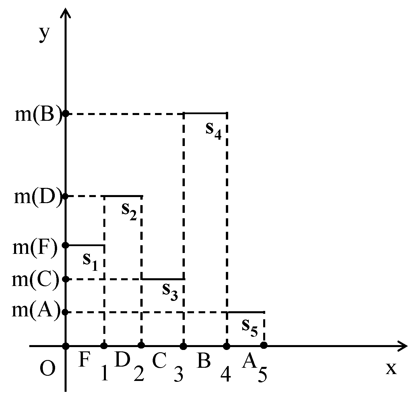
4.1. The Rectangular Fuzzy Assessment Model

We choose, exactly as in Example 2, for discourse the set of linguistic grades U = {A, B, C, D, F} and we represent a student group G as a FS in U in the form G = {(x, $\frac{n_x}{n}$): x $\in$ U }, where n is the total number of the students of G and n_x is the number of students of G whose performance is characterized by the grade x in U.

To be able to design the graph of the membership function y = m(x), we replace U with a set of real intervals as: F $\to$ [0, 1), D $\to$ [1, 2), C $\to$ [2, 3), B $\to$ [3, 4), A $\to$ [4, 5]. Consequently, we have that y₁ = m(x) = m(F) for all x in [0, 1), y₂ = m(x) = m(D) for all x in [1, 2), y₃ = m(x) = m(C) for all x in [2, 3), y₄ = m(x) = m(B) for all x in [3, 4) and y₅ = m(x) = m(A) for all x in [4, 5). Since the membership values of the elements of U in G have been defined in terms of the corresponding frequencies, we obviously have that: ${\displaystyle \sum _{i=1}^5{y}_i}$ = m(A) + m(B) + m(C) + m(D) + m(F) = 1.

The graph of the membership function y = m(x) is shown in Figure 3, where the level’s area S between the graph and the OX axis is equal to the sum of the areas of the five rectangles S_i, i = 1, 2, 3, 4, 5, one side of which has length 1 and lies on the OX axis. That is why this method was termed as RFAM.

The COG coordinates (x_c, y_c) are calculated by the well known from mechanics formulas:

$$x_c=\frac{{\displaystyle \underset{S}{\iint }xdxdy}}{{\displaystyle \underset{S}{\iint }dxdy}},y_c=\frac{{\displaystyle \underset{S}{\iint }ydxdy}}{{\displaystyle \underset{S}{\iint }dxdy}}$$

(8)

Here, we have that: ${\displaystyle \underset{S}{\iint }dxdy}$ $={\displaystyle \sum _{i=1}^5{y}_i=1}$. In addition, ${\displaystyle \underset{S}{\iint }xdxdy}={\displaystyle \sum _{i=1}^5{\displaystyle \underset{F_i}{\iint }xdxdy}}={\displaystyle \sum _{i=1}^5{\displaystyle \underset{0}{\overset{y_i}{\int }}dy}{\displaystyle \underset{i-1}{\overset{i}{\int }}xdx}}$ $={\displaystyle \sum _{i=1}^5{y}_i{\displaystyle \underset{i-1}{\overset{i}{\int }}xdx=}}$ $\frac{1}{2}{\displaystyle \sum _{i=1}^5(2i-1)y_i}$ and ${\displaystyle \underset{S}{\iint }ydxdy}$ = ${\displaystyle \sum _{i=1}^5{\displaystyle \underset{F_i}{\iint }ydxdy}}={\displaystyle \sum _{i=1}^5{\displaystyle \underset{0}{\overset{y_i}{\int }}ydy}{\displaystyle \underset{i-1}{\overset{i}{\int }}dx}}$ = ${\displaystyle \sum _{i=1}^n{\displaystyle \underset{0}{\overset{y_i}{\int }}ydy=\frac{1}{2}}}{\displaystyle \sum _{i=1}^n{y_i}^2}$.

Substituting the above values of the double integrals into Equation (8), one finds that

$$\begin{array}{l}{x}_C=\frac{1}{2}(y_1+3y_2+5y_3+7y_4+9y_5)\\ y_C=\frac{1}{2}({y_1}^2+{y_2}^2+{y_3}^2+{y_4}^2+{y_5}^2)\end{array}$$

(9)

However, (y_i − y_j)² = y_i² + y_j² − 2 y_ij ≥ 0, or y_i² + y_j² ≥ 2 y_ij for i, j = 1, 2, …, 5, with the equality holding if, and only if, y₁ = y₂ = y₃ = y₄ = y₅. Therefore, 1 = $({\displaystyle \sum _{i=1}^5{y}_i{)}^2}$ = ${\displaystyle \sum _{i=1}^n{y_i}^2}+2(y_1{y}_2+y_1{y}_3+\dots +y_4{y}_5)\ge 5{\displaystyle \sum _{i=1}^n{y_i}^2}$, or y₁² + y₂² + y₃² + y₄² + y₅² $\le \frac{1}{5}$, with the equality holding if and only if y₁ = y₂ = y₃ = y₄ = y₅ = $\frac{1}{5}$. Thus, Equation (9) shows that the unique minimum y_c = $\frac{1}{10}$ corresponds to the COG F_m ($\frac{5}{2}$, $\frac{1}{10}$).

The ideal case is when y₁ = y₂ = y₃ = y₄ = 0 and y₅ = 1. Then, from Equation (9), one finds that x_c = $\frac{9}{2}$ and y_c = $\frac{1}{2}$. Therefore, the COG in this case is the point F_i ($\frac{9}{2}$, $\frac{1}{2}$).

On the other hand, the worst case is when y₁ = 1 and y₂ = y₃ = y₄ = y₅ = 0. Therefore, from Equation (9), one finds that the COG is the point F_X ($\frac{1}{2}$, $\frac{1}{2}$).

Consequently, the area where COG F_c lies is the triangle F_xF_m F_i of Figure 4.

By making elementary observation on Figure 4, one obtains the following criterion for comparing the performance of two student groups:

• The group with the greater value of x_c demonstrates the better performance.
• In the case of the same value of x_c, if x_c ≥ 2.5, then the group with the greater value of y_c performs better. On the contrary, if x_c < 2.5, then the group with the lower value of y_c demonstrates the better performance.

Observe that a group’s performance depends mainly on the value of x_c, while the first part of Equation (9) shows that for the calculation of x_c greater coefficients are assigned to the higher scores. Therefore, the COG method focuses on the group’s quality performance.

In addition, since the ideal group’s performance corresponds to the value x_c = $\frac{9}{2}$, values greater than $\frac{9}{2}:2$ = 2.25 could be considered as demonstrating a satisfactory performance.

4.2. Comparison of the RFAM with the GPA Index

Keeping the same notation as in Section 4.1, the GPA index [15] (Chapter 6, p.125) is calculated by the formula

$$\mathrm{GPA}=\frac{0n_F+1n_D+2n_C+3n_B+4n_A}{n}$$

(10)

In other words, since greater coefficients (weights) are assigned to the higher scores, GPA is a weighted average connected to the group’s quality performance. In the case of the worst performance (n_F = n), Equation (10) gives that GPA = 0, while, in the case of the ideal performance (n_A = n), it gives that GPA = 4. Therefore, we have in general that 0 $\le$ GPA $\le$ 4. Consequently, values of GPA greater than 2 could be considered as indicating a satisfactory performance.

Equation (10) can be also written with respect to the frequencies in the form

GPA = y₂ + 2y₃ + 3y₄ + 4y₅.

(11)

Therefore, x_c = $\frac{1}{2}$ (y₁ + 3y₂ + 5y₃ + 7y₄ + 9y₅) = $\frac{1}{2}$(2GPA + 1), or

x_c = GPA + 0.5.

(12)

As an immediate consequence of Equation (12) and the first case of the assessment criterion in Section 4.1, if the values of the GPA index are different for two groups, then the GPA index and the RFAM provide the same assessment outcomes for those groups. The following example, due to Subbotin [32], shows that, in the case of the same GPA values, the application of the GPA index cannot lead to logically-based conclusions. Therefore, in such situations, the criterion in Section 4.1 becomes useful due to its logical nature.

Example 3.

The student grades of two classes with 60 students in each class are depicted in

Table 2. Student Grades.

Grades	Class I	Class II
C	10	0
B	0	20
A	50	40

.

The GPA index for the two classes is equal to $\frac{2\times 10+4\times 50}{60}=\frac{3\times 20+4\times 40}{60}\approx 3.67$, which means that the two classes demonstrate the same performance. However, Equation (12) gives that x_c = 4.17 for both classes. However, ${\displaystyle \sum _{i=1}^5{y_i}^2}$ = ${(\frac{1}{6})}^2+{(\frac{5}{6})}^2=\frac{26}{36}$ for the first and ${\displaystyle \sum _{i=1}^5{y_i}^2}$ = ${(\frac{2}{6})}^2+{(\frac{4}{6})}^2$ = $\frac{20}{36}$ for the second class. Therefore, according to the second case of the assessment criterion in Section 4.1, the first class demonstrates a better performance in terms of the RFAM.

Observe now that the ratio of the students receiving B or better to the total number of students is equal to $\frac{5}{6}$ for the first class and 1 for the second class, which means that Class II demonstrates a better quality performance. However, many educators might prefer the situation in Class I having a greater number of excellent students. Conclusively, in no case is it logical to accept that the two classes demonstrate the same performance, as the equal values of the GPA index indicate.

5. Triangular Fuzzy Numbers

5.1. Preliminaries

Fuzzy Numbers (FNs), introduced by Zadeh [33], play an important role in fuzzy mathematics, analogous to the role of ordinary numbers in classical mathematics. A FN, e.g., A, is defined to be a FS on the set R of real numbers, such that:

• A is normal, i.e., there exists x in R such that m_A(x) = 1.
• A is convex, i.e., all its a-cuts A^a = {x ∈ R: m_A (x) ≥ a}, with a in [0, 1], are closed real intervals.
• Its membership function y = m(x) is a piecewise continuous function.

One can define the basic arithmetic operations on FNs in two, equivalent to each other, ways:

(i) With the help of their a-cuts and the representation–decomposition theorem of Ralesscou-Negoita [34] (Theorem 2.1, p.16) stating that FS A can be completely and uniquely expressed by the family of its a-cuts in the form $\mathrm{A}={{\displaystyle \sum _{a\in [0,1]}a\mathrm{A}}}^a$.

(ii) By applying the Zadeh’s extension principle [12] (Section 1.4, p.20), which provides the means for any function f mapping the crisp set X to the crisp set Y to be generalized to map fuzzy subsets of X to fuzzy subsets of Y.

However, the above two general methods of the fuzzy arithmetic, requiring laborious calculations, are rarely used in practical applications, where the utilization of simpler forms of FNs is preferred.

A Triangular Fuzzy Number (TFN) (a, b, c), with a, b, and c real numbers such that a < b < c is the simplest form of a FN representing mathematically the fuzzy statement that “the value of b lies in the interval [a, c]”. The membership function y = m(x) of (a, b, c) is zero outside the interval [a, c], whereas its graph in [a, c] forms a triangle with the OX axis (Figure 5). Therefore, we have:

$$y=m(x)=\{\begin{array}{l}\frac{x-a}{b-a},x\in [a,b]\\ \frac{c-x}{c-b},x\in [b,c]\\ 0,x<aorx>c\end{array}$$

The coordinates (X, Y) of the Center of Gravity (COG) of the graph of the TFN A = (a, b, c), being the intersection point G of the medians AN and BM of the triangle ABC (Figure 5), are calculated by the formulas

$$\mathrm{X}(\mathrm{A})=\frac{a+b+c}{3},\mathrm{Y}(\mathrm{A})=\frac{1}{3}.$$

(13)

In fact, since M(, 0) and N($\frac{b+c}{2},\frac{1}{2}$), the proof is easily obtained by calculating the equations of the medians AN and BM and by solving their linear system.

According to the COG technique the first part of Equation (6) can be used to defuzzify the TFN A.

The two general methods for defining arithmetic operations on FNs lead to the following simple rules for the addition and subtraction of TFNs:

Let A = (a, b, c) and B = (a₁, b₁, c₁) be two TFNs. Then:

• The sum A + B = (a+a₁, b+b₁, c+c₁).
• The difference A – B = A + (–B) = (a – c₁, b – b₁, c – a₁), where –B = (–c₁, –b₁, –a₁) is defined to be the opposite of B.

On the contrary, the product and the quotient of A and B are FNs, which are not TFNs in general, apart from some special cases.

The following two scalar operations can also be defined:

• k + A = (k + a, k + b, k + c), k ∈ R.
• kA = (ka, kb, kc), if k > 0 and kA = (kc, kb, ka), if k < 0, k ∈ R.

Remark 2.

Another simple form of FNs that we have used as assessment tools [17] (Chapter 7) are the Trapezoidal Fuzzy Numbers (TpFNs). The membership function of a TpFN (a, b, c, d), with a, b, c, and d in R such that a < b ≤ c < d, is zero outside the interval [a, d], whereas its graph in [a, d] forms a trapezoid with the OX axis. The TFN (a, b, d) is a special case of the TpFN (a, b, c, d) with b = c, i.e., the TpFNs are actually generalizations of the TFNs.

For general information on FNs, we refer to the book [35].

5.2. The Assessment Method Using TFNs

In [36], we developed with the help of TFNs a method for assessing a system’s mean performance, whose steps are the following:

• Define the mean value of a finite number of given TFNs A₁, A₂, …, n ≥ 2, to be the TFN A = $\frac{1}{\mathrm{n}}$(A₁ + A₂ + … + A_n).
• Assign a scale of numerical scores from 1 to 100 to the linguistic grades A = excellent, B = very good, C = good, D = fair and F = unsatisfactory as follows: A (85–100), B (75–84), C (60–74), D (50–59) and F (0–49).
• Use for simplicity the same letters to represent the above grades by the TFNs A = (85, 92.5, 100), B = (75, 79.5, 84), C (60, 67, 74), D (50, 54.5, 59) and F (0, 24.5, 49), respectively, where the middle entry of each of them is equal to the mean value of its other two entries.
• Assess the individual performance of the system components by the above five qualitative grades and assign one of the TFNs A, B, C, D, F to each of those components. Then, if n is the total number of the system’s components and n_X denotes the number of the components corresponding to the TFN X, with X = A, B, C, D, F, the mean value M of all those TFNs is equal to the TFN

  $$\mathrm{M}(a,b,c)=\frac{1}{\mathrm{n}}({\mathrm{n}}_{\mathrm{A}}\mathrm{A}+{\mathrm{n}}_{\mathrm{B}}\mathrm{B}+{\mathrm{n}}_{\mathrm{C}}\mathrm{C}+{\mathrm{n}}_{\mathrm{D}}\mathrm{D}+{\mathrm{n}}_{\mathrm{F}}\mathrm{F}).$$

  (14)

Using the TFN M (a, b, c) to evaluate the system’s mean performance, it straightforward to check that its components a, b and c, respectively, are equal to $\frac{85n_A+75n_B+60n_C+50n_D+0n_F}{n}$ $\frac{92.5n_A+79.5n_B+67n_C+54.5n_D+24.5n_F}{n}$ and $\frac{100n_A+84n_B+74n_C+59n_D+49n_F}{n}$.

Then, Equation (13) gives that

$$\mathrm{X}(\mathrm{M})=\frac{a+b+c}{3}\frac{92.5n_A+79.5n_B+67n_C+54.5n_D+24.5n_F}{n}=\frac{a+c}{2}=b.$$

(15)

Therefore, for the defuzzification of M (a, b, c), one needs to calculate only its middle component b. The value of X (M) provides a crisp representation of the TFN M evaluating the system’s mean performance.

An analogous assessment method was also developed in [37] using TpFNs instead of TFNs. Examples illustrating the above assessment method are presented in Section 6.3 to be compared with the use of grey numbers.

6. Grey System Theory

Because many constantly changing factors are usually involved in large and complex systems, approximate data are frequently used in many problems of everyday life, science and engineering. Nowadays, the main tool in the hands of the specialists for handling such approximate data is FL and its generalizations or alternative theories. Among those theories, the theory of Grey System (GS) initiated by Deng [22] in 1982 is very important.

A system that lacks information, such as structure message, operation mechanism and behavior document, is referred to as a GS. The GS theory has recently found important applications in many fields of human activity [38].

6.1. Grey Numbers

A Grey Number (GN) is a number with known range but unknown position within its boundaries. If R denotes the set of real numbers, a GN A can be expressed mathematically by

A ∈ [a, b] = {x ∈ R: a ≤ x ≤ b}.

If a = b, then A is called a white number and if A ∈ ($-\infty .+\infty$), then A is called a black number. A GN may enrich its uncertainty representation with respect to the interval [a, b] by a whitening function g: [a, b] → [0, 1] defining a degree of greyness g(x) for each x in [a, b]. The closer is g(x) to 1, the greater the probability for x to be the representative real value of the corresponding GN.

The well-known arithmetic of the real intervals [39] has been used to define the basic arithmetic operations among the GNs. More explicitly, if A ∈ [a₁, a₂] and B ∈ [b₁, b₂] are given GNs and k is a real number, one defines:

• Addition by A + B ∈ [a₁ + b₁, a₂ + b₂].
• Subtraction by A − B = A + (−B) ∈ [a₁ − b₂, a₂ – b₁], where −B ∈ [−b₂, −b₁] is defined to be the opposite of B.
• Multiplication by A × B [min{a₁b₁, a₁b₂, a₂b₁, a₂b₂}, max{a₁b₁, a₁b₂, a₂b₁, a₂b₂}].
• Division by A: B = A × B⁻¹ ∈ [min{$\frac{{\mathrm{a}}_1}{{\mathrm{b}}_1},\frac{{\mathrm{a}}_1}{{\mathrm{b}}_2}\frac{{\mathrm{a}}_2}{{\mathrm{b}}_1},\frac{{\mathrm{a}}_2}{{\mathrm{b}}_2}$}, max{$\frac{{\mathrm{a}}_1}{{\mathrm{b}}_1},\frac{{\mathrm{a}}_1}{{\mathrm{b}}_2}\frac{{\mathrm{a}}_2}{{\mathrm{b}}_1},\frac{{\mathrm{a}}_2}{{\mathrm{b}}_2}$}]. with b₁, b₂ ≠ 0 and B⁻¹ ∈ [$\frac{1}{b_2},\frac{1}{b_1}$] , which is defined to be the inverse of B.
• Scalar multiplication by kA ∈ [ka₁, ka₂], if k ≥ 0 and by kA ≥ [ka₂, ka₁], if k < 0.

The white number whose value represents the GN A ∈ [a, b] is denoted by W(A). The process of determining w(A) is called whitening of A. When the distribution of A is unknown, i.e., no whitening function has been defined for A, one usually utilizes the equally distant whitening by taking

$$\mathrm{W}(\mathrm{A})=\frac{\mathrm{a}+\mathrm{b}}{2}.$$

(16)

For general information on GNs, we refer to [40].

6.2. The Assessment Method with GNs

When using TFNs for the assessment of a system’s mean performance, we found that X(M) = b, which means that only the middle component b is needed for the defuzzification of the mean value M(a, b, c). This observation gives the hint to search for a “formal” assessment method that, analogous to that with TFNs, possibly reduces the required computational burden. This idea led us to utilize GNs [41] instead of TFNs for the system’s assessment. The steps of our new method are the following:

• Attach the numerical scores A (100–85), B (84–75), C (74–60), D (59–50), and F (49–0) to the corresponding linguistic grades.
• Assign to each grade a GN as follows: A ∈ [85, 100], B ∈ [75, 84], C ∈ [60, 74], D ∈ [50, 59], and F ∈ [0, 49].
• Correspond to each of the system’s components one of the above GNs evaluating its performance.
• Using analogous notation with the case of TFNs, calculate the mean value

  $$\mathrm{M}*=\frac{1}{n}[n_A\mathrm{A}+n_B\mathrm{B}+n_C\mathrm{C}+n_D\mathrm{D}+n_F\mathrm{F}]$$

  (17)
• Since n_AA ∈ [85n_A, 100n_A], n_BB ∈ [75n_B, 84n_B], n_CC ∈ [60n_C, 74n_C], n_DD ∈ [50n_D, 59n_D], and n_FF ∈ [0n_F, 49n_F], one obtains that M* ∈ [m₁, m₂], where

  $${\mathrm{m}}_1=\frac{85n_A+75n_B+60n_C+50n_D+0n_F}{n}$$

  $${\mathrm{m}}_2=\frac{100n_A+84n_B+69n_C+59n_D+49n_F}{n}$$
• Since the distribution of M* is unknown, take

  $$\mathrm{W}(\mathrm{M}*)=\frac{{\mathrm{m}}_1{+\mathrm{m}}_2}{2}.$$

  (18)

The value of W(M*) provides a crisp representation of the GN M* evaluating the system’s mean performance

Remarks 3.

(1)

From Equations (15) and (18), one obtains that X(M) = W(M*). Therefore, one concludes that the assessment methods with the TFNs and the GNs are equivalent to each other, because they provide the same assessment outcomes.

(2)

It is straightforward to check that, if the maximal possible numerical score corresponds to each system’s component for each grade, then the mean value of those scores is equal to c or m₂, respectively. In the same way, if the minimal possible score corresponds to each system’s component for each grade, then the mean value of all scores is equal to a or m₁, respectively. Consequently, assessment methods with TFNs and GNs give a reliable approximation of the system’s mean performance.

6.3. Applications of the Assessment Methods with TFNs and GNs

The first application in this section concerns the assessment of Case-Based Reasoning (CBR) systems. CBR is the method of solving new problems based on the solution of analogous problems solved in the past (past cases). A case collection can be a powerful resource to use when handling a new problem. A CBR system, usually designed and functioned with the help of proper software, allows the collection of cases to develop incrementally, while its maintenance is an easy task for domain experts. The CBR approach has gained much attention and found many applications over the last 30–40 years, because, as an intelligent systems method, it enables information managers to increase efficiency and reduce cost by substantially automating processes.

The steps of the CBR process involve:

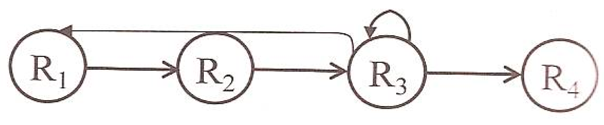
• R₁: Retrieve the most suitable past case to the new problem.
• R₂: Reuse the information of the retrieved case to solve the new problem.
• R₃: Revise the solution.
• R₄: Retain the part of the solution that could be useful for future problems.

Steps R₁, R₂ and R₃ are not linear, characterized by a backward–forward flow. A simple flow diagram of the CBR process is presented in Figure 6:

More information and a detailed functional diagram illustrating the four steps of the CBR process are presented in [42].

Example 4.

Consider a couple of CBR systems with a collection of 105 and 90 past cases, respectively. The designers have supplied both systems with a mechanism evaluating the degree of success of the past cases for solving new analogous problems.

Table 3. Assessment of the past cases of the CBR systems.

First system
Steps	F	D	C	B	A
R1	0	0	51	24	30
R2	18	18	48	21	0
R3	36	30	39	0	0
Second system
Steps	F	D	C	B	A
R1	0	18	45	27	0
R2	18	24	48	0	0
R3	36	27	27	0	0

depicts the performance of the past cases in the three first steps of the CBR process.

Here, we compare the mean performance of the two systems by applying both methods with TFNs and GNs.

(i) Use of TFNs: The data in Table 3 show that in Step R₁ we have for the first system 51 TFNs equal to C(60, 67, 74), 24 TFNs equal to B(75, 79.5, 85) and 30 TFNs equal to A(85, 92.5, 100). The calculation of the mean value of those TFNs gives that R₁ = $\frac{1}{105}$(51C + 24B + 30A) = $\frac{1}{105}$ [(3060, 3417, 3774) + (1800, 1908, 2016) + (2550, 2775, 3000) = $\frac{1}{105}$ (7410, 8100, 8790) ≈ (70.57, 77.14, 83.71).

Therefore, from Equation (15), one gets that X(R₁) = 77.14, which shows that the first system demonstrates a very good (B) performance at Step R1.

In the same way, one calculates for the first system the mean values R₂ = $\frac{1}{105}$ (18F + 18D+ 48C + 21B) ≈ (51, 60.07, 69.14) with X(R₂) = 60.07 and R₃ = $\frac{1}{105}$ (36F + 30D + 39C) ≈ (36.57, 48.86, 61.14) with X(R₂) = 48.86, thus obtaining the analogous conclusions for the system’s performance at Steps R₂ and R₃ of the CBR process.

The overall system’s performance can be assessed by the mean value R = $\frac{1}{3}$ (R₁ + R₂ + R₃) ≈ (52.71, 62.02, 71.33). Since X(R) = 62.02, the system demonstrates a good (C) mean performance.

A similar argument gives for the second system the values R₁ = (62.5, 68.25, 74), R₂ ≈ (45.33, 55.17, 65), R₃ = (33, 46.25, 59.5) and R ≈ (46.94, 56.56, 66.17). Therefore, analogous conclusions can be obtained for its mean performance at each step of the CBR process and for its overall mean performance, which is characterized as fair (D).

(ii) Use of GNs: Here, in Step R₁, we have 51 GNs equal to C ∈ [60, 74], 24 GNs equal to B ∈ [75, 84] and 30 GNs equal to A ∈ [85, 100]. The mean value of those GNs is R₁* = $\frac{1}{105}$ (51C + 24B + 30A) ∈ [70.57, 83.71]. Therefore, W(R₁*) = $\frac{70.57+83.71}{2}$= 77.14, etc.

Remarks 4.

(i)

As we show in the previous section, the use of GNs provides in general the same assessment outcomes with the use of TFNs. However, observe that, to obtain the mean value M* ∈ [m₁, m₂], one needs to calculate two components only, in contrast to the mean value M (a, b, c) where the calculation of three components is needed. Consequently, the method with GNs reduces the required computational burden.

(ii)

Another promising area for applying the above assessment methods is the fuzzy control systems (e.g., see [43], [44] (Paragraph 5.3), [45]). Traditional controllers, often implemented as PID (proportional–integral–derivative) controllers, are based on mathematical models in which the control system is described using one or more differential equations that define the system response to its inputs. They are the products of decades of development and theoretical analysis and are highly effective in general. However, in certain cases, the mathematical model of the control process may not exist, or may be too “expensive” in terms of computer processing power and memory. In such cases, a system based on empirical rules may be more effective.

Fuzzy controllers consist of input, processing and output stages. The input stage maps sensors, switches and other inputs to the appropriate membership functions (usually triangular, although trapezoidal and bell curves are also used) and truth values. The processing stage is based on a collection of logic rules in the form of IF–THEN statements. A result is generated from each rule and all these results are properly combined. For example, such a rule for a thermostat is “IF the temperature is low, THEN the heater is high”. Typical fuzzy controllers have dozens of rules. Finally, the output stage converts the combined result back into a specific control output value. In many cases, fuzzy control can be used to improve existing traditional control systems by adding an extra layer of intelligence to the current control method.

Example 5.

Six different trainers ranked with scores from 0 to 100 the performance of five athletes as follows: A₁ (Athlete 1): 43, 48, 49, 49, 50, and 52; A₂: 81, 83, 85, 88, 91, and 95; A₃: 76, 82, 89, 95, 95, and 98; A₄: 86, 86, 87, 87, 87, and 88; and A₅: 35, 40, 44, 52, 59, and 62.

The mean value of the 6 × 5 = 30 given numerical scores is approximately equal to 72.07, demonstrating a good (C) mean performance of the athletes. For reasons of comparison of the two methods, the system’s mean performance is also calculated using GNs.

The given numerical scores provide 14 GNs equal to A, 4 equal to B, 1 equal to C, 4 equal to D and 7 equal to F. Their mean value is M* = $\frac{1}{30}$(14A + 4B + C + 4D + 7F) ∈ [60.33, 79.63]. Therefore, Equation (18) gives that W(M*) = 69.98, which shows that the five athletes demonstrate a good performance, but the exact score corresponding to their mean performance is the mean value 72.02 of the given numerical scores calculated in the traditional way.

In conclusion, the assessment methods using GNs and TFNs, although they give a satisfactory approximation of the system’s mean performance, are practically useful only when the individual performance is evaluated by qualitative grades and not by numerical scores, because, in this case, the calculation of the mean value of those grades in the traditional way is not possible.

7. Application of Fuzzy Relation Equations to Mathematical Modeling

7.1. Mathematical Modeling

Until the mid-1970s, Mathematical Modeling (MM) was mainly a tool in the hands of scientists and engineers for solving real world problems related to their disciplines (physics, industry, constructions, economics, etc.). However, the failure to introduce “new mathematics” in school education brought the attention of researchers and educators to problem-solving processes, and in particular to the process of MM and its applications. As a result, MM appears today as a dynamic tool for teaching and learning mathematics, because it connects mathematics with our everyday life, giving the possibility to students to understand its usefulness in practice and therefore increasing their interest in it [46].

The steps of the MM process involve:

• S₁: Analyze the given problem (understanding the statement and recognizing the restrictions and requirements imposed by the corresponding real system).
• S₂: Mathematize (formulation of the problem and construction of the mathematical model).
• S₃: Solve the model.
• S₄: Validate (control) the model, which is usually achieved by reproducing, through the model, the behavior of the real system under the conditions existing before the solution of the model and by comparing it to the existing from the previous “history” of the real system, i.e., data. In cases of systems having no past history, an extra simulation model could be used for the validation of the mathematical model.
• S₅: Interpret the final mathematical results and implement them in the real system to give the “answer” to the real-world problem.

7.2. Fuzzy Relation Equations

Fuzzy Relation Equations (FREs) are associated with the composition of Fuzzy Binary Relations (FBRs). A FBR is defined as follows:

Definition 1.

Let X and Y be two crisp sets. Then, a FBR R(X, Y) is a FS on the Cartesian product X × Y of the form: R(X, Y) = {(r, mR(r): r = (x, y) ∈ X × Y}, where mR: X × Y → [0, 1] is the corresponding membership function. When X = {x₁,………, x_n} and Y = {y₁,……, y_m}, a FBR R(X, Y) can be represented by a n X m matrix R = [r_ij], where r_ij = m_R (x_i, y_j), with i = 1,…, n and j = 1,…, m. The matrix R is called the membership matrix of the FBR R(X, Y).

The basic ideas of fuzzy relations, which were introduced by Zadeh [47] and further investigated by other researchers, are extensively covered in the book [48].

Definition 2.

Consider two FBR P(X, Y) and Q(Y, Z) with a common set Y. Then, the standard composition of these relations, denoted by P(X, Y) ○ Q(Y, Z) produces a FBR R(X, Z) with membership function m_R defined by:

$${\mathrm{m}}_{\mathrm{R}}({\mathrm{x}}_{\mathrm{i}},{\mathrm{z}}_{\mathrm{j}})=\underset{y\in Y}{\max }\min [{\mathrm{m}}_{\mathrm{P}}({\mathrm{x}}_{\mathrm{i}},\mathrm{y}),{\mathrm{m}}_{\mathrm{Q}}(\mathrm{y},{\mathrm{z}}_{\mathrm{j}})],\mathrm{i}=1,\dots ,\mathrm{n},\mathrm{j}=1,\dots ,\mathrm{m}.$$

(19)

This composition is usually referred to as max-min composition. Compositions of FBR are conveniently performed in terms of their membership matrices. In fact, if P = [p_ik] and Q = [q_kj] are the membership matrices of the FBRs P(X, Y) and Q(Y, Z)m respectively, then by Equation (19)m we get that the membership matrix of R(X, Y) = P(X, Y) ○ Q(Y, Z) is the matrix R = [r_ij], with

$${\mathrm{r}}_{\mathrm{ij}}=\underset{k}{\max }\min ({\mathrm{p}}_{\mathrm{ik}},{\mathrm{q}}_{\mathrm{kj}}).$$

(20)

Note that the same elements of P and Q are used in the calculation of m_R as would be used in the regular multiplication of matrices, but the product and sum operations are here replaced with the min and max operations, respectively.

Definition 3.

Consider the FBRs P(X, Y), Q(Y, Z) and R(X, Z), defined on the sets X = {x_i: i ∈ Nn}, Y = {y_j: j ∈ Nm }, Z = {z_k: k ∈ Ns}, where Nt = {1,2,…,t}, for t = n, m, k, and let P = [p_ij], Q = [q_jk] and R = [r_ik] be the membership matrices of P(X, Y), Q(Y, Z) and R(X, Z), respectively. Assume that the above three relations constrain each other in such a way that P ○ Q = R, where ○ denotes the max-min composition. This means that, for each i in Nn and each k in Ns,

$${\mathrm{r}}_{\mathrm{ik}}=\underset{j\in J}{\max }\min ({\mathrm{p}}_{\mathrm{ij}},{\mathrm{q}}_{\mathrm{jk}}).$$

(21)

Therefore, the matrix equation P ○ Q = R encompasses nXs simultaneous equations of the form of Equation (21). When two of the components in Equation (21) are given and one is unknown, these equations are referred as FRE. The notion of FRE was first proposed by Sanchez [49] and later further investigated by other researchers (e.g., [50,51,52]).

7.3. A Study of MM Skills Using FRE

Let us consider the crisp sets X = {M}, Y = {A, B, C, D, F} and Z = {S₁, S₂, S₃, S₄}, where M denotes the imaginary notion of the average student of a class; A, B, C, D, and F are the linguistic grades used for the assessment of the student performance; and S₁, S₂, S₃, and S₄ are the steps of the MM process. Without loss of generality, the validation (S₄) and the implementation (S₅) of the model, which are usually considered as two different steps, have been joined here in one step (S₄) to make simpler the development of our assessment method.

Let n be the total number of students of a class and let n_i be the numbers of students of the class who obtained the grade i assessing their performance, i ∈ Y. Then, one can represent the average student of the class as a FS on Y in the form M = {(i,$\frac{{\mathrm{n}}_{\mathrm{i}}}{\mathrm{n}}$): i ∈ Y}.

The FS M induces a FBR P(X, Y) with membership matrix P = [$\frac{n_A}{n}$, $\frac{n_B}{n}$, $\frac{n_B}{n}$, $\frac{n_C}{n}$, $\frac{n_F}{n}$].

In an analogous way, the average student of a class can be represented as a FS on Z in the form M′ = {(j, m(j): j ∈ Z}, where m: Z → [0, 1] is the corresponding membership function. In this case, the FS M′ induces a FBR R(X, Z) with membership matrix R = [m(S₁) m(S₂) m(S₃) m(S₄)].

We consider also the FBR Q(Y, Z) with membership matrix the 5 × 4 matrix Q = [q_ij], where qij = m_Q(i, j) with i ∈ Y and j ∈ Z and the FRE encompassed by the matrix equation P ○ Q = R. When the matrix Q is fixed and the row-matrix P is known, then the above equation always has a unique solution with respect to R, which enables the representation of the average student of a class as a fuzzy set on the set of the steps of the MM process. This is useful for the instructor for designing his/her future teaching plans. On the contrary, when the matrices Q and R are known, then the equation P ○ Q = R may have no solution or it may have more than one solutions with respect to P, which makes the corresponding situation more complicated.

Example 6.

The following experiment took place at the Graduate Technological Educational Institute of Western Greece, in the city of Patras, when I was teaching a group of 60 students of the School of Technological Applications (future engineers) the use of the derivative for the maximization and minimization of a function. A written test was performed after the end of the teaching process involving two mathematical modeling problems about the construction of a channel to run water and of a cylindrical tower (see the second section of [46]). The results of the test are depicted in

Table 4. Student performance.

Grade	No. of Students
A	20
B	15
C	7
D	10
F	8
Total	60

.

Therefore, the average student M of the class can be represented as a fuzzy set on Y = {A, B, C, D, F} by M = {(A,$\frac{20}{60}$), (B, $\frac{15}{60}$), (C, $\frac{7}{60}$), (D, $\frac{10}{60}$), (F, $\frac{8}{60}$)} ≈ {(A, 0.33), (B, 0.25), (C, 0.12), (D, 0.17), (F, 0.13)}. Thus, M induces a FBR P(X, Y), where X = {M}, with membership matrix P = [0.33 0.25 0.12 0.17 0.13].

In addition, using statistical data of the last five academic years concerning the MM skills of the students of the School of Technological Applications, we fixed the membership matrix Q of the binary fuzzy relation Q(Y, Z), where Z = {S₁, S₂, S₃, S₄}, in the form:

$$\begin{array}{cc}& \begin{array}{cccc}{\mathrm{S}}_1& {\mathrm{S}}_2& {\mathrm{S}}_3& {\mathrm{S}}_4\end{array}\\ \begin{array}{c}\mathrm{A}\\ \mathrm{B}\\ \mathrm{C}\\ \mathrm{D}\\ \mathrm{F}\end{array}& \left(\begin{array}{cccc}0.7& 0.5& 0.3& 0\\ 0.4& 0.6& 0.3& 0.1\\ 0.2& 0.7& 0.6& 0.2\\ 0.1& 0.5& 0.7& 0.5\\ 0& 0.7& 0.5& 0.8\end{array}\right)\end{array}$$

The statistical data were collected by the instructor who was inspecting the student reactions during the solution of several MM problems in the classroom.

Next, using the max-min composition of FBR, one finds that the membership matrix of R(X, Z) = P(X, Y) ○ Q (Y, Z) is equal to R = P ○ Q = [0.33 0.33 0.3 0.17]. Therefore, the average student of the class can be expressed as a fuzzy set on Z by M = {(S₁, 0.33), (S₂, 0.33), (S₃, 0.3), (S₄, 0.17)}.

The conclusions obtained from the above expression of M are the following:

• Only $\frac{1}{3}$ of the students of the class were ready to use contents of their memory (background knowledge, etc.) to facilitate the solution of the given problems.
• All the above students were able to design the model and almost all of them were able to execute the solutions of the given problems.
• On the contrary, half of the above students could not check the correctness of the solutions found and therefore implement correctly the mathematical results to the real system.

The first conclusion was not surprising, since the majority of the students have the wrong habit to start studying the material of their courses the last month before the final exams. On the other hand, the second conclusion shows that the instructor’s teaching procedure was successful, enabling the diligent students to plan and execute successfully the solutions of the given problems. Finally, the last conclusion is explained by the fact that students, when solving MM problems, frequently omit to check if their solutions are compatible to the restrictions imposed by the real system. Therefore, the instructor should emphasize during his/her lectures that the last two steps of the MM process (validation and implementation) are not a formality, but have their own importance for preventing several mistakes.

Let us now consider the case where the membership matrices Q and R are known and we want to determine the matrix P representing the average student of the class as a fuzzy set on Y. This is a complicated case because we may have more than one solution or no solution at all. The following two examples illustrate this situation.

Example 7.

Consider the membership matrices Q and R of the previous example and set P = [p₁ p₂ p₃ p₄ p₅]. Then, the matrix equation P o Q = R encompasses the following equations:

• max {min (p₁, 0.7), min (p₂, 0.4), min (p₃, 0.2), min (p₄, 0.1), (p₅, 0)}= 0.33
• max {min (p₁, 0.5), min (p₂, 0.6), min (p₃, 0.7), min (p₄, 0.5), min (p₅, 0.1)}= 0.33
• max {min (p₁, 0.3), min (p₂, 0.3), min (p₃, 0.6), min (p₄, 0.7), (p₅, 0.5)}= 0.3
• max {min (p₁, 0), min (p₂, 0.1), min (p₃, 0.2), min (p₄, 0.5), min (p₅, 0.8)}= 0.17

The first of the above equations is true if, and only if, p₁ = 0.33 or p₂ = 0.33, values that satisfy the second and third equations as well. In addition, the fourth equation is true if, and only if, p₃ = 0.17, p₄ = 0.17 or p₅ = 0.17. Therefore, any combination of values of p₁, p₂, p₃, p₄, and p₅ in [0, 1] such that p₁ = 0.33 or p₂ = 0.33 and p₃ = 0.17, p₄ = 0.17 or p₅ = 0.17 is a solution of P o Q = R.

Let S(Q, R) = {P: P ○ Q = R } be the set of all solutions of P o Q = R. Then, one can define a partial ordering on S(Q, R) by P ≤ P′ ⇔ p_i ≤ p′_i, ∀_ι = 1, 2, 3, 4, 5.

It is well established that, whenever S(Q, R) is a non-empty set, it always contains a unique maximum solution and it may contain several minimal solutions [49]. It is further known that S(Q, R) is fully characterized by the maximum and minimal solutions in the sense that all its other elements are between the maximal and each of the minimal solutions [49]. A method of determining the maximal and minimal solutions of P o Q = R with respect to P is developed in [52].

Example 8.

Let Q = [q_ij], i = 1, 2, 3, 4, 5 and j = 1, 2, 3, 4 be as in Example 2 and let R = [1 0.33 0.3 0.17]. Then, the first equation encompassed by the matrix equation P o Q = R is max {min (p₁ , 0.7), min (p₂, 0.4), min (p₃, 0.2), min (p₄, 0.1), and min (p₅, 0)}= 1. In this case, it is easy to observe that the above equation has no solution with respect to p₁, p₂, p₃, p₄, and p₅, therefore the matrix equation P o Q = R has no solution with respect to P. In general, writing R = {r₁ r₂ r₃ r₄}, it becomes evident that we have no solution if $\underset{\mathrm{j}}{\max }{\mathrm{q}}_{\mathrm{ij}}<{\mathrm{r}}_{\mathrm{i}}$.

8. Discussion and Conclusions

The enormous development of technology during the last years makes human life easier and more comfortable. However, the technological progress creates in parallel more and more complicated artificial systems, which are difficult to be managed by the traditional scientific methods. As a result, while 50–60 years ago probability theory used to be a unique tool in the hands of scientists for dealing with situations characterized by uncertainty and/or vagueness, today this is no loneger the rule. In fact, the introduction of FL and its generalizations (intuitionistic FS, neutrosophic sets, etc.) and of other relative theories (rough sets, soft sets, GS theory, etc.) provide new tools for dealing with such situations in real life, science and technology and enable the solution of problems with fuzzy or approximate data, which cannot be solved with traditional techniques of probability theory. The applications of FL and its relevant theories have been rapidly expanded nowadays, covering almost all sectors of human activities.

The objective of this review article is to present the author’s research on developing methods for the assessment of human–machine capacities under fuzzy conditions. Those methods include:

• The measurement of the corresponding fuzzy system’s probabilistic uncertainty (generalized Shannon’s entropy) or its total possibilistic uncertainty (the sum of strife and non-specificity) for evaluating its mean performance. However, this method can be applied for comparing the performance of two different systems with respect to a common activity only under the assumption that the uncertainty in those systems is the same before the activity (equivalent systems). Moreover, the method cannot provide an exact characterization of a system’s performance and it involves laborious calculations.
• The utilization of the COG defuzzification technique (rectangular fuzzy assessment model) for assessing a fuzzy system’s quality performance. This method, initiated by Subbotin et al. [31], is useful, due to its logical nature, when comparing the performance of two systems with equal values of the traditional GPA index. In this case, the GPA index could lead to conclusions that are not close to the reality. On the contrary, for different values of the GPA index, the two methods provide the same assessment outcomes.
• The use of TFNs as assessment tools, a method that is easy to apply in practice and gives an exact characterization of the system’s mean performance. That method is useful when qualitative grades and not numerical scores are used for the evaluation of the system’s performance, which makes impossible the calculation of the mean value of those grades in a traditional way. However, a disadvantage of the method is that its understanding requires knowledge of basic principles of FS theory, which is not always easy for non-specialists.
• The use of GNs, instead of TFNs, as assessment tools. These two methods are equivalent to each other, providing the same assessment outcomes. However, GNs can be easily defined with the help of closed real intervals, which makes the method more accessible to non-specialists. Moreover, the use of GNs reduces significantly the required computational burden.
• The application of FRE for assessing MM skills. This method enables the teacher to obtain useful conclusions about student progress and was applied by the author, with the proper modifications each time, to various other assessment situations (problem-solving, learning a subject matter, human and machine reasoning, etc.) [53,54,55].

The above models provide an innovative framework for further research on human–machine assessment. Our future plans involve improving and extending our fuzzy and grey assessment methods and applying the principles of FL and GS theory to other fields of human activity as well. Note that such efforts have already been started by the author on solving equations, systems of equations and linear programming problems with fuzzy or grey data, connected to real life applications [56,57,58,59].

References

1. Balley, K.D. Sociology and the New Systems Theory: Toward a Theoretical Synthesis; State of New York Press: New York, NY, USA, 1994. [Google Scholar]
2. Xu, K.; Tang, L.C.; Xie, M.; Ho, S.L.; Zhu, M.L. Fuzzy assessment of FMEA for engine systems. Reliab. Eng. Syst. Saf. 2002, 75, 17–29. [Google Scholar] [CrossRef]
3. Liu, L.; Lee, H.-M. Fuzzy assessment method on sampling survey analysis. Expert Syst. Appl. 2009, 36, 5955–5961. [Google Scholar]
4. Macwan, N.; Srinivas, S.P. A Linguistic Fuzzy Approach for Employee Evaluation. Int. J. Adv. Res. Comput. Sci. Softw. Eng. 2014, 1, 975–980. [Google Scholar]
5. Liu, R.-T.; Huang, W.-C. Fuzzy Assessment on Reservoir Water Quality. J. Mar. Sci. Technol. 2015, 23, 231–239. [Google Scholar]
6. Jevscek, M. Competencies assessment using fuzzy logic. J. Univers. Excell. 2016, 5, 187–202. [Google Scholar]
7. Korner, S. Laws of Thought. In Encyclopaedia of Philosophy; Mac Millan: New York, NY, USA, 1967; Volume 4, pp. 414–417. [Google Scholar]
8. Lejewski, C. Jan Lukasiewicz. Encycl. Philos. 1967, 5, 104–107. [Google Scholar]
9. Tarski, A. Encyclopaedia Brittanica. 2018. Available online: www.britannica.com/biography/Alfred-Tarski (accessed on 20 December 2018).
10. Zadeh, L.A. Outline of a new approach to the analysis of complex systems and decision processes. IEEE Trans. Syst. Man Cybern. 1973, 3, 28–44. [Google Scholar] [CrossRef]
11. Zadeh, L.A. Fuzzy Sets. Inf. Control 1965, 8, 338–353. [Google Scholar] [CrossRef]
12. Klir, G.J.; Folger, T.A. Fuzzy Sets, Uncertainty and Information; Prentice-Hall: London, UK, 1988. [Google Scholar]
13. Haack, S. Do we need fuzzy logic? Int. J. Man-Mach. Stud. 1979, 11, 437–445. [Google Scholar] [CrossRef]
14. Fox, J. Towards a reconciliation of fuzzy logic and standard logic. Int. J. Man Mach. Stud. 1981, 15, 213–220. [Google Scholar] [CrossRef]
15. Tah, J.H.M.; Carr, V. A proposal for construction project risk assessment using fuzzy logic. Constr. Manag. Econ. 2010, 18, 491–500. [Google Scholar] [CrossRef]
16. Collatta, M.; Pau, G.; Solerno, V.M.; Scata, G. A novel trust based algorithm for carpooling transportation systems. In Proceedings of the IEEE International Energy Conference and Exhibition, Florence, Italy, 9–12 September 2012. [Google Scholar]
17. Voskoglou, M.G. Finite Markov Chain and Fuzzy Logic Assessment Models: Emerging Research and Opportunities; Createspace.com–Amazon: Columbia, SC, USA, 2017. [Google Scholar]
18. Wu, C.; Liu, G.; Huang, G.; Liu, Q.; Guan, X. Ecological Vulnerability Assessment Based on Fuzzy Analytical Method and Analytic Hierarchy Process in Yellow River Delta. Int. J. Environ. Res. Public Health 2018, 15, 855. [Google Scholar] [CrossRef] [PubMed]
19. Nilashi, M.; Cavallaro, F.; Mardani, A.; Zavadskas, E.K.; Samad, S.; Ibrahim, O. Measuring Country Sustainability Performance Using Ensembles of Neuro-Fuzzy Technique. Sustainability 2018, 10, 2707. [Google Scholar] [CrossRef]
20. Atanassov, K.T. Intuitionistic Fuzzy Sets. Fuzzy Sets Syst. 1986, 20, 87–96. [Google Scholar] [CrossRef]
21. Smarandache, F. Neutrosophy/Neutrosophic Probability, Set, and Logic; Proquest: Ann Arbor, MI, USA, 1998. [Google Scholar]
22. Deng, J. Control Problems of Grey Systems. Syst. Control Lett. 1982, 1, 288–294. [Google Scholar]
23. Pawlak, Z. Rough Sets: Aspects of Reasoning about Data; Kluer Academic Publishers: Dordrecht, The Netherlands, 1991. [Google Scholar]
24. Molodtsov, D. Soft Set Theory–First Results. Comput. Math. Appl. 1999, 37, 19–31. [Google Scholar] [CrossRef]
25. Shannon, C.E. A mathematical theory of communications. Bell Syst. Tech. J. 1948, 27, 379–423, 623–656. [Google Scholar] [CrossRef]
26. Klir, G.J. Principles of Uncertainty: What are they? Why do we need them? Fuzzy Sets Syst. 1995, 74, 15–31. [Google Scholar] [CrossRef]
27. Shackle, G.L.S. Decision, Order and Time in Human Affairs; Cambridge University Press: Cambridge, UK, 1961. [Google Scholar]
28. Van Broekhoven, E.; De Baets, B. Fast and accurate centre of gravity defuzzification of fuzzy systems outputs defined on trapezoidal fuzzy partitions. Fuzzy Sets Syst. 2006, 157, 904–918. [Google Scholar] [CrossRef]
29. Voskoglou, M.G. An Application of Fuzzy Sets to the Process of Learning. Heuristics Didact. Exact Sci. 1999, 10, 9–13. [Google Scholar]
30. Voskoglou, M.G. Transition across Levels in the Process of Learning. Int. J. Model. Appl. 2009, 1, 37–44. [Google Scholar]
31. Subbotin, I.Y.; Badkoobehi, H.; Bilotckii, N.N. Application of fuzzy logic to learning assessment. Didact. Math. Probl. Investig. 2004, 22, 38–41. [Google Scholar]
32. Subbotin, I.Y. Trapezoidal Fuzzy Logic Model for Learning Assessment. arXiv, 2014; arXiv:1407.0823. [Google Scholar]
33. Zadeh, L.A. The Concept of a Linguistic Variable and its Application to Approximate Reasoning, Parts 1–3. Inf. Sci. 1975, 8, 9, 43–80, 199–249, and 301–357 . [Google Scholar] [CrossRef]
34. Sakawa, M. Fuzzy Sets and Interactive Multiobjective Optimization; Plenum Press: London, UK, 1993. [Google Scholar]
35. Kaufmann, A.; Gupta, M. Introduction to Fuzzy Arithmetic; Van Nostrand Reinhold Company: New York, NY, USA, 1991. [Google Scholar]
36. Voskoglou, M.G. Use of the Triangular Fuzzy Numbers for Student Assessment. Am. J. Appl. Math. Stat. 2015, 3, 146–150. [Google Scholar]
37. Voskoglou, M.G. Assessment of Human Skills Using Trapezoidal Fuzzy Numbers. Am. J. Appl. Math. Stat. 2015, 5, 111–116. [Google Scholar]
38. Deng, J. Introduction to Grey System Theory. J. Grey Syst. 1989, 1, 1–24. [Google Scholar]
39. Moore, R.A.; Kearfort, R.B.; Clood, M.J. Introduction to Interval Analysis, 2nd ed.; SIAM: Philadelphia, PA, USA, 1995. [Google Scholar]
40. Liu, S.F.; Lin, Y. (Eds.) Advances in Grey System Research; Springer: Berlin/Heidelberg, Germany, 2010. [Google Scholar]
41. Voskoglou, M.G.; Theodorou, Y. Application of Grey Numbers to Assessment Processes. Int. J. Appl. Fuzzy Sets Artif. Intell. 2017, 7, 59–72. [Google Scholar]
42. Voskoglou, M.G.; Salem, A.-B.M. Analogy-Based and Case-Based Reasoning: Two Sides of the Same Coin. Int. J. Appl. Fuzzy Sets Artif. Intell. 2014, 4, 7–18. [Google Scholar]
43. Reznik, L. Fuzzy Controllers; Newnes: Oxford, UK, 1997. [Google Scholar]
44. Theodorou, Y.A. Introduction to Fuzzy Logic; Tziolas Editions: Thessaloniki, Greece, 2010. (In Greek) [Google Scholar]
45. Wikipedia. Fuzzy Control System. March 2012. Available online: http://en.wikipedia.org/wiki/Fuzzy_control_system (accessed on 20 December 2018).
46. Voskoglou, M.G. Mathematical modelling as a teaching method of mathematics. J. Res. Innov. Teach. (Natl. Univ. CA) 2015, 8, 35–50. [Google Scholar]
47. Zadeh, L.A. Similarity relations and fuzzy orderings. Inf. Sci. 1971, 3, 177–200. [Google Scholar] [CrossRef]
48. Kaufmann, A. Introduction to the Theory of Fuzzy Subsets; Academic Press: New York, NY, USA, 1975. [Google Scholar]
49. Sanchez, E. Resolution of Composite Fuzzy Relation Equations. Inf. Control 1976, 30, 38–43. [Google Scholar] [CrossRef]
50. Prevot, M. Algorithm for the solution of fuzzy relations. Fuzzy Sets Syst. 1981, 5, 319–322. [Google Scholar] [CrossRef]
51. Czogala, E.; Drewniak, J.; Pedryz, W. Fuzzy relation equations on a finite set. Fuzzy Sets Syst. 1982, 7, 89–101. [Google Scholar] [CrossRef]
52. Higashi, M.; Klir, G.J. Resolution of finite fuzzy relation equations. Fuzzy Sets Syst. 1984, 13, 65–82. [Google Scholar] [CrossRef]
53. Voskoglou, M.G. A Study of Student Learning Skills Using Fuzzy Relation Equations. Egypt. Comput. Sci. J. 2018, 42, 80–87. [Google Scholar]
54. Voskoglou, M.G. Application of Fuzzy Relation Equations to Assessment of Analogical Problem Solving Skills. J. Phys. Math. Educ. 2018, 15, 122–127. [Google Scholar] [CrossRef]
55. Voskoglou, M.G. Application of Fuzzy Relation Equations Student Assessment. Am. J. Appl. Math. Stat. 2018, 6, 167–171. [Google Scholar] [CrossRef]
56. Voskoglou, M.G. Solving Systems of Equations with Grey Data. Int. J. Appl. Fuzzy Sets Artif. Intell. 2018, 8, 103–111. [Google Scholar]
57. Voskoglou, M.G. Solving Linear Programming Problems with Grey Data. Orient. J. Phys. Sci. 2018, 3, 17–23. [Google Scholar]
58. Voskoglou, M.G. Fuzzy Linear Programming. Egypt. J. Comput. Sci. 2018, 42, 1–14. [Google Scholar]
59. Voskoglou, M.G. Systems of Equations with Fuzzy Coefficients. J. Phys. Sci. 2018, 23, 77–88. [Google Scholar]
Figure 1. Plato (left) and Aristotle in a Raphael’s fresco (1509).
Mathematics 07 00230 g001
Figure 2. L.A. Zadeh (1921–2017).
Mathematics 07 00230 g002
Figure 3. The graph of the membership function.
Mathematics 07 00230 g003
Figure 4. The triangle where the COG lies.
Mathematics 07 00230 g004
Figure 5. Graph and COG of the TFN (a, b, c).
Mathematics 07 00230 g005
Figure 6. A simplified flow-chart of the CBR process.
Mathematics 07 00230 g006