Cross Diffusion Induced Turing Patterns in a Tritrophic Food Chain Model with Crowley-Martin Functional Response

Abstract

Diffusion has long been known to induce pattern formation in predator prey systems. For certain prey-predator interaction systems, self diffusion conditions ceases to induce patterns, i.e., a non-constant positive solution does not exist, as seen from the literature. We investigate the effect of cross diffusion on the pattern formation in a tritrophic food chain model. In the formulated model, the prey interacts with the mid level predator in accordance with Holling Type II functional response and the mid and top level predator interact via Crowley-Martin functional response. We prove that the stationary uniform solution of the system is stable in the presence of diffusion when cross diffusion is absent. However, this solution is unstable in the presence of both self diffusion and cross diffusion. Using a priori analysis, we show the existence of a inhomogeneous steady state. We prove that no non-constant positive solution exists in the presence of diffusion under certain conditions, i.e., no pattern formation occurs. However, pattern formation is induced by cross diffusion because of the existence of non-constant positive solution, which is proven analytically as well as numerically. We performed extensive numerical simulations to understand Turing pattern formation for different values of self and cross diffusivity coefficients of the top level predator to validate our results. We obtained a wide range of Turing patterns induced by cross diffusion in the top population, including floral, labyrinth, hot spots, pentagonal and hexagonal Turing patterns.

1. Introduction

The two primary objectives of studying systems ecology are to get an understanding of the dynamics of the ecological systems and the nature of the forces, which determine the community structure. Earlier, the classical ecological models focused on two species interactions. Continuous time models of two interacting species have been studied extensively in the literature (see [1] and references therein). Mathematically, only two basic patterns are exhibited in these models—approach to a steady state or to a limit cycle [2]—but the ecological models of nature exhibit very complex dynamical behavior. Price et al. [3] proposed that community behavior must be based on three or more trophic levels. Three species continuous time models have observed more complex dynamical behavior [4,5,6,7]. All these studies depend upon the classical types of functional responses, which include Holling Types I, II and III and Holling-Tanner ratio dependent functional response.

The Crowley-Martin [8] functional response is one of the predator dependent functional responses, i.e., the functional response is function of both prey and predator abundance because of predator interference. The basic assumption behind the formulation of Crowley-Martin functional response is that there is a decrease in predator feeding rate because of high predator density even if there is a high prey density. Hence, the effect of predator interference on the feeding rate is important, even when an individual predator is handling or searching for a prey at a given instant of time. Here, v and r are population density of prey and predator, respectively. The parameters $w_2,d,b$ are positive parameters that describe the effects of capture rate, handling time and magnitude of interference among predators on the feeding rate, respectively. The per capita rate in this formulation is given by:

$${\displaystyle f(v,r)={\displaystyle \frac{w_{2}v}{1+dv+br+bdvr}}.}$$

The Crowley-Martin functional response is used for datasets that indicate an asymptotic feeding rate that is affected by predator density. A continuous time model to analyze the dynamics of a three species food chain with Crowley-Martin functional response was studied by Upadhyay et al. [9]. The model system in [9] is based on the assumption that the species under consideration are spatially homogeneously distributed; however, in nature, the species distribution is always inhomogeneous. Therefore, to model a realistic food chain scenario, reaction diffusion mechanism should be considered, as employed in [10,11,12]. A qualitative analysis of a two species model with Crowley-Martin functional response and diffusion is carried out in [13]. In the above model, the movement of a species is determined solely by their own characteristics, i.e., the movements of the species in these models are physically affected by the population pressures due to the mutual interference among the individuals of the same species. Therefore, such models take into account only the self diffusion of the species in concern. However, in the case of prey-predator interacting systems, the movement of one species may affect the movement or motility of the other. The above models fail to describe such situation, which is more realistic. In many systems, the predators develop migratory strategies to take advantage over the prey. In the case of a three species prey-predator model, such a migratory behavior depends on the concentration of both predators (i.e., the mid level predator and the top level predator). This leads to cross diffusive system, in addition to each species natural tendency to diffuse i.e., self diffusion; such models are studied in [14,15,16,17,18]. The cross diffusive coefficient may have positive or negative values. The positive cross diffusivity coefficient represents that one species tends to move in the direction of lower concentration of another species. The negative cross diffusion term represents that the population flux of one species is in the direction of higher concentration of the other species.

In the present paper, we consider a tritrophic food chain model in which the species interact via Crowley-Martin and Holling type II functional response at different levels. We introduce a nonlinear cross diffusion among top level and mid level predators. The objective is to understand the effect of both types of diffusion self and cross on the stability of the system. An analytic approach is adopted to understand the formation of inhomogeneous steady state solutions. Numerical simulation depicting spatial pattern formation was performed for a wide range of parameters to understand the predation behavior due to the effect of cross and self diffusion.

In Section 2, we formulate the temporal model using various assumptions and spatially extend it to formulate a nonlinear reaction diffusion system and with cross diffusivity (a strongly coupled parabolic system). In Section 3, we perform a linear stability analysis of the temporal model and obtain the conditions under which the stationary uniform solution is locally asymptotically stable. In Section 4, we provide analytical proof of stability of the stationary uniform solution in the presence of diffusion and in the absence of cross diffusion but unstable in the presence of cross diffusion. In Section 5, we provide an analytical proof of the existence of inhomogeneous steady states. Section 6 deals with the numerical simulation of the cross diffusive system and explains Turing pattern formation for different values of cross diffusive and self diffusive coefficients of the top level predator.

2. Model System

We first consider a temporal model governing the dynamics of tritrophic food chain, consisting of Holling type-II and Crowley Martin type functional responses, defined by a system of differential equations [9]. Here, $U(T)$ is the population density of the lowest trophic level species (prey), $V(T)$ is the population density of the middle trophic level species (intermediate predator) and $R(T)$ is the population density of the highest trophic level species (top predator), at any time T. We made the following basic assumptions for formulation of the proposed model system.

Assumption 1.

The prey U grows with an intrinsic growth rate $a_1$, and has a carrying capacity of K in the absence of predator V. D is a measure of the extent to which the environment can provide protection to U and w is the maximum value which per capita reduction rate of U can attain. In addition, the mid level predator V predates on U in accordance with Holling Type II functional response, ${\displaystyle {\displaystyle \frac{wUV}{U+D}}}$. Therefore, considering the above assumptions, we formulate the first equation of the model system as:

$${\displaystyle \frac{dU}{dT}}=a_{1}U\left(1-{\displaystyle \frac{U}{K}}\right)-{\displaystyle \frac{wUV}{U+D}}$$

(1)

Assumption 2.

The intermediate or mid level predator V has a natural death rate of $a_2$. $w_1$ describes the maximum value which per capita reduction rate of V can attain, $D_1$ is similar to D of U and p represents the internal competition coefficient among the members of V. The predation of V over U is governed by Holling Type II functional response. The top level predator R predates on V in accordance with Crowley-Martin functional response. The constants $w_2$, b and d are the saturating Crowley-Martin type functional response parameters, where $w_2$ describes capture rate effect, b represents handling time of prey and d is the magnitude of interference among predators. The second equation of the model system is given as:

$${\displaystyle \frac{dV}{dT}}=-a_{2}V-p{V}^2+{\displaystyle \frac{w_{1}UV}{U+D_1}}-{\displaystyle \frac{w_{2}VR}{1+dV+bR+bdVR}}$$

(2)

Assumption 3.

The top level predator R dies at a natural death rate of c. As the predating behavior of R over V is described by the Crowley-Martin functional response. $w_3$ is the saturating Crowley-Martin type functional response parameter similar to $w_2$. The third equation of the model system takes the following form:

$${\displaystyle \frac{dR}{dT}}=-cR+{\displaystyle \frac{w_{3}VR}{1+dV+bR+bdVR}}$$

(3)

All parameters described above take only positive values and the model system is a three species food chain model involving a hybrid type of prey dependent and predator dependent functional response. Therefore, using the above assumptions, the model system takes the following form:

$$\begin{array}{c}\hfill \begin{array}{cc}\hfill {\displaystyle \frac{dU}{dT}}& =a_{1}U\left(1-{\displaystyle \frac{U}{K}}\right)-{\displaystyle \frac{wUV}{U+D}}\hfill \\ \hfill {\displaystyle \frac{dV}{dT}}& =-a_{2}V-p{V}^2+{\displaystyle \frac{w_{1}UV}{U+D_1}}-{\displaystyle \frac{w_{2}VR}{1+dV+bR+bdVR}}\hfill \\ \hfill {\displaystyle \frac{dR}{dT}}& =-cR+{\displaystyle \frac{w_{3}VR}{1+dV+bR+bdVR}}\hfill \end{array}\end{array}$$

(4)

The model system described by Equation (4) consists of thirteen parameters, which makes the analysis quite cumbersome, therefore the number of parameters are reduced by rescaling the model system. The model is rescaled, using the following new variables and parameters:

$$\begin{array}{c}t=a_{1}T,u={\displaystyle \frac{U}{K}},v={\displaystyle \frac{wV}{a_{1}K}},r={\displaystyle \frac{w{w}_{2}R}{a_1^{2}dK}},w_4={\displaystyle \frac{D}{K}},w_5={\displaystyle \frac{a_2}{a_1}},w_6={\displaystyle \frac{w_1}{a_1}},w_7={\displaystyle \frac{D_1}{K}},\hfill \\ w_8={\displaystyle \frac{a_{1}b}{w_2}},w_9={\displaystyle \frac{a_1^{2}bdK}{w{w}_2}},w_{10}={\displaystyle \frac{w}{a_{1}dK}},w_{11}={\displaystyle \frac{c}{a_1}},w_{12}={\displaystyle \frac{w_3}{a_{1}d}},e={\displaystyle \frac{pw}{a_1^{2}K}}\hfill \end{array}$$

(5)

The rescaled system is as follows:

$$\begin{array}{c}\hfill \begin{array}{cc}\hfill {\displaystyle \frac{du}{dt}}& =u\left(1-u-{\displaystyle \frac{v}{u+w_4}}\right)\hfill \\ \hfill {\displaystyle \frac{dv}{dt}}& =v\left(-w_5+{\displaystyle \frac{w_{6}u}{u+w_7}}-ev-{\displaystyle \frac{r}{v+\left(w_8+w_{9}v\right)r+w_{10}}}\right)\hfill \\ \hfill {\displaystyle \frac{dr}{dt}}& =r\left(-w_{11}+{\displaystyle \frac{w_{12}v}{v+\left(w_8+w_{9}v\right)r+w_{10}}}\right)\hfill \end{array}\end{array}$$

(6)

The model system proposed in Equation (4) and the rescaled form of the model given in Equation (6) are based on the assumption that the species under consideration are homogeneously distributed but in nature the species distribution is always inhomogeneous. Therefore, to model a realistic food chain scenario, we consider the model system with diffusion. Consider the spatially explicit three species predator prey food chain model system. At any location $(x,y)$ and time t, the interaction of three species populations $u(x,y,t)$, $v(x,y,t)$ and $r(x,y,t)$ can be modeled with the reaction diffusion equations given in Equation (7). Here, $\mathsf{\Delta }$ denotes two dimensional Laplacian operator given by $\left({\displaystyle \mathsf{\Delta }\equiv {\displaystyle \frac{{\partial }^2}{\partial x^2}}+{\displaystyle \frac{{\partial }^2}{\partial y^2}}}\right)$, where, $x,y\in \mathsf{\Omega }$ and $t>0$. $\mathsf{\Omega }$ is a bounded domain in ${\mathbb{R}}^2$ with a smooth boundary $\partial \mathsf{\Omega }$.

$$\begin{array}{c}\hfill \begin{array}{c}{\displaystyle \frac{\partial u}{\partial t}}-d_1\mathsf{\Delta }u=u\left(1-u-{\displaystyle \frac{v}{u+w_4}}\right)\hfill \\ {\displaystyle \frac{\partial v}{\partial t}}-d_2\mathsf{\Delta }v=v\left(-w_5+{\displaystyle \frac{w_{6}u}{u+w_7}}-ev-{\displaystyle \frac{r}{v+\left(w_8+w_{9}v\right)r+w_{10}}}\right)\hfill \\ {\displaystyle \frac{\partial r}{\partial t}}-d_3\mathsf{\Delta }r=r\left(-w_{11}+{\displaystyle \frac{w_{12}v}{v+\left(w_8+w_{9}v\right)r+w_{10}}}\right)\hfill \\ {\displaystyle \frac{\partial u}{\partial n}}={\displaystyle \frac{\partial v}{\partial n}}={\displaystyle \frac{\partial r}{\partial n}}=0.\hfill \end{array}\end{array}$$

(7)

The boundary conditions ${\displaystyle {\displaystyle \frac{\partial u}{\partial n}}={\displaystyle \frac{\partial v}{\partial n}}={\displaystyle \frac{\partial r}{\partial n}}=0}$ are directional derivative normal to the boundary and n is the outward normal to $\mathsf{\Omega }$.

In the above system, the movement of a species is determined solely by their own characteristics, i.e., the movements of the species can be physically affected by the population pressures due to the mutual interference between the individuals of the same species. Therefore, we refer to the constants $d_1$, $d_2$ and $d_3$ as the self diffusion rates of species u, v and r, respectively. However, in the case of a prey-predator interacting system, the movement of one species may affect the movement or motility of the other. Hence, the above model cannot be used to describe such a situation. There are chances of development of migratory strategies among the predators to take advantage over the prey. This behavior can be described by taking into account the effect of cross diffusion. Along with the self tendency to move, i.e., self diffusion, the species also migrate or move under the influence of other. Such behavior takes into account concentration of both predators—the mid and the top level predators—constituting a cross diffusive system. The coefficient of cross diffusion may be positive or negative. The positive cross diffusion coefficient represents that one species tends to move in the direction of lower concentration of another species. The negative cross diffusion term represents that the population flux of one species is in the direction of higher concentration of the other. Therefore, we propose the interaction of the above three species population model with cross diffusion as follows:

$$\begin{array}{c}\hfill \begin{array}{c}{\displaystyle \frac{\partial u}{\partial t}}-d_1\mathsf{\Delta }u=u\left(1-u-{\displaystyle \frac{v}{u+w_4}}\right)\hfill \\ {\displaystyle \frac{\partial v}{\partial t}}-d_2\mathsf{\Delta }v=v\left(-w_5+{\displaystyle \frac{w_{6}u}{u+w_7}}-ev-{\displaystyle \frac{r}{v+\left(w_8+w_{9}v\right)r+w_{10}}}\right)\hfill \\ {\displaystyle \frac{\partial r}{\partial t}}-d_3\mathsf{\Delta }\left(r+d_{4}vr\right)=r\left(-w_{11}+{\displaystyle \frac{w_{12}v}{v+\left(w_8+w_{9}v\right)r+w_{10}}}\right)\hfill \\ {\displaystyle \frac{\partial u}{\partial n}}={\displaystyle \frac{\partial v}{\partial n}}={\displaystyle \frac{\partial r}{\partial n}}=0.\hfill \end{array}\end{array}$$

(8)

where $\mathsf{\Delta }$ denotes two dimensional Laplacian operator given by $\left({\displaystyle \mathsf{\Delta }\equiv {\displaystyle \frac{{\partial }^2}{\partial x^2}}+{\displaystyle \frac{{\partial }^2}{\partial y^2}}}\right)$, $(x,y)\in \mathsf{\Omega }$.

The nonlinear diffusion terms in the equation governing the dynamics of top level predator r implies that the direction of dispersion of top predator contains a self diffusion term by which it moves from a region of its higher concentration to a region of its lower concentration and a cross diffusive term. The top predator r diffuses with the flux

$$\mathbf{J}=-\nabla \left(d_{3}r+d_3{d}_{4}vr\right)=-d_3{d}_{4}r\nabla v-\left(d_3+d_3{d}_{4}v\right)\nabla r.$$

where the $-d_3{d}_4\nabla r<0$, the $-d_3{d}_{4}r\nabla v$ part of the flux $\mathbf{J}$ is directed towards the decreasing population density of mid level predator v. This is because, in certain prey-predator systems, several prey form a huge group to protect themselves from the attacking predators. In addition, as in the model system the predation of top predator is impossible, to extensively study the role of cross diffusion on the model system, we induce it at r, i.e., the top predator.

3. Linear Stability Analysis of Temporal Model

Under the assumption that the model system in Equation in Equation (6) has the unique positive stationary uniform solution, which we denote by ${\mathbf{u}}^{\ast }=(u^{\ast },v^{\ast },r^{\ast })$ (where ${\mathbf{u}}^{\ast }$ is a three coordinate vector), we derive the conditions under which it is locally asymptotically stable.

Theorem 1.

The positive equilibrium solution given by ${\mathbf{u}}^{\ast }=(u^{\ast },v^{\ast },r^{\ast })$ of the model system in Equation (6) is locally asymptotically stable if the parameters satisfy,

$${\displaystyle \frac{r^{\ast }{v}^{\ast }(1+w_9{r}^{\ast })}{{\left[v^{\ast }+\left(w_8+w_9{v}^{\ast }\right)r^{\ast }+w_{10}\right]}^2}}<eand{\displaystyle \frac{v^{\ast }}{{(u^{\ast }+w_4)}^2}}<1.$$

(9)

Proof. 

We consider the following notation given in Equation (10):

$$\mathbf{G}(\mathbf{u})=\left(\begin{array}{c}{G}_1(\mathbf{u})\\ G_2(\mathbf{u})\\ G_3(\mathbf{u})\end{array}\right)=\left(\begin{array}{c}\begin{array}{cc}\hfill u{g}_1(\mathbf{u})\cong & u\left(1-u-{\displaystyle \frac{v}{u+w_4}}\right)\hfill \\ \hfill v{g}_2(\mathbf{u})\cong & v\left(-w_5+{\displaystyle \frac{w_{6}u}{u+w_7}}-ev-{\displaystyle \frac{r}{v+\left(w_8+w_{9}v\right)r+w_{10}}}\right)\hfill \\ \hfill r{g}_3(\mathbf{u})\cong & r\left(-w_{11}+{\displaystyle \frac{w_{12}v}{v+\left(w_8+w_{9}v\right)r+w_{10}}}\right)\hfill \end{array}\end{array}\right)$$

(10)

Calculating ${\mathbf{G}}_{\mathbf{u}}({\mathbf{u}}^{\ast })$, and putting, ${\mathbf{G}}_{\mathbf{u}}({\mathbf{u}}^{\ast })=0$.

$${\mathbf{G}}_{\mathbf{u}}({\mathbf{u}}^{\ast })=\left(\begin{array}{ccc}{\displaystyle \frac{u^{\ast }{v}^{\ast }}{{(u^{\ast }+w_4)}^2}}-u^{\ast }& {\displaystyle \frac{-u^{\ast }}{u^{\ast }+w_4}}& 0\\ {\displaystyle \frac{w_6{w}_7{v}^{\ast }}{{(u^{\ast }+w_7)}^2}}& -e{v}^{\ast }+{\displaystyle \frac{r^{\ast }{v}^{\ast }(1+w_9{r}^{\ast })}{{\left[v^{\ast }+\left(w_8+w_9{v}^{\ast }\right)r^{\ast }+w_{10}\right]}^2}}& -{\displaystyle \frac{v^{\ast }(v^{\ast }+w_{10})}{{\left[v^{\ast }+\left(w_8+w_9{v}^{\ast }\right)r^{\ast }+w_{10}\right]}^2}}\\ 0& {\displaystyle \frac{r^{\ast }{w}_{12}(w_8{r}^{\ast }+w_{10})}{{\left[v^{\ast }+\left(w_8+w_9{v}^{\ast }\right)r^{\ast }+w_{10}\right]}^2}}& {\displaystyle \frac{-w_{12}{v}^{\ast }{r}^{\ast }(w_8+w_9{v}^{\ast })}{{\left[v^{\ast }+\left(w_8+w_9{v}^{\ast }\right)r^{\ast }+w_{10}\right]}^2}}\end{array}\right)$$

(11)

Here, $\rho (\lambda )$ denotes the characteristic polynomial of ${\mathbf{G}}_{\mathbf{u}}({\mathbf{u}}^{\ast })$ given by:

$$\rho (\lambda )={\lambda }^3+H_1{\lambda }^2+H_2\lambda +H_3$$

where

$$\begin{array}{cc}\hfill H_1=& {\displaystyle \frac{w_{12}{v}^{\ast }{r}^{\ast }\left(w_8+w_9{v}^{\ast }\right)}{{\left[v^{\ast }+\left(w_8+w_9{v}^{\ast }\right)r^{\ast }+w_{10}\right]}^2}}+v^{\ast }\left(e-{\displaystyle \frac{r^{\ast }{v}^{\ast }(1+w_9{r}^{\ast })}{{\left[v^{\ast }+\left(w_8+w_9{v}^{\ast }\right)r^{\ast }+w_{10}\right]}^2}}\right)+u^{\ast }\left(1-{\displaystyle \frac{v^{\ast }}{{(u^{\ast }+w_4)}^2}}\right)\hfill \end{array}$$

$$\begin{array}{cc}\hfill H_2=& u^{\ast }\left(1-{\displaystyle \frac{v^{\ast }}{{(u+w_4)}^2}}\right)\left\{{\displaystyle \frac{w_{12}{v}^{\ast }{r}^{\ast }(w_8+w_9{v}^{\ast })}{{\left[v^{\ast }+\left(w_8+w_9{v}^{\ast }\right)r^{\ast }+w_{10}\right]}^2}}+v^{\ast }\left(e-{\displaystyle \frac{r^{\ast }{v}^{\ast }(1+w_9{r}^{\ast })}{{\left[v^{\ast }+\left(w_8+w_9{v}^{\ast }\right)r^{\ast }+w_{10}\right]}^2}}\right)\right\}\hfill \\ & +{\displaystyle \frac{w_6{w}_7{u}^{\ast }{v}^{\ast }}{(u^{\ast }+w_4){(u^{\ast }+w_7)}^2}}+{\displaystyle \frac{v^{\ast }{r}^{\ast }{w}_{12}(v^{\ast }+w_{10})(w_8{r}^{\ast }+w_{10})}{{\left[v^{\ast }+\left(w_8+w_9{v}^{\ast }\right)r^{\ast }+w_{10}\right]}^2}}+{\displaystyle \frac{w_{12}{v}^{\ast 2}{r}^{\ast }(w_8+w_9)}{{\left[v^{\ast }+\left(w_8+w_9{v}^{\ast }\right)r^{\ast }+w_{10}\right]}^2}}\hfill \\ & \times \left(e-{\displaystyle \frac{r^{\ast }{v}^{\ast }(1+w_9{r}^{\ast })}{{\left[v^{\ast }+\left(w_8+w_9{v}^{\ast }\right)r^{\ast }+w_{10}\right]}^2}}\right)\hfill \end{array}$$

$$\begin{array}{cc}\hfill H_3=& {\displaystyle \frac{w_6{w}_7{u}^{\ast }{v}^{\ast 2}{r}^{\ast }(w_8+w_9{r}^{\ast })}{(u+w_4){(u+w_7)}^2{\left[v^{\ast }+\left(w_8+w_9{v}^{\ast }\right)r^{\ast }+w_{10}\right]}^2}}+\{{\displaystyle \frac{v^{\ast }{r}^{\ast }{w}_{12}(v^{\ast }+w_{10})(w_8{r}^{\ast }+w_{10})}{{\left[v^{\ast }+\left(w_8+w_9{v}^{\ast }\right)r^{\ast }+w_{10}\right]}^2}}\hfill \\ & +\left({\displaystyle \frac{w_{12}{v}^{\ast 2}{r}^{\ast }(w_8+w_9)}{{\left[v^{\ast }+\left(w_8+w_9{v}^{\ast }\right)r^{\ast }+w_{10}\right]}^2}}\right)\left(e-{\displaystyle \frac{r^{\ast }{v}^{\ast }(1+w_9{r}^{\ast })}{{\left[v^{\ast }+\left(w_8+w_9{v}^{\ast }\right)r^{\ast }+w_{10}\right]}^2}}\right)\}\hfill \\ & \times \left\{u^{\ast }\left(1-{\displaystyle \frac{v^{\ast }}{{(u^{\ast }+w_4)}^2}}\right)\right\}\hfill \end{array}$$

By using the criteria stated in Theorem 1, it is easy to verify that $H_1,H_2,H_3>0$ and $H_1{H}_2-H_3>0$. Therefore, from the Routh-Hurwitz criteria that the three roots $\rho (\lambda )=0$ have negative real parts, the positive equilibrium solution ${\mathbf{u}}^{\ast }$ of the model system in Equation (6) is locally asymptotically stable under the condition in Equation (9). □

4. Analysis of Spatially Extended Model

In this section, we focus on the spatiotemporal models in Equation (7) in presence of diffusion but absence of cross diffusion and Equation (8) in presence of both self and cross diffusion. Our objective is to derive the conditions under which the positive equilibrium solution is stable with diffusion but without cross diffusion but unstable with diffusion and cross diffusion both. This phenomenon is called cross diffusion driven instability [16,18].

4.1. Without Cross Diffusion

We now consider the system in Equation (7). To discuss the local stability analysis of the system of parabolic Equations (7) and (8), we use the notation used in [16].

Notation 1.

Let $0={\mu }_1<{\mu }_2<\dots$ be the eigenvalues of $-\mathsf{\Delta }$ on Ω under no-flux boundary conditions, and $E\left({\mu }_i\right)$ be the space of eigenfunctions corresponding to ${\mu }_i$. We define the following space decomposition

(i) 

${\mathbf{X}}_{\mathbf{ij}}:=\left\{\mathbf{c}.{\varphi }_{ij}:\mathbf{c}\in {\mathbf{R}}^{\mathbf{3}}\right\}$ where $\left\{{\varphi }_{ij}\right\}$ are orthonormal basis of $E\left({\mu }_i\right)$ for $j=1,\dots ,dimE\left({\mu }_i\right)$.

(ii) 

$\mathbf{X}:=\left\{\mathbf{u}\in {\left[C^1(\overline{\mathsf{\Omega }})\right]}^3:{\partial }_{n}u={\partial }_{n}v={\partial }_{n}r=0on\partial \mathsf{\Omega }\right\}$, and so $\mathbf{X}={⨁}_{i=1}^{\infty }{\mathbf{X}}_{\mathbf{i}}$, where ${\mathbf{X}}_{\mathbf{i}}={⨁}_{j=1}^{dimE\left({\mu }_i\right)}{\mathbf{X}}_{\mathbf{ij}}$.

Theorem 2.

The positive equilibrium solution ${\mathbf{u}}^{\ast }$ of the model system in Equation (7) is locally asymptotically stable if

$${\displaystyle \frac{r^{\ast }{v}^{\ast }(1+w_9{r}^{\ast })}{{\left[v^{\ast }+\left(w_8+w_9{v}^{\ast }\right)r^{\ast }+w_{10}\right]}^2}}<eand{\displaystyle \frac{v^{\ast }}{{(u^{\ast }+w_4)}^2}}<1.$$

(12)

Proof. 

The spatially extended model system without cross diffusion in Equation (7) has been linearized at ${\mathbf{u}}^{\ast }$ and expressed as [16]:

$${\mathbf{u}}_{\mathbf{t}}=\left(D\mathsf{\Delta }+{\mathbf{G}}_{\mathbf{u}}({\mathbf{u}}^{\ast })\right)\mathbf{u},$$

(13)

where,

$$D=\left[\begin{array}{ccc}{d}_1& 0& 0\\ 0& d_2& 0\\ 0& 0& d_3\end{array}\right]$$

Notation 1 suggests that ${\mathbf{X}}_{\mathbf{i}}$ is invariant under the operator $D\mathsf{\Delta }+{\mathbf{G}}_{\mathbf{u}}({\mathbf{u}}^{\ast })$, and $\lambda$ is an eigenvalue of this operator on ${\mathbf{X}}_{\mathbf{i}}$ if and only if it is an eigenvalue of the matrix in $D\mathsf{\Delta }+{\mathbf{G}}_{\mathbf{u}}({\mathbf{u}}^{\ast })$. The characteristic polynomial of the matrix ${\mu }_{i}D+{\mathbf{G}}_{\mathbf{u}}({\mathbf{u}}^{\ast })$ is given by

$${\psi }_{\lambda }={\lambda }^3+A_1{\lambda }^2+A_2\lambda +A_3$$

where

$$\begin{array}{cc}\hfill A_1=& {\mu }_i\left(d_1+d_2+d_3\right)+{\displaystyle \frac{w_{12}{v}^{\ast }{r}^{\ast }\left(w_8+w_9{v}^{\ast }\right)}{{\left[v^{\ast }+\left(w_8+w_9{v}^{\ast }\right)r^{\ast }+w_{10}\right]}^2}}+v^{\ast }\left(e-{\displaystyle \frac{r^{\ast }{v}^{\ast }(1+w_9{r}^{\ast })}{{\left[v^{\ast }+\left(w_8+w_9{v}^{\ast }\right)r^{\ast }+w_{10}\right]}^2}}\right)\hfill \\ & +u^{\ast }\left(1-{\displaystyle \frac{v^{\ast }}{{(u^{\ast }+w_4)}^2}}\right)\hfill \end{array}$$

$$\begin{array}{cc}\hfill A_2=& {\mu }_i{d}_1\left\{{\mu }_i(d_2+d_3)+{\displaystyle \frac{w_{12}{v}^{\ast }{r}^{\ast }(w_8+w_9{v}^{\ast })}{{\left[v^{\ast }+\left(w_8+w_9{v}^{\ast }\right)r^{\ast }+w_{10}\right]}^2}}+v^{\ast }\left(e-{\displaystyle \frac{r^{\ast }{v}^{\ast }(1+w_9{r}^{\ast })}{{\left[v^{\ast }+\left(w_8+w_9{v}^{\ast }\right)r^{\ast }+w_{10}\right]}^2}}\right)\right\}\hfill \\ & +u^{\ast }\left(1-{\displaystyle \frac{v^{\ast }}{{(u^{\ast }+w_4)}^2}}\right)\{{\mu }_i(d_2+d_3)+{\displaystyle \frac{w_{12}{v}^{\ast }{r}^{\ast }(w_8+w_9{v}^{\ast })}{{\left[v^{\ast }+\left(w_8+w_9{v}^{\ast }\right)r^{\ast }+w_{10}\right]}^2}}\hfill \\ & +v^{\ast }\left(e-{\displaystyle \frac{r^{\ast }{v}^{\ast }(1+w_9{r}^{\ast })}{{\left[v^{\ast }+\left(w_8+w_9{v}^{\ast }\right)r^{\ast }+w_{10}\right]}^2}}\right)\}+{\displaystyle \frac{w_6{w}_7{u}^{\ast }{v}^{\ast }}{(u^{\ast }+w_4){(u^{\ast }+w_7)}^2}}+{\mu }_i^2{d}_2{d}_3\hfill \\ & +{\displaystyle \frac{{\mu }_i{d}_2{w}_{12}{v}^{\ast }{r}^{\ast }(w_8+w_9{v}^{\ast })}{{\left[v^{\ast }+\left(w_8+w_9{v}^{\ast }\right)r^{\ast }+w_{10}\right]}^2}}+{\displaystyle \frac{v^{\ast }{r}^{\ast }{w}_{12}(v^{\ast }+w_{10})(w_8{r}^{\ast }+w_{10})}{{\left[v^{\ast }+\left(w_8+w_9{v}^{\ast }\right)r^{\ast }+w_{10}\right]}^2}}\hfill \\ & +\left({\mu }_i{d}_3{v}^{\ast }+{\displaystyle \frac{w_{12}{v}^{\ast 2}{r}^{\ast }(w_8+w_9)}{{\left[v^{\ast }+\left(w_8+w_9{v}^{\ast }\right)r^{\ast }+w_{10}\right]}^2}}\right)\left(e-{\displaystyle \frac{r^{\ast }{v}^{\ast }(1+w_9{r}^{\ast })}{{\left[v^{\ast }+\left(w_8+w_9{v}^{\ast }\right)r^{\ast }+w_{10}\right]}^2}}\right)\hfill \end{array}$$

$$\begin{array}{cc}\hfill A_3=& {\mu }_i{d}_3{\displaystyle \frac{w_6{w}_7{u}^{\ast }{v}^{\ast }}{(u^{\ast }+w_4){(u^{\ast }+w_7)}^2}}+{\displaystyle \frac{w_6{w}_7{u}^{\ast }{v}^{\ast 2}{r}^{\ast }(w_8+w_9{r}^{\ast })}{(u^{\ast }+w_4){(u+w_7)}^2{\left[v^{\ast }+\left(w_8+w_9{v}^{\ast }\right)r^{\ast }+w_{10}\right]}^2}}\hfill \\ & +\{{\mu }_i^2{d}_2{d}_3+{\displaystyle \frac{{\mu }_i{d}_2{w}_{12}{v}^{\ast }{r}^{\ast }(w_8+w_9{v}^{\ast })}{{\left[v^{\ast }+\left(w_8+w_9{v}^{\ast }\right)r^{\ast }+w_{10}\right]}^2}}+{\displaystyle \frac{v^{\ast }{r}^{\ast }{w}_{12}(v^{\ast }+w_{10})(w_8{r}^{\ast }+w_{10})}{{\left[v^{\ast }+\left(w_8+w_9{v}^{\ast }\right)r^{\ast }+w_{10}\right]}^2}}\hfill \\ & +\left({\mu }_i{d}_3{v}^{\ast }+{\displaystyle \frac{w_{12}{v}^{\ast 2}{r}^{\ast }(w_8+w_9)}{{\left[v^{\ast }+\left(w_8+w_9{v}^{\ast }\right)r^{\ast }+w_{10}\right]}^2}}\right)\left(e-{\displaystyle \frac{r^{\ast }{v}^{\ast }(1+w_9{r}^{\ast })}{{\left[v^{\ast }+\left(w_8+w_9{v}^{\ast }\right)r^{\ast }+w_{10}\right]}^2}}\right)\}\hfill \\ & \times \left\{{\mu }_i{d}_3+u^{\ast }\left(1-{\displaystyle \frac{v^{\ast }}{{(u^{\ast }+w_4)}^2}}\right)\right\}\hfill \end{array}$$

 □

By using the stated criteria in Theorem 2, it seems clear that $A_1$, $A_2$, $A_3>0$ and $A_1{A}_2-A_3>0$. Therefore, it follows from the Routh-Hurwitz criteria that, for each $i\ge 1$, all three roots ${\lambda }_{i,1},{\lambda }_{i,2},{\lambda }_{i,3}$ of ${\psi }_i(\lambda )=0$ have negative real parts. Hence, the positive equilibrium solution ${\mathbf{u}}^{\ast }$ of Equation (7) is locally asymptotically stable under the stated condition in Equation (12).

From Theorem 2, it is clear that addition of self diffusion terms to the temporal model system in Equation (6) results in stable positive equilibrium solution under the stated condition. Therefore, diffusion driven instability has not yet occurred. Now, we now consider the effect of cross diffusion on the model system.

4.2. With Cross Diffusion

In this section, we study in detail the system given in Equation (8).

Theorem 3.

Provided that Theorem 2 holds, assuming $d_4>0$ and considering the following inequality holds,

$$\begin{array}{cc}\hfill & \left\{e-{\displaystyle \frac{r^{\ast }(1+w_9{r}^{\ast })}{{\left[v^{\ast }+\left(w_8+w_9{v}^{\ast }\right)r^{\ast }+w_{10}\right]}^2}}\right\}\left\{1-{\displaystyle \frac{v^{\ast }}{{(u^{\ast }+w_4)}^2}}\right\}+{\displaystyle \frac{w_6{w}_7}{(u^{\ast }+w_4){(u^{\ast }+w_7)}^2}}\hfill \\ \hfill <& {\displaystyle \frac{d_4{r}^{\ast }(r^{\ast }+w_{10})}{(1+d_4{v}^{\ast }){\left[v^{\ast }+\left(w_8+w_9{v}^{\ast }\right)r^{\ast }+w_{10}\right]}^2}}\left(1-{\displaystyle \frac{v^{\ast }}{{(u^{\ast }+w_4)}^2}}\right)\hfill \end{array}$$

(14)

if ${\mu }_2<\tilde{\mu }$, where ${\mu }_2$ is as explained in Notation 1 and $\tilde{\mu }$ is given by Equation (24), then there exists $d_3^{\ast }>0$, such that, when $d_3\ge d_3^{\ast }$, the positive equilibrium solution ${\mathbf{u}}^{\ast }$ of the cross diffusive system in Equation (8) becomes unstable.

We denote $\mathsf{\Phi }(\mathbf{u})={(d_{1}u,d_{2}v,d_{3}r(1+d_{4}v))}^T$. Linearizing the system in Equation (8) at ${\mathbf{u}}^{\ast }$, we have

$${\mathbf{u}}_{\mathbf{t}}=\left({\mathsf{\Phi }}_u\mathsf{\Delta }+{\mathbf{G}}_{\mathbf{u}}({\mathbf{u}}^{\ast })\right)\mathbf{u},$$

(15)

where,

$${\mathsf{\Phi }}_u=\left[\begin{array}{ccc}{d}_1& 0& 0\\ 0& d_2& 0\\ 0& d_3{d}_4{r}^{\ast }& d_3+d_3{d}_4{v}^{\ast }\end{array}\right]$$

The characteristic polynomial of $-{\mu }_i{\mathsf{\Phi }}_u+{\mathbf{G}}_{\mathbf{u}}({\mathbf{u}}^{\ast })$ is given by,

$${\psi }_{\lambda }={\lambda }^3+B_1{\lambda }^2+B_2\lambda +B_3$$

(16)

where

$$\begin{array}{cc}\hfill B_1=& {\mu }_i(d_1+d_2+d_3)+{\mu }_i{d}_3{d}_4{v}^{\ast }+{\displaystyle \frac{w_{12}{v}^{\ast }{r}^{\ast }(w_8+w_9{v}^{\ast })}{{\left[v^{\ast }+\left(w_8+w_9{v}^{\ast }\right)r^{\ast }+w_{10}\right]}^2}}\hfill \\ & +v^{\ast }\left(e-{\displaystyle \frac{r^{\ast }{v}^{\ast }(1+w_9{r}^{\ast })}{{\left[v^{\ast }+\left(w_8+w_9{v}^{\ast }\right)r^{\ast }+w_{10}\right]}^2}}\right)+u^{\ast }\left(1-{\displaystyle \frac{v^{\ast }}{{(u^{\ast }+w_4)}^2}}\right)\hfill \end{array}$$

$$\begin{array}{cc}\hfill B_2=& \{{\mu }_i(d_2+d_3)+{\mu }_i{d}_3{d}_4{v}^{\ast }+{\displaystyle \frac{w_{12}{v}^{\ast }{r}^{\ast }(w_8+w_9{v}^{\ast })}{{\left[v^{\ast }+\left(w_8+w_9{v}^{\ast }\right)r^{\ast }+w_{10}\right]}^2}}\hfill \\ & +v^{\ast }\left(e-{\displaystyle \frac{r^{\ast }{v}^{\ast }(1+w_9{r}^{\ast })}{{\left[v^{\ast }+\left(w_8+w_9{v}^{\ast }\right)r^{\ast }+w_{10}\right]}^2}}\right)\}\times \left\{{\mu }_i{d}_1+u^{\ast }\left(1-{\displaystyle \frac{v^{\ast }}{{(u^{\ast }+w_4)}^2}}\right)\right\}\hfill \\ & +{\mu }_i^2{d}_2{d}_3(1+d_4{v}^{\ast })+{\mu }_i{d}_{3}e{v}^{\ast }(1+d_4{v}^{\ast })+{\displaystyle \frac{w_{12}e{v}^{\ast 2}{r}^{\ast }(w_8+w_9{v}^{\ast })}{{\left[v^{\ast }+\left(w_8+w_9{v}^{\ast }\right)r^{\ast }+w_{10}\right]}^2}}\hfill \\ & +{\displaystyle \frac{{\mu }_i{d}_2{w}_{12}{v}^{\ast }{r}^{\ast }(w_8+w_9{v}^{\ast })}{{\left[v^{\ast }+\left(w_8+w_9{v}^{\ast }\right)r^{\ast }+w_{10}\right]}^2}}+{\displaystyle \frac{w_{12}{v}^{\ast }{r}^{\ast }(v^{\ast }+w_{10})(w_8{r}^{\ast }+w_{10})}{{\left[v^{\ast }+\left(w_8+w_9{r}^{\ast }\right)v^{\ast }+w_{10}\right]}^4}}\hfill \\ & -{\displaystyle \frac{{\mu }_i{d}_3{r}^{\ast }{v}^{\ast }(1+w_9{r}^{\ast })}{{\left[v^{\ast }+\left(w_8+w_9{v}^{\ast }\right)r^{\ast }+w_{10}\right]}^2}}\left(1+d_4{v}^{\ast }\right)-{\displaystyle \frac{{\mu }_i{d}_3{d}_4{r}^{\ast }{v}^{\ast }(v^{\ast }+w_{10})}{{\left[v^{\ast }+\left(w_8+w_9{v}^{\ast }\right)r^{\ast }+w_{10}\right]}^2}}\hfill \\ & -{\displaystyle \frac{w_{12}{v}^{\ast 2}{r}^{\ast 2}(1+w_9{r}^{\ast })(w_8+w_9{v}^{\ast })}{{\left[v^{\ast }+\left(w_8+w_9{r}^{\ast }\right)v^{\ast }+w_{10}\right]}^4}}\hfill \end{array}$$

$$\begin{array}{cc}\hfill B_3=& {\displaystyle \frac{{\mu }_i{d}_3{w}_6{w}_7{u}^{\ast }{v}^{\ast }}{(u^{\ast }+w_4){(u^{\ast }+w_7)}^2}}(1+d_4{v}^{\ast })+{\displaystyle \frac{w_6{w}_7{u}^{\ast }{v}^{\ast 2}{r}^{\ast }(w_8+w_9{v}^{\ast })}{(u^{\ast }+w_4){(u^{\ast }+w_7)}^2{\left[v^{\ast }+\left(w_8+w_9{v}^{\ast }\right)r^{\ast }+w_{10}\right]}^2}}\hfill \\ & \left\{{\mu }_i{d}_1+u^{\ast }\left(1-{\displaystyle \frac{v^{\ast }}{{(u^{\ast }+w_4)}^2}}\right)\right\}\times \{{\mu }_i^2{d}_2{d}_3(1+d_4{v}^{\ast })+{\mu }_i{d}_{3}e{v}^{\ast }(1+d_4{v}^{\ast })\hfill \\ & +{\displaystyle \frac{w_{12}e{v}^{\ast 2}{r}^{\ast }(w_8+w_9{v}^{\ast })}{{\left[v^{\ast }+\left(w_8+w_9{v}^{\ast }\right)r^{\ast }+w_{10}\right]}^2}}+{\displaystyle \frac{{\mu }_i{d}_2{w}_{12}{v}^{\ast }{r}^{\ast }(w_8+w_9{v}^{\ast })}{{\left[v^{\ast }+\left(w_8+w_9{v}^{\ast }\right)r^{\ast }+w_{10}\right]}^2}}\hfill \\ & +{\displaystyle \frac{w_{12}{v}^{\ast }{r}^{\ast }(v^{\ast }+w_{10})(w_8{r}^{\ast }+w_{10})}{{\left[v^{\ast }+\left(w_8+w_9{r}^{\ast }\right)v^{\ast }+w_{10}\right]}^4}}-{\displaystyle \frac{{\mu }_i{d}_3{d}_4{r}^{\ast }{v}^{\ast }(v^{\ast }+w_{10})}{{\left[v^{\ast }+\left(w_8+w_9{v}^{\ast }\right)r^{\ast }+w_{10}\right]}^2}}\hfill \\ & -{\displaystyle \frac{{\mu }_i{d}_3{r}^{\ast }{v}^{\ast }(1+w_9{r}^{\ast })}{{\left[v^{\ast }+\left(w_8+w_9{v}^{\ast }\right)r^{\ast }+w_{10}\right]}^2}}\left(1+d_4{v}^{\ast }\right)-{\displaystyle \frac{w_{12}{v}^{\ast 2}{r}^{\ast 2}(1+w_9{r}^{\ast })(w_8+w_9{v}^{\ast })}{{\left[v^{\ast }+\left(w_8+w_9{r}^{\ast }\right)v^{\ast }+w_{10}\right]}^4}}\}\hfill \end{array}$$

If ${\lambda }_1({\mu }_i),{\lambda }_2({\mu }_i),{\lambda }_3({\mu }_i)$ are the three roots of $\psi (\lambda )=0$, then

$${\lambda }_1({\mu }_i).{\lambda }_2({\mu }_i).{\lambda }_3({\mu }_i)=-B_3.$$

(17)

For at least one Re$({\lambda }_i({\mu }_i))>0$, it suffices to show that $B_3<0$. In addition,

$$B_3=\det ({\mu }_i{\varphi }_i-{\mathbf{G}}_{\mathbf{u}}({\mathbf{u}}^{\ast }))$$

(18)

Hence, we have,

$$B_3=b_3{\mu }_i^3+b_2{\mu }_i^2+b_1{\mu }_i+b_0$$

(19)

where

• $b_3=d_1{d}_2{d}_3(1+d_3{v}^{\ast })$
• $$\begin{array}{cc}\hfill b_2=& d_1{d}_3(1+d_4{v}^{\ast })v^{\ast }\left(e-{\displaystyle \frac{r^{\ast }{v}^{\ast }(1+w_9{r}^{\ast })}{{\left[v^{\ast }+\left(w_8+w_9{v}^{\ast }\right)r^{\ast }+w_{10}\right]}^2}}\right)+{\displaystyle \frac{d_1{d}_2{w}_{12}(w_8+w_9{v}^{\ast })v^{\ast }{r}^{\ast }}{{\left[v^{\ast }+\left(w_8+w_9{v}^{\ast }\right)r^{\ast }+w_{10}\right]}^2}}\hfill \\ & -{\displaystyle \frac{d_1{d}_3{d}_4{r}^{\ast }{v}^{\ast }(v^{\ast }+w_{10})}{{\left[v^{\ast }+\left(w_8+w_9{v}^{\ast }\right)r^{\ast }+w_{10}\right]}^2}}+d_2{d}_3(1+d_4{v}^{\ast })\left(u^{\ast }-{\displaystyle \frac{u^{\ast }{v}^{\ast }}{{(u+w_4)}^2}}\right)\hfill \end{array}$$
• $$\begin{array}{cc}\hfill b_1=& d_1{v}^{\ast }\left(e-{\displaystyle \frac{r^{\ast }{v}^{\ast }(1+w_9{r}^{\ast })}{{\left[v^{\ast }+\left(w_8+w_9{v}^{\ast }\right)r^{\ast }+w_{10}\right]}^2}}\right){\displaystyle \frac{w-12v^{\ast }{r}^{\ast }(w_8+w_9{v}^{\ast })}{{\left[v^{\ast }+\left(w_8+w_9{v}^{\ast }\right)r^{\ast }+w_{10}\right]}^2}}\hfill \\ & {\displaystyle \frac{d_1{w}_{12}{v}^{\ast }{r}^{\ast }(v^{\ast }+w_{10})(w_8{r}^{\ast }+w_{10})}{{\left[v^{\ast }+\left(w_8+w_9{r}^{\ast }\right)v^{\ast }+w_{10}\right]}^4}}+{\displaystyle \frac{d_2{w}_{12}{v}^{\ast }{r}^{\ast }(w_8+w_9{v}^{\ast })}{{\left[v^{\ast }+\left(w_8+w_9{v}^{\ast }\right)r^{\ast }+w_{10}\right]}^2}}\left(u^{\ast }-{\displaystyle \frac{u^{\ast }{v}^{\ast }}{{(u+w_4)}^2}}\right)\hfill \\ & d_3(1+d_4{v}^{\ast })\left(e-{\displaystyle \frac{r^{\ast }{v}^{\ast }(1+w_9{r}^{\ast })}{{\left[v^{\ast }+\left(w_8+w_9{v}^{\ast }\right)r^{\ast }+w_{10}\right]}^2}}\right)\left(u^{\ast }-{\displaystyle \frac{u^{\ast }{v}^{\ast }}{{(u+w_4)}^2}}\right)\hfill \\ & -{\displaystyle \frac{d_3{d}_4{r}^{\ast }{v}^{\ast }(v^{\ast }+w_{10})}{{\left[v^{\ast }+\left(w_8+w_9{v}^{\ast }\right)r^{\ast }+w_{10}\right]}^2}}\left(u^{\ast }-{\displaystyle \frac{u^{\ast }{v}^{\ast }}{{(u+w_4)}^2}}\right)+d_3(1+d_4{v}^{\ast }){\displaystyle \frac{w_6{w}_7{u}^{\ast }{v}^{\ast }}{(u+w_4){(u+w_7)}^2}}\hfill \end{array}$$
• $$\begin{array}{cc}\hfill b_0=& \left\{u^{\ast }-{\displaystyle \frac{u^{\ast }{v}^{\ast }}{{(u^{\ast }+w_4)}^2}}\right\}\left(e-{\displaystyle \frac{r^{\ast }{v}^{\ast }(1+w_9{r}^{\ast })}{{\left[v^{\ast }+\left(w_8+w_9{v}^{\ast }\right)r^{\ast }+w_{10}\right]}^2}}\right){\displaystyle \frac{w_{12}{v}^{\ast }{r}^{\ast }(w_8+w_9{v}^{\ast })}{{\left[v^{\ast }+\left(w_8+w_9{v}^{\ast }\right)r^{\ast }+w_{10}\right]}^2}}\hfill \\ & +\left\{u^{\ast }-{\displaystyle \frac{u^{\ast }{v}^{\ast }}{{(u^{\ast }+w_4)}^2}}\right\}{\displaystyle \frac{v^{\ast }{r}^{\ast }{w}_{12}(v^{\ast }+w_{10})(w_8{r}^{\ast }+w_{10})}{{\left[v^{\ast }+\left(w_8+w_9{r}^{\ast }\right)v^{\ast }+w_{10}\right]}^4}}\hfill \\ & +{\displaystyle \frac{w_6{w}_7{w}_{12}{u}^{\ast }{v}^{\ast 2}{r}^{\ast }(w_8+w_9{v}^{\ast })}{(u+w_4){(u+w_7)}^2{\left[v^{\ast }+\left(w_8+w_9{v}^{\ast }\right)r^{\ast }+w_{10}\right]}^2}}\hfill \end{array}$$

From the above expression, we clearly see that $b_0=-\det ({\mathbf{G}}_{\mathbf{u}}({\mathbf{u}}^{\ast }))$.

Let, ${\displaystyle \tilde{b}(\mu )=b_3{\mu }^3+b_2{\mu }^2+b_1\mu -\det ({\mathbf{G}}_{\mathbf{u}}({\mathbf{u}}^{\ast })}$ and let ${\displaystyle {\tilde{\mu }}_1,{\tilde{\mu }}_2,{\tilde{\mu }}_3}$ be the three roots of $\widetilde{b(\mu )}=0$, such that Re$(\widetilde{{\mu }_1})\le$ Re$({\tilde{\mu }}_2)\le$ Re$({\tilde{\mu }}_3)$. Now, ${\tilde{\mu }}_1$ ${\tilde{\mu }}_2$ ${\tilde{\mu }}_3$ $=\det ({\mathbf{G}}_{\mathbf{u}}({\mathbf{u}}^{\ast })).$ As $\det ({\mathbf{G}}_{\mathbf{u}}({\mathbf{u}}^{\ast }))<0$ due to condition specified in Equation (12), we have,

$${\tilde{\mu }}_1{\tilde{\mu }}_2{\tilde{\mu }}_3<0$$

As $d_1>0,d_2>0,d_3>0$ and $d_4>0$, $b_3>0$. Using the theory of equations if one of $\widetilde{{\mu }_1}$, $\widetilde{{\mu }_2}$, $\widetilde{{\mu }_3}$ is real and negative and the product of the other two is positive.

To obtain the values of $d_3^{\ast }$, we calculate the following limits:

$$\underset{d_3\to \infty }{lim}{\displaystyle \frac{b_3}{d_3}}=d_1{d}_2(1+d_4{v}^{\ast })\cong {\rho }_3$$

(20)

$$\begin{array}{cc}\hfill \underset{d_3\to \infty }{lim}{\displaystyle \frac{b_2}{d_3}}=& d_1(1+d_4{v}^{\ast })v^{\ast }\left(e-{\displaystyle \frac{r^{\ast }{v}^{\ast }(1+w_9{r}^{\ast })}{{\left[v^{\ast }+\left(w_8+w_9{v}^{\ast }\right)r^{\ast }+w_{10}\right]}^2}}\right)-{\displaystyle \frac{d_1{d}_4{r}^{\ast }{v}^{\ast }(v^{\ast }+w_{10})}{{\left[v^{\ast }+\left(w_8+w_9{v}^{\ast }\right)r^{\ast }+w_{10}\right]}^2}}\hfill \\ & +d_2(1+d_4{v}^{\ast })\left(u^{\ast }-{\displaystyle \frac{u^{\ast }{v}^{\ast }}{{(u+w_4)}^2}}\right)\cong {\rho }_2\hfill \end{array}$$

(21)

$$\begin{array}{cc}\hfill \underset{d_3\to \infty }{lim}{\displaystyle \frac{b_1}{d_3}}=& (1+d_4{v}^{\ast })v^{\ast }\left(e-{\displaystyle \frac{r^{\ast }{v}^{\ast }(1+w_9{r}^{\ast })}{{\left[v^{\ast }+\left(w_8+w_9{v}^{\ast }\right)r^{\ast }+w_{10}\right]}^2}}\right)\left(u^{\ast }-{\displaystyle \frac{u^{\ast }{v}^{\ast }}{{(u+w_4)}^2}}\right)\hfill \\ & -{\displaystyle \frac{d_4{r}^{\ast }{v}^{\ast }(v^{\ast }+w_{10})}{{\left[v^{\ast }+\left(w_8+w_9{v}^{\ast }\right)r^{\ast }+w_{10}\right]}^2}}\left(u^{\ast }-{\displaystyle \frac{u^{\ast }{v}^{\ast }}{{(u+w_4)}^2}}\right)+(1+d_4{v}^{\ast })\left({\displaystyle \frac{w_6{w}_7{u}^{\ast }{v}^{\ast }}{(u+w_4){(u+w_7)}^2}}\right)\cong {\rho }_1\hfill \end{array}$$

(22)

If ${\rho }_1<0$, then the following inequality holds,

$$\begin{array}{cc}& \left\{e-{\displaystyle \frac{r^{\ast }(1+w_9{r}^{\ast })}{{\left[v^{\ast }+\left(w_8+w_9{v}^{\ast }\right)r^{\ast }+w_{10}\right]}^2}}\right\}\left\{1-{\displaystyle \frac{v^{\ast }}{{(u^{\ast }+w_4)}^2}}\right\}+{\displaystyle \frac{w_6{w}_7}{(u^{\ast }+w_4){(u^{\ast }+w_7)}^2}}\hfill \\ \hfill <& {\displaystyle \frac{d_4{r}^{\ast }(r^{\ast }+w_{10})}{(1+d_4{v}^{\ast }){\left[v^{\ast }+\left(w_8+w_9{v}^{\ast }\right)r^{\ast }+w_{10}\right]}^2}}\left(1-{\displaystyle \frac{v^{\ast }}{{(u^{\ast }+w_4)}^2}}\right)\hfill \end{array}$$

We have, ${\displaystyle {\rho }_1<0<{\rho }_3}$.

In addition,

$$\underset{d_3\to \infty }{lim}{\displaystyle \frac{\tilde{b}(\mu )}{d_3}}={\rho }_3{\mu }^3+{\rho }_2{\mu }^2+{\rho }_1\mu =\mu ({\rho }_3{\mu }^2+{\rho }_2\mu +{\rho }_1)$$

As ${\displaystyle {\rho }_1<0<{\rho }_3}$, which means that the equation,

$$\underset{d_3\to \infty }{lim}{\displaystyle \frac{\tilde{b}(\mu )}{d_3}}=0$$

has one positive root and one negative root. From continuity, if $d_3\to \infty$, $\tilde{\mu }$ is real and negative. Since ${\displaystyle \widetilde{{\mu }_2}\widetilde{{\mu }_3}>0}$, $\widetilde{{\mu }_2}$ and $\widetilde{{\mu }_3}$ are real and positive.

$$\underset{d_2\to \infty }{lim}{\tilde{\mu }}_1={\displaystyle \frac{-{\rho }_2-\sqrt{{\rho }_2^2-4{\rho }_1{\rho }_3}}{2{\rho }_3}}<0$$

(23)

$$\underset{d_2\to \infty }{lim}{\tilde{\mu }}_3={\displaystyle \frac{-{\rho }_2+\sqrt{{\rho }_2^2-4{\rho }_1{\rho }_3}}{2{\rho }_3}}>0=\tilde{\mu }$$

(24)

$$\underset{d_2\to \infty }{lim}{\tilde{\mu }}_2=0$$

(25)

Therefore, there exists $d_3^{\ast }>0$ such that when $d_3\ge d_3^{\ast }$ then the specified criteria holds. In addition, ${\displaystyle \tilde{b}(\mu )<0}$ when $\mu \in (-\infty ,{\tilde{\mu }}_1)\cup ({\tilde{\mu }}_2,{\tilde{\mu }}_3)$. Therefore, when $0<{\mu }_2<\tilde{\mu }$, then ${\mu }_2\in ({\tilde{\mu }}_2,{\tilde{\mu }}_3)$, it follows that $\tilde{b}({\mu }_2)<0$. Therefore, $B_3<0$, and the proof is complete.

Therefore, from the above theorems, we conclude that cross diffusion destabilizes the stationary uniform solution.

5. Inhomogeneous Steady States

In this section, the justification for the cross diffusion driven instability phenomenon is explained. We now prove that model system in Equation (8) admits the inhomogeneous steady state. We, consider the steady state model system in Equation (8) in the following form,

$$\begin{array}{c}\hfill \begin{array}{c}-d_1\mathsf{\Delta }u=u\left(1-u-{\displaystyle \frac{v}{u+w_4}}\right)\hfill \\ -d_2\mathsf{\Delta }v=v\left(-w_5+{\displaystyle \frac{w_{6}u}{u+w_7}}-ev-{\displaystyle \frac{r}{v+\left(w_8+w_{9}v\right)r+w_{10}}}\right)\hfill \\ -d_3\mathsf{\Delta }\left(r+d_{4}vr\right)=r\left(-w_{11}+{\displaystyle \frac{w_{12}v}{v+\left(w_8+w_{9}v\right)r+w_{10}}}\right)\hfill \\ {\displaystyle \frac{\partial u}{\partial n}}={\displaystyle \frac{\partial v}{\partial n}}={\displaystyle \frac{\partial r}{\partial n}}=0x,y\in \mathsf{\Omega }.\hfill \end{array}\end{array}$$

(26)

The constants $Q^{\ast },\underline{Q},\overline{Q}$ depend on the domain $\mathsf{\Omega }$. As $\mathsf{\Omega }$ is fixed, this dependance is not mentioned explicitly. The parameters $w_4,w_5,w_6,w_7,e,w_8,w_9,w_{10},w_{11},w_{12}$ are collectively denoted by $\mathsf{\Gamma }$.

5.1. A Priori Estimates

We now attempt to give an a priori upper and lower bounds for the positive solutions to Equation (26). We use Harnack Inequality and Maximum Principle (for details, refer to [16,18]).

Proposition 1.

Harnack Inequality Let $f\in C^2(\mathsf{\Omega })\cap C^1(\overline{\mathsf{\Omega }})$ be a positive solution to $\mathsf{\Delta }w(x)+c(x)w(x)=0$, where $c\in C(\overline{\mathsf{\Omega }})$, satisfying the homogeneous Neumann boundary condition. Then, there exists a positive constants $C_{\ast }$ that depends only on ${\left|\right|c\left|\right|}_{\infty }$ such that

$$\underset{\mathsf{\Omega }}{max}w\le C_{\ast }\underset{\mathsf{\Omega }}{min}w$$

Proposition 2.

Maximum principle Let $g\in C(\mathsf{\Omega }\times {\mathbb{R}}^1)$ and $b_{ij}\in C(\overline{\mathsf{\Omega }}),j=1,2,\dots ,N$

1. 

If $f\in C^2(\mathsf{\Omega })\cap C^1(\overline{\mathsf{\Omega }})$ satisfies

$$\left\{\begin{array}{c}{\displaystyle \mathsf{\Delta }f(x)+\sum _{j=1}^N{b}_j(x)w_{xj}+g(x,w(x))\ge 0,x\in \mathsf{\Omega },}\hfill \\ {\partial }_{n}w(x)\le 0x\in \partial \mathsf{\Omega }.\hfill \end{array}\right.$$

and $f(x_0)={max}_{\overline{\mathsf{\Omega }}}f$, then $g(x_0,f(x_0))\ge 0$.

2. 

If $f\in C^2(\mathsf{\Omega })\cap C^1(\overline{\mathsf{\Omega }})$ satisfies

$$\left\{\begin{array}{c}{\displaystyle \mathsf{\Delta }f(x)+\sum _{j=1}^N{b}_j(x)f_{xj}+g(x,f(x))\le 0,x\in \mathsf{\Omega },}\hfill \\ {\partial }_{n}f(x)\ge 0x\in \partial \mathsf{\Omega }.\hfill \end{array}\right.$$

and $f(x_0)={min}_{\overline{\mathsf{\Omega }}}f$, then $g(x_0,f(x_0))\le 0$.

Theorem 4.

(Upper Bound) Let ${\delta }_1,{\delta }_2,{\delta }_{3}and{\delta }_4$ be fixed positive constants. Then, there exists positive constants $Q^{\ast }(\mathsf{\Gamma },{\delta }_1,{\delta }_2,{\delta }_3,{\delta }_4)$ and $\overline{Q}(\mathsf{\Gamma },{\delta }_1,{\delta }_2,{\delta }_3,{\delta }_4)$ such that when $d_1\ge {\delta }_1$; $d_2\ge {\delta }_2$; $d_3\ge {\delta }_3$ and $d_4\le {\delta }_4$, the positive equilibrium solution $\mathbf{u}={(u,v,r)}^T$ of Equation (26) satisfies,

$$\begin{array}{c}\underset{\overline{\mathsf{\Omega }}}{max}(u,v,r)\le \overline{Q}(\mathsf{\Gamma },{\delta }_1,{\delta }_2,{\delta }_3,{\delta }_4)\hfill \\ \underset{\overline{\mathsf{\Omega }}}{max}(u,v,r)\le Q^{\ast }(\mathsf{\Gamma },{\delta }_1,{\delta }_2,{\delta }_3,{\delta }_4)\underset{\overline{\mathsf{\Omega }}}{min}(u,v,r)\hfill \end{array}$$

(27)

Proof. 

We apply the maximum principle to the first part of Equation (26) and get ${\displaystyle \underset{\overline{\mathsf{\Omega }}}{max}u\le 1}$. Similarly, applying the maximum principle to the second part of Equation (26) gives ${\displaystyle \underset{\overline{\mathsf{\Omega }}}{max}v\le {\displaystyle \frac{w_6}{e(1+w_7)}}}$.

Let $\phi (x)=d_3(d_{4}vr+r)$. Let $x_1\in \overline{\mathsf{\Omega }}$ be such that $\phi (x_1){max}_{\overline{\mathsf{\Omega }}}\phi$. Now, applying the maximum principle to the third part of Equation (26) gives,${\displaystyle r(x_1)\le {\displaystyle \frac{(w_{12}-w_{11})w_6-e(1+w_7)w_{10}{w}_{11}}{e(1+w_7)w_8{w}_{11}+w_6{w}_9{w}_{11}}}}$.

Defining $\phi (x)$ as $d_4\le {\delta }_4$, we have,

$$\begin{array}{cc}\hfill \underset{\overline{\mathsf{\Omega }}}{max}r\le {\displaystyle \frac{1}{d_3}}\underset{\overline{\mathsf{\Omega }}}{max}\phi (x_1)={\displaystyle \frac{1}{d_3}}\phi (x_1)& =r(x_1)+d_{4}v(x_1)r(x_1)\hfill \\ & \le r(x_1)+d_4\underset{\overline{\mathsf{\Omega }}}{max}v(x_1)r(x_1)\hfill \\ & \le r(x_1)\left(1+d_4\underset{\overline{\mathsf{\Omega }}}{max}v(x_1)\right)\hfill \end{array}$$

$$\le \left(1+{\delta }_4{\displaystyle \frac{w_6}{e(1+w_7)}}\right)\left({\displaystyle \frac{(w_{12}-w_{11})w_6-e(1+w_7)w_{10}{w}_{11}}{e(1+w_7)w_8{w}_{11}+w_6{w}_9{w}_{11}}}\right)$$

Let,

$$\overline{Q}(\mathsf{\Gamma },d)=max\left\{1,{\displaystyle \frac{w_6}{e(1+w_7),}},\left(1+{\delta }_4{\displaystyle \frac{w_6}{e(1+w_7)}}\right)\left({\displaystyle \frac{(w_{12}-w_{11})w_6-e(1+w_7)w_{10}{w}_{11}}{e(1+w_7)w_8{w}_{11}+w_6{w}_9{w}_{11}}}\right)\right\}$$

Therefore, we have,

$$\underset{\overline{\mathsf{\Omega }}}{max}(u,v,r)\le \overline{Q}(\mathsf{\Gamma },{\delta }_1,{\delta }_2,{\delta }_3,{\delta }_4)$$

 □

Now, we show that,

$$\underset{\overline{\mathsf{\Omega }}}{max}(u,v,r)\le Q^{\ast }(\mathsf{\Gamma },{\delta }_1,{\delta }_2,{\delta }_3,{\delta }_4)\underset{\overline{\mathsf{\Omega }}}{min}(u,v,r)$$

Using boundedness of $u,v\mathrm{and}r$, we apply the Harnack inequality to the first and second parts of Equation (26), yielding

$$\underset{\overline{\mathsf{\Omega }}}{max}(u,v)\le Q^{\ast }(\mathsf{\Gamma },{\delta }_1,{\delta }_2,{\delta }_3,{\delta }_4)\underset{\overline{\mathsf{\Omega }}}{min}(u,v)$$

Let ${\displaystyle \vartheta (x)=d_3(d_{4}vr+r)}$ and we have,

$$\left\{\begin{array}{c}\mathsf{\Delta }\vartheta +c(x)\vartheta =0,x\in \mathsf{\Omega },\hfill \\ {\partial }_n\vartheta =0,x\in \partial \mathsf{\Omega }.\hfill \end{array}\right.$$

where ${\displaystyle c(x)={\displaystyle \frac{(w_{12}-w_{11})v-(w_8{w}_{11}+w_9{w}_{11}v)r-w_{10}{w}_{11}}{d_3(1+d_{4}v)(v+(w_8+w_{9}v)r+w_{10})}}}$ is bounded.

By Harnack inequality,

$$\underset{\overline{\mathsf{\Omega }}}{max}\vartheta \le Q_3^{\ast }\underset{\overline{\mathsf{\Omega }}}{min}$$

for some positive constant

$$Q_3^{\ast }=Q_3^{\ast }(\mathsf{\Gamma },{\delta }_1,{\delta }_2,{\delta }_3,{\delta }_4)$$

Lemma 1.

Let $d_{i,m}i=1,2,3,4$, be positive constants, $m=1,2,\dots ,$ and ${\mathbf{u}}_{\mathbf{m}}={(u_m,v_m,r_m)}^T$ be the corresponding positive equilibrium solution of Equation (26) with $d_i=d_{i,m}$. If ${\mathbf{u}}_{\mathbf{m}}\to \overline{u}$ as $m\to \infty$ and $\overline{\mathbf{u}}$ is a constant vector, then $\overline{\mathbf{u}}={\mathbf{u}}^{\ast }$, where $u^{\ast }$ is the nontrivial solution of $\mathbf{G}(\mathbf{u})=0$.

Proof. 

For all ${\displaystyle m,{\int }_{\mathsf{\Omega }}{u}_m{g}_1({\mathbf{u}}_{\mathbf{m}})dx=0}$. If $g_1(\overline{\mathbf{u}})>0$, then $g_1({\mathbf{u}}_{\mathbf{m}})>0$ when m is large. However, since $u_m$ is positive, this is not possible. Similarly, $g_1(\overline{\mathbf{u}})<0$ is not possible. Therefore, $g_1(\overline{\mathbf{u}})=0$. The same argument shows that $g_2(\overline{\mathbf{u}})=g_3(\overline{\mathbf{u}})=0$. □

Theorem 5.

Lower Bound: Let ${\delta }_1$, ${\delta }_2$, ${\delta }_3$ and ${\delta }_4$ be fixed positive constants. There exists positive constants $\underline{Q}(\mathsf{\Gamma },{\delta }_1,{\delta }_2,{\delta }_3,{\delta }_4)$ such that, when $d_1\ge {\delta }_1$, $d_2\ge {\delta }_2$, $d_3\ge {\delta }_3$ and $d_4\le {\delta }_4$, the positive solution $\mathbf{u}={(u,v,r)}^T$ of Equation (26) satisfies,

$$\underset{\mathsf{\Omega }}{min}(u,v,r)\ge \underline{Q}(\mathsf{\Gamma },{\delta }_1,{\delta }_2,{\delta }_3,{\delta }_4)$$

(28)

Proof. 

We integrate the second part of Equation (26) in $\mathsf{\Omega }$ and consider the inhomogeneous Neumann boundary condition, yielding

$${\int }_{\mathsf{\Omega }}v\left(-w_5+{\displaystyle \frac{w_{6}u}{u+w_7}}-ev-{\displaystyle \frac{r}{v+(w_8+w_{9}v)r+w_{10}}}\right)=0$$

therefore, there exists $x_0\in \mathsf{\Omega }$ such that ${\displaystyle {\displaystyle \frac{w_{6}u(x_0)}{u(x_0)+w_7}}=w_5+ev(x_0)+{\displaystyle \frac{r(x_0)}{v(x_0)+(w_8+w_{9}v(x_0))r(x_0)+w_{10}}}}$. □

As $u\le 1$, $u(x_0)\ge {\displaystyle \frac{w_5{w}_7}{w_6}}$. By using Harnack inequality,

$$\underset{\overline{\mathsf{\Omega }}}{min}u(x)\ge {\displaystyle \frac{1}{Q^{\ast }}}{\displaystyle \frac{w_5{w}_7}{w_6}}$$

Now, integrating third part of Equation (26) in $\mathsf{\Omega }$

$$\underset{\overline{\mathsf{\Omega }}}{min}r(x)\ge {\displaystyle \frac{1}{Q^{\ast }}}{w}_{10}{w}_{12}.$$

With reference to Equation (27), to prove Theorem 5, it is sufficient to show that,

$$\underset{\overline{\mathsf{\Omega }}}{max}v\ge \underline{Q_1}(\mathsf{\Gamma },{\delta }_1,{\delta }_2,{\delta }_3,{\delta }_4).$$

(29)

Let the inequality in Equation (29) not hold. Then, there exists sequences ${\displaystyle {\left\{d_{1,m},d_{2,m},d_{3,m},d_{4,m}\right\}}_{m=1}^{\infty }}$ with $d_{1,m}\ge {\delta }_1,d_{2,m}\ge {\delta }_2,d_{3,m}\ge {\delta }_3,d_{4,m}\le {\delta }_4$ and the corresponding positive solutions ${\mathbf{u}}_{\mathbf{m}}$ to Equation (26) such that ${\displaystyle \underset{\overline{\mathsf{\Omega }}}{max}{v}_m\to 0,}$ where, ${\mathbf{u}}_{\mathbf{m}}={(u_m,v_m,r_m)}^T$ satisfies

$$\begin{array}{c}\hfill \left\{\begin{array}{c}-d_{1,m}\mathsf{\Delta }{u}_m=u_m\left(1-u_m-{\displaystyle \frac{v_m}{u_m+w_4}}\right)\hfill \\ -d_{2,m}\mathsf{\Delta }{v}_m=v_m\left(-w_5+{\displaystyle \frac{w_{6}u}{u_m+w_7}}-e{v}_m-{\displaystyle \frac{r_m}{v_m+\left(w_8+w_9{v}_m\right)r_m+w_{10}}}\right)\hfill \\ -d_{3,m}\mathsf{\Delta }\left(r_m+d_4{v}_m{r}_m\right)=r_m\left(-w_{11}+{\displaystyle \frac{w_{12}{v}_m}{v_m+\left(w_8+w_9{v}_m\right)r_m+w_{10}}}\right)\hfill \\ {\displaystyle \frac{\partial u_m}{\partial n}}={\displaystyle \frac{\partial v_m}{\partial n}}={\displaystyle \frac{\partial r_m}{\partial n}}=0.\hfill \end{array}\right.\end{array}$$

(30)

Since ${max}_{\overline{\mathsf{\Omega }}}(u,r)>0$, we may assume that ${max}_{\overline{\mathsf{\Omega }}}{u}_m\to \overline{u}$ and ${max}_{\overline{\mathsf{\Omega }}}{r}_m\to \overline{r}$, where $\overline{u}$ and $\overline{r}$ are positive constants. In addition, we claim that $u_m$ and $r_m$ converge uniformly to positive constants, respectively. In fact, there are two cases of ${\left\{d_{3,m}\right\}}_{m=1}^{\infty }$ to be considered.

Case 1${\left\{d_{3,m}\right\}}_{m=1}^{\infty }$ is bounded with respect to m. Set,

$${\eta }_m=d_{3,m}(r_m+d_{4,m}{v}_m{r}_m).$$

Using upper bound of ${\mathbf{u}}_{\mathbf{m}}$, we have $\parallel {\eta }_m\parallel \le C$ for all $m\ge 1$. Since ${\eta }_m$ satisfies

$$\begin{array}{c}\mathsf{\Delta }{\eta }_m+{\displaystyle \frac{(w_{12}-w_{11})v_m-(w_8{w}_{11}+w_9{w}_{11}{v}_m)r_m-w_{10}{w}_{11}}{d_3(1+d_4{v}_m)(v_m+(w_8+w_9{v}_m)r_m+w_{10})}}=0\hfill \\ {\partial }_n{\eta }_m=0\hfill \end{array}$$

using $L^p$ estimate and the Sobolev embedding theorems, we have

$$\parallel {\eta }_m{\parallel }_{Q^{1,\alpha }(\overline{\mathsf{\Omega }})}\le Q{\parallel {\eta }_m\parallel }_{W_{2,p}(\overline{\mathsf{\Omega }})}\le Q.$$

Similarly, the ${\displaystyle C^{2,\alpha }(\overline{\mathsf{\Omega }})}$ norms of ${\eta }_m$ is uniformly bounded with respect to m. Thus, we assume that ${\eta }_m\to \eta$ in $C^2(\overline{\mathsf{\Omega }})$. By the definition of ${\eta }_m$, for sufficiently large m we have,

$$r_m={\displaystyle \frac{{\eta }_m}{d_3(1+d_{4,m}{v}_m)}}$$

Since $v_m\to 0$ and $d_{4,m}\le {\delta }_4$, we have

$$r_m\to r\equiv {\displaystyle \frac{\eta }{d_3}}.$$

Hence, $\eta$ satisfies

$$\begin{array}{c}\hfill \left\{\begin{array}{c}{d}_3^2\mathsf{\Delta }\eta +\eta \left(c{d}_3-{\displaystyle \frac{\eta }{w_{10}}}\right)=0\hfill \\ {\partial }_n\eta =0\hfill \end{array}\right.\end{array}$$

Hence, $\eta \equiv c{w}_{10}{d}_3$; otherwise, $\eta \equiv 0$ on $\overline{\mathsf{\Omega }}$ that implies $r=\overline{r}=0$, which is a contradiction to $\overline{r}>0$, therefore $r\equiv {\displaystyle \frac{\eta }{d_3}}=c{w}_{10}$.

Case 2${\left\{d_{3,m}\right\}}_{m=1}^{\infty }$ is unbounded with respect to m. We may assume that $d_{3,m}\to \infty$. Set

$${\psi }_m=r_m+d_4{v}_m{r}_m.$$

Therefore, proceeding as above

$$-\mathsf{\Delta }\psi =0\mathrm{in}\mathsf{\Omega }{\partial }_n\psi =0\mathrm{on}\partial \mathsf{\Omega }.$$

Hence, $\psi =r\equiv \mathrm{constant}>0$. Similarly, we can prove that $u=$ constant $\ge 0$. The above argument shows that there are positive constants $c_1,c_3\ge 0$, such that $(u_m,v_m,r_m)\to (c_1,0,c_3)$. This is contradiction to Lemma 5.1, thus the proof is completed.

5.2. Existence of Inhomogeneous Positive Steady States

We, now discuss the existence of inhomogeneous positive solutions. Let $\mathbf{X}$ be defined as in Notation 1. Define

$$\begin{array}{cc}\hfill {\mathbf{X}}^{+}& =\{\mathbf{u}\in \mathbf{X}:u>0,v>0,r>0\mathrm{on}\overline{\mathsf{\Omega }}\}\hfill \\ \hfill B(Q)& =\{\mathbf{u}\in \mathbf{X}:Q^{-1}<u,v,r<Q\mathrm{on}\overline{\mathsf{\Omega }}\},C>0.\hfill \end{array}$$

Let ${\displaystyle {\mathsf{\Phi }}_u={(d_{1}u,d_{2}v,d_{3}r(1+d_{4}v))}^T}$. Then, Equation (26) is transformed as follows,

$$\left\{\begin{array}{c}-\mathsf{\Delta }\mathsf{\Phi }(\mathbf{u})=G(\mathbf{u}),x\in \mathsf{\Omega },\hfill \\ {\partial }_n\mathbf{u}=0,x\in \mathsf{\Omega }.\hfill \end{array}\right.$$

(31)

As the determinant of ${\mathsf{\Phi }}_{(}\mathbf{u})$ is positive for all non-negative $\mathbf{u}$, ${\mathsf{\Phi }}^{-1}(\mathbf{u})$ exists and $det{\mathsf{\Phi }}_{\mathbf{u}}^{-1}$ is positive. Hence, $\mathbf{u}$ is a positive solution to Equation (31) if and only if

$$F(\mathbf{u})\cong \mathbf{u}-{(I-\mathsf{\Delta })}^{-1}\{{\mathsf{\Phi }}_u^{-1}[\mathbf{G}(\mathbf{u})+\nabla \mathbf{u}.\nabla \mathbf{u}]+\mathbf{u}\}=0\mathrm{in}{\mathbf{X}}^{+}$$

where ${(I-\mathsf{\Delta })}^{-1}$ is the inverse of $(I-\mathsf{\Delta })$ in $\mathbf{X}$, where $F(.)$ is a compact perturbation of the identity operator, for any $B=B(Q)$. the Leray-Schauder degree $deg(F(.),0,B)$ is well defined if $F(\mathbf{u})\ne 0$ on $\partial B$.

Furthermore, we note that

$$D_{u}F({\mathbf{u}}^{\ast })=I-{(I-\mathsf{\Delta })}^{-1}\left\{{\mathsf{\Phi }}_u^{-1}({\mathbf{u}}^{\ast }){\mathbf{G}}_{\mathbf{u}}({\mathbf{u}}^{\ast })+I\right\}$$

and as $D_{u}F({\mathbf{u}}^{\ast })$ is invertible, the index of F at ${\mathbf{u}}^{\ast }$ is defined as $\mathrm{index}(F(.),{\mathbf{u}}^{\ast })={(-1)}^{\gamma }$, where $\gamma$ is the number of negative eigenvalues of $D_{u}F({\mathbf{u}}^{\ast })$.

For every integer $i\ge 1$ and for each integer $1\le j\le \dim E({\mu }_i)$, ${\mathbf{X}}_{\mathbf{ij}}$ is invariant under $D_{u}F({\mathbf{u}}^{\ast })$, and $\lambda$ is an eigenvalue of $D_{u}F({\mathbf{u}}^{\ast })$ on ${\mathbf{X}}_{\mathbf{ij}}$ if and only if it is an eigenvalue of the matrix,

$$I-{\displaystyle \frac{1}{1+{\mu }_i}}\left[{\mathsf{\Phi }}_u^{-1}{\mathbf{u}}^{\ast }{\mathbf{G}}_{\mathbf{u}}({\mathbf{u}}^{\ast })\right]={\displaystyle \frac{1}{1+{\mu }_i}}\left[{\mu }_{i}I-{\mathsf{\Phi }}_u^{-1}{\mathbf{u}}^{\ast }{\mathbf{G}}_{\mathbf{u}}({\mathbf{u}}^{\ast })\right]$$

Thus, $D_{u}F({\mathbf{u}}^{\ast })$ is invertible if and only if, for all $i\ge 1$, the matrix ${\displaystyle I-{\displaystyle \frac{1}{1+{\mu }_i}}\left[{\mathsf{\Phi }}_u^{-1}{\mathbf{u}}^{\ast }{\mathbf{G}}_{\mathbf{u}}({\mathbf{u}}^{\ast })\right]}$ is non-singular. We have,

$$H(\mu )=H({\mathbf{u}}^{\ast };\mu )\cong det\left\{\mu I-{\mathsf{\Phi }}_u^{-1}{\mathbf{u}}^{\ast }{\mathbf{G}}_{\mathbf{u}}({\mathbf{u}}^{\ast })\right\},$$

Further, if $H({\mu }_i)\ne 0$, then for each $1\le j\le \dim E({\mu }_i)$, the number of negative eigenvalues of $D_{u}F({\mathbf{u}}^{\ast })$ on ${\mathbf{X}}_{\mathbf{ij}}$ is odd if and only if $H({\mu }_i)<0$. We have results as follows.

Proposition 3.

Suppose that for all, $i\ge 1$, the matrix ${\mu }_{i}I-{\mathsf{\Phi }}_i^{-1}({\mathbf{u}}^{\ast })G_u({\mathbf{u}}^{\ast })$ is nonsingular. Then,

$$index(F(.),{\mathbf{u}}^{\ast })={(-1)}^{\tau },where\tau =\sum _{\mathbf{i}\ge \mathbf{1},\mathbf{H}({\overline{}}_{\mathbf{i}})<\mathbf{0}}dimE({\mu }_i).$$

To compute $index(F(.),{\mathbf{u}}^{\ast })$, we consider the sign of $H({\mu }_i)$. As we want to study the existence of positive solutions of Equation (31) with respect to $d_2$, we focus on dependence of $H({\mu }_i)$ on $d_2$, and consider $d_1,d_3$ and $d_4$ to be fixed. We denote,

$$H(\mu )=det\left\{{\mathsf{\Phi }}_u^{-1}({\mathbf{u}}^{\ast })\right\}det\left\{\mu {\mathsf{\Phi }}_u({\mathbf{u}}^{\ast })-{\mathbf{G}}_{\mathbf{u}}({\mathbf{u}}^{\ast })\right\}$$

As $det\left\{{\mathsf{\Phi }}_u^{-1}({\mathbf{u}}^{\ast })\right\}>0$, we only need to consider ${\displaystyle det\left\{\mu {\mathsf{\Phi }}_u({\mathbf{u}}^{\ast })-{\mathbf{G}}_{\mathbf{u}}({\mathbf{u}}^{\ast })\right\}}$. In fact $B_3=det\left\{\mu {\mathsf{\Phi }}_u({\mathbf{u}}^{\ast })-{\mathbf{G}}_{\mathbf{u}}({\mathbf{u}}^{\ast })\right\}$, and $B_3<0$ by Theorem 3. Therefore, we make the following proposition.

Proposition 4.

Assuming the condition specified in Theorem 3 holds, then there exists a positive number $d_3^{\ast }$ such that, for all $d_3>d_3^{\ast }$, the roots ${\tilde{\mu }}_1,{\tilde{\mu }}_2,{\tilde{\mu }}_3$ of ${\displaystyle det\left\{\mu {\mathsf{\Phi }}_u({\mathbf{u}}^{\ast })-{\mathbf{G}}_{\mathbf{u}}({\mathbf{u}}^{\ast })\right\}=0}$ are all real and satisfy Equations (23)–(25). Moreover, for all $d_3\ge d_3^{\ast }$.

$$\left\{\begin{array}{c}-\infty <{\tilde{\mu }}_1<0<{\tilde{\mu }}_2<{\tilde{\mu }}_3,\hfill \\ det\left\{\mu {\mathsf{\Phi }}_u({\mathbf{u}}^{\ast })-{\mathbf{G}}_{\mathbf{u}}({\mathbf{u}}^{\ast })\right\}<0,\mathrm{when}\mu \in (\infty ,{\tilde{\mu }}_1)\cup ({\tilde{\mu }}_2,{\tilde{\mu }}_3),\hfill \\ det\left\{\mu {\mathsf{\Phi }}_u({\mathbf{u}}^{\ast })-{\mathbf{G}}_{\mathbf{u}}({\mathbf{u}}^{\ast })\right\}>0,\mathrm{when}\mu \in ({\tilde{\mu }}_1,{\tilde{\mu }}_2)\cup ({\tilde{\mu }}_3,\infty ).\hfill \end{array}\right.$$

(32)

To discuss the effect of cross diffusion on the existence of inhomogeneous positive solution to Equation (31), we first deduce a non-existence result when the cross diffusion term is absent.

Theorem 6.

Suppose that

$$d_1\ge {\displaystyle \frac{1}{{\mu }_2}},d_3\ge {\displaystyle \frac{w_{11}}{w_{12}{\mu }_2}}$$

where ${\mu }_2$ is given previously. Then, there exists a positive constants ${\overline{D}}_2$ when $d_2\ge {\overline{D}}_2$ without cross diffusion term $d_4$, Equation (26) has no non-constant positive solution. Furthermore,

$$\begin{array}{c}(u,v,r)=(\overline{u},\overline{v},\overline{r}),\hfill \\ where\overline{u}\cong {\displaystyle \frac{1}{measure(\mathsf{\Omega })}}{\int }_{\mathsf{\Omega }}u;\overline{v}\cong {\displaystyle \frac{1}{measure(\mathsf{\Omega })}}{\int }_{\mathsf{\Omega }}v;\overline{r}\cong {\displaystyle \frac{1}{measure(\mathsf{\Omega })}}{\int }_{\mathsf{\Omega }}r\hfill \end{array}$$

Proof. 

Assume $\mathbf{u}=(u,v,r)$ is a positive solution of Equation (26) with $d_4=0$.

Let

$${\displaystyle \overline{u}\cong {\displaystyle \frac{1}{\mathrm{measure}(\mathsf{\Omega })}}{\int }_{\mathsf{\Omega }}u;\overline{v}\cong {\displaystyle \frac{1}{\mathrm{measure}(\mathsf{\Omega })}}{\int }_{\mathsf{\Omega }}v;\overline{r}\cong {\displaystyle \frac{1}{\mathrm{measure}(\mathsf{\Omega })}}{\int }_{\mathsf{\Omega }}r}$$

Multiplying the first part of Equation (26) by $(u-\overline{u})$, the second part by $(v-\overline{v})$ and the third part by $(r-\overline{r})$ (taking $d_4=0$) and integrating by parts over $\mathsf{\Omega }$, we have

$$\begin{array}{cc}{\displaystyle d_1{\int }_{\mathsf{\Omega }}{|\nabla u|}^2}\hfill & {\displaystyle ={\int }_{\mathsf{\Omega }}(u-\overline{u})(u{g}_1(u,v)-\overline{u}{g}_1(\overline{u},\overline{v}))}\hfill \\ & {\displaystyle ={\int }_{\mathsf{\Omega }}{(u-\overline{u})}^2\left(1-u-\overline{u}-{\displaystyle \frac{w_{4}v}{(u+w_4)(\overline{u}+w_4)}}\right)-{\int }_{\mathsf{\Omega }}(u-\overline{u})(v-\overline{v})(w_4\overline{u}+u\overline{u})}\hfill \end{array}$$

$$\begin{array}{cc}{\displaystyle d_2{\int }_{\mathsf{\Omega }}{|\nabla v|}^2}\hfill & {\displaystyle ={\int }_{\mathsf{\Omega }}(v-\overline{v})(v{g}_2(u,v,r)-\overline{v}{g}_2(\overline{u},\overline{v},\overline{r}))}\hfill \\ {\displaystyle }\hfill & {\displaystyle ={\int }_{\mathsf{\Omega }}{(v-\overline{v})}^2\times }\hfill \\ \hfill & \left[{\displaystyle \frac{w_{6}u\overline{u}}{(u+w_7)(\overline{u}+w_7)}}-w_5-e(v+\overline{v})-{\displaystyle \frac{w_{8}r\overline{r}}{\left[v+\left(w_8+w_{9}r\right)v+w_{10}\right]\left[\overline{v}+\left(w_8+w_9\overline{r}\right)\overline{v}+w_{10}\right]}}\right]\hfill \\ \hfill & {\displaystyle +{\int }_{\mathsf{\Omega }}{\displaystyle \frac{w_6{w}_7(vu-\overline{v}\overline{u})(v-\overline{v})}{(u+w_7)(\overline{u}+w_7)}}-{\int }_{\mathsf{\Omega }}{\displaystyle \frac{w_{10}(\overline{v}\overline{r}-rv)(v-\overline{v})}{(u+w_7)(\overline{u}+w_7)}}}\hfill \\ \hfill & {\displaystyle +{\int }_{\mathsf{\Omega }}{\displaystyle \frac{v\overline{v}(v-\overline{v})(r-\overline{r})}{\left[v+\left(w_8+w_{9}r\right)v+w_{10}\right]\left[\overline{v}+\left(w_8+w_9\overline{r}\right)\overline{v}+w_{10}\right]}}}\hfill \end{array}$$

$$\begin{array}{cc}{\displaystyle d_3{\int }_{\mathsf{\Omega }}{|\nabla r|}^2}\hfill & {\displaystyle ={\int }_{\mathsf{\Omega }}(r-\overline{r})(r{g}_3(v,r)-\overline{r}{g}_3(\overline{v},\overline{r}))}\hfill \\ \hfill & {\displaystyle ={\int }_{\mathsf{\Omega }}{(r-\overline{r})}^2\left[{\displaystyle \frac{w_{12}v\overline{v}}{\left[v+\left(w_8+w_{9}r\right)v+w_{10}\right]\left[\overline{v}+\left(w_8+w_9\overline{r}\right)\overline{v}+w_{10}\right]}}\right]}\hfill \\ \hfill & {\displaystyle +{\int }_{\mathsf{\Omega }}{\displaystyle \frac{w_{12}v\overline{v}(r+\overline{r})}{\left[v+\left(w_8+w_{9}r\right)v+w_{10}\right]\left[\overline{v}+\left(w_8+w_9\overline{r}\right)\overline{v}+w_{10}\right]}}}\hfill \\ \hfill & {\displaystyle +{\int }_{\mathsf{\Omega }}{\displaystyle \frac{w_{10}{w}_{12}(rv-\overline{r}\overline{v})(r-\overline{r})}{\left[v+\left(w_8+w_{9}r\right)v+w_{10}\right]\left[\overline{v}+\left(w_8+w_9\overline{r}\right)\overline{v}+w_{10}\right]}}}\hfill \end{array}$$

By using Cauchy inequality, we have ${\displaystyle d_1{\int }_{\mathsf{\Omega }}{|\nabla u|}^2+d_2{\int }_{\mathsf{\Omega }}{|\nabla v|}^2+d_3{\int }_{\mathsf{\Omega }}{|\nabla r|}^2}$ ${\displaystyle \le {\int }_{\mathsf{\Omega }}{(u-\overline{u})}^2\left(1-u-\overline{u}-{\displaystyle \frac{w_{4}v}{(u+w_4)(\overline{u}+w_4)}}+ϵ\right)}$

$$\begin{array}{c}\hfill \begin{array}{c}+{\int }_{\mathsf{\Omega }}{(v-\overline{v})}^2\times \left[{\displaystyle \frac{w_{6}u\overline{u}}{(u+w_7)(\overline{u}+w_7)}}-w_5-e(v+\overline{v})-{\displaystyle \frac{w_{8}r\overline{r}}{\left[v+\left(w_8+w_{9}r\right)v+w_{10}\right]\left[\overline{v}+\left(w_8+w_9\overline{r}\right)\overline{v}+w_{10}\right]}}\right]\hfill \\ +{\int }_{\mathsf{\Omega }}{(r-\overline{r})}^2\left[{\displaystyle \frac{w_{12}v\overline{v}}{\left[v+\left(w_8+w_{9}r\right)v+w_{10}\right]\left[\overline{v}+\left(w_8+w_9\overline{r}\right)\overline{v}+w_{10}\right]}}\right]+{\displaystyle \frac{1}{4ϵ}}{\int }_{\mathsf{\Omega }}[{\displaystyle \frac{w_6{w}_7(vu-\overline{v}\overline{u})(v-\overline{v})}{(u+w_7)(\overline{u}+w_7)}}\hfill \end{array}\end{array}$$

$$\begin{gathered} {\displaystyle +{\displaystyle \frac{v\overline{v}(r-\overline{r})(v-\overline{v})+w_{12}v\overline{v}(r+\overline{r})+w_{10}{w}_{12}(rv-\overline{r}\overline{v})(r-\overline{r})-w_{10}(\overline{r}\overline{v}-rv)(v-\overline{v})}{\left[v+\left(w_8+w_{9}r\right)v+w_{10}\right]\left[\overline{v}+\left(w_8+w_9\overline{r}\right)\overline{v}+w_{10}\right]}}} \\ {\displaystyle -(u-\overline{u})(v-\overline{v})(\overline{u}{w}_4+u\overline{u})],} \end{gathered}$$ where $ϵ$ is any arbitrary positive constant.

By Poincare inequality we have,

${\displaystyle d_1{\int }_{\mathsf{\Omega }}{|\nabla u|}^2+d_2{\int }_{\mathsf{\Omega }}{|\nabla v|}^2+d_3{\int }_{\mathsf{\Omega }}{|\nabla r|}^2}$

${\displaystyle \ge {\int }_{\mathsf{\Omega }}{d}_1{\mu }_2{(u-\overline{u})}^2+{\int }_{\mathsf{\Omega }}{d}_2{\mu }_2{(v-\overline{v})}^2+{\int }_{\mathsf{\Omega }}{d}_3{\mu }_2{(r-\overline{r})}^2.}$ By Theorem 5.1, we can choose a sufficiently small ${ϵ}_0$ such that,

${\displaystyle d_1{\mu }_2>1-u-\overline{u}-{\displaystyle \frac{w_{4}v}{(u+w_4)(\overline{u}+w_4)}}+{ϵ}_0}$

${\displaystyle d_3{\mu }_2>{\displaystyle \frac{w_{12}v\overline{v}}{\left[v+\left(w_8+w_{9}r\right)v+w_{10}\right]\left[\overline{v}+\left(w_8+w_9\overline{r}\right)\overline{v}+w_{10}\right]}}-w_{11}+ϵ}$

Lastly, by taking

$$\begin{array}{cc}\hfill {\overline{D}}_2& >{\displaystyle \frac{1}{{\mu }_2}}\left[{\displaystyle \frac{w_{6}u\overline{u}}{(u+w_7)(\overline{u}+w_7)}}-w_5-e(v+\overline{v})-{\displaystyle \frac{w_{8}r\overline{r}}{\left[v+\left(w_8+w_{9}r\right)v+w_{10}\right]\left[\overline{v}+\left(w_8+w_9\overline{r}\right)\overline{v}+w_{10}\right]}}\right]\hfill \\ & +{\displaystyle \frac{1}{4ϵ}}[{\displaystyle \frac{w_6{w}_7(uv-\overline{u}\overline{v})(v-\overline{v})}{(u+w_7)(\overline{u}+w_7)}}+{\displaystyle \frac{v\overline{v}(r-\overline{r})(v-\overline{v})}{\left[v+\left(w_8+w_{9}r\right)v+w_{10}\right]\left[\overline{v}+\left(w_8+w_9\overline{r}\right)\overline{v}+w_{10}\right]}}\hfill \\ & +{\displaystyle \frac{w_{12}v\overline{v}(r+\overline{r})+w_{10}(rv-\overline{r}\overline{v})(w_{12}+(v-\overline{v}))}{\left[v+\left(w_8+w_{9}r\right)v++w_{10}\right]\left[\overline{v}+\left(w_8+w_9\overline{r}\right)\overline{v}+w_{10}\right]}}+(v-\overline{v})(\overline{u}-u)(\overline{u}{w}_4+u\overline{u})]\hfill \end{array}$$

 □

We conclude that $(u,v,r)=(\overline{u},\overline{v},\overline{r})$, which completes the proof. Therefore, we conclude that the model system has no non-constant positive solution. Now, we prove that in the presence of cross diffusion inhomogeneous solution is generated. The following theorem discusses the global existence of of inhomogeneous solution of Equation (8) with respect to $d_3$ as the other parameters $d_1$, $d_2$ and $d_4$ are fixed.

Theorem 7.

Let $d_1,d_2,d_4$ be fixed and satisfy conditions of Theorems 2 and 3. Let $\tilde{\mu }$ be defined in Equations (23)–(25). If $\tilde{\mu }\in ({\mu }_n,{\mu }_{n+1})$ for some $n\ge 1$, and the sum ${\displaystyle {\sigma }_n=\sum _{i=2}^{n}dim{E}_{{\mu }_i}}$ is odd. Then, there exist a positive number $d_3^{\ast }$ such that, if $d_3>d_3^{\ast }$, Equation (8) has at least one inhomogeneous positive steady state solution.

Proof. 

Let ${\delta }_1,{\delta }_2,{\delta }_3$ and ${\delta }_4$ be positive constants and satisfy ${\delta }_1<d_1$, ${\delta }_2<d_2$, ${\delta }_3<d_3$ and ${\delta }_4>d_4$. By Equations (23)–(25) and Proposition 4, there exists a positive constant $d_3^{\ast }$ such that, when ${\delta }_3>d_3^{\ast }$, Equation (32) holds and

$$0={\mu }_1<{\tilde{\mu }}_2<{\mu }_2,{\tilde{\mu }}_3\in ({\mu }_n,{\mu }_{n+1})$$

(33)

 □

Now, we prove that for, ${\delta }_3>d_3^{\ast }$, Equation (26) has at least one inhomogeneous positive solution. The statement has been proved by contradiction and is based on homotopy invariance of topological degree. On the contrary, we assume that the assertion is not true. For $t\in [0,1]$, define

$$\mathsf{\Phi }(t;\mathbf{u})={(\widehat{d}u+t(d-1-{\widehat{d}}_1)u,{\widehat{d}}_{2}v+t(d_2-{\widehat{d}}_2)v\times ({\widehat{d}}_3+t({\widehat{d}}_3-d_3))(r+t{d}_{4}vr))}^T$$

where, ${\displaystyle {\widehat{d}}_2={\overline{D}}_2,{\widehat{d}}_1={\displaystyle \frac{1}{{\mu }_2}},{\widehat{d}}_3={\displaystyle \frac{c}{{\mu }_2}},}$ and consider

$$\left\{\begin{array}{c}-\mathsf{\Delta }\mathsf{\Phi }(t,\mathbf{u})=\mathbf{G}(\mathbf{u})\mathrm{in}\mathsf{\Omega },0\le t\le 1\hfill \\ {\partial }_n\mathbf{u}=0\mathrm{on}\partial \mathsf{\Omega }\hfill \end{array}\right.$$

(34)

Then, $\mathbf{u}$ is a positive inhomogeneous solution of Equation (26) if and only if it is a solution of Equation (34) for $t=1$. ${\mathbf{u}}^{\ast }$ is the unique constant solution of Equation (34) for any $0\le t\le 1$. Now, we have for any $0\le t\le 1$, $\mathbf{u}$ is a unique positive solution of Equation (34) if and only if,

$$F(t;\mathbf{u})\cong \mathbf{u}-{(I-\mathsf{\Delta })}^{-1}\left\{{\mathsf{\Phi }}_u^{-1}[\mathbf{G}(\mathbf{u})+\nabla \mathbf{u}.{\mathsf{\Phi }}_{uu}(t;\mathbf{u}).\nabla \mathbf{u}]+\mathbf{u}\right\}=0\mathrm{in}{\mathbf{X}}^{+}$$

As $F(1;\mathbf{u})=F(\mathbf{u})$, by Theorem 4.2, $\mathit{F}(\mathbf{0};\mathbf{u})=0$ has only positive solution ${\mathbf{u}}^{\ast }$ in $X^{+}$, therefore we have,

$${\mathcal{D}}_{u}F(0,{\mathbf{u}}^{\ast })=I-{(I-\mathsf{\Delta })}^{-1}\left\{{\mathcal{D}}^{-1}{\mathbf{G}}_{\mathbf{u}}({\mathbf{u}}^{\ast })+1\right\}$$

$${\mathcal{D}}_{u}F(1,{\mathbf{u}}^{\ast })=I-{(I-\mathsf{\Delta })}^{-1}\left\{{\mathsf{\Phi }}_u^{-1}{\mathbf{G}}_{\mathbf{u}}({\mathbf{u}}^{\ast })+I\right\}={\mathcal{D}}_{u}F({\mathbf{u}}^{\ast }).$$

where, $\mathcal{D}=\mathrm{diag}({\widehat{d}}_1,{\widehat{d}}_2,{\widehat{d}}_3)$. Using Proposition 4 and Equation (33), it follows,

$$\left\{\begin{array}{c}H({\mu }_1)=H(0)>0,\hfill \\ H({\mu }_i)<0,2\le i\le n,\hfill \\ H({\mu }_i)>0.i\ge n+1.\hfill \end{array}\right.$$

Therefore, 0 is not an eigenvalue of the matrix ${\displaystyle {\mu }_{i}I-{\mathsf{\Phi }}_u^{-1}({\mathbf{u}}^{\ast }){\mathbf{G}}_{\mathbf{u}}({\mathbf{u}}^{\ast })}$ for all $i\ge 1$, and

$$\sum _{i\ge 1,H({\mu }_i)<0}\dim E({\mu }_i)=\sum _{i=2}^n\dim E({\mu }_i)={\sigma }_n,\mathrm{which}\mathrm{is}\mathrm{odd}.$$

By Proposition 3,

$$\mathrm{index}(F(1;.),{\mathbf{u}}^{\ast })={(-1)}^{\tau }={(-1)}^{{\sigma }_n}=-1$$

(35)

Similarly,

$$\mathrm{index}(F(0;.),{\mathbf{u}}^{\ast })={(-1)}^0=1$$

(36)

By Theorems 3 and 4, there exists a positive constants C such that, for all $0\le t\le 1$, the positive solutions of Equation (34) satisfying ${\displaystyle {\displaystyle \frac{1}{C}}\le u,v,r\le C}$. Therefore, $F(t;\mathbf{u})\ne 0$ on $\partial B$ for all $0\le t\le 1$. By the homotopy invariance of the topological degree,

$$\mathrm{deg}(F(1;.),0,B(C))=\mathrm{deg}(F(0,.),0,B(C)).$$

(37)

However, by our deduction, both equations $F(1;\mathbf{u})=0$ and $F(0;\mathbf{u})=0$ have only the positive solution ${\mathbf{u}}^{\ast }$ in $B(C)$, and hence by Equations (35) and (36)

$$\mathrm{deg}(F(0;.),0,B(C))=\mathrm{index}(F(0;.),{\mathbf{u}}^{\ast })=1$$

$$\mathrm{deg}(F(1;.),0,B(C))=\mathrm{index}(F(1;.),{\mathbf{u}}^{\ast })=-1$$

which contradicts Equation (37) and we complete the proof.

6. Numerical Simulation

The numerical simulation was carried out to understand the spatiotemporal dynamics of top predator r under the influence of cross diffusion. For this purpose, in this section, we present a detailed investigation of the patterns in the top level predator for different diffusivity coefficients. The system of partial differential equations given in Equation (8) was numerically solved using semi implicit finite difference technique. Forward difference scheme was used for the reaction terms and standard five point explicit finite difference scheme was used for diffusion term. Turing patterns were obtained from the effect of nonlinear diffusion term for the top level predator r as in [18,19,20].

To discretize the system, we considered Taylor’s series expansion about the non-trivial equilibrium point $(u^{\ast },v^{\ast },r^{\ast })$ of the cross diffusive term of the third equation describing the dynamics of r for the model system in Equation (8). We obtained a system of the following form:

$$\begin{array}{c}\hfill \begin{array}{c}{\displaystyle \frac{\partial u}{\partial t}}-d_1\mathsf{\Delta }u=u\left(1-u-{\displaystyle \frac{v}{u+w_4}}\right)\hfill \\ {\displaystyle \frac{\partial v}{\partial t}}-d_2\mathsf{\Delta }v=v\left(-w_5+{\displaystyle \frac{w_{6}u}{u+w_7}}-ev-{\displaystyle \frac{r}{v+\left(w_8+w_{9}v\right)r+w_{10}}}\right)\hfill \\ {\displaystyle \frac{\partial r}{\partial t}}-d_3{d}_4{r}^{\ast }\mathsf{\Delta }v-d_3(1+d_4{v}^{\ast })\mathsf{\Delta }r=r\left(-w_{11}+{\displaystyle \frac{w_{12}v}{v+\left(w_8+w_{9}v\right)r+w_{10}}}\right)\hfill \\ {\displaystyle \frac{\partial u}{\partial n}}={\displaystyle \frac{\partial v}{\partial n}}={\displaystyle \frac{\partial r}{\partial n}}=0(x,y)\in \partial \mathsf{\Omega }.\hfill \end{array}\end{array}$$

(38)

The space step size and time step size were chosen appropriately to ensure the convergence of the scheme.

We used the standard five-point approximation for the two-dimensional Laplacian with the zero-flux boundary conditions. Initially, the entire system was at the stationary state $(u^{\ast },v^{\ast },r^{\ast })$. The perturbation introduced in the initial condition was of the order $5\times {10}^{-4}$, as given in Equation (39):

$$\begin{array}{cc}\hfill u(x,y)& =u^{\ast }+{ϵ}_{1}sin\left({\displaystyle \frac{2\pi (x-x_0)}{0.2}}\right)+{ϵ}_{2}sin\left({\displaystyle \frac{2\pi (y-y_0)}{0.2}}\right)\hfill \\ \hfill v(x,y)& =v^{\ast }+{ϵ}_{1}sin\left({\displaystyle \frac{2\pi (x-x_0)}{0.2}}\right)+{ϵ}_{2}sin\left({\displaystyle \frac{2\pi (y-y_0)}{0.2}}\right)\hfill \\ \hfill r(x,y)& =r^{\ast }+{ϵ}_{1}sin\left({\displaystyle \frac{2\pi (x-x_0)}{0.2}}\right)+{ϵ}_{2}sin\left({\displaystyle \frac{2\pi (y-y_0)}{0.2}}\right)\hfill \end{array}$$

(39)

where ${ϵ}_1={ϵ}_2=5\times {10}^{-4}$, $x_0=y_0=0.1$.

The set of parameter values at which the system would yield a locally asymptotically stable solution is:

$$\begin{array}{c}\hfill \begin{array}{c}{w}_4=0.25,w_5=0.25,w_6=0.8,w_7=0.25,w_8=0.01,\hfill \\ w_9=0.1,w_{10}=0.28,w_{11}=0.25,w_{12}=0.78,e=2.\hfill \end{array}\end{array}$$

To analyze the role of cross diffusion on r, we considered the following set of parameters:

$$\begin{array}{c}\hfill \begin{array}{c}w4=17.25,w5=17.25,w6=17.25,w7=17.25,w8=0.25,\hfill \\ w9=0.25,w10=0.28,w11=18.26,w12=3.05,e=22.\hfill \end{array}\end{array}$$

The parameter values of diffusivity coefficients are presented in Table 1. We performed the simulation on a $50\times 50$ grid with spatial step size $0.5$ and time step size $0.1$. To investigate the role of cross diffusion and self diffusion in the pattern formation of the top predator r, we performed simulations for a wide range of self diffusive coefficient $d_3$ and cross diffusivity coefficient $d_4$. The different values of self and cross diffusive coefficients used in numerical experiments of top level predator r are presented in Table 1. We carried out all the numerical simulation at time level t = 10,000 for the model system given in Equation (38).

Table 1. Values of diffusivity coefficients $d_1$, $d_2$, $d_3$ and $d_4$ used in the simulations.

Figure	${\mathit{d}}_1$	${\mathit{d}}_2$	${\mathit{d}}_3$	${\mathit{d}}_4$
Figure 1	85	75	10	0
Figure 2a	85	75	$1.7$	$2.3$
Figure 2b	85	75	1	5
Figure 3a	85	75	$0.8$	6
Figure 3b	85	75	$0.3$	8
Figure 4a	85	75	$0.5$	10
Figure 4b	85	75	$0.1$	15
Figure 5a	85	75	$0.05$	85
Figure 5b	85	75	$0.06$	125
Figure 6a	85	75	$0.5$	$0.5$
Figure 6b	85	75	1	1
Figure 7a	85	75	$1.5$	$1.5$
Figure 7b	85	75	2	2

Here, we performed numerical simulation to investigate the role of self and cross diffusion on pattern formation. In Figure 1, we notice that, in the absence of cross diffusion, i.e., $d_4=0$, no patterns were formed for the top level predator r, of the system in Equation (38). The behavior persists even for the higher values of self diffusivity coefficients $d_3$. This numerical experiment shows that in the absence of cross diffusion there is no destabilizing effect on the system even when there is self diffusion in the system.

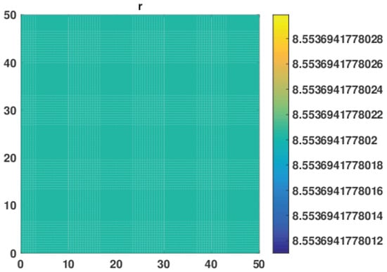
Figure 1. No Patterns for top predator of the model system in Equation (38) were obtained at time level t = 10,000 in the absence of cross diffusion, i.e., self diffusion and cross diffusion coefficients being $d_3=10$, $d_4=0$, respectively.

In our second numerical experiment, we introduced the cross diffusion by gradually increasing the cross diffusivity coefficient $d_4$ and along with that we gradually decreased the self diffusivity coefficient $d_3$. The goal was to see the impact of cross diffusivity on the dynamics when there is very less role of self diffusion in the system. To this end, in Figure 2a, we increase $d_4$ from 0 to $2.3$ and decrease $d_3$ from 10 to $1.7$. An increase in cross diffusion coefficient results in destabilization in the top predator r dynamics leading to a mixture of hot spots and labyrinth patterns, as seen in Figure 2a. We further increased $d_4$ to 5 and decreased $d_3$ to 1 to observe floral turing patterns (Figure 2b).

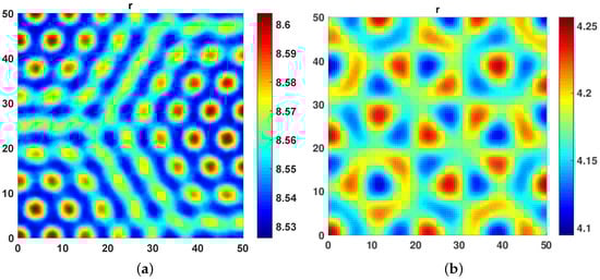
Figure 2. (a) A mix of hot spot and labyrinth turing patterns obtained at $d_3=1.7$ and $d_4=2.3$. (b) Floral Turing patterns obtained at $d_3=1$ and $d_4=5$.

On further increasing the cross diffusivity coefficient at $d_4=6$ and taking self diffusion coefficient at $d_3=0.8$, we observed pentagonal Turing patterns, as shown in Figure 3a. Further, at $d_4=8$ and $d_3=0.3$, we obtained Floral Turing Pattern.

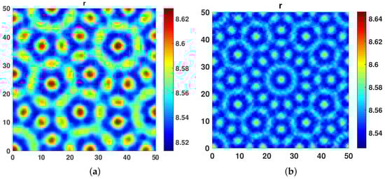
Figure 3. (a) Pentagonal Turing patterns obtained at $d_3=0.8$ and $d_4=6$. (b) Floral Turing patterns obtained at $d_3=0.3$ and $d_4=8$.

Increasing the value of $d_4$ to 10 and fixing $d_3=0.5$, we observed hot spothl turing patterns, as given in Figure 4a at $d_4=15$. At $d_3=0.1$, a mix of hot spot and Labyrinth Turing patterns were observed, as shown in Figure 4b.

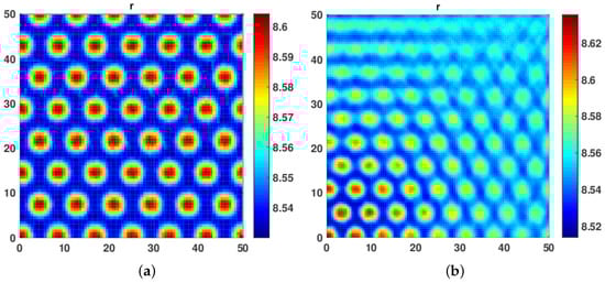
Figure 4. (a) Another hot spot turing patterns obtained at $d_3=0.5$ and $d_4=10$. (b) A mix of Hot Spot and Labyrinth Turing patterns obtained at $d_3=0.1$ and $d_4=15$.

As shown in Figure 5a,b, we observed that, for a very high value of cross diffusion coefficients $d_4=85$ and $d_4=125$, and very low values of $d_3=0.05$ and $d_3=0.06$, hot spot and Hexagonal Spot Turing patterns are obtained, respectively.

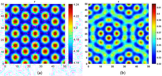
Figure 5. (a) Hot Spot patterns obtained at $d_3=0.05$ and $d_4=85$. (b) Hexagonal Spot Turing patterns obtained at $d_3=0.06$ and $d_4=125$.

From these experiments, we can conclude that the role of cross diffusion in destabilizing the dynamics is much more significant than self diffusion.

In our third numerical experiment, we started with equal values of both $d_3$ and $d_4$ fixed at $0.5$. The hot spot patterns began to appear. Further, when we increased diffusivity coefficient $d_3$ and $d_4$ to 1, a mix of hot spot and Labyrinth Turing Patterns were seen. We further increased both $d_3$ and $d_4$ with the restriction that both self and cross diffusion coefficient must remain the same. We observed that the patterns became more conspicuous, leading to a mix of hot spot and Labyrinth Turing Patterns (see Figure 6a,b and Figure 7a,b).

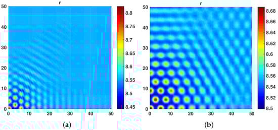
Figure 6. (a) A mixture of Hot Spot and Labyrinth Turing patterns obtained at $d_3=d_4=0.5$. (b) A mix of Hot Spot and Labyrinth Turing patterns obtained at $d_3=d_4=1$.

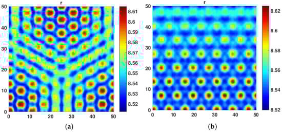
Figure 7. (a) A mixture of hot spot and labyrinth turing patterns obtained at $d_3=d_4=1.5$. (b) A mixture of hot spot and labyrinth turing patterns obtained at $d_3=d_4=2$.

Through extensive simulations over a wide range of diffusivity coefficients, we observed that cross diffusion coefficient $d_4$ plays an important role to realize the phenomenon of pattern formation. In the absence of cross diffusion, no patterns were formed, even at higher values of $d_3$, as shown in Figure 1. Moreover we also determined the Turing patterns in the cases where cross diffusion coefficient equals to the self diffusion coefficient, i.e., $d_3=d_4$. Table 1 describes the various self and cross diffusivity coefficients used for obtaining the spatial patterns of the system in Equation (38). Table 1 indicates a negative correlation between self diffusion coefficient and cross diffusion coefficients, which results in pattern formation. The above simulations results are coherent to our analytical results that non-constant positive solutions exist only in the presence of cross diffusion hence the pattern formation.

7. Conclusions

In this study, we concluded a three-dimensional continuous time ecological system, modeling a tritrophic food chain based on a hybrid type of Holling Type II and Crowley-Martin functional response. We also took into account inhomogeneous spatial distribution of the species involved and dependence of movements of the species on the population density due to the mutual interference between the individuals of the same species and included nonlinear self diffusion and cross diffusion in our discussion. We established that, under certain parametric conditions, the model is unstable only in the presence of cross diffusion. This phenomenon can be regarded as an extension to diffusion driven instability and can be referred to as cross diffusion driven instability. The phenomenon of pattern formation in spatially extended models including cross diffusion as a destabilizing mechanism was studied with varying the self diffusion and cross diffusion coefficients over a wide range, which serves as an extension to Turing pattern formations exhibited by reaction diffusion system. In addition, we analytically proved the existence of inhomogeneous steady states and gave a priori upper and lower bounds for the positive solutions of the system under steady state. We proved that no non-constant positive solutions exist in the presence of only self diffusion subject to certain conditions. Through simulation, we concluded that cross diffusion is necessary for pattern formation of models in which species interactions are governed by Crowley-Martin and Holling Type II functional response. This establishes the fact that Crowley-Martin functional response governed species interaction is stable in spatial temporal aspects when the species diffuse because of their own characteristic behavior but when under the influence of other species the system tends towards instability. Based on our analysis and simulation, we concluded that cross diffusion induces at least a inhomogeneous stationary solution and mathematically explains the segregation phenomenon of ecosystem under the influence of predator dependent functional response.

References

- Kuang, Y.; Beretta, E. Global qualitative analysis of a ratio-dependent predator-prey system. J. Math. Biol. 1998, 36, 389–406. [Google Scholar] [CrossRef]
- Segel, L.A. Modeling Dynamic Phenomena in Molecular and Cellular Biology; Cambridge University Press: Cambridge, UK, 1984. [Google Scholar]
- Price, P.W.; Bouton, C.E.; Gross, P.; McPheron, B.A.; Thompson, J.N.; Weis, A.E. Interactions among three trophic levels: influence of plants on interactions between insect herbivores and natural enemies. Annu. Rev. Ecol. Syst. 1980, 11, 41–65. [Google Scholar] [CrossRef]
- Hastings, A.; Powell, T. Chaos in a three-species food chain. Ecology 1991, 72, 896–903. [Google Scholar] [CrossRef]
- McCann, K.; Yodzis, P. Biological Conditions for Chaos in a Three-Species Food Chain. Ecology 1994, 75, 561–564. [Google Scholar] [CrossRef]
- Gakkhar, S.; Naji, R.K. Chaos in three species ratio dependent food chain. Chaos Solitons Fractals 2002, 14, 771–778. [Google Scholar] [CrossRef]
- Rai, V.; Upadhyay, R.K. Chaotic population dynamics and biology of the top-predator. Chaos Solitons Fractals 2004, 21, 1195–1204. [Google Scholar] [CrossRef]
- Crowley, P.H.; Martin, E.K. Functional responses and interference within and between year classes of a dragonfly population. J. N. Am. Benthol. Soc. 1989, 8, 211–221. [Google Scholar] [CrossRef]
- Upadhyay, R.K.; Naji, R.K. Dynamics of a three species food chain model with Crowley Martin type functional response. Chaos Solitons Fractals 2009, 42, 1337–1346. [Google Scholar] [CrossRef]
- Turing, A.M. The chemical basis of morphogenesis. Philos. Trans. R. Soc. Lond. B 1952, 237, 37–72. [Google Scholar]
- Kondo, S. The reaction-diffusion system: a mechanism for autonomous pattern formation in the animal skin. Genes Cells 2002, 7, 535–541. [Google Scholar] [CrossRef] [PubMed]
- Kondo, S.; Miura, T. Reaction-diffusion model as a framework for understanding biological pattern formation. Science 2010, 329, 1616–1620. [Google Scholar] [CrossRef] [PubMed]
- Dong, Y.; Zhang, S.; Li, S.; Li, Y. Qualitative Analysis of a Predator-Prey Model with Crowley-Martin Functional Response. Int. J. Bifurc. Chaos 2015, 25, 1550110. [Google Scholar] [CrossRef]
- Kuto, K. Stability of steady-state solutions to a prey-predator system with cross-diffusion. J. Differ. Equ. 2004, 197, 293–314. [Google Scholar] [CrossRef]
- Kuto, K.; Yamada, Y. Multiple coexistence states for a prey-predator system with cross-diffusion. J. Differ. Equ. 2004, 197, 315–348. [Google Scholar] [CrossRef]
- Pang, P.Y.H.; Wang, M. Strategy and stationary pattern in a three-species predator-prey model. J. Differ. Equ. 2004, 200, 245–273. [Google Scholar] [CrossRef]
- Wang, M. Stationary patterns caused by cross-diffusion for a three-species prey-predator model. Comput. Math. Appl. 2006, 52, 707–720. [Google Scholar] [CrossRef]
- Tian, C. Turing patterns created by cross-diffusion for a Holling II and Leslie-Gower type three species food chain model. J. Math. Chem. 2011, 49, 1128–1150. [Google Scholar] [CrossRef]
- Tian, C.; Ling, Z.; Lin, Z. Spatial patterns created by cross-diffusion for a three-species food chain model. Int. J. Biomath. 2014, 7, 1450013. [Google Scholar] [CrossRef]
- Medvinsky, A.B.; Petrovskii, S.V.; Tikhonova, I.A.; Malchow, H.; Li, B.-L. Spatiotemporal complexity of plankton and fish dynamics. SIAM Rev. 2002, 44, 311–370. [Google Scholar] [CrossRef]
© 2019 by the authors. Licensee MDPI, Basel, Switzerland. This article is an open access article distributed under the terms and conditions of the Creative Commons Attribution (CC BY) license (http://creativecommons.org/licenses/by/4.0/).