Switching Point Solution of Second-Order Fuzzy Differential Equations Using Differential Transformation Method

Abstract

The first-order fuzzy differential equation has two possible solutions depending on the definition of differentiability. The definition of differentiability changes as the product of the function and its first derivative changes its sign. This switching of the derivative’s definition is handled with the application of min, max operators. In this paper, a numerical technique for solving fuzzy initial value problems is extended to solving higher-order fuzzy differential equations. Fuzzy Taylor series is used to develop the fuzzy differential transformation method for solving this problem. This leads to a single solution for higher-order differential equations.

1. Introduction

The fuzzy set theory was pioneered by Lotfi Zadeh [1]. Fuzzy sets are widely used in a variety of mathematical modeling, and fuzzy derivative was introduced in [2,3,4,5,6,7,8,9] and is an extension of ordinary derivatives. This provides the foundation of fuzzy differential equations, and uncertain systems are modeled using fuzzy differential equations.

Fuzzy differential equations are solved using many methods, such as differential or fuzzy inclusion [10,11,12], the extension principle and characterization theorem [13,14,15], and artificial neural networks [16]. Numerical methods such as the differential transformation method [17,18], extension of numerical solution methods for ordinary differential equations (ODEs) [19,20,21,22,23,24], interactive derivatives [25], multistep methods [26], and Runge–Kutta (RK) methods [27] are also applied to solving these equations. The metric properties of fuzzy functions are studied in [28,29]. The existence of solutions for second-order fuzzy differential equations is proved in [21,30]. As a result, higher-order fuzzy differential equations can be solved by using generalized fuzzy derivatives. A system of differential equations and second-order differential equations are solved in [6,31].

A first-order differential equation with an initial value is called an initial value problem, and this sort of equation has a unique solution. If the initial values are fuzzified, then the problem is called a fuzzy initial value problem (FIVP). The differential equation with fuzzy initial values has two solutions for every fuzzification parameter. These solutions depend upon the definition of fuzzy differentiability, and the definition changes as the sign of the product of function and its first derivative change [32].

Fuzzy differential equations are interpreted as a family of differential inclusions. Fuzzy interval arithmetic is very simple to compute because it is applicable to the endpoints of an interval, and this leads to an estimate of the confidence interval. These fuzzy solutions are constructed from the solution of the crisp problem generated by the fuzzy initial value problem. Fuzzy solutions are developed using the parametric representation of fuzzy functions. In this representation, fuzzy sets are represented by lower and upper approximations: the lower approximation is increasing and the upper approximation is a decreasing function. The function’s property of increasing and decreasing is utilized with the definition of switching points. The fuzzy differentiability of type-(i) switches to that of type-(ii) at the point where the function changes its increasing nature to decreasing or vice versa. This property is also used for the first-order derivative function, and similar logic is implemented for developing the solution of second-order differential equations.

The differential transformation method (DTM) [33] is a way of finding the numerical solution of linear and nonlinear differential equations [34]. The DTM is also used for solving fuzzy differential equations (FDEs) with FIVPs [10,35]. In this paper, a solution of a second-order fuzzy differential equation is proposed. The second-order differential equation is converted to an equal system of first-order differential equations, and initial values are fuzzified. The switching points are verified for the solution and first-order derivative functions. The DTM is used to solve the system of equations, and the solution leads to the approximation of a fuzzy solution of the problem.

Two-point initial value problems are considered in [14,36,37,38], and a fuzzy boundary value problem is solved in [39]. In these approaches, the definition of differentiability in the given interval is chosen initially without switching. In this paper, the FIVP is approached by using FDTM, and the idea is extended to second-order fuzzy differential equations with the adaptability of min and max operators to handle the switching points. The solution set produces the upper and lower approximations for the bounded solution of the second-order differential equation. The first-order FIVP represents a single solution with the application of two definitions of differentiability, and for second-order FIVP, the four definitions of differentiability are combined with the application of min, max operators, where the definition of differentiability depends upon the interval of the validity of the solution and the switching point within that interval. This leads to a unique solution of the differential equation. The rest of the paper is organized as follows: First, we start with preliminaries in Section 2. The switching points and fuzzy differentiability for second-order derivatives are explained in Section 3. In Section 4, we describe the DTM, and its extension is derived in Section 4.1. In Section 5, numerical examples are discussed, and finally, Section 7 consists of the conclusion with a summary of our contribution, as well as a discussion of future directions of investigation.

2. Preliminaries

Numerous techniques and terms are used to define a fuzzy number and fuzzy membership functions [40]. In this paper, the following definitions are used.

Definition 1

(Fuzzy Set). An ordered pair of a set and a membership function is called a fuzzy set, and a membership function is defined as $\eta :R\to [0,1]$. The fuzzy set has the following properties:

1. 

A set of all the points where the membership function has a nonzero value is called the support of the fuzzy set.

2. 

The set of points where $\eta \left(x\right)=1$ is called the core of a fuzzy set η.

3. 

A fuzzy set η is normal if ∃ at least one $x_0\in R$ such that $\eta \left(x_0\right)=1$.

4. 

A fuzzy set η is convex if $\eta (tx+(1-t\left)y\right)\ge min\left(\eta \right(x),\eta (y\left)\right)$ for all $x,y\in R$ and $t\in [0,1]$.

5. 

A fuzzy set is upper semi-continuous in R

6. 

Compactness of a fuzzy set is defined as $\overline{|x\in R,\eta \left(x\right)>0|}$, where $\overline{.}$ stands for a closure operator.

The fuzzy real numbers, numbers with a triangular sendograph, are represented by $E^1$ such that $R\subset E$. These fuzzy number are represented as three points, $a,b,c\in R$, with $a<b<c$; then, the $\alpha$-level fuzzy set is represented by $\underline{h}\left(\gamma \right)=a+(b-a)\gamma$ and $\overline{h}\left(\gamma \right)=c-(c-b)\gamma$. The $\gamma$ cuts for all $0<\gamma \le 1$ are defined as ${\left[h\right]}_{\gamma }=\{h\left(x\right)\ge \gamma \forall x\in R\}$. These are called the level sets, and the zero-level compact set is represented by ${\left[h\right]}_0=\overline{\left\{h\right(x)>0\mathrm{for}\mathrm{all}x\in R\}}$. The level sets are nested sets, and the $\gamma$ cuts of any fuzzy number are always closed and bounded intervals.

Definition 2.

Fuzzy numbers are represented as an ordered pair of functions $(\underline{h}\left(\gamma \right),\overline{h}\left(\gamma \right))$, where $\gamma \in [0,1]$, and $\underline{h}\left(\gamma \right)$ and $\overline{h}\left(\gamma \right)$ are called the lower and upper boundaries of $h\left(\gamma \right)$. The $\overline{h}\left(\gamma \right)$ is bounded, left continuous, and decreasing, and $\underline{h}\left(\gamma \right)$ is bounded, right continuous, and an increasing function on $[0,1]$, and $\underline{h}\left(\gamma \right)\le \overline{h}\left(\gamma \right)$ for all $\gamma \in [0,1]$. A crisp number is represented by an equivalent fuzzy notation with an equal approximation of lower and upper $h\left(\gamma \right)$. Let h and g be two fuzzy numbers defined in γ-level notation, where $h=(\underline{h},\overline{h})$ and $g=(\underline{g},\overline{g})$; then, the algebra of fuzzy numbers is defined as

Addition: 

Two fuzzy numbers h and g are added as follows: $\underline{(h+g)}\left(\gamma \right)=\underline{h}\left(\gamma \right)+\underline{g}\left(\gamma \right)$ and $\overline{(h+g)}\left(\gamma \right)=\overline{h}\left(\gamma \right)+\overline{g}\left(\gamma \right)$, and its γ-level addition will be ${[h+g]}_{\gamma }=[\underline{(h+g)}\left(\gamma \right),\overline{(h+g)}\left(\gamma \right)]$

Subtraction: 

The subtraction of fuzzy triangular numbers is computed as follows: $\underline{(h-g)}\left(\gamma \right)=\underline{h}\left(\gamma \right)-\underline{g}\left(\gamma \right)$ and $\overline{(h-g)}\left(\gamma \right)=\overline{h}\left(\gamma \right)-\overline{g}\left(\gamma \right)$. The subtraction of fuzzy numbers $h-g$ is defined as addition, and the parameterized subtraction is defined as ${[h-g]}_{\gamma }=[\underline{(h-g)}\left(\gamma \right),\overline{(h-g)}\left(\gamma \right)]$

Scalar Multiplication: 

The scalar multiplication of a scalar a with a fuzzy number is computed as follows: $\underline{ah}\left(\gamma \right)=a\underline{h}\left(\gamma \right),\overline{ah}\left(\gamma \right)=a\overline{h}\left(\gamma \right)$ when $a\ge 0$ and $\underline{ah}\left(\gamma \right)=a\overline{h}\left(\gamma \right),\overline{ah}\left(\gamma \right)=a\underline{h}\left(\gamma \right)$ when $a<0$, and the scalar multiplication will become $a{h}_{\gamma }=[\underline{ah}\left(\gamma \right),\overline{ah}\left(\gamma \right)]$

Multiplication: 

Let $h,g$ be two fuzzy numbers; then, multiplication of fuzzy numbers is computed as follows: $hg=[\underline{hg},\overline{hg}]$, where $\underline{\left(hg\right)}\left(\gamma \right)=min[\underline{h}\left(\gamma \right)\underline{g}\left(\gamma \right),\overline{h}\left(\gamma \right)\underline{g}\left(\gamma \right),\underline{h}\left(\gamma \right)\overline{g}\left(\gamma \right),\overline{h}\left(\gamma \right)\overline{g}\left(\gamma \right)]$ and $\overline{\left(hg\right)}\left(\gamma \right)=max[\underline{h}\left(\gamma \right)\underline{g}\left(\gamma \right),\overline{h}\left(\gamma \right)\underline{g}\left(\gamma \right),\underline{h}\left(\gamma \right)\overline{g}\left(\gamma \right),\overline{h}\left(\gamma \right)\overline{g}\left(\gamma \right)]$

Division: 

Division between two fuzzy numbers is defined conditionally. If $0\notin [{\underline{g}}_0,{\overline{g}}_0]$, then $\frac{u}{v}=[\underline{\left(\frac{h}{g}\right)},\overline{\left(\frac{h}{g}\right)}]$ is defined as $\underline{\left(\frac{h}{g}\right)}\left(\gamma \right)=min[\frac{\underline{h}\left(\gamma \right)}{\underline{g}\left(\gamma \right)},\frac{\overline{h}\left(\gamma \right)}{\underline{g}\left(\gamma \right)},\frac{\underline{h}\left(\gamma \right)}{\overline{g}\left(\gamma \right)},\frac{\overline{h}\left(\gamma \right)}{\overline{g}\left(\gamma \right)}]$ and $\overline{\left(\frac{h}{g}\right)}\left(\gamma \right)=max[\frac{\underline{h}\left(\gamma \right)}{\underline{g}\left(\gamma \right)},\frac{\overline{h}\left(\gamma \right)}{\underline{g}\left(\gamma \right)},\frac{\underline{h}\left(\gamma \right)}{\overline{g}\left(\gamma \right)},\frac{\overline{h}\left(\gamma \right)}{\overline{g}\left(\gamma \right)}]$

Definition 3

(H-Difference). The set of real numbers is defined by fuzzy membership function E, and $h,g,f$ are three fuzzy numbers in E such that $h=g+f\iff h-g=f$. Then, the H-difference of two fuzzy real numbers is denoted as $h\ominus g$. Its γ-level representation will become

$${[h\ominus g]}_{\gamma }=[{\underline{h}}_{\gamma }-{\overline{g}}_{\gamma },{\overline{h}}_{\gamma }-{\underline{g}}_{\gamma }].$$

Definition 4

(g-Difference). The set of real numbers is defined by fuzzy membership function E, and $h,g,f$ are three fuzzy numbers in E such that $h=g+f\iff h-g=f$. Then, the g-difference of two fuzzy real numbers is defined as $x{\ominus }_{g}y$, and its γ cuts are

$${\left[u{\ominus }_{g}v\right]}_{\gamma }={\cup }_{\beta \ge \gamma }[{\underline{h}}_{\beta }{\ominus }_{gh}{\underline{g}}_{\beta },{\overline{h}}_{\beta }{\ominus }_{gh}{\overline{g}}_{\beta }].$$

Definition 5

(Hausdorff Distance). Let $F:R_f\times R_f\to R_{+}\cup \left\{0\right\}$ be a function. Then, the Hausdorff distance is defined as

$$D(u,v)=Su{p}_{\gamma \in [0,1]}max\{\mid {\underline{h}}_{\gamma }-{\underline{v}}_{\gamma }\mid ,\mid {\overline{h}}_{\gamma }-{\overline{v}}_{\gamma }\mid \}=\mid \mid {\left[u\right]}_{\gamma }{\ominus }_g{\left[v\right]}_{\gamma }\mid \mid ,$$

where a complete metric space is represented by D. The g-difference of intervals always exists. This definition is equivalent to the usual definitions for metric spaces of fuzzy numbers.

Definition 6

(Generalized Hukuhara Difference). The generalized Hukuhara difference between two fuzzy numbers is defined as a and b as follows:

$${\left[a{\ominus }_{gH}b\right]}_{\gamma }=[{\underline{c}}_{\gamma },{\overline{c}}_{\gamma }]$$

where ${\underline{c}}_{\gamma }=min({\underline{a}}_{\gamma }-{\underline{a}}_{\gamma },{\overline{a}}_{\gamma }-{\overline{a}}_{\gamma })$ and ${\overline{c}}_{\gamma }=max({\underline{a}}_{\gamma }-{\underline{a}}_{\gamma },{\overline{a}}_{\gamma }-{\overline{a}}_{\gamma })$ with the conditions that ${\underline{c}}_{\gamma }$ is a nondecreasing function and ${\overline{c}}_{\gamma }$ is a nonincreasing function such that ${\underline{c}}_{\gamma }<{\overline{c}}_{\gamma }$.

Definition 7

(Generalized Hukuhara Differentiability [41]). Let f be a fuzzy function and $f:[a,b]\to K_F\left(R^n\right)$, and let t be any point in the domain. Then, f is a strongly generalized differentiable function f at t and will be defined by the following.

for all$h>0$If h is sufficiently small and $h>0$, then

• Differentiable type-(i): There exist $f(t+h)\ominus f\left(t\right)$ and $f\left(t\right)\ominus f(t-h)$; then,

  $$f^{\prime }\left(t\right)=\underset{h\to 0}{lim}\frac{f(t+h)\ominus f\left(t\right)}{h}=\underset{h\to 0}{lim}\frac{f\left(t\right)\ominus f(t-h)}{h}$$

  (1)

  or
• Differentiable type-(ii): If $f\left(t\right)\ominus f(t+h)$ and $f(t-h)\ominus f\left(t\right)$ exist and

  $$f^{\prime }\left(t\right)=\underset{h\to 0}{lim}\frac{f(t+h)\ominus f\left(t\right)}{-h}=\underset{h\to 0}{lim}\frac{f\left(t\right)\ominus f(t-h)}{-h}$$

  (2)

for all$h<0$If h is sufficiently small and $h<0$, then

• Differentiable type-(i): There exist $f(t+h)\ominus f\left(t\right)$ and $f\left(t\right)\ominus f(t-h)$; then,

  $$f^{\prime }\left(t\right)=\underset{h\to 0}{lim}\frac{f(t-h)\ominus f\left(t\right)}{-h}=\underset{h\to 0}{lim}\frac{f\left(t\right)\ominus f(t+h)}{-h}$$

  (3)
• Differentiable type-(ii): There exist $f\left(t\right)\ominus f(t+h)$ and $f(t-h)\ominus f\left(t\right)$; then,

  $$f^{\prime }\left(t\right)=\underset{h\to 0}{lim}\frac{f(t-h)\ominus f\left(t\right)}{h}=\underset{h\to 0}{lim}\frac{f\left(t\right)\ominus f(t+h)}{h}$$

  (4)

Reasoning as above, there exists the Hukuhara difference $f\left(x_0\right){\ominus }_{H}f(x_0-h)$. Now, if we suppose $f^{\prime }<0$, then we see that we cannot use the above kind of reasoning to prove that the H-differences $f(x_0+h){\ominus }_{H}f\left(x_0\right)$ and $f\left(x_0\right){\ominus }_{H}f(x_0-h)$ and the derivative $f^{\prime }\left(x_0\right)$ exist.

Definition 8

(Second-Order Generalized Hukuhara Differentiability [41]). Let $f^{\prime }$ be a strongly differentiable function in the generalized sense on the domain, and let there exist $f^{″}\left(t\right)\in R_f$ such that, for all $h>0$, we have

(I) 

$\exists f^{\prime }(t+h)\ominus f^{\prime }\left(t\right)$ and $\exists f^{\prime }\left(t\right)\ominus f^{\prime }(t-h)$ and

$$f^{″}\left(t\right)=\underset{h\to 0}{lim}\frac{f^{\prime }(t+h)\ominus f^{\prime }\left(t\right)}{h}=\underset{h\to 0}{lim}\frac{f^{\prime }\left(t\right)\ominus f^{\prime }(t-h)}{h}$$

(II) 

$\exists f^{\prime }\left(t\right)\ominus f^{\prime }(t+h)$ and $\exists f^{\prime }(t-h)\ominus f^{\prime }\left(t\right)$ and

$$f^{″}\left(t\right)=\underset{h\to 0}{lim}\frac{f^{\prime }(t-h)\ominus f^{\prime }\left(t\right)}{-h}=\underset{h\to 0}{lim}\frac{f^{\prime }\left(t\right)\ominus f^{\prime }(t+h)}{-h}$$

If f has differentiability of type-(i) and $f^{″}$ exists, then there are two possibilities for the differentiability of function $f^{\prime }$. Similarly, if f has differentiability of type-(ii), then $f^{\prime }$ has two possibilities. Thus $f^{″}$ has four definitions of differentiability.

Definition 9

(Generalized Differentiability ([42])). Let $x_0\in [a,b]$ and k be such that $x_0+k\in [a,b]$; then, the g_derivative of the function $f:[a,b]\to K_F\left(R^n\right)$ at $x_0$ is defined as

$$f_g^{\prime }\left(x_0\right)=\underset{k\to 0}{lim}\frac{1}{k}\left[f(x_0+k){\ominus }_{g}f\left(x_0\right)\right].$$

(5)

If $f_g^{\prime }\left(x_0\right)$ exists, then f is called differentiable in the generalized sense.

Theorem 1.

Let $F:[a,b]\to K_F\left(R^n\right)$ be such that

$${\left[F\left(x\right)\right]}_{\gamma }=[f{\left(x\right)}_{\gamma },g{\left(x\right)}_{\gamma }]$$

where $(f{\left(x\right)}_{\gamma }$ and $g{\left(x\right)}_{\gamma }$ are differentiable real-valued functions with respect to x. Then, $F\left(x\right)$ is g_ differentiable, and mathematically,

$${\left[F^{\prime }\left(x\right)\right]}_{\gamma }=[min({\left(f^{\prime }\left(x\right)\right)}_{\gamma },{\left(g^{\prime }\left(x\right)\right)}_{\gamma }),max({\left(f^{\prime }\left(x\right)\right)}_{\gamma },{\left(g^{\prime }\left(x\right)\right)}_{\gamma })]$$

The interval is divided into subintervals. The functional value at the end point of the previous interval becomes the initial value of the next subinterval and at each boundary point of the subinterval. The conditions are verified, and if there is a switching point, then the definition of fuzzy derivative changes from type-(i) to type-(ii) and vice versa. The use of min and max operators handles the switching points, which are defined in the next subsection. (Proof of Theorem 1 follows from [42].)

Proposition 1.

([43]) Let $F:(t_0+a,T)\to K_F\left(R^n\right)$ be Hukuhara differentiable 2 times and

$$[{\left(F^{\prime }\right)}_{\gamma }\left(t\right))]=[{\left(f_1^{\prime }\right)}_{\gamma }\left(t\right)),{\left(f_2^{\prime }\right)}_{\gamma }\left(t\right)\left)\right]\gamma \in [0,1]$$

such that ${\left(f_1^{\prime }\right)}_{\gamma }\left(t\right))=min({\left(f^{\prime }\left(x\right)\right)}_{\gamma },{\left(g^{\prime }\left(x\right)\right)}_{\gamma })$ and ${\left(f_2^{\prime }\right)}_{\gamma }\left(t\right))=max({\left(f^{\prime }\left(x\right)\right)}_{\gamma },{\left(g^{\prime }\left(x\right)\right)}_{\gamma })$. If $f^{\prime },g^{\prime }$ are differentiable, then we can write $F^{\left(2\right)}$ in a similar fashion:

$$[F_{\gamma }^{\left(2\right)}\left(t\right))]=[{(f_1^{\left(2\right)})}_{\gamma }\left(t\right)),{\left(f_2^{\left(2\right)}\right)}_{\gamma }\left(t\right)\left)\right]\gamma \in [0,1]$$

In fact, the second-order derivative of a real-valued function represents the four definitions of fuzzy derivatives of fuzzy functions. The definition of the derivative changes at the switching point.

Theorem 2

(Theorem 3.6 in [41]). Let $F:R\to E$ be a function and denote $F{\left(t\right)}_{\gamma }=[f{\left(t\right)}_{\gamma },g{\left(t\right)}_{\gamma }]$ for each $\gamma \in [0,1]$. Then,

• If F is (I)-differentiable, then f and g are differentiable functions and $D_1^{1}F{\left(t\right)}_{\gamma }=F^{\prime }{\left(t\right)}_{\gamma }=[f^{\prime }{\left(t\right)}_{\gamma },g^{\prime }{\left(t\right)}_{\gamma }]$
• If f is (II)-differentiable, then f and g are differentiable functions and $D_2^{1}F{\left(t\right)}_{\gamma }=F^{\prime }{\left(t\right)}_{\gamma }=[g^{\prime }{\left(t\right)}_{\gamma },f^{\prime }{\left(t\right)}_{\gamma }]$.

Proof. 

For details, see [41]. □

Theorem 3

(Theorem 3.9 in [41]). Let $\left[f\right(t\left)\right]=\left[f\right(t),g(t\left)\right]$ be an interval-valued function, where f is an increasing function and g is a decreasing function, and let the system $D_1^{\left(1\right)}f:I\mapsto R_f$ and $D_2^{\left(1\right)}f:I\mapsto R_f$ be two fuzzy functions. Then,

1. 

Let $f^{\prime }$ and $g^{\prime }$ be two differentiable functions. If F and $D_1^{\left(1\right)}F$ are (I)-differentiable, then $D_{1,1}^{\left(2\right)}{\left[F\left(t\right)\right]}_{\gamma }=[f^{″}{\left(t\right)}_{\gamma },g^{″}{\left(t\right)}_{\gamma }]$.

2. 

Let $f^{\prime }$ and $g^{\prime }$ be two differentiable functions. If F is (I)-differentiable and $D_1^{\left(1\right)}F$ is (II)-differentiable, then $D_{1,2}^{\left(2\right)}{\left[F\left(t\right)\right]}_{\gamma }=[g^{″}{\left(t\right)}_{\gamma },f^{″}{\left(t\right)}_{\gamma }]$.

3. 

Let $f^{\prime }$ and $g^{\prime }$ be two differentiable functions. If F is (II)-differentiable and $D_1^{\left(1\right)}F$ is (I)-differentiable, then $D_{2,1}^{\left(2\right)}{\left[F\left(t\right)\right]}_{\gamma }=[g^{″}{\left(t\right)}_{\gamma },f^{″}{\left(t\right)}_{\gamma }]$.

4. 

Let $f^{\prime }$ and $g^{\prime }$ be two differentiable functions. If F and $D_1^{\left(1\right)}F$ are (II)-differentiable, then $D_{2,2}^{\left(2\right)}{\left[F\left(t\right)\right]}_{\gamma }=[f^{″}{\left(t\right)}_{\gamma },g^{″}{\left(t\right)}_{\gamma }]$.

Proof. 

For details, see [41]. □

Theorem 4

(Theorem 3.1 in [44]). Let $t_0\in [a,b]$ and assume that $f:[a,b]\times R_F\to R_F$ is continuous. A mapping $x:[a,b]\to R_F$ is a solution to the initial value problem $x^{″}=f(t;x;x^{\prime })$ and $x\left(t_0\right)=k_1;x^{\prime }\left(t_0\right)=k_2$ if and only if x and $x^{\prime }$ are continuous and satisfy one of the following conditions:

• $x\left(t\right)=k_2(t-t_0)+\underset{t_0}{\overset{t}{\int }}(\underset{t_0}{\overset{t}{\int }}f(s,x\left(s\right),x^{\prime }\left(s\right))ds)ds+k_1$, where $x^{\prime }$ and $x^{″}$ are (i)-differentials,
• $x\left(t\right)=k_1\ominus (-1)(k_2(t-t_0)\ominus (-1)\underset{t_0}{\overset{t}{\int }}(\underset{t_0}{\overset{t}{\int }}f(s,x\left(s\right),x^{\prime }\left(s\right))ds)ds$, where $x^{\prime }$ and $x^{″}$ are (ii)-differentials,
• $x\left(t\right)=k_1\ominus (-1)(k_2(t-t_0)+\underset{t_0}{\overset{t}{\int }}(\underset{t_0}{\overset{t}{\int }}f(s,x\left(s\right),x^{\prime }\left(s\right))ds)ds$, where $x^{\prime }$ is (i)-differentiable and $x^{″}$ is a (ii)-differential, or
• $x\left(t\right)=k_2(t-t_0)k_1\ominus (-1)\underset{t_0}{\overset{t}{\int }}(\underset{t_0}{\overset{t}{\int }}f(s,x\left(s\right),x^{\prime }\left(s\right))ds)ds+k_1$, where $x^{\prime }$ is (ii)-differentiable and $x^{″}$ is a (i)-differential.

Remark 1.

(i) This theorem shows that four systems of fuzzy differentiability represent only two systems, and two pairs are equivalent. According to the conditions of the triangular fuzzy function, f is an increasing function and g is a decreasing function. If F follows the first definition, then $F^{\prime }=[f^{\prime },g^{\prime }]$. This shows that $f^{\prime }$ is an increasing function and $g^{\prime }$ is a decreasing function. In the other case, $F^{\prime }=[g^{\prime },f^{\prime }]$, which shows that $f^{\prime }$ is now decreasing and $g^{\prime }$ is an increasing function. (ii) Theorem 4 is for H-differentiability, and its mode-generalized form is $gH$ differentiability, so it is also $gH$ differentiable.

3. Fuzzy Differentiability and Switching Points

Definition 10

(Switching Point). The points in an interval where fuzzy differentiability of type-(i) changes to type-(ii) and vice versa are called switching points.

For the first-order initial value differential equations, the above-cited switching points apply. This logic can be derived from any one of the two functions f and g, and the definition of fuzzy differentiability is associated with any of the above functions. In

Table 1. Nature of the function and type of differentiability; ↗ and ↘ stand for increasing and decreasing functions, respectively.

S. N.	f	${\mathit{f}}^{\prime }$	Relationship with Derivatives of g	Differentiability
1	↗	↗	$f^{\prime }<g^{\prime }$	type-(i)
2	↗	↘	$f^{\prime }>g^{\prime }$	type-(ii)

, f is increasing. The definition changes from type-(i) to type-(ii) if f changes its increasing nature to decreasing and vice versa.

The possibility for f is described in the Table 1. If both the function and its derivative are increasing functions (similarly for g decreasing) then, type-(i) is applicable, if $f^{\prime }$ changes its nature and is a decreasing function then differentiability of type-(ii) is applicable. This behavior of function is verified over the interval. We extend the same logic to the second derivative, and we get the representations listed in

Table 2. Nature of second-order derivatives and their relationship with derivatives of g.

S. N.	f	${\mathit{f}}^{\prime }$	${\mathit{f}}^{\left(2\right)}$	Relationship with Derivatives of g	Type of Differentiability
1	↗	↗	↗	$f^{\prime }<g^{\prime }$ and $f^{\left(2\right)}<g^{\left(2\right)}$	f and $f^{\prime }$ have differentiability type-(I), and the system $D_{1,1}^{\left(2\right)}$ is also type-(I)
2	↗	↗	↘	$f^{\prime }<g^{\prime }$ and $f^{\left(2\right)}>g^{\left(2\right)}$	f follows type-(I), $f^{\prime }$ has type-(II), and $D_{1,2}^{\left(2\right)}$ is also type-(II)
3	↗	↘	↘	$f^{\prime }>g^{\prime }$ and $f^{\left(2\right)}>g^{\left(2\right)}$	f follows type-(II), $f^{\prime }$ has type-(I), and the system is represented by $D_{2,1}^{\left(2\right)}$
4	↗	↘	↗	$f^{\prime }>g^{\prime }$ and $f^{\left(2\right)}>g^{\left(2\right)}$	f and $f^{\prime }$ have differentiability type-(II), and the system $D_{2,2}^{\left(2\right)}$ is also type-(II)

.

The above table shows that the fuzzy function follows the same differentiability if there is no switch in increasing or decreasing nature of function or there are two switches. The pair with one switching point also have similar behavior. We transform the second-order differential equation into equal system of first-order differential equations.

$$y^{″}\left(t\right)=f(t,y\left(t\right),y^{\prime }\left(t\right))$$

(6)

This second-order differential equation is decomposed into the system of first-order differential equation as

$$\begin{array}{cc}\hfill y{1}^{\prime }\left(t\right)& =y2\left(t\right)\hfill \\ \hfill y{2}^{\prime }\left(t\right)& =f(t,y1(t),y2(t\left)\right)\hfill \end{array}$$

where transformation $y1\left(t\right)=y\left(t\right)$ and $y2\left(t\right)=y^{\prime }\left(t\right)$ is used to describe the equivalent system of first-order differential equations.

The solution system described in [36] will become

• I-I system:

  $$\begin{array}{cccc}\hfill {\underline{y1}}^{\prime }(t,\gamma )& =\underline{y2}(t,\gamma ),\hfill & \hfill {\underline{y2}}^{\prime }(t,\gamma )& =\underline{f}(t,\underline{y1}(t,\gamma ),\overline{y1}(t,\gamma ),\underline{y2}(t,\gamma ),\overline{y2}(t,\gamma ))\hfill \\ \hfill {\overline{y1}}^{\prime }(t,\gamma )& =\overline{y2}(t,\gamma ),\hfill & \hfill {\overline{y2}}^{\prime }(t,\gamma )& =\overline{f}(t,\underline{y1}(t,\gamma ),\overline{y1}(t,\gamma ),\underline{y2}(t,\gamma ),\overline{y2}(t,\gamma ))\hfill \\ \hfill \underline{y1}(0,\gamma )& ={\underline{y1}}_0\left(\gamma \right),\hfill & \hfill \overline{y1}(0,\gamma )={\overline{y1}}_0\left(\gamma \right)\\ \hfill \underline{y2}(0,\gamma )& ={\underline{y2}}_0\left(\gamma \right),\hfill & \hfill \overline{y2}(0,\gamma )={\overline{y2}}_0\left(\gamma \right)\end{array}$$
• I-II system:

  $$\begin{array}{cccc}\hfill {\underline{y1}}^{\prime }(t,\gamma )& =\underline{y2}(t,\gamma ),\hfill & \hfill {\underline{y2}}^{\prime }(t,\gamma )& =\overline{f}(t,\underline{y1}(t,\gamma ),\overline{y1}(t,\gamma ),\underline{y2}(t,\gamma ),\overline{y2}(t,\gamma ))\hfill \\ \hfill {\overline{y1}}^{\prime }(t,\gamma )& =\overline{y2}(t,\gamma ),\hfill & \hfill {\overline{y2}}^{\prime }(t,\gamma )& =\underline{f}(t,\underline{y1}(t,\gamma ),\overline{y1}(t,\gamma ),\underline{y2}(t,\gamma ),\overline{y2}(t,\gamma ))\hfill \\ \hfill \underline{y1}(0,\gamma )& ={\underline{y1}}_0\left(\gamma \right),\hfill & \hfill \overline{y1}(0,\gamma )={\overline{y1}}_0\left(\gamma \right)\\ \hfill \underline{y2}(0,\gamma )& ={\underline{y2}}_0\left(\gamma \right),\hfill & \hfill \overline{y2}(0,\gamma )={\overline{y2}}_0\left(\gamma \right)\end{array}$$
• II-I system:

  $$\begin{array}{cccc}\hfill {\underline{y1}}^{\prime }(t,\gamma )& =\overline{y2}(t,\gamma ),\hfill & \hfill {\underline{y2}}^{\prime }(t,\gamma )& =\underline{f}(t,\underline{y1}(t,\gamma ),\overline{y1}(t,\gamma ),\underline{y2}(t,\gamma ),\overline{y2}(t,\gamma ))\hfill \\ \hfill {\overline{y1}}^{\prime }(t,\gamma )& =\underline{y2}(t,\gamma ),\hfill & \hfill {\overline{y2}}^{\prime }(t,\gamma )& =\overline{f}(t,\underline{y1}(t,\gamma ),\overline{y1}(t,\gamma ),\underline{y2}(t,\gamma ),\overline{y2}(t,\gamma ))\hfill \\ \hfill \underline{y1}(0,\gamma )& ={\underline{y1}}_0\left(\gamma \right),\hfill & \hfill \overline{y1}(0,\gamma )={\overline{y1}}_0\left(\gamma \right)\\ \hfill \underline{y2}(0,\gamma )& ={\overline{y2}}_0\left(\gamma \right),\hfill & \hfill \overline{y2}(0,\gamma )={\underline{y2}}_0\left(\gamma \right)\end{array}$$
• II-II system:

  $$\begin{array}{cccc}\hfill {\underline{y1}}^{\prime }(t,\gamma )& =\overline{y2}(t,\gamma ),\hfill & \hfill {\underline{y2}}^{\prime }(t,\gamma )& =\overline{f}(t,\underline{y1}(t,\gamma ),\overline{y1}(t,\gamma ),\underline{y2}(t,\gamma ),\overline{y2}(t,\gamma ))\hfill \\ \hfill {\overline{y1}}^{\prime }(t,\gamma )& =\underline{y2}(t,\gamma ),\hfill & \hfill {\overline{y2}}^{\prime }(t,\gamma )& =\underline{f}(t,\underline{y1}(t,\gamma ),\overline{y1}(t,\gamma ),\underline{y2}(t,\gamma ),\overline{y2}(t,\gamma ))\hfill \\ \hfill \underline{y1}(0,\gamma )& ={\underline{y1}}_0\left(\gamma \right),\hfill & \hfill \overline{y1}(0,\gamma )={\overline{y1}}_0\left(\gamma \right)\\ \hfill \underline{y2}(0,\gamma )& ={\overline{y2}}_0\left(\gamma \right),\hfill & \hfill \overline{y2}(0,\gamma )={\underline{y2}}_0\left(\gamma \right)\end{array}$$

This system is used to initiate the fuzzy solution of the differential equations, and switching points are determined by using the fact that f has differentiability type-(i) when $f.f^{\prime }>0$; otherwise, it has type-(ii). This shows that there is only one possible solution at one point, and the other solution is possible at another point. In between these two points, the definition of differentiability changes from type-(i) to type-(ii) and vice versa. Similarly, if $f^{\prime }.f^{″}>0$, then $f^{\prime }$ has type-(i) differentiability [41]. The point where $f.f^{\prime }>0$ changes to $f.f^{\prime }<0$ is called the switching point. This concept is similarly applied to second derivatives.

Definition 11.

(Fuzzy Power Series ([45])). Let u and $u_0$ be two numbers of the fuzzy number space $L\left(\mathbb{R}\right)$, and their difference $u-u_0$ is a nonnegative fuzzy number. Let $\left(v_n\right)$ be a sequence of nonnegative fuzzy numbers. Now, define ${[u-u_0]}_{\gamma }={\left[w\right]}_{\gamma }=[{\underline{w}}_{\gamma },{\overline{w}}_{\gamma }]$ with ${\underline{w}}_{\gamma }=\underline{h}\left(\gamma \right)-\underline{u_0}\left(\gamma \right)$ and ${\overline{w}}_{\gamma }=\overline{h}\left(\gamma \right)-\overline{u_0}\left(\gamma \right)$ and $v_{\gamma }=[\underline{g}\left(\gamma \right),\overline{g}\left(\gamma \right)]$. Then, the power series of fuzzy numbers with the coefficients $v_n$ is given by ${\sum }_{n=1}^{\infty }{v}_n{(u-u_0)}^n$, which can be expressed in terms of γ-level sets as follows:

$$\sum _{n=1}^{\infty }{v}_n{\left[w\right]}_{\gamma }^n=[\sum _{n=1}^{\infty }{\underline{g}}_n\left(\gamma \right){\left[\underline{w}\left(\gamma \right)\right]}^n,\sum _{n=1}^{\infty }{\overline{g}}_n\left(\gamma \right){\left[\overline{w}\left(\gamma \right)\right]}^n]$$

(7)

Definition 12.

The differential transform of the $n^{th}$-order derivative of a function $f\left(x\right)$ is defined as

$$F\left(n\right)=\frac{1}{n!}{\left[\frac{d^n\left(f\left(x\right)\right)}{d{x}^n}\right]}_{x=x_0}$$

(8)

Then, $F\left(n\right)$, the inverse transform of the above relation, is defined as

$$f\left(x\right)=\sum _{n=0}^{\infty }F\left(n\right){(x-x_0)}^n$$

(9)

Equation (9) represents the Taylor series expansion of function $f\left(x\right)$ at $x=x_0$.

4. Differential Transformation Method

First, the function and its differential transformation is provided in

Table 3. The functions and their differential transformation.

Function Form	Differential Transform
$f\left(t\right)=g\left(t\right)\pm h\left(x\right)$	$F\left(j\right)=G\left(j\right)\pm G\left(j\right)$
$f\left(t\right)=ah\left(t\right)$	$F\left(j\right)=aH\left(j\right)$
$f\left(t\right)=\frac{\partial h\left(t\right)}{\partial t}$	$F\left(j\right)=(j+1)H(j+1)$
$f\left(t\right)=\frac{{\partial }^{r}h\left(t\right)}{\partial t^r}$	$F\left(j\right)=(j+1)(j+2)\cdots (j+r)H(j+r)$
	$F\left(j\right)=\frac{(j+r)!}{j!}H(j+r)$
$f\left(t\right)=h\left(t\right).g\left(t\right)$	$F\left(j\right)={\displaystyle \sum _{r=0}^j}G\left(r\right)H(j-r)$
$f\left(t\right)=t^m$	$F\left(j\right)=\delta (t-m)$
$f\left(t\right)=exp\left(\lambda t\right)$	$F\left(j\right)=\frac{{\lambda }^j}{j!}$
$f\left(t\right)={(1+t)}^m$	$F\left(j\right)=\frac{m(m-1)(m-2)\cdots (m-j+1)}{j!}$
$f\left(t\right)=sin(\omega t+\gamma )$	$F\left(j\right)=\frac{{\omega }^j}{j!}sin(\frac{\pi j}{2!}+\gamma )$
$f\left(t\right)=cos(\omega t+\gamma )$	$F\left(j\right)=\frac{{\omega }^j}{j!}cos(\frac{\pi j}{2!}+\gamma )$

.

These basic functions are used for developing the differential transformation solution of the problem.

4.1. Extension of Differential Transformation Method to Fuzzy Differentiability

First, definitions of fuzzy differentiability of type-(i) and type-(ii) are given.

Definition 13.

([35]) If $X(t,r)$ is strongly differentiable of order n in the domain T, then

• fis (i)-differentiable:

  $$\begin{array}{cc}\overline{\phi }(t,n,r)\hfill & =\frac{d^n\left(\overline{x}\right)(t,r)}{d{t}^n}\forall t\in T\hfill \\ \overline{X_i}(N,r)\hfill & =\overline{\phi }(t,n,r)=\frac{d^n\left(\overline{x}\right)(t,r)}{d{t}^n}{]}_{t=t_i},\hfill \\ & \forall n\in N\hfill \\ \underline{\phi }(t,n,r)\hfill & =\frac{d^n\left(\underline{x}\right)(t,r)}{d{t}^n},t\in T\hfill \\ \underline{X_i}(N,r)\hfill & =\underline{\phi }(t,n,r)=\frac{d^n\left(\underline{x}\right)(t,r)}{d{t}^n}{]}_{t=t_i},\hfill \\ & \forall n\in N\hfill \end{array}$$
• fis (ii)-differentiable

  $$\begin{array}{cc}\hfill \overline{\phi }(t,n,r)& =\frac{d^n\left(\underline{x}\right)(t,r)}{d{t}^n}\forall t\in T\hfill \\ \hfill \overline{X_i}(N,r)& =\underline{\phi }(t,n,r)=\frac{d^n\left(\overline{x}\right)(t,r)}{d{t}^n}{]}_{t=t_i},ifnisodd\hfill \\ \hfill \underline{\phi }(t,k,r)& =\frac{d^k\left(\overline{x}\right)(t,r)}{d{t}^n}t\in T\hfill \\ \hfill \underline{X_i}(N,r)& =\overline{\phi }(t,n,r)=\frac{d^n\left(\overline{x}\right)(t,r)}{d{t}^n}{]}_{t=t_i},ifniseven\hfill \end{array}$$

  where $\overline{X}(N,r)$ and $\underline{X}(N,r)$ are the upper and lower spectrum of $x(t,r)$ at $t=t_i$ in domain N. When the whole interval of validity is divided into subintervals, the switching points are verified at the end points of the subintervals. If there is a switching point, then the definition of fuzzy differentiability changes from type-(i) to type-(ii). If f is first differentiable, then $x(t,r)$ is represented as

  $$\begin{array}{cc}\hfill \overline{x}(t,n,r)& =\sum _{n=0}^{\infty }\frac{{(t-t_i)}^n}{n!}\overline{X(n,r)}\hfill \\ \hfill \underline{x}(t,n,r)& =\sum _{n=0}^{\infty }\frac{{(t-t_i)}^n}{n!}\underline{X(n,r)}\hfill \end{array}$$

The change in definition is handled with the application of switching points. So, only this definition is followed and the above equations are inverse transformation of $X\left(n\right)$, if $X\left(n\right)$ is defined as

$$\begin{array}{cc}\hfill \underline{X_i}(N,r)& =M\left(n\right)\frac{d^n(\underline{q\left(t\right)x(t,r)})}{d{t}^n}{]}_{t=t_i},n=0,1,2,\cdots \hfill \\ \hfill \overline{X_i}(N,r)& =M\left(n\right)\frac{d^n(\overline{q\left(t\right)x(t,r)})}{d{t}^n}{]}_{t=t_i},n=0,1,2,\cdots \hfill \end{array}$$

Then the function $x(t,r)$ can be rewritten as

$$\begin{array}{cc}\hfill \overline{x}(t,n,r)& =\frac{1}{q\left(t\right)}\sum _{n=0}^{\infty }\frac{{(t-t_i)}^n}{n!}\frac{\overline{X(N,r)}}{M\left(n\right)}\hfill \\ \hfill \underline{x}(t,n,r)& =\frac{1}{q\left(t\right)}\sum _{n=0}^{\infty }\frac{{(t-t_i)}^n}{n!}\frac{\underline{X(N,r)}}{M\left(n\right)}\hfill \end{array}$$

where $M\left(n\right)$ and $q\left(t\right)$ are positive numbers and $M\left(n\right)$ is a weighting function and $q\left(t\right)$ is a kernel function. For simplicity, put $q\left(t\right)=1$ and $M\left(n\right)=\frac{H^n}{n!}$ and H is a time horizon. Thus the above equations can be written as

$$\begin{array}{cc}\hfill \overline{x}(t,n,r)& =\sum _{n=0}^{\infty }{(\frac{t-t_i}{H})}^n\overline{X(N,r)}\hfill \\ \hfill \underline{x}(t,n,r)& =\sum _{n=0}^{\infty }{(\frac{t-t_i}{H})}^n\underline{X(N,r)}\hfill \end{array}$$

The differential transformation method is a numerical technique based on the Taylor series.

Definition 14.

The function is transformed by differential transform as,

$${\left[Y\left(n\right)\right]}_{\gamma }=\frac{1}{n!}{[\frac{d^n({\underline{y\left(x\right)}}_{\gamma })}{d{x}^n},\frac{d^n({\overline{y\left(x\right)}}_{\gamma })}{d{x}^n}]}_{x=x_0}$$

(10)

where $Y\left(n\right)$ is a fuzzy function, and inverse of differential transform for the function ${\left[Y\left(n\right)\right]}_{\gamma }$ is defined as

$${\left[y\left(n\right)\right]}_{\gamma }=[\sum _{n=0}^{\infty }\underline{Y\gamma \left(n\right)}{\left(\underline{x-x_0}\right)}_{\gamma }^n,\sum _{n=0}^{\infty }\overline{Y_{\gamma }\left(n\right)}{\left(\overline{x-x_0}\right)}_{\gamma }^n]$$

(11)

where Equation (11) is known as the fuzzy Taylor series expansion of fuzzy function $y\left(x\right)$ at fuzzy point $x=x_0$.

Let us consider the second-order initial value problem

$$y^{″}\left(t\right)=f(t,y\left(t\right),y^{\prime }\left(t\right)),y\left(0\right)=y_0{y}^{\prime }\left(0\right)=y_0^{\prime }$$

(12)

This equation is converted into an equal problem of system of first-order differential equations, written as

$$\begin{array}{cc}\hfill y{1}^{\prime }\left(t\right)& =y2\left(t\right),y1\left(0\right)=y\left(0\right)\hfill \\ \hfill y{2}^{\prime }\left(t\right)& =f(t,y1\left(t\right),y2\left(t\right)),y2\left(0\right)=y^{\prime }\left(0\right)\hfill \end{array}$$

using the substitution $y1\left(t\right)=y\left(t\right)$ and $y2\left(t\right)=y^{\prime }\left(t\right)$. This system of initial value problem is fuzzified and problem if solved using the differential transformation.

$$\begin{array}{cc}(k+1)\underline{Y1}(k+1,r)\hfill & =\underline{Y2}(k,r)\hfill \\ \hfill (k+1)\overline{Y1}(k+1,r)& =\overline{Y2}(k,r)\hfill \\ \hfill (k+1)\underline{Y2}(k+1,r)& =[F(\underline{t},\overline{t},\underline{Y1}\left(k\right),\overline{Y1}(k,r),\underline{Y2}(k,r),\overline{Y2}(k,r))\hfill \\ \hfill (k+1)\underline{Y2}(k+1,r)& =[F(\underline{t},\overline{t},\underline{Y1}\left(k\right),\overline{Y1}(k,r),\underline{Y2}(k,r),\overline{Y2}(k,r))\hfill \end{array}$$

where F denotes the transformed function. Now the whole domain is divided into N sub-domains and the switching points are verified at these points. From the initial conditions, we get $\underline{Y1}(0,r)={\underline{y1}}_0\left(r\right),\overline{Y1}(0,r)={\overline{y1}}_0\left(r\right)$ and $\underline{Y2}(0,r)={\underline{y2}}_0\left(r\right),\overline{Y2}(0,r)={\overline{y2}}_0\left(r\right)$ for the first sub-domain, the Taylor series can be written as

$$\begin{array}{cc}\hfill {\underline{y1}}_0(t,r)& ={\underline{Y1}}_0(0,r)+{\underline{Y1}}_0(1,r)(t-a)+{\underline{Y1}}_0(1,r){(t-a)}^2+\cdots +{\underline{Y1}}_0(n,r){(t-a)}^n\hfill \\ \hfill {\overline{y1}}_0(t,r)& ={\overline{Y1}}_0(0,r)+{\overline{Y1}}_0(1,r)(t-a)+{\overline{Y1}}_0(1,r){(t-a)}^2+\cdots +{\overline{Y1}}_0(n,r){(t-a)}^n\hfill \\ \hfill {\underline{y2}}_0(t,r)& ={\underline{Y2}}_0(0,r)+{\underline{Y2}}_0(1,r)(t-a)+{\underline{Y2}}_0(1,r){(t-a)}^2+\cdots +{\underline{Y2}}_0(n,r){(t-a)}^n\hfill \\ \hfill {\overline{y2}}_0(t,r)& ={\overline{Y2}}_0(0,r)+{\overline{Y2}}_0(1,r)(t-a)+{\overline{Y2}}_0(1,r){(t-a)}^2+\cdots +{\overline{Y2}}_0(n,r){(t-a)}^n\hfill \end{array}$$

In these equations, subscript 0 shows that the series is defined at the initial point. This series can be evaluated at $t=t_1$, then we define

$$\begin{array}{cc}{\underline{y1}}_0(t_1,r)\hfill & ={\underline{Y1}}_0(0,r)+{\underline{Y1}}_0(1,r)(t_1-a)+{\underline{Y1}}_0(1,r){(t_1-a)}^2+\cdots +{\underline{Y1}}_0(n,r){(t_1-a)}^n\hfill \\ & ={\underline{Y1}}_0(0,r)+{\underline{Y1}}_0(1,r)h+{\underline{Y1}}_0(1,r)h^2+\cdots +{\underline{Y1}}_0(n,r)h^n=\sum _{j=0}^n{\underline{Y1}}_0(j,r)h^j\hfill \\ {\overline{y1}}_0(t_1,r)\hfill & ={\overline{Y1}}_0(0,r)+{\overline{Y1}}_0(1,r)(t_1-a)+{\overline{Y1}}_0(1,r){(t_1-a)}^2+\cdots +{\overline{Y1}}_0(n,r){(t_1-a)}^n\hfill \\ & ={\overline{Y1}}_0(0,r)+{\overline{Y1}}_0(1,r)h+{\overline{Y1}}_0(1,r)h^2+\cdots +{\overline{Y1}}_0(n,r)h^n=\sum _{j=0}^n{\overline{Y1}}_0(j,r)h^j\hfill \\ {\underline{y2}}_0(t_1,r)\hfill & ={\underline{Y2}}_0(0,r)+{\underline{Y2}}_0(1,r)(t_1-a)+{\underline{Y2}}_0(1,r){(t_1-a)}^2+\cdots +{\underline{Y2}}_0(n,r){(t_1-a)}^n\hfill \\ & ={\underline{Y2}}_0(0,r)+{\underline{Y2}}_0(1,r)h+{\underline{Y2}}_0(1,r)h^2+\cdots +{\underline{Y2}}_0(n,r)h^n=\sum _{j=0}^n{\underline{Y2}}_0(j,r)h^j\hfill \\ {\overline{y2}}_0(t_1,r)\hfill & ={\overline{Y2}}_0(0,r)+{\overline{Y2}}_0(1,r)(t_1-a)+{\overline{Y2}}_0(1,r){(t_1-a)}^2+\cdots +{\overline{Y2}}_0(n,r){(t_1-a)}^n\hfill \\ & ={\overline{Y2}}_0(0,r)+{\overline{Y2}}_0(1,r)h+{\overline{Y2}}_0(1,r)h^2+\cdots +{\overline{Y2}}_0(n,r)h^n=\sum _{j=0}^n{\overline{Y2}}_0(j,r)h^j\hfill \end{array}$$

The final value of $y(t_1,r)$ is the initial value for the next sub-domain. At this point switching is implement and verified by applying the min and max operators. Thus $\underline{y1}(t_1,r)=min(\underline{y1}(t_1,r),\overline{y1}(t_1,r))$ and $\overline{y1}(t_1,r)=max(\underline{y1}(t_1,r),\overline{y1}(t_1,r))$. If $\underline{y1}(t_1,r)=\underline{y1}(t_1,r)$ then there is no switch otherwise there is a switch and definition of differentiability changes from type-(i) to type-(ii) and vice versa. This is also verified for $y2$. As a result, the initial conditions for the series at $t_1$ are recomputed from the series of the previous subdomain.

$$\begin{array}{cc}{\underline{y1}}_1(t_2,r)\hfill & ={\underline{Y1}}_1(0,r)+{\underline{Y1}}_1(1,r)(t_2-t_1)+{\underline{Y1}}_1(1,r){(t_2-t_1)}^2+\cdots +{\underline{Y1}}_1(n,r){(t_1-a)}^n\hfill \\ & ={\underline{Y1}}_1(0,r)+{\underline{Y1}}_1(1,r)h+{\underline{Y1}}_1(1,r)h^2+\cdots +{\underline{Y1}}_1(n,r)h^n=\sum _{j=0}^n{\underline{Y1}}_1(j,r)h^j\hfill \\ {\overline{y1}}_1(t_2,r)\hfill & ={\overline{Y1}}_1(0,r)+{\overline{Y1}}_1(1,r)(t_2-t_1)+{\overline{Y1}}_1(1,r){(t_2-t_1)}^2+\cdots +{\overline{Y1}}_1(n,r){(t_1-a)}^n\hfill \\ & ={\overline{Y1}}_1(0,r)+{\overline{Y1}}_1(1,r)h+{\overline{Y1}}_1(1,r)h^2+\cdots +{\overline{Y1}}_1(n,r)h^n=\sum _{j=0}^n{\overline{Y1}}_1(j,r)h^j\hfill \\ {\underline{y2}}_1(t_2,r)\hfill & ={\underline{Y2}}_1(0,r)+{\underline{Y2}}_1(1,r)(t_2-t_1)+{\underline{Y2}}_1(1,r){(t_2-t_1)}^2+\cdots +{\underline{Y2}}_1(n,r){(t_2-t_1)}^n\hfill \\ & ={\underline{Y2}}_1(0,r)+{\underline{Y2}}_1(1,r)h+{\underline{Y2}}_1(1,r)h^2+\cdots +{\underline{Y2}}_1(n,r)h^n=\sum _{j=0}^n{\underline{Y2}}_0(j,r)h^j\hfill \\ {\overline{y2}}_1(t_1,r)\hfill & ={\overline{Y2}}_1(0,r)+{\overline{Y2}}_1(1,r)(t_2-t_1)+{\overline{Y2}}_1(1,r){(t_2-t_1)}^2+\cdots +{\overline{Y2}}_1(n,r){(t_2-t_1)}^n\hfill \\ & ={\overline{Y2}}_1(0,r)+{\overline{Y2}}_1(1,r)h+{\overline{Y2}}_1(1,r)h^2+\cdots +{\overline{Y2}}_1(n,r)h^n=\sum _{j=0}^n{\overline{Y2}}_1(j,r)h^j\hfill \end{array}$$

Continuing the same process and series at the point $t_{i+1}$ will be

$$\begin{array}{cc}{\underline{y1}}_{i+1}(t_i,r)\hfill & ={\underline{Y1}}_i(0,r)+{\underline{Y1}}_i(1,r)(t_{i+1}-t_i)+{\underline{Y1}}_i(1,r){(t_{i+1}-t_i)}^2+\cdots +{\underline{Y1}}_i(n,r){(t_{i+1}-t_i)}^n\hfill \\ & ={\underline{Y1}}_i(0,r)+{\underline{Y1}}_i(1,r)h+{\underline{Y1}}_i(1,r)h^2+\cdots +{\underline{Y1}}_i(n,r)h^n=\sum _{j=0}^n{\underline{Y1}}_i(j,r)h^j\hfill \\ {\overline{y1}}_{i+1}(t_i,r)\hfill & ={\overline{Y1}}_i(0,r)+{\overline{Y1}}_i(1,r)(t_{i+1}-t_i)+{\overline{Y1}}_i(1,r){(t_{i+1}-t_i)}^2+\cdots +{\overline{Y1}}_i(n,r){(t_{i+1}-t_i)}^n\hfill \\ & ={\overline{Y1}}_i(0,r)+{\overline{Y1}}_i(1,r)h+{\overline{Y1}}_i(1,r)h^2+\cdots +{\overline{Y1}}_i(n,r)h^n=\sum _{j=0}^n{\overline{Y1}}_i(j,r)h^j\hfill \\ \hfill {\underline{y2}}_{i+1}(t_i,r)& ={\underline{Y2}}_i(0,r)+{\underline{Y2}}_i(1,r)(t_{i+1}-t_i)+{\underline{Y2}}_i(1,r){(t_{i+1}-t_i)}^2+\cdots +{\underline{Y2}}_i(n,r){(t_{i+1}-t_i)}^n\hfill \\ & ={\underline{Y2}}_i(0,r)+{\underline{Y2}}_i(1,r)h+{\underline{Y2}}_i(1,r)h^2+\cdots +{\underline{Y2}}_i(n,r)h^n=\sum _{j=0}^n{\underline{Y2}}_i(j,r)h^j\hfill \\ {\overline{y2}}_{i+1}(t_i,r)\hfill & ={\overline{Y2}}_i(0,r)+{\overline{Y2}}_i(1,r)(t_{i+1}-t_i)+{\overline{Y2}}_i(1,r){(t_{i+1}-t_i)}^2+\cdots +{\overline{Y2}}_i(n,r){(t_{i+1}-t_i)}^n\hfill \\ & ={\overline{Y2}}_i(0,r)+{\overline{Y2}}_i(1,r)h+{\overline{Y2}}_i(1,r)h^2+\cdots +{\overline{Y2}}_i(n,r)h^n=\sum _{j=0}^n{\overline{Y2}}_i(j,r)h^j\hfill \end{array}$$

5. Numerical Examples

In this section, we consider the numerical examples of first and second order.

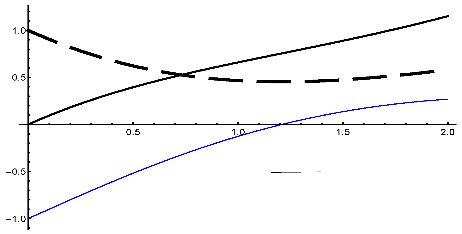
Example 1.

Consider the following FIVP:

$$y^{″}\left(t\right)+y^{\prime }\left(t\right)+y\left(t\right)=ty\left(0\right)=0,y^{\prime }\left(0\right)=1$$

(13)

Solution:

The analytical solution of this problem is $y\left(t\right)=exp\left(\frac{-t}{2}\right)(cos(\frac{\sqrt{3}t}{2}+\frac{1}{\sqrt{3}}sin\left(\frac{\sqrt{3}t}{2}\right)+t-1$. Before fuzzifying the differential equation, we first analyze the switching points of the solution function as mentioned in Section 3. For this purpose, the graph of the solution function and its first and second derivatives in Figure 1.

The graphs show that $f\left(t\right).f^{\prime }\left(t\right)>0$ and $f^{\prime }\left(t\right).f^{″}\left(t\right)<0$ for $t\in [0,1.204]$. This shows that f has differentiability of type-(i), $f^{\prime }$ has differentiability of type-(ii), and the second-order differential equation has the solution of the $D_{1,2}^2$ system. This solution is switched for $t\in (1.204,5]$, where $f\left(t\right).f^{\prime }\left(t\right)>0$ and $f^{\prime }\left(t\right).f^{″}\left(t\right)>0$, and the equation has the solution of type $D_{1,1}^2$ within the interval. This shows that the solution switches from type $D_{1,2}^2$ to $D_{1,1}^1$.

Now, the second-order differential equation is converted into a system of first-order differential equations. Differential Equation (13) is converted into a system of first-order differential equations, represented in Equation (14).

$$\begin{array}{ccc}{y}_1^{\prime }\left(t\right)\hfill & =& y_2\left(t\right)\hfill \\ y_2^{\prime }\left(t\right)\hfill & =& t-y_2\left(t\right)-y_1\left(t\right)\hfill \end{array}$$

(14)

The initial conditions also change to $y1\left(0\right)=0,y2\left(0\right)=1$. Replacing $t^{*}=t-t_i$, then above equation will become

$$\begin{array}{ccc}y{1}^{\prime }\left(t^{*}\right)\hfill & =& y_2\left(t^{*}\right)\hfill \\ y{2}^{\prime }\left(t^{*}\right)\hfill & =& t^{*}+t_i-y_2\left(t^{*}\right)-y_1\left(t^{*}\right)\hfill \end{array}$$

(15)

Every real number can be represented as the triangular fuzzy number. The initial values are fuzzified, and this problem becomes an FIVP. These values are represented as the interval-valued fuzzy set

$$y1(0,\gamma )={[\underline{y1},\overline{y1}]}_{\gamma }=[-1+\gamma ,1-\gamma ]$$

Similarly, the second value is fuzzified as

$$y2(0,\gamma )={[\underline{y2},\overline{y2}]}_{\gamma }=[-1+\gamma ,1-\gamma ]$$

The system of ODEs is converted into the equivalent system of ordinary differential equations with fuzzy initial value conditions. This process splits the system of ODEs into two equivalent systems of ODEs, and Equation (15) will become

$$\begin{array}{ccc}{\underline{y1}}^{\prime }(t^{*},\gamma )\hfill & =& \underline{y2}(t^{*},\gamma )\hfill \\ \overline{y{1}^{\prime }}(t^{*},\gamma )\hfill & =& \overline{y2}(t^{*},\gamma )\hfill \\ \underline{y{2}^{\prime }}(t^{*},\gamma )\hfill & =& t^{*}+t_i-\overline{y2}\left((t^{*},\gamma )\right)-\overline{y1}(t^{*},\gamma )\hfill \\ \overline{y{2}^{\prime }}(t^{*},\gamma )\hfill & =& t^{*}+t_i-\underline{y2}(t^{*},\gamma )-\underline{y1}(t^{*},\gamma )\hfill \end{array}$$

(16)

Taking the differential transformation of the above system of equations, we get the recurrence relation for this system of equations between the two grid points $t_i$ and $t_{i+1}$, represented as

$$\begin{array}{ccc}{\underline{Y1}}_i(k+1,\gamma )\hfill & =& {\underline{Y2}}_i(k,\gamma )/(k+1)\hfill \\ {\overline{Y1}}_i(k+1,\gamma )\hfill & =& {\overline{Y2}}_i(k,\gamma )/(k+1)\hfill \\ {\underline{Y2}}_i(k+1,\gamma )\hfill & =& \delta (k-1)+t_i-{\overline{Y2}}_i\left((k,\gamma )\right)-{\overline{Y1}}_i(k,\gamma )/(k+1)\hfill \\ {\overline{Y2}}_i(k+1,\gamma )\hfill & =& \delta (k-1)+t_i-{\underline{Y2}}_i(k,\gamma )-{\underline{Y1}}_i(k,\gamma )/(k+1)\hfill \end{array}$$

(17)

with initial conditions, we get ${\underline{Y1}}_0(0,\gamma )=-1+\gamma ;{\overline{Y1}}_0(0,\gamma )=1-\gamma$ and ${\underline{Y2}}_0(0,\gamma )=\gamma {\overline{Y2}}_0(0,\gamma )=2-\gamma$. The whole interval is divided into the subintervals, and switching points are checked at each partition point. The differential transformation coefficients are determined from the above set of equations, and the lower and upper solutions are developed for each subdomain separately using the differential transformation method of order 20, namely, $DT20$. The final value of the preceding subdomain is used as the initial value of the next subdomain. For example, at $t=0.2$, y(t) in the first subinterval will be $y{\left(t\right)}_{\gamma }=[1.1144\gamma -1.0204,1.2084-1.1144\gamma ]$ such that $\gamma \in [0,1]$. The results are compared in

Table 4. Comparison of solutions for multiple t and $\gamma =1$.

$\gamma$	0.2	0.4	0.6	0.8	1	1.2	1.4	1.6	1.8	2
$\underline{y}$	0.0940	0.1807	0.2622	0.3402	0.4167	0.6582	0.5687	0.5694	0.6490	0.7331
$\overline{y}$	0.0940	0.1807	0.2622	0.3403	0.4171	0.4923	0.6582	0.7346	0.8156	0.9028

, in which the computed solutions for the grid point 0 are shown for the changing fuzzification parameter γ.

The point $t=1.2$ is the switching point, where $\underline{y2}=0.7724,\overline{y2}=0.7551$. For the next input, the values are interchanged, i.e., the upper solution becomes the lower solution and the lower solution changes to the upper solution by applying the min and max operators.

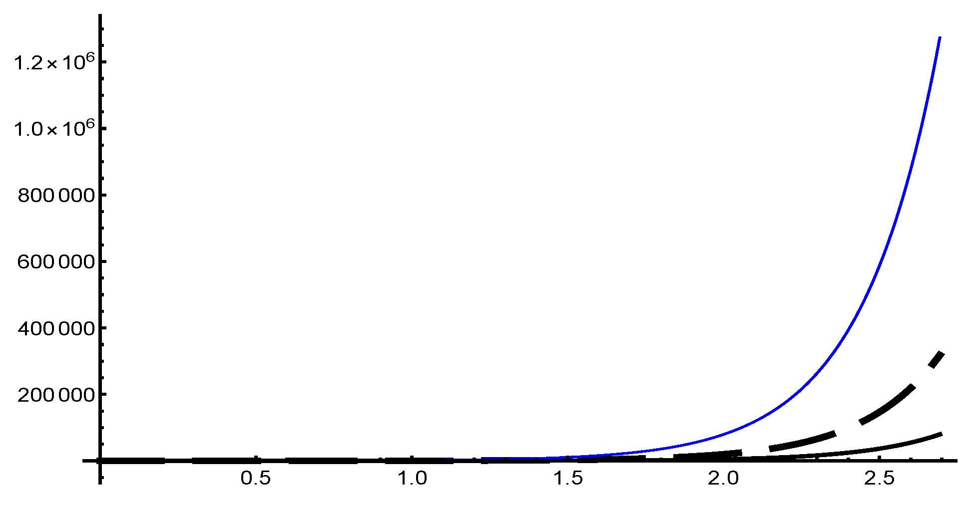
Example 2.

Consider the following FIVP:

$$y^{″}\left(t\right)-2y^{\prime }\left(t\right)-8y\left(t\right)=8t^2+20t+2t>0y\left(0\right)=0y^{\prime }\left(0\right)=8$$

(18)

over the interval $[0,3]$.

Solution:

The analytical solution of the problem is $y\left(t\right)=\frac{-5}{3}exp\left(-2t\right)+\frac{5}{3}exp\left(4t\right)-t^2-2t$.

In the first step, the domain of the analytic solution function is analyzed, and the Figure 2 of the solution function with its first and second derivatives is drawn. This graph shows that $f\left(t\right).f^{\prime }\left(t\right)>0$ for all $t\in [0,\infty ]$. As marked in Section 3, if f has a solution according to type-(i) derivatives, and if $f^{\prime }\left(t\right).f^{″}\left(t\right)>0$ for all $t\in [0,\infty ]$ as a result, then $f^{\prime }$ also has a derivative of type-(i). Thus, the problem has the $D_{1,1}^2$ solution in the $D_{m,n}$ system.

The solution of a second-order differential equation is determined by converting Differential Equation (18) into a system of first-order ODEs according to Equation (19).

$$\begin{array}{ccc}y{1}^{\prime }\left(t\right)\hfill & =& y2\left(t\right)\hfill \\ y{2}^{\prime }\left(t\right)\hfill & =& 2y2\left(t\right)+8y1\left(t\right)+8t^2+20t+2\hfill \end{array}$$

(19)

The initial conditions are also transferred according to the used transformation, $y_1\left(0\right)=0,y_2\left(0\right)=8$. Now, replacing $t^{*}=t-t_i$,

$$\begin{array}{ccc}y{1}^{\prime }\left(t^{*}\right)\hfill & =& y2\left(t^{*}\right)\hfill \\ y{2}^{\prime }\left(t^{*}\right)\hfill & =& 2y2\left(t^{*}\right)+8y1\left(t^{*}\right)+8{\left(t^{*}\right)}^2+8t_i^2+20t_i+2+(16t_i+20)\left(t^{*}\right)\hfill \end{array}$$

(20)

The differential transformation of this ODE system at grid point $t_i$ is computed as Equation (21).

$$\begin{array}{ccc}{\underline{Y1}}_i(k+1,\gamma )\hfill & =& {\underline{Y2}}_i(k,\gamma )/(k+1)\hfill \\ {\overline{Y1}}_i(k+1,\gamma )\hfill & =& {\overline{Y2}}_i(k,\gamma )/(k+1)\hfill \\ {\underline{Y2}}_i(k+1,\gamma )\hfill & =& 2[{\underline{Y2}}_i(k,\gamma )+8{\underline{Y1}}_i(k,\gamma )+8\delta (k-2)+(20+16t_i)\delta (k-1)+(8t_i^2+20t_i+2)\delta \left(k\right)]/(k+1)\hfill \\ {\overline{Y2}}_i(k+1,\gamma )\hfill & =& [2{\overline{Y2}}_i(k,\gamma )+8{\underline{Y1}}_i(k,\gamma )+8\delta (k-2)+(20+16t_i)\delta (k-1)+(8t_i^2+20t_i+2)\delta \left(k\right)]/(k+1)\hfill \end{array}$$

(21)

To solve the second-order initial value problem, the system of initial value problem is converted to the fuzzy initial value problem. For this, the initial conditions are fuzzified as $y1\left(0\right)=(-1+\gamma ,1-\gamma )$ and $y2\left(0\right)=(7+\gamma ,9-\gamma )$, and γ-level transformation of these initial conditions will be $\underline{Y1}(0,\gamma )=-1+\gamma ,\overline{Y1}(0,\gamma )=1-\gamma$ and $\underline{Y2}(0,\gamma )=7+\gamma \overline{Y2}(0,\gamma )=7+\gamma$. Similarly, the recurrence relation for the upper solution will be written as stated in Equation (21). The computed solution for multiple grid points is shown in

Table 5. Computation of solution at multiple grid points for $\gamma =1$.

$\gamma$	0.3	0.6	0.9	1.2	1.5	1.8	2.1	2.4
$\underline{y}$	1.6677	4.7970	11.0242	23.4867	48.2328	96.9402	192.1757	334.9335
$\overline{y}$	1.6677	4.7970	11.0243	23.4875	48.2340	293.8502	720.9583	1336

for $\gamma =1$.

The results show that there is no switching point, and the definition of the derivative is chosen according to the initial conditions.

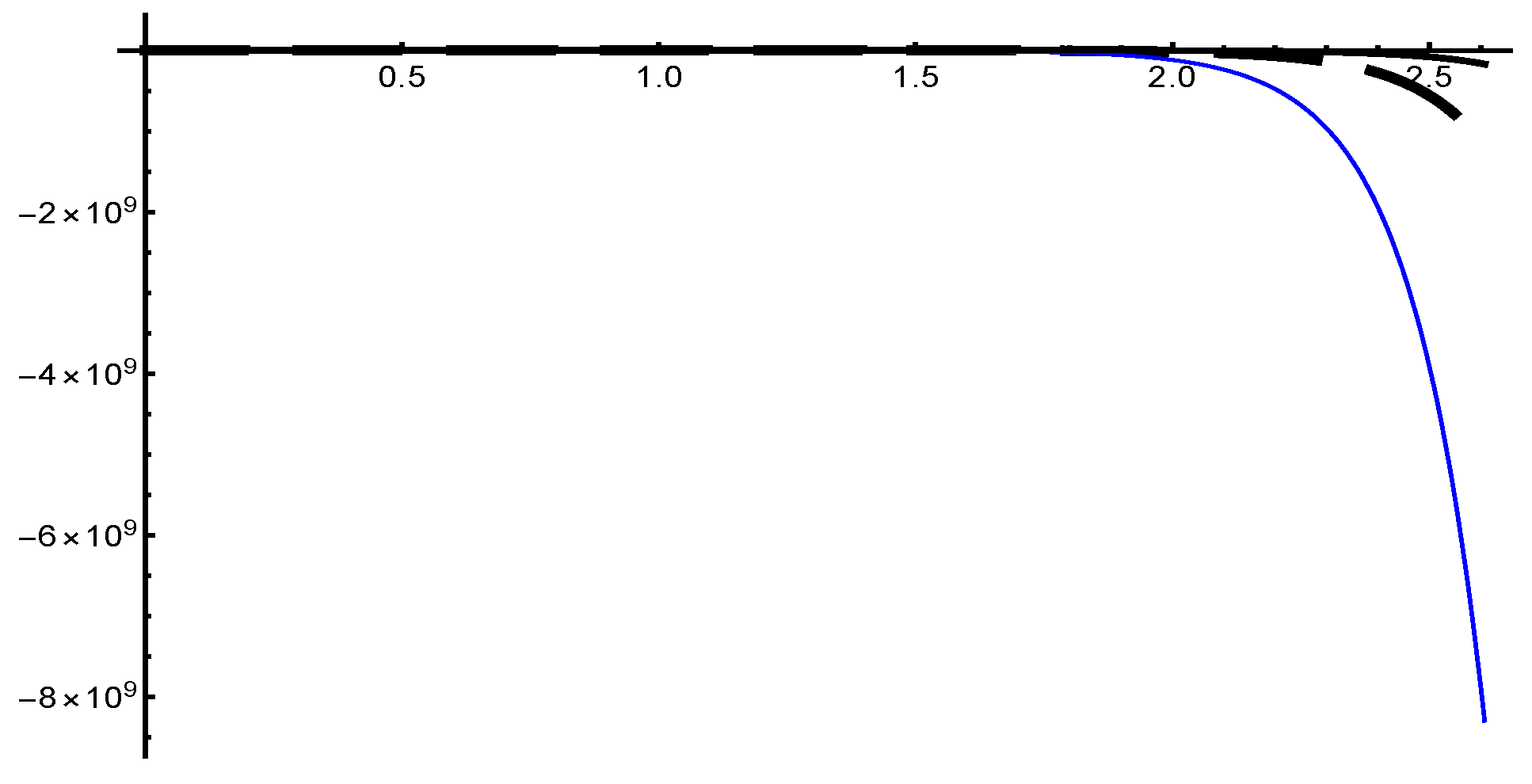
Example 3.

Consider the following FIVP:

$$y^{″}\left(t\right)-6y^{\prime }-7y\left(t\right)=-9e^{-2t}0\le t\le 2y\left(0\right)=-2,y^{\prime }\left(0\right)=-13$$

(22)

Solution:

$y\left(t\right)=e^{-t}-2e^{7t}-e^{-2t}$ is the analytical solution of Differential Equation (22).

The Figure 3 shows that the function and its first and second derivatives are always negative. This results in $f\left(t\right).f^{\prime }\left(t\right)>0$ for all $t\in [0,\infty ]$. As a result, f has a solution according to the type-(i) derivative, and $f^{\prime }\left(t\right).f^{″}\left(t\right)>0$ for all $t\in [0,\infty ]$; as a result, $f^{\prime }$ has a solution according to the type-(i) derivative, and the problem has the $D_{1,1}^2$ solution in the $D_{m,n}$ system.

For a numerical solution of a higher-order differential equation with fuzzy initial values, first convert Equation (22) in the system of first-order differential equations as Equation (23).

$$\begin{array}{ccc}y{1}^{\prime }\hfill & =& y2\hfill \\ y{2}^{\prime }\hfill & =& 6y2+7y1-9e^{-2t}\hfill \end{array}$$

(23)

The initial conditions become $y_1\left(0\right)=-2,y_2\left(0\right)=-13$. The system of initial value problem is converted to the fuzzy initial value problem, and these conditions become $y_1(0,\gamma )=(-3+\gamma ,-1-\gamma )$ and $y_2(0,\gamma )=(7+\gamma ,9-\gamma )$. The differential equation for the system between the two grid points $t_i$ and $t_{i+1}$ can be represented as Equation (24), the recurrence relation for the differential transform method:

$$\begin{array}{ccc}Y1(K+1)\hfill & =& Y2\left(K\right)\hfill \\ Y2(K+1)\hfill & =& 6Y2\left(k\right)+7Y1\left(k\right)-9\frac{{(-2)}^k}{k!}{e}^{2t_i}\hfill \end{array}$$

(24)

Now, for the fuzzy initial value solutions, the lower system of the recurrence relation can be written as Equation (25).

$$\begin{array}{ccc}{\underline{Y1}}_i(k+1,\gamma )\hfill & =& {\underline{Y2}}_i(k,\gamma )/(k+1)\hfill \\ {\underline{Y1}}_i(k+1,\gamma )\hfill & =& {\underline{Y2}}_i(k,\gamma )/(k+1)\hfill \\ {\underline{Y2}}_i(k+1,\gamma )\hfill & =& [6{\underline{Y2}}_i(k,\gamma )+7{\underline{Y1}}_i(k,\gamma )-9\frac{{(-2)}^k}{k!}{e}^{2t_i}]/(k+1)\hfill \\ {\underline{Y2}}_i(k+1,\gamma )\hfill & =& [6{\underline{Y2}}_i(k,\gamma )+7{\underline{Y1}}_i(k,\gamma )-9\frac{{(-2)}^k}{k!}{e}^{2t_i}/(k+1)\hfill \end{array}$$

(25)

The transformation of initial conditions yields ${\underline{Y1}}_0(0,\gamma )=-1+\gamma ,{\overline{Y1}}_0(0,\gamma )=1-\gamma$ and ${\underline{Y2}}_0(0,\gamma )=7+\gamma ,{\overline{Y2}}_0(0,\gamma )=9-\gamma$. The series solution is computed for the upper and lower approximation in each subdomain separately. The initial values at the point $t=0.9$ are the terminal values of the previous series, which is

$$\begin{array}{ccc}\underline{y1}\hfill & =& 2.1518\gamma +2.6452,\overline{y1}=6.9488-2.1518\gamma \hfill \\ \underline{y2}\hfill & =& 6.9108\gamma +19.1886,\overline{y2}=33.0103-6.91086\gamma \hfill \end{array}$$

(26)

A similar method is followed for other points, and the results are represented in

Table 6. Computation of lower and upper approximate solutions at multiple t for $\gamma =1$.

t	0	0.4	0.8	1.2	1.6	2
$\underline{y}$	−2	−27.0747	−425.7578	−6953.7e+03	−1.1424e+05	−1.9238e+06
$\overline{y}$	−2	−27.0747	−425.7578	−6953.7e+03	−1.1424e+05	−1.8331e+06

.

These results show that the solution has no switching point, and the system has $D_{1,1}^2$ differentiability in the domain.

6. Discussion

Second-order differential equations with fuzzy initial value problems are solved using a system of first-order differential equations. The second-order differential equation has four possible solutions in the $D_{n,m}^2$ system. In this paper, we discuss the switching points, which are the points where the definition of differentiability switches from type-(i) to type-(ii) or vice versa. These sorts of solutions are developed for second-order differential equations. It is shown that only one definition of differentiability is valid for one point or subinterval. This definition switches to the second definition at the switching point. Three numerical examples are solved using the min, max operators for switching points, and promising results validate the method. These solutions are important for the development of automatic solutions to modeling and simulation of problems.

7. Conclusions

In this paper, we develop the solution of a second-order fuzzy initial value problem with the analysis of switching points using the differential transformation method. The definition of fuzzy differentiability switches from type-(i) to type-(ii) and vice versa when the product of the function and its derivative changes signs within the domain of the function. These switching points are handled by applying the min, max operators. This demonstrates the single solution of an FIVP at time t or for the interval. This method is used to solve second-order differential equations by converting second-order ODEs into an equivalent system of first-order ODEs. Application of the min, max operators will be applied for solving higher-order differential equations with fuzzy initial values in future works.

References

1. Zadeh, L. Fuzzy sets. Inf. Control 1965, 8, 338–353. [Google Scholar] [CrossRef]
2. Chang, S.S.L.; Zadeh, L. On fuzzy mapping and control. IEEE Trans. Syst. Man Cybern. 1972, 2, 30–34. [Google Scholar] [CrossRef]
3. Dubois, D.; Prade, H. Towards fuzzy differential calculus: Part 3. differentiation. Fuzzy Sets Syst. 1982, 8, 225–233. [Google Scholar]
4. Geotschel, R.; Voxman, W. Elementary fuzzy calculus. Fuzzy Sets Syst. 1986, 18, 31–43. [Google Scholar]
5. Puri, M.L.; Ralescu, D.A. Differentials of fuzzy functions. J. Math. Anal. Appl. 1983, 91, 552–558. [Google Scholar] [CrossRef]
6. Fard, O.S.; Ghal-Eh, N. Numerical solutions for linear system of first-order fuzzy differential equations with fuzzy constant coefficients. Inf. Sci. 2011, 181, 4765–4779. [Google Scholar] [CrossRef]
7. Qiu, D.; Zhang, W. Symmetric fuzzy numbers and additive equivalence of fuzzy numbers. Soft Comput. 2013, 17, 1471–1477. [Google Scholar] [CrossRef]
8. Qiu, D.; Lu, C.; Zhang, W.; Lan, Y. Algebraic properties and topological properties of the quotient space of fuzzy numbers based on Mares equivalence relation. Fuzzy Sets Syst. 2014, 245, 63–82. [Google Scholar] [CrossRef]
9. Qiu, D.; Zhang, W.; Lu, C. On fuzzy differential equations in the quotient space of fuzzy numbers. Fuzzy Sets Syst. 2016, 295, 72–98. [Google Scholar] [CrossRef]
10. Ahmadi, M.B.; Kiania, N.A. Differential transformation method for solving fuzzy differential inclusions by fuzzy partitions. Int. J. Ind. Math. 2013, 5, 237–249. [Google Scholar]
11. Plotnikov, A.V.; Skripnik, N.V. Fuzzy Differential Equations with Generalized Derivative. J. Fuzzy Set Valued Anal. 2012, 2012, jfsva-00113. [Google Scholar] [CrossRef]
12. Bede, B.; Gal, S.G. Solutions of fuzzy differential equations based on generalized differentiability. Commun. Math. Anal. 2010, 9, 22–41. [Google Scholar]
13. Buckley, J.J.; Feuring, T. Fuzzy differential equations. Fuzzy Sets Syst. 2000, 110, 43–54. [Google Scholar]
14. Georgiou, D.; Nieto, J.J.; Rodriguez-Lopez, R. Initial value problems for higher-order fuzzy differential equations. Nonlinear Anal. Theory Methods Appl. 2005, 63, 587–600. [Google Scholar]
15. Bede, B.; Gal, S.G. Generalizations of the Differentiability of Fuzzy-number-valued Functions with Applications to Fuzzy Differential Equations. Fuzzy Sets Syst. 2005, 151, 581–599. [Google Scholar]
16. Effati, S.; Pakdaman, M. Artificial Neural Network Approach for Solving Fuzzy Differential Equations. Inf. Sci. 2010, 180, 1434–1457. [Google Scholar]
17. Jafari, H.; Saeidy, M.; Baleanu, D. The variational iteration method for solving n-th order fuzzy differential equations. Central Eur. J. Phys. 2012, 10, 76–85. [Google Scholar]
18. Babolian, E.; Sadeghi, H.; Javadi, S. Numerically Solution of Fuzzy Differential Equations by Adomian Method. Appl. Math. Comput. 2004, 149, 547–557. [Google Scholar]
19. Allahviranloo, T.; Ahmady, N.; Ahmady, E. Numerical solution of fuzzy differential equations by predictor-corrector method. Inf. Sci. 2007, 177, 1633–1647. [Google Scholar]
20. Allahviranloo, T.; Ahmady, E.; Ahmady, N. A method for solving nth order fuzzy linear differential equations. Int. J. Comput. Math. 2009, 86, 730–742. [Google Scholar]
21. Allahviranloo, T.; Shafiee, M.; Nejatbakhsh, Y. A Note on “Fuzzy Differential Equations and the Extension Principle”. Inf. Sci. 2009, 179, 2049–2051. [Google Scholar]
22. Ma, M.; Friedman, M.; Kandel, A. Numerical solutions of fuzzy differential equations. Fuzzy Sets Syst. 1999, 105, 133–138. [Google Scholar]
23. Allahviranloo, T.; Abbasbandy, S.; Salahshour, S.; Hakimzadeh, A. A New Method for Solving Fuzzy Linear Differential Equations. Computing 2011, 92, 181–197. [Google Scholar]
24. Allahviranloo, T.; Salahshour, S. Euler Method for Solving Hybrid Fuzzy Differential Equation. Soft Comput. 2011, 15, 1247–1253. [Google Scholar]
25. de Barros, L.C.; Pedro, F.S. Fuzzy differential equations with interactive derivative. Fuzzy Sets Syst. 2017, 309, 64–80. [Google Scholar] [CrossRef]
26. Isa, S.; Abdul Majid, Z.; Ismail, F.; Rabiei, F. Diagonally Implicit Multistep Block Method of Order Four for Solving Fuzzy Differential Equations Using Seikkala Derivatives. Symmetry 2018, 10, 42. [Google Scholar] [CrossRef]
27. Ahmadian, A.; Salahshour, S.; Chan, C.S.; Baleanu, D. Numerical solutions of fuzzy differential equations by an efficient Runge-Kutta method with generalized differentiability. Fuzzy Sets Syst. 2018, 331, 47–67. [Google Scholar] [CrossRef]
28. Allahviranloo, T.; Chehlabi, M. Solving Fuzzy Differential Equations Based on the Length Function Properties. Soft Comput. 2015, 19, 307–320. [Google Scholar]
29. Long, H.V.; Nieto, J.J.; Son, N.T.K. New approach for studying nonlocal problems related to differential systems and partial differential equations in generalized fuzzy metric spaces. Fuzzy Sets Syst. 2018, 331, 26–46. [Google Scholar] [CrossRef]
30. Zhang, D.; Feng, W.; Zhao, Y.; Qiu, J. Global existence of solutions for fuzzy second-order differential equations under generalized H-differentiability. Comput. Math. Appl. 2010, 60, 1548–1556. [Google Scholar] [CrossRef]
31. Rabiei, F.; Ismail, F.; Ahmadian, A.; Salahshour, S. Numerical Solution of Second-Order Fuzzy Differential Equation Using Improved Runge-Kutta Nystrom Method. Math. Probl. Eng. 2013, 2013, 803462. [Google Scholar]
32. Najariyan, M.; Mazandarani, M. A note on “Numerical solutions for linear system of first-order fuzzy differential equations with fuzzy constant coefficients”. Inf. Sci. 2015, 305, 93–96. [Google Scholar] [CrossRef]
33. Zhou, X. Differential Transformation and its Applications for Electric Circuits; Hauzhong University Press: Wuhan, China, 1986; Volume 24, pp. 1279–1289. [Google Scholar]
34. Mirzaee, F. Differential Transformation Method for Solving the Linear and Nonlinear Systems of Ordinary Differential Equations. Appl. Math. Sci. 2011, 5, 3465–3472. [Google Scholar]
35. Allahviranloo, T.; Kiani, N.; Motamedi, N. Solving fuzzy differential equations by differential transformation method. Inf. Sci. 2009, 179, 956–966. [Google Scholar]
36. Akin, O.; Khaniyev, T.; Oruç, O.; Türksen, I. An algorithm for the solution of second order fuzzy initial value problems. Expert Syst. Appl. 2013, 40, 953–957. [Google Scholar]
37. Guo, X.; Shang, D.; Lu, X. Fuzzy approximate solutions of second-order fuzzy linear boundary value problems. Bound. Value Probl. 2013, 2013, 212. [Google Scholar] [CrossRef]
38. Kadkhoda, N.; Roushan, S.S.; Jafari, H. Differential Transform Method: A Tool for Solving Fuzzy Differential Equations. Int. J. Appl. Comput. Math. 2017, 4, 33. [Google Scholar] [CrossRef]
39. Khastan, A.; Nieto, J.J. A boundary value problem for second order fuzzy differential equations. Nonlinear Anal. Theory Methods Appl. 2010, 72, 3583–3593. [Google Scholar] [CrossRef]
40. Kadak, U.; Ozluk, M. A new approach for the sequence spaces of fuzzy level sets with the partial metric. J. Fuzzy Set Valued Anal. 2014, 2014, 1–13. [Google Scholar] [CrossRef]
41. Khastan, A.; Bahrami, F.; Ivaz, K. New Results on Multiple Solutions for nth-Order Fuzzy Differential Equations under Generalized Differentiability. Bound. Value Probl. 2009, 2009, 395714. [Google Scholar] [CrossRef]
42. Bede, B.; Stefanini, L. Generalized differentiability of fuzzy-valued functions. Fuzzy Sets Syst. 2013, 230, 119–141. [Google Scholar]
43. Mansouri, S.S.; Ahmad, N. A Numerical Method For Solving Nth-Order Fuzzy Differential Equation by using Characterization Theorem. Commun. Numerical Anal. 2012, 2012, cna-00054. [Google Scholar] [CrossRef]
44. Allahviranloo, T.; Kiani, N.; Barkhordari, M. Toward the existence and uniqueness of solutions of second-order fuzzy differential equations. Inf. Sci. 2009, 179, 1207–1215. [Google Scholar]
45. Kadak, U.; Basar, F. Power series of fuzzy numbers with real or fuzzy coefficients. Filomat 2012, 26, 519–528. [Google Scholar]
Figure 1. Graph of the function and its first and second derivatives. The black line shows the function, the dashed line shows the first derivative, and the blue line shows the second derivative.
Mathematics 07 00231 g001
Figure 2. Graph of the function and its first and second derivatives. The black line shows the function, the dashed line shows the first derivative, and the blue line shows the second derivative.
Mathematics 07 00231 g002
Figure 3. Graph of the function and its first and second derivatives. The black line shows the function, the dashed line shows the first derivative, and the blue line shows the second derivative.
Mathematics 07 00231 g003