1. Introduction
In
, the concept of closed
k-surface was established in References [
1,
2] and its digital topological characterizations were also studied [
3,
4,
5,
6,
7]. Many explorations of various properties of closed
k-surfaces have been proceeded from the viewpoints of digital topology and digital geometry [
1,
2,
3,
4,
5,
6,
7,
8,
9]. Based on the studies of the earlier works [
3,
4,
5,
10,
11], given (digital) closed
k-surfaces and connected sums of closed
k-surfaces, we will investigate the fixed point property (
FPP) or the almost fixed point property (
AFPP) of them. Moreover, after explaining the Euler characteristic of a closed
k-surface in Reference [
5] more precisely, we confirm strong relationships between the Euler characteristic of a closed
k-surface and that of the continuous analog (or geometric realization) of a closed
k-surface.
Indeed, there are several kinds of approaches to establish a digital
k-surface [
3,
4,
5,
6,
12,
13]. In digital surface theory, we need to consider a binary digital image structure. To be precise, in the case of
, we often assume a digital image
X in the digital picture
P,
Thus, we can study a (digital) closed
k-surface with one of the above picture
P. Moreover, for a digital image
, the notion of the Euler characteristic of
was proposed in several ways [
3,
4,
5,
14,
15,
16,
17,
18,
19]. The concept of digital connected sum of closed
k-surfaces in
was firstly introduced in Reference [
3] by using several types of simple closed
k-curves in
.
Hereafter, we denote a simple closed k-surface in (for more details, see Definition 6) with . Indeed, given an , the studies of its Euler characteristic, an efficient formulation of a continuous analog of it, and the FPP for play important roles in digital geometry. Thus, we have the following queries:
- (Q1)
How to establish a geometric realization of an ?
- (Q2)
Does the geometric realization transform an into a certain spherical (or a sphere-like) polyhedron in ?
- (Q3)
How to define the Euler characteristic of an ?
- (Q4)
Are there certain relationships between the Euler characteristic of an and that of a geometric realization of an ?
- (Q5)
What about the FPP or the AFPP for an ?
To address these issues, Reference [
5] introduced the Euler characteristic of an
, which can facilitate the studies of both digital and typical surface theories. This paper continues a series of studies of Euler characteristics of digital surfaces [
5]. In order to prevent a certain misunderstanding or wrong interpretation of the Euler characteristic of an
, after referring to several essential notions associated with the Euler characteristic of an
, the present paper corrects some assertions in Reference [
14] involving the Euler characteristics of an
and a connected sum of closed
k-surfaces. To be precise, we will more precisely explain how to define the Euler characteristics of an
already introduced in Reference [
5] and a digital connected sum introduced in Reference [
3]. Indeed, the Euler characteristic of an
suggested in Reference [
5] is proved to be consistent with the typical Euler characteristic of a closed surface from the viewpoints of algebraic topology and polyhedral geometry.
The rest of the paper is organized as follows:
Section 2 refers to some notions involving a digital
k-surface and a connected sum of two digital
k-surfaces. Moreover, it confirms the pointed 18-contractibility of
which will be used in the paper.
Section 3 establishes the sets
and
(see Definitions 8 and 9) to develop a 2-dimensional simplicial complex as a geometric realization of a simple closed
k-surface
.
Section 4 studies the Euler characteristics of a closed
k-surface and a connected sum of two closed
k-surfaces proposed in Reference [
5]. In particular, given an
, using the set
, we can characterize the Euler characteristic of an
.
Section 5 studies the
FPP or the
AFPP for several kinds of simple closed
k-surfaces in
,
,
,
, and so on. Finally, we prove that the simple closed 18-surfaces
and
do not have the
AFPP. Hence, we conclude that, in digital topology, the triviality or the non-triviality of the Euler characteristics of simple closed
k-surfaces are irrelevant to the
FPP or the
AFPP. Furthermore, we corrects many errors in the paper written by Boxer et al. in Reference [
14] (see Remarks 11 and 12) and some mistakes in Reference [
3,
4] (see Remark 10).
Section 6 concludes the paper with some remarks.
2. Basic Notions Related to Digital -Surfaces and a Connected Sum for -Surfaces
In order to make the paper self-contained, let us now recall some terminology from digital curve and digital surface theories. Let and represent the sets of natural numbers and integers, respectively.
Rosenfeld [
20] called a set
with a
k-adjacency a digital image, denoted by
. In particular, in digital surface theory, let us consider a binary digital image
with a
k-adjacency in a digital picture
[
17,
20], where
. Then, we call the pair
a digital image with a
k-adjacency (for short,
digital image). In order to study
in
, we need
k-adjacency relations of
which are generalizations of the commonly used 4- and 8-adjacency of
, and 6-, 18-, and 26-adjacency of
. To be precise, we will say that distinct points
are
k-(or
-)adjacent if they satisfy the following property [
10] (for more details, see also Reference [
21] as an advanced representation of the
k-adjacency relations of
in Reference [
10]):
For a natural number
t,
, we say that distinct points
are
-(
k-, for short)adjacent if at most
t of their coordinates differs by
and all others coincide.
Concretely, these
-adjacency relations of
are determined according to the number
[
10] (see also Reference [
21]). In the present paper, we will use the symbol “
” to introduce new notions without proving the fact.
Using the operator of Equation (2), the
k-adjacency relations of
are obtained [
10] (see also References [
21,
22]), as follows
A digital image
in
can indeed be considered to be a set
with the
k-adjacency relation of Equation (3). Using the
k-adjacency relations of
of Equation (3), we say that a digital
k-neighborhood of
p in
is the set [
20]
Furthermore, we often use the notation [
17]
For
with
, the set
with 2-adjacency is called a digital interval [
17].
Let us now recall some terminology and notions which are used in this paper.
We say that two subsets
and
of
are
k-adjacent if
and that there are points
and
such that
a and
b are
k-adjacent [
17]. In particular, in case
B is a singleton, say
, we say that
A is
k-adjacent to
x.
For a
k-adjacency relation of
, a
k-path with
elements in
is assumed to be a finite sequence
such that
and
are
k-adjacent if
[
17].
A digital image is said to be k-connected if, for any distinct points such as in , there is a k-path such that and .
For a digital image , the k-component of is defined to be the largest k-connected subset of containing the point x.
We say that a simple
k-path is a finite set
such that
and
are
k-adjacent if and only if
[
17]. In the cases
and
, we denote the length of the simple
k-path with
.
A simple closed
k-curve (or simple
k-cycle) with
l elements in
[
10], denoted by
,
is the set of even natural numbers [
10,
17] and is the finite set
such that
and
are
k-adjacent if and only if
[
10].
For a digital image
, a digital
k-neighborhood of
with radius
is defined in
X as the following subset [
10] of
X:
where
is the length of a shortest simple
k-path from
to
x and
. For instance, for
, we obtain [
10]
Rosenfeld [
20] defined the notion of digital continuity of a map
by saying that
f maps every
-connected subset of
into a
-connected subset of
.
Motivated by the digital continuity proposed by Rosenfeld, in terms of the digital
k-neighborhood of a point with radius 1 (see Equation (5)), the digital continuity of a map between digital images was represented, as follows:
Proposition 1 ([
10,
11])
. Let and be digital images in and , respectively. A function is (digitally) -continuous if and only if, for every , . In Proposition 1 in case
and
, the map
f is called a
k-continuous map. Since an
n-dimensional digital image
is considered to be a set
X in
with one of the
k-adjacency relations of Equation (3) (or a digital
k-graph [
23]), regarding a classification of
n-dimensional digital images, we use the term a
-isomorphism (or
k-isomorphism) as in Reference [
23] (see also Reference [
11]) rather than a
-homeomorphism (or
k-homeomorphism) as in Reference [
24].
Definition 1 ([
23] (see also a
-homeomorphism in Reference [
24]))
. Consider two digital images and in and , respectively. Then, a map is called a -isomorphism if h is a -continuous bijection, and further, is -continuous. Then, we use the notation . Moreover, in the case , we use the notation . In References [
23,
25,
26], we developed many notions from the viewpoint of digital graph theory, such as graph
-homomorphism, graph
-isomorphism, and graph
-homotopy which are, respectively, digital graphical versions of the
-continuity,
-homeomorphism, and
-homotopy in digital topology. Since a digital image
can be recognized as a digital
k-graph [
5,
23], we mainly use the digital
k-graphical method to study Euler characteristics of a closed
k-surface in this paper.
The following notion of interior is often used in establishing the notion of digital connected sum.
Definition 2 ([
3])
. Let be a closed k-curve in . A point x of , the complement of in , is said to be interior to if it belongs to the bounded -connected component of . The following digital images
,
, and
[
3,
4,
10] play important roles in establishing a connected sum and in studying the digital fundamental group of a digital connected sum of closed
k-surfaces. Thus, we will recall them.
[
4], where
is a digital image 8-isomorphic to the digital image, i.e.,
;
[
4], where
is a digital image 4-isomorphic to the digital image, i.e.,
; and
[
4], where
is a digital image 8-isomorphic to the digital image, i.e.,
.
Based on the pointed digital homotopy in Reference [
27] (see also Reference [
24]), the following notion of
k-homotopy relative to a subset
is often used in studying
k-homotopic properties of digital images
in
. For a digital image
and
, we often call
a digital image pair.
Definition 3 ([
10] (see also [
3]))
. Let and be a digital image pair and a digital image, respectively. Let be -continuous functions. Suppose there exist and a function such thatfor all and ;
for all , the induced function given by for all is -continuous;
for all , the induced function given by for all is -continuous. Then, we say that H is a -homotopy between f and g [24]. Furthermore, for all , assume that the induced map on A is a constant which follows the prescribed function from A to Y. To be precise, for all and for all .
Then, we call H a -homotopy relative to A between f and g and we say that f and g are -homotopic relative to A in Y, in symbols.
In Definition 3, if
, then we say that
F is a pointed
-homotopy at
[
24]. When
f and
g are pointed
-homotopic in
Y, we use the notation
. In the cases
and
,
f and
g are said to be pointed
k-homotopic in
Y and we use the notations
and
, which denote the
k-homotopy class of
g. If, for some
,
is
k-homotopic to the constant map in the space
relative to
, then we say that
is pointed
k-contractible [
24]. The notion of digital homotopy equivalence was firstly introduced in Reference [
25] (see also Reference [
26]), as follows:
Definition 4 ([
25] (see also Reference [
26]))
. For two digital images and in , if there are k-continuous maps and such that the composite is k-homotopic to and the composite is k-homotopic to , then the map is called a k-homotopy equivalence and is denoted by . Moreover, we say that is k-homotopy equivalent to . Using the concept of digital
k-homotopy equivalence, we can classify digital images [
25]. Now, we recall the notion of
k-contractibility to be used later in this paper.
Definition 5 ([
10,
24,
27])
. For a digital image , if the identity map is k-homotopic relative to in X to a constant map with image consisting of some point , then is said to be pointed k-contractible. The following are proven in References [
3,
5,
10,
11,
24].
In case
X is pointed
k-contractible, the
k-fundamental group
is trivial [
24].
is not 8-contractible and
is not 4-contractible either [
3,
10].
are 8-contractible [
3,
5,
24].
Owing to the digital
-covering theory in References [
10,
11], the
k-fundamental groups of
were proven such that
is an infinite cyclic group [
10,
11].
Motivated by the calculation of the digital
k-fundamental group of
, i.e.,
in References [
10,
11], it turns out that
is not
k-contractible if
.
In particular, both the non-8-contractibility of and the non-4-contractibility of play important roles in formulating a connected sum of two closed k-surfaces.
In order to study a closed
k-surface in
, let us recall some terminology, such as a
k-corner, a generalized simple closed
k-curve, and so on. A point
is called a
k-corner if
x is
k-adjacent to two and only two points
y and
such that
y and
z are
k-adjacent to each other [
2]. The
k-corner
x is called
simple if
y and
z are not
k-corners and if
x is the only point
k-adjacent to both
y and
z.
is called a
generalized simple closed k-curve if what is obtained by removing all simple
k-corners of
X is a simple closed
k-curve [
2,
6]. For a
k-connected digital image
in
, we recall
where
and
are 26-adjacent} [
1,
2]. In general, for a
k-connected digital image
in
, we can state [
5]
where
Hereafter, for a
k-surface in
[
3,
4], we call the set
of Equation (7) the
minimal -adjacency neighborhood of
x in
X.
Reference [
5] introduced the notion of a closed
k-surface in
. However, in the present paper, we will stress the study of closed
k-surfaces in
with the following approach in References [
6,
7].
Definition 6 ([
3,
7])
. Let be a digital image in , and . Then, X is called a closed k-surface if it satisfies the following:- (1)
In case ,
- (a)
for each point , has exactly one k-component k-adjacent to x;
- (b)
has exactly two -components -adjacent to x; we denote by and these two components; and
- (c)
for any point (or in ), and . Furthermore, if a closed k-surface X does not have a simple k-point, then X is called simple.
- (2)
In case ,
- (a)
X is k-connected,
- (b)
for each point , is a generalized simple closed k-curve. Furthermore, if the image is a simple closed k-curve, then the closed k-surface X is called simple.
From now on, we denote a closed
k-surface in
with
,
, which will be used in this paper. Namely, we will consider only simple closed
k-surface in
in the picture as referred to in Equation (1), i.e.,
Definition 7 ([
3])
. In , let (resp. ) be a closed -(resp. a closed -)surface, where .Consider and take , where , , or and, further, , , or , respectively.
Let be a -isomorphism. Remove and from and , respectively.
Identify and by using the -isomorphism f. Then, the quotient space is obtained by for and is denoted by , where , , and the map is the inclusion map.
Owing to Definition 7,
is obtained in
. Moreover, the digital topological type of
absolutely depends on the choice of the subset
[
5]. Furthermore, the
k-adjacency of
is required as follows:
Remark 1 ([
3])
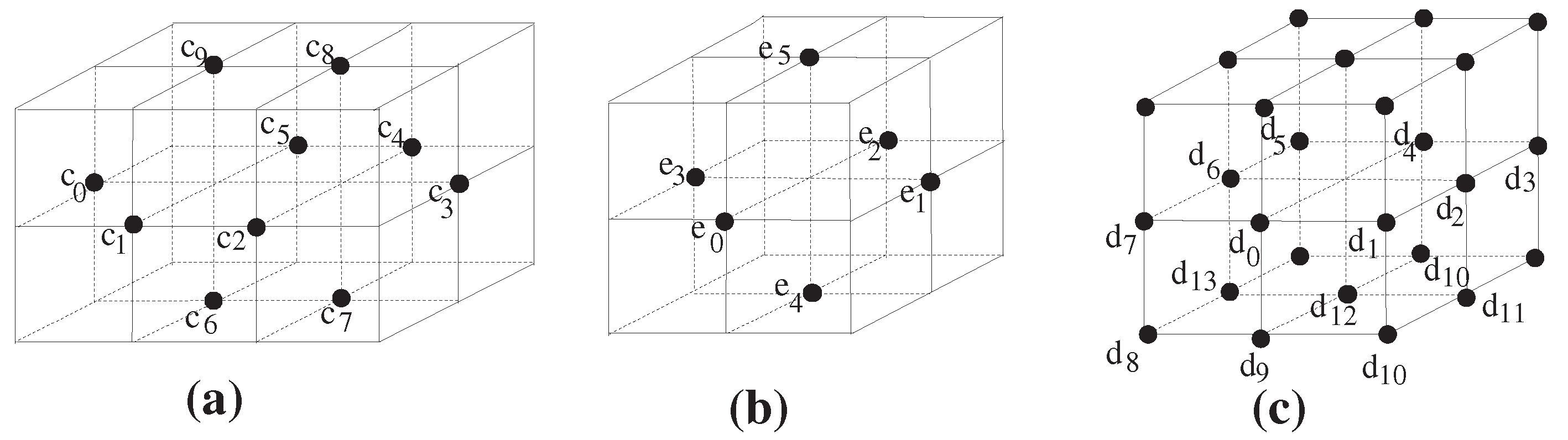
. In the quotient space , the subsets and in are assumed to be disjoint and are not k-adjacent, where . Then, the digital image is called a (digital) connected sum of and . Hereafter, we denote by
a
minimal simple closed k-surface in
(see
Figure 1). Furthermore, we recall the following closed
k-surfaces,
[
3]:
[
3,
4].
Then,
is the minimal simple closed 6-surface which is not 6-contractible (see
Figure 1c). Namely, we obtain
according to Equation (1).
Let us now recall two types of simple closed 18-surfaces which are pointed 18-contractible, e.g., and , as follows:
[
3,
4].
Then, Reference [
3,
4] stated that
is 18-contractible and that it is the minimal simple closed 18-surface (see
Figure 1b), i.e., we obtain
. Here, the term “minimal” comes from the minimal cardinality of the given digital image as a closed 18-surface.
In order to use the pointed 18-contractibility of
in this paper, we prove it more precisely, as follows:
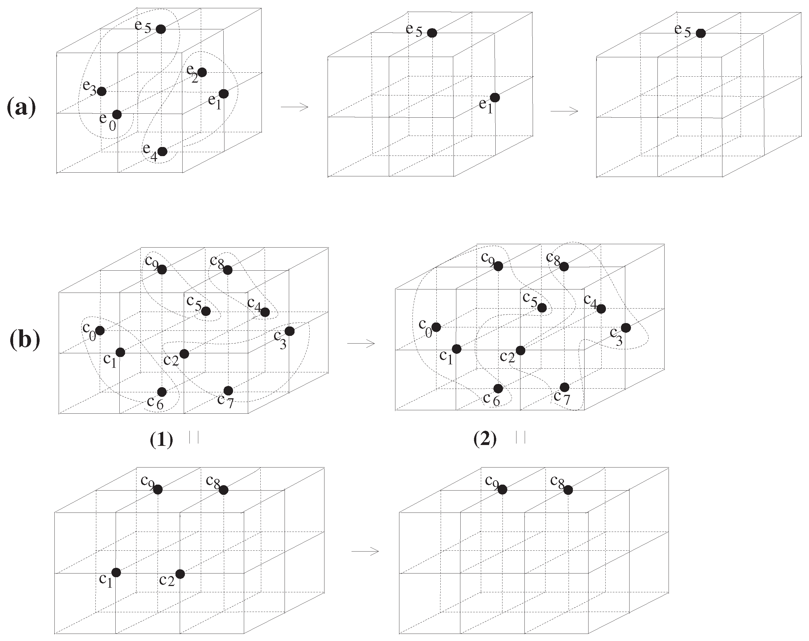
Lemma 1. is pointed 18-contractible.
Proof. Consider the map
(see
Figure 2a) such that
Then, the map H is an 18-homotopy relative to the set since it satisfies the following:
- (1)
for all as an identity map on the set , say , and as the constant map at the set
- (2)
for all , the induced function given by for all is -continuous;
- (3)
for all , the induced function given by for all is 18-continuous.
Thus, we obtain H which is an 18-homotopy between and .
- (4)
Furthermore, for all , assume that the induced map on is a constant.
Owing to properties (1)–(4), we prove that is 18-homotopy equivalent to and we complete the proof. □
In view of the proof of Lemma 1, although we proved the 18-contractibility of relative to the set , we find that is indeed 18-homotopy equivalent to any singleton .
Let us further introduce two simple closed k-surface, , as follows:
[
3,
4].
Then,
is indeed pointed 18-contractible (correction of the “
non-18-contractibility” of
in Theorem 4.3(3) of Reference [
3] and Theorem 4.2(3) of Reference [
4]). Moreover, it is proved to be a simple closed 18-surface (see
Figure 1a) [
3,
4]. Using a method similar to the 18-homotopy of Equation (8), we observe that there is indeed an 18-homotopy relative to the set
between
and
, which is the constant map at
(see
Figure 2b),
which implies the pointed 18-contractibility of
. More precisely, starting with
as the identity map
,
Figure 2(b1) shows the process of
and
Figure 2(b2) explains the process of
. Moreover,
means the constant map
. In addition, we observe that
is indeed 18-homotopy equivalent to any singleton
. Furthermore, Reference [
3] also already proved that
is simply 18-connected [
4].
, which is 26-contractible [
3,
4] and is the minimal simple closed 26-surface (see
Figure 1b). Finally, we obtain
according to Equation (1). Moreover, the proof of the 26-contractibility of
is trivially proceeded with the homotopy in Equation (8).
Indeed, we point out that the digital 6-, 18-, and 26-sphere-like models
, and
in
Figure 1 were firstly introduced in References [
3,
4].
Remark 2. Let T be the set , where . Then, we obtain the following:
- (1)
the digital image is not a closed 6-surface.
- (2)
is pointed 6-contractible.
Proof. (1) For any point , the set does not satisfy the properties Definition 6(1) (b) and (c).
(2) Using a method similar to the homotopy of Equation (8), we observe that there is a 6-homotopy relative to any singleton between the identity map and the constant map . Thus, we can conclude that is pointed 6-contractible relative to any singleton . □
3. A Geometric Realization of a Simple Closed -Surface
In order to address questions (Q1) and (Q2) in
Section 1, given an
and for each point
, we need to establish a special kind neighborhood of
x matching an open neighborhood of a certain point of a typical surface (or a 2-dimensional topological manifold). Indeed, given a digital image
in
, for each point
, the set
(see Equation (6)) plays an important role in examining if
is a simple closed
k-surface in
(see Definition 6). This approach is quite different from one examining if a topological space becomes a typical surface from the viewpoint of manifold theory. However, motivations of the two approaches are similar to each other. Roughly saying, each point
x of a 2-dimensional topological manifold (or a surface)
has an open neighborhood in
which is homeomorphic to an open disc in the 2-dimensional Euclidian topological space
. In digital surface theory, we also follow this kind of approach under a certain digital situation.
In order to study the Euler characteristics of a simple closed
k-surface and a connected sum of two simple closed
k-surfaces (see Reference [
5]), let us now recall a geometric realization of a digital image
. For a digital image
and each point
, owing to the set
, a special kind of geometric realization can be considered. However, in digital surface theory, we have some difficulties in establishing the so-called ‘
digital k-neighborhood of a point’ in
matching an open neighborhood of a point in a typical surface. Thus, motivated by the fact that, for an
and
, we observe that
is an essentially important set guaranteeing the closed
k-surface structure of the
(see also Remarks 5 and 6). Motivated by this observation, let us now treat this issue with a special kind of idea overcoming the difficulties. Roughly saying in advance, given a simple closed
k-surface
in
, consider it as a digital
k-graph, denoted by
. First of all, let us take all minimal
k-cycles in
denoted by
(see Definition 8). Hereafter, we need to remind that the set of Equation (10) is the set
in
. Next, we formulate a certain 2-dimensional simplicial complex in the 3-dimensional real space,
, say
, inherited from
(see Definition 9). More precisely, each 2-dimensional simplex in
is a polygon in
formulated by the corresponding minimal
k-cycle in
(see Definitions 8 and 9). Consequently, we have a geometric realization of
, denoted by
, which is the union of all
(see Definition 10). Then, we can observe that
is indeed a closed 2-dimensional simplicial complex, i.e., a sphere-like polygon in
(see Proposition 2).
Since the present paper focuses on the study of several types of connected sums of the simple closed k-surfaces , , and , hereafter, we only deal with simple closed k-surfaces in , denoted by . As mentioned above, given an , let us now propose the sets (see Definition 8) and (see Definition 9) derived by the set .
Definition 8. Given a simple closed k-surface in , for , let The set
has its own features, as follows:
Remark 3. (1) Each of the minimal k-cycles in , say , associated with Equation (11) need not be a simple closed k-cycle in (see the 18-curve consisting of of in Figure 3a). (2) The term “minimal” comes from the ‘minimal k-cycles’ in taken from the only one of the eight digital cubeswhere . (3) The element in need not contain the point x (see Example 1(3)).
(4) Not every k-cycle in is (see Example 1).
(5) may contain several k-cycles with different types depending on the situation (see Example 1).
Example 1. (1) In , for the point in in Figure 3a, we have as the set consisting of four 18-cycles, (2) In , for the point in in Figure 3b, we obtain as the set being composed of four 18-cycles, (3) In , for the point in Figure 3c, we have as the set consisting of twelve 6-cycles with four elements, Indeed, using each minimal
k-cycle in
, we can produce a certain polygon (a solid triangle or a solid rectangle) in
. For instance, in Example 1(a)(1), the given 18-cycle
produces a solid triangle, say
, and further, the 18-cycle
leads to a solid rectangle, say
in
. Motivated by this approach, we can define the following:
Definition 9. Given a simple closed k-surface in , for a point , letwhere means the polygon formulated by the minimal k-cycle . Indeed, is the set as the union of polygons (solid triangles or solid rectangles) formulated by the minimal k-cycles in . Then, we say that is a geometric realization of . In Definition 9, we observe that each minimal k-cycle in produces only a polygon as a subset of in . Thus, it turns out that is a simplicial complex inherited from (see Example 2).
Owing to the definition of
, for an
in
, it is obvious that the set
consists of triangles or rectangles with boundary in the subspace
, where
is the subspace topology induced by the 3-dimensional Euclidean topological space
. For instance, based on the set
in
Figure 3, we obtain the following:
Example 2. Depending on the points x in , (or ), or , according to in Figure 3, we have , as follows: - (1)
Based on , we observe that is the set as the union of polygons formulated by the 18-cycles in , i.e., the union of the two triangles with boundary generated by the two 18-cycles and and the two rectangles with boundary formulated by the 18-cycles and .
- (2)
Based on , we observe that is the set which is the union of four triangles with boundary formulated by four 18-cycles in .
- (3)
In terms of the methods used in Equations (1) and (2), based on , we observe that is the set as the union of twelve polygons (or regular rectangles) formulated by the twelve 6-cycles in .
Given an
, using
, let us now establish a geometric realization of
, as follows:
Definition 10. Given a simple closed k-surface in , letThen, we call the set the geometric realization of . Proposition 2. Given a simple closed k-surface in , the geometric realization is uniquely determined as a connected 2-dimensional simplicial complex (or a sphere-like polyhedron) in .
Proof. Given a simple closed k-surface in , for each point , it is obvious that the set is a simplicial complex consisting of triangles or rectangles with boundaries.
For two
k-adjacent points
and
in
,
and
have a non-empty intersection, i.e.,
which implies that
is connected. To be precise, the intersection
of Equation (13) is the union of the 2-dimensional simplexes (or polygons) derived from the minimal
k-cycles in
Namely, we observe the identity
Thus,
has some 2-dimensional simplexes (or polygons) in common from each of them. Since
is
k-connected, for any two
k-adjacent points in
, using the property of Equation (13), we can formulate a connected 2-dimensional simplicial complex because
is a 2-dimensional simplicial complex (see Definition 9), as follows
from the given
according to Definition 9. To be precise,
has 0-dimensional simplexes derived from each of all elements in
. The 1-dimensional simplexes of
are all line segments formulated by all two
k-adjacent points in
. Finally, the 2-dimensional simplexes of
come from the polygons in
. Obviously, owing to the definition of
and the notion of
(see Definition 6), there is no
n-dimensional simplex in
. □
According to Proposition 2, we obtain the following:
Remark 4. Given a simple closed k-surface in , , the geometric realization is a sphere-like polyhedron in .
Eventually, given an
,
is obtained in terms of the following process.
The term “generated” (see Definition 12 of Reference [
5]) in Reference [
5] means the process in Equation (14).
Remark 5. In view of Definitions 9 and 10, we observe that, given an and a point , the set can be considered a open neighborhood of x in , where the term as “Int” means the interior operator in the subspace , where is the subspace topology on induced by the 3-dimensional Euclidean topological space . This approach can facilitate the study of some objects in digital surface theory.
Remark 6 (Importance of the sets and with respect to a geometric realization of an ). Unlike a typical surface (or a 2-dimensional topological manifold) in the Euclidean topological space , we observe that, given an and motivated by the set, , the sets and play important roles in establishing a geometric realization of the given .
Owing to Proposition 2 and the process of Equation (14), given an in , we obtain (see Equation (13)) as a typical polyhedron without boundary in the subspace (see Remark 4).
Example 3. For in Figure 1a, we see that seems like to be a small rugby ball. 4. Euler Characteristics for Digital -Surfaces and Connected Sums of Closed -Surfaces
In order to address questions (Q3) and (Q4) in
Section 1 and, further, to exactly understand the notion of Euler characteristic of a simple closed
k-surface
in
(see Reference [
5]), we now stress that the geometric realization of
,
, is a sphere-like 2-dimensional simplicial complex generated by the set
(see Proposition 2).
Given an
in
, a ‘
2-dimensional digital k-simplex’ in
is obviously defined as the set
contained in
(see Equation (5)) such that each of two elements of
are
k-adjacent (see Reference [
23]). Moreover, a ‘
2-dimensional k-simplex’ in
is said to be a solid triangle formulated by a “2-dimensional digital
k-simplex”. Then, we can recognize some differences between a 2-dimensional digital
k-simplex (
resp. a 2-dimensional
k-simplex) and an element of
(
resp. ), as follows:
Remark 7. Given an , not every element of becomes a 2-dimensional digital k-simplex in .
Proof. Consider
in
Figure 3a. Whereas the set
contains the minimal 18-cycle
in
(see
Figure 3a), the 18-cycle
is not a 2-dimensional digital 18-simplex in
. □
Based on the
in
Figure 3a, we observe that, although the set
contains a rectangle (or a polygon), say
, generated by the minimal 18-cycle
in
, the rectangle
in
is not formulated by any 2-dimensional digital 18-simplex in
.
Example 4. For the simple closed 18-surface in Figure 1a, we have twelve polygons in generated by the set consisting of the following 18-cycles in However, in , we have only eight 2-dimensional digital 18-simplices, such as Thus, the simplicial complex generated by the eight 2-dimensional 18-simplex is quite different from the geometric realization of [5] (or the current geometric realization ). Remark 8 (Limitations of the approach of an Euler characteristic in Reference [
14])
. Given an referred to in Example 4, Reference [14] considered only the simplicial complexes formulated by only 2-dimensional digital k-simplexes on . Then, given an in , it is obvious that it need not produce a polyhedron in . To be precise, according to the approach of Reference [14], since each of the setsis not a 2-dimensional digital 18-simplex, the simplicial simplex induced by the 2-dimensional 18-simplices in is not even a polyhedron in .For instance, suppose the set generated by only the 2-dimensional 18-simplices in Reference [14] Then, the union of all polygons inherited from these eight 18-cycles is not a polyhedron in . This implies that, given an , the geometric approximation referred to in Reference [14] does not support a transformation from to a certain sphere-like polyhedron in . Hence, comparing Definition 10, the approach of Reference [14] is very restrictive. Hence, the current notions of and in Definitions 8 and 9 are substantially required in digital surface theory.
Using both the digital
k-graph theoretical method in References [
4,
10] and the notions of
and
, inherited from
(see Definitions 8 and 10 of the present paper), we can define the Euler characteristic of an
. Owing to Definition 10 and Proposition 2, we can make the definition for Euler characteristic of
in Reference [
5] clear in the following way.
Definition 11 ([
5])
. For an , the Euler characteristic of is defined bywhere and V means the number of the vertexes of , E is the number of the k-edges of , and F is the number of the polygons in . Remark 9 (Advantages of the approach of the current Euler characteristic of an
(see also Reference [
5])
. The approach using Definition 11 is consistent with the research of the Euler characteristic of a typical closed surface from algebraic topology and polyhedron geometry. Namely, for simple closed
k-surfaces in
, the following assertion in Reference [
5] is right with the same proof as in Reference [
5] according to the Definition 11 and Proposition 2.
Proposition 3. Given an , we obtain .
Proof. Using Proposition 2, given an , since is a sphere-like polyhedron in , we obtain . □
Example 5. (1) .
(2) .
Owing to Proposition 2, the digital analogue of the Euler characteristic of a connected sum in typical topology in References [
28,
29] was developed. Indeed, in Reference [
3], we stated the simple closed
k-surface structure of a connected sum of two simple closed
k-surfaces (see Theorem 5.4 of Reference [
3]). However, in order to use this fact in the present paper, we need to prove it more precisely, as follows:
Theorem 1. Given two simple closed k-surfaces and , is a simple closed k-surface in .
Proof. (Case 1) In the case
, we observe that, for each point
,
has exactly one
k-component
k-adjacent to
x. Moreover,
has exactly two
-components
-adjacent to
x. We denote these two components with
and
. Finally, for any point
(or
in
), we obtain
Since
does not have any simple
k-point,
is a simple closed
k-surface.
(Case 2) In the case , is obviously k-connected. Moreover, for each point , in view of the process of (see Definition 7 and Remark 1), is exactly a simple closed k-curve, which is a simple closed k-surface. □
Using Definition 11 and Theorem 1, as roughly proved in Reference [
3], we obtain the following:
Corollary 1. (1) [4]. (2) .
Proof. Owing to Theorem 1, the proofs of Equations (1) and (2) are completed. □
In view of Corollary 1, it turns out that the calculations of the Euler characteristics of connected sums of simple closed
k-surfaces suggested in Reference [
5] obviously hold, as follows:
Example 6. (1) .
(2) .
(3) .
In digital surface theory, Reference [
5] already proved that
is simply 18-connected. However, we now need to correct some errors in Reference [
5] relating to the calculations of the digital 6-fundamental groups of
and
in Reference [
4]. Indeed, using trivial extensions in Reference [
24], the calculations should be proceeded, as follows:
Remark 10. (1) The 18-fundamental group of should be calculated as a trivial group as in Reference [14] instead of the free group generated by two cyclic groups (correction of Lemma 3.3(3) of Reference [5]). (2) The 6-fundamental group of should be calculated as a trivial group as in Reference [14] instead of the free group generated by two cyclic groups (correction of Theorem 3.4(1) of Reference [5]). 5. The (Almost) Fixed Point Property for Digital -Surfaces and Connected Sums of Closed -Surfaces
In order to address the query (Q5) in
Section 1, let us now recall the fixed point property and the almost fixed point property from the viewpoint of digital topology.
We say that a digital image
in
has the
fixed point property (
FPP) [
30] if, for every
k-continuous map
, there is a point
such that
.
We say that a digital image
in
has the
almost fixed point property (
AFPP) [
30,
31] if, for every
k-continuous self-map
f of
, there is a point
such that
or
is
k-adjacent to
x. In general, we observe that the
AFPP is a more generalized concept than the
FPP.
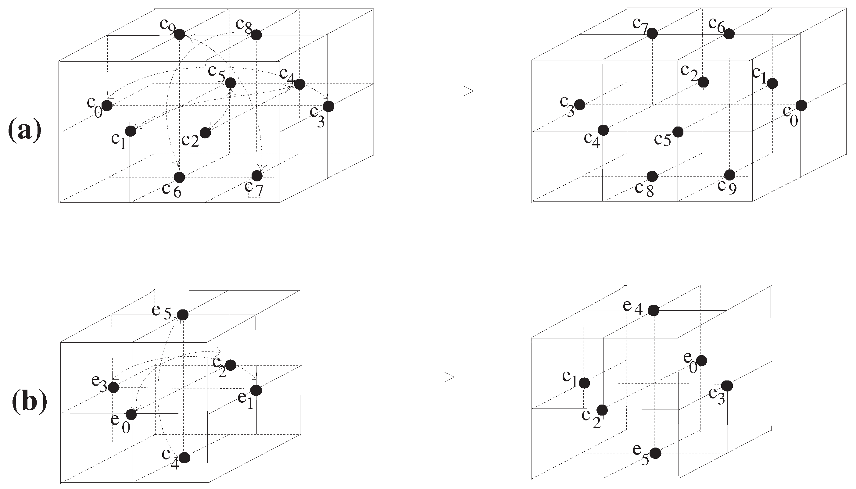
By Proposition 3 and Example 5, it turns out that each of , , and is not trivial. Despite this situation, in this section, we prove that each of , and does not have the FPP (see Theorem 2).
Theorem 2. (1) does not have the AFPP.
(2) does not have the AFPP.
Proof. (1) Let us consider the self-bijection
f of
using the composite of the three different types of reflections
, and
of
, as follows (see
Figure 4a):
is defined as
where the notation “
” in Equation (17) means a mapping from
p to
q and vice versa by using the given maps,
, and
, where
.
Then, we observe that the maps
, and
are special kinds of reflections which are 18-continuous self-bijections of
. Then, we obtain the composite
which is also an 18-continuous self-bijection of
(see
Figure 4a). However, the map
f does not support the
AFPP for
. To be precise, we observe that there is no point
such that
or
is 18-adjacent to
x.
(2) Let us consider the self-bijection
g of
in the following way (see
Figure 4b):
is defined as
Then, we observe that the map g is an 18-continuous bijection on . However, we find that the map g does not support the AFPP for . To be specific, we observe that there is no point such that or is 18-adjacent to x. □
It is obvious that does not have the FPP. However, owing to Proposition 2 and Definition 11, we obtain . Thus, owing to Proposition 3, Theorem 2 and Examples 5 and 6, we have the following:
Corollary 2. For an , the non-triviality of the Euler characteristic of an implies neither the FPP nor the AFPP of the given .
As stated above, in view of the feature of the Euler characteristics of digital
k-surfaces, we can stress that the study of fixed point theory using the current Euler characteristic is quite different from the approach of the typical fixed point theory. Moreover, based on Remarks 5 and 6, we can also point out the following:
Remark 11. (1) The authors of Reference [14] studied a certain Euler characteristic of a digital image using digital homology groups of (see Section 6 of Reference [14]). Moreover, they urged to establish some connection between the Euler characteristic of a k-surface in Reference [5] (or the current version of Definition 11 in the present paper) and their Euler characteristic using the digital homology referred to in Reference [14]. However, it turns out that they are totally different. Thus, in view of Theorem 2 and Corollary 2, their assertions in Reference [14] involving the Euler characteristic of of Reference [5] are too far from the approach of Reference [5] (or the current one). Indeed, we find that their approach in Reference [14] is irrelevant to the current Euler characteristic in Reference [5] (or the current one). (2) In view of Remarks 8 and 9, Definition 11, and Theorem 2, the current Euler characteristic of facilitates the study of digital surfaces of from the viewpoints of digital surface and typical surface theories.
Remark 12. (1) The digital homology in Reference [14] is indeed quite different from the typical homology group in algebraic topology (for more details, see Section 1 of Reference [32]). Furthermore, the digital homology referred to in Reference [14] is also different from the simplicia homology in algebraic topology. Moreover, in view of this situation, the comment in Reference [14] involving his approach to the Euler characteristic of an with the Euler characteristic in Reference [5] (or the current approach) can be incorrect. (2) The digital 6-, 18-, and 26-sphere-like models, , (or , in Figure 1 were firstly introduced in Reference [3,4]. However, the authors used them in Reference [14] with their attribution. 


