Discrete Mutation Hopfield Neural Network in Propositional Satisfiability

 , , and
Abstract
1. Introduction
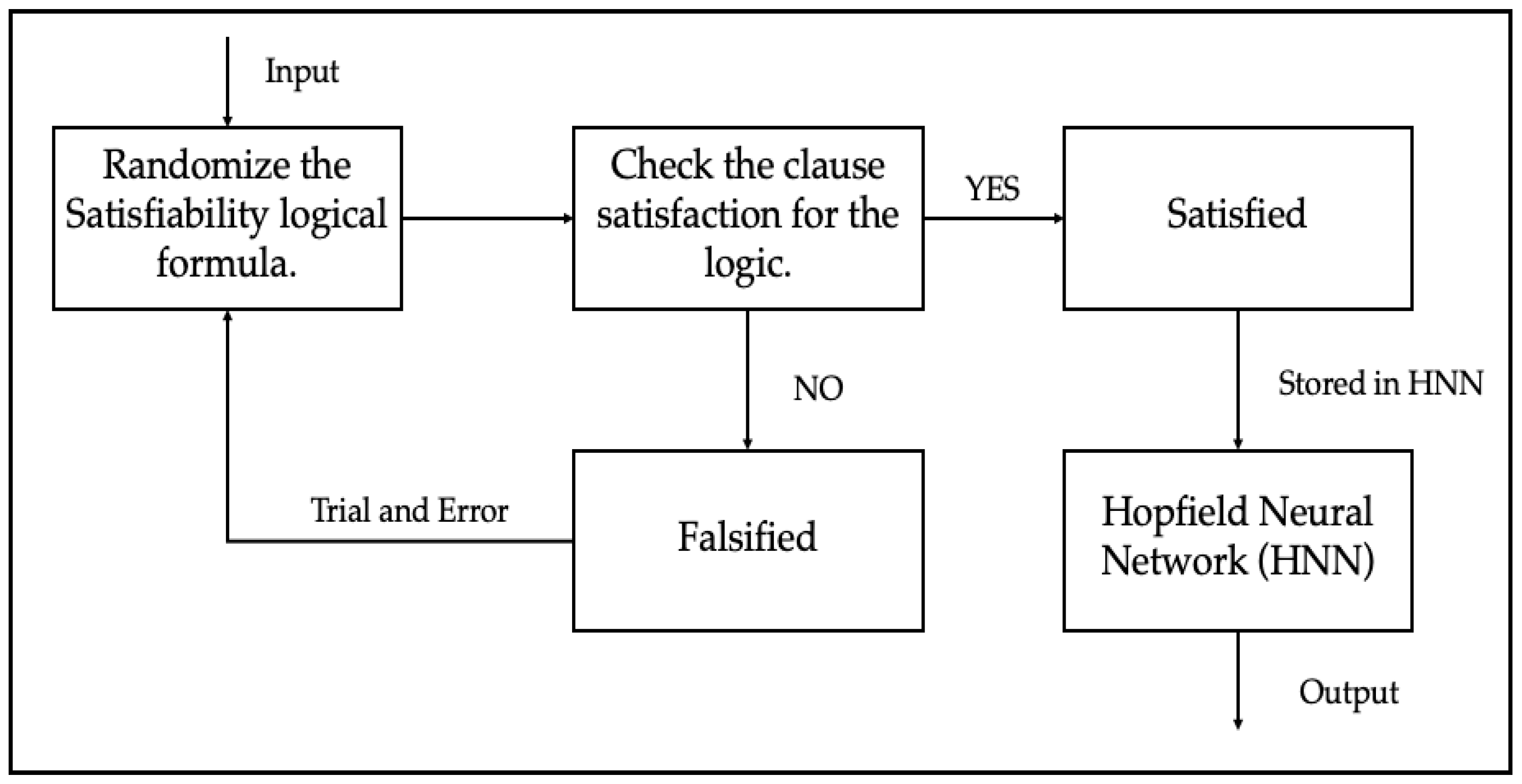
2. Propositional Satisfiability
- Consist of a set of variables, , where . All the variables in the clause will be connected by logical OR .
- A set of literals. A literal is a variable or a negation of variable.
- A set of distinct clauses, . Each clause consists of only literals combined by logical AND .
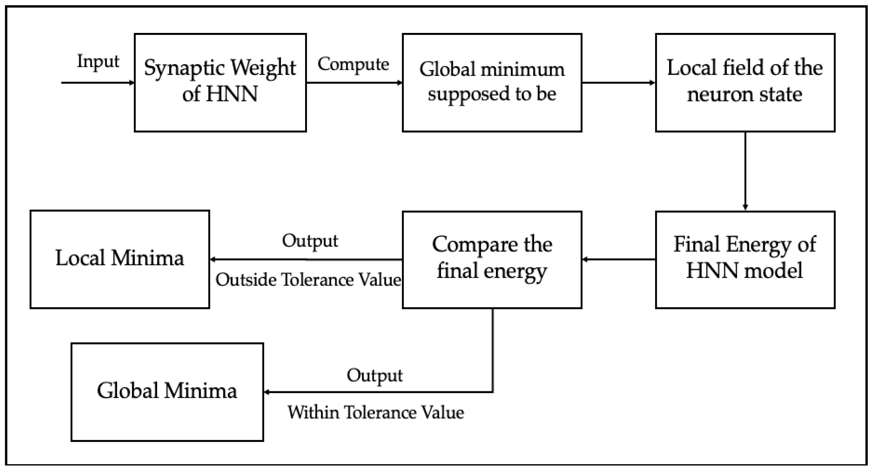
3. Discrete Hopfield Neural Network
4. Mutation Hopfield Neural Network
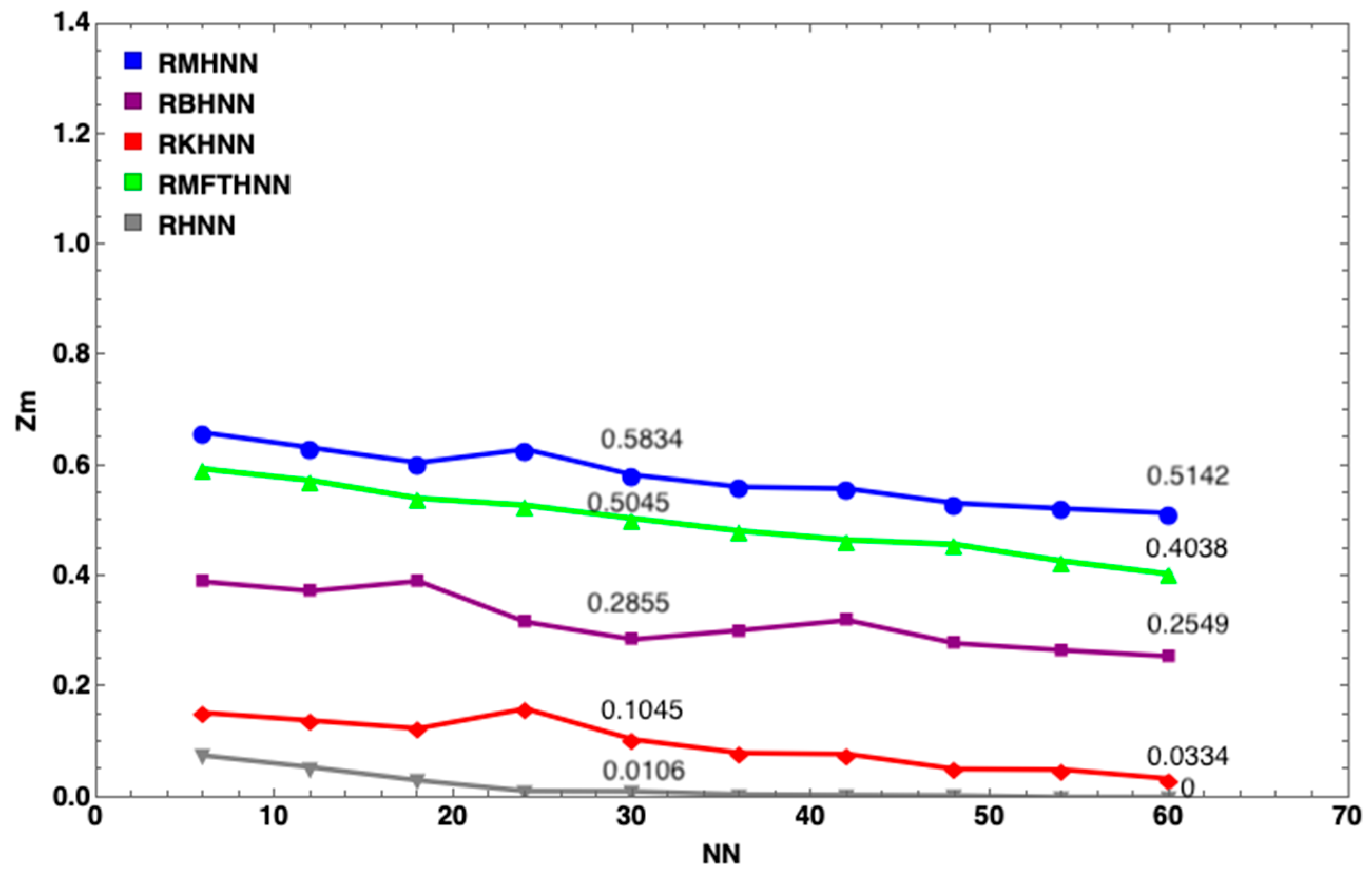
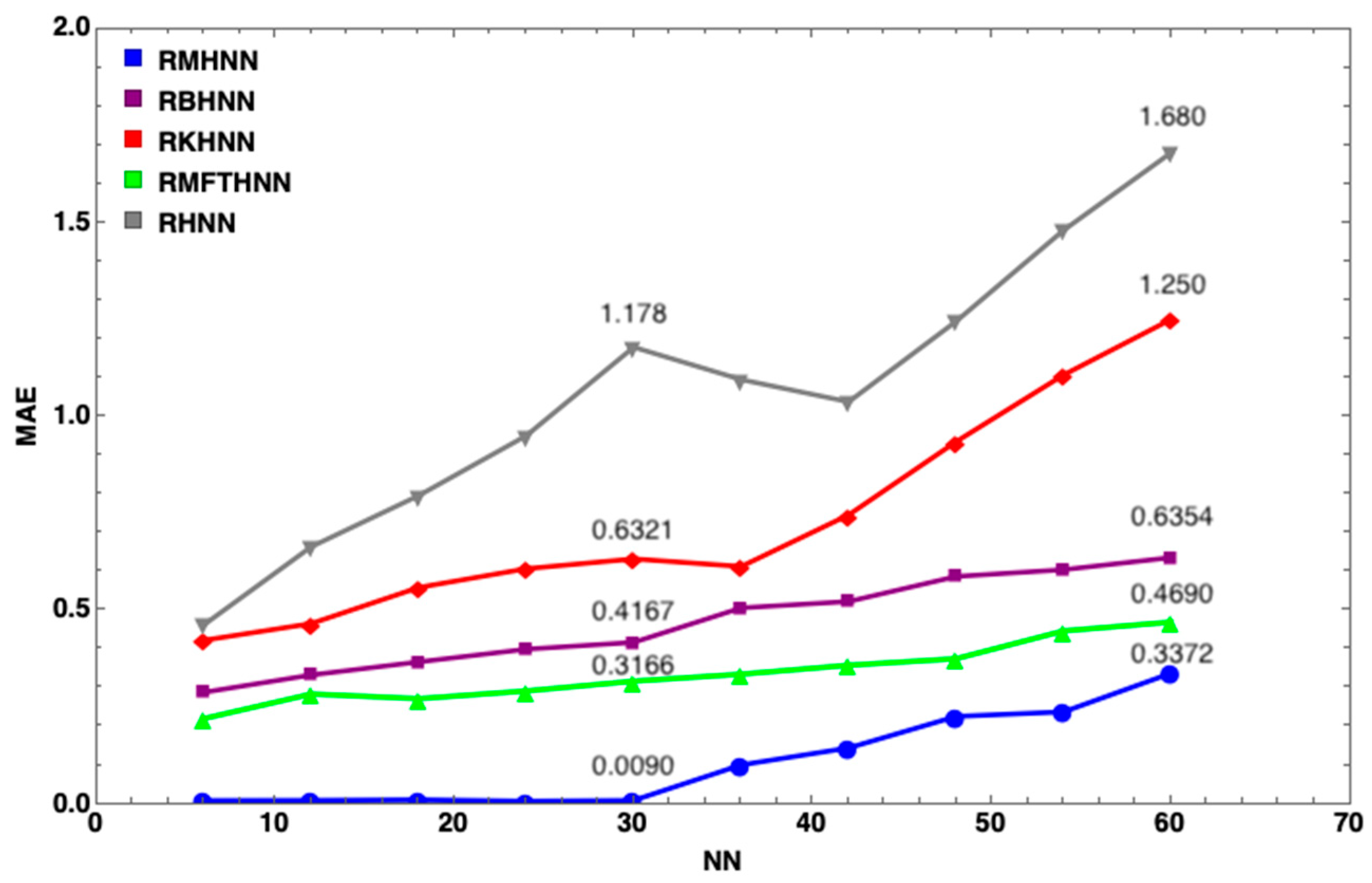
5. HNN Model Performance Evaluation
- is the number of where both elements have the value in ;
- is the number of where is 1 and is −1 in ;
- is the number of where is −1 and is 1 in ;
- is the number of where both elements have the value −1 in .
6. Simulation
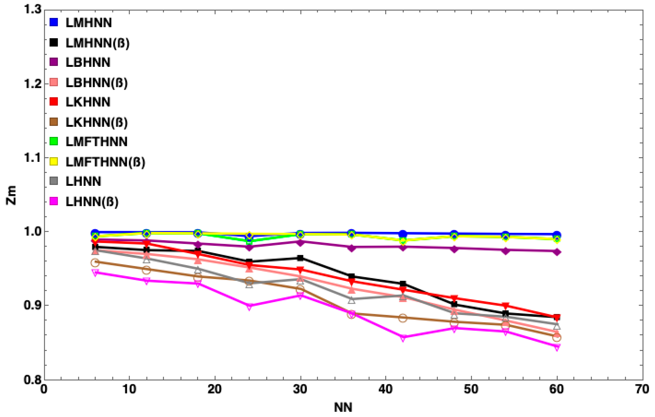
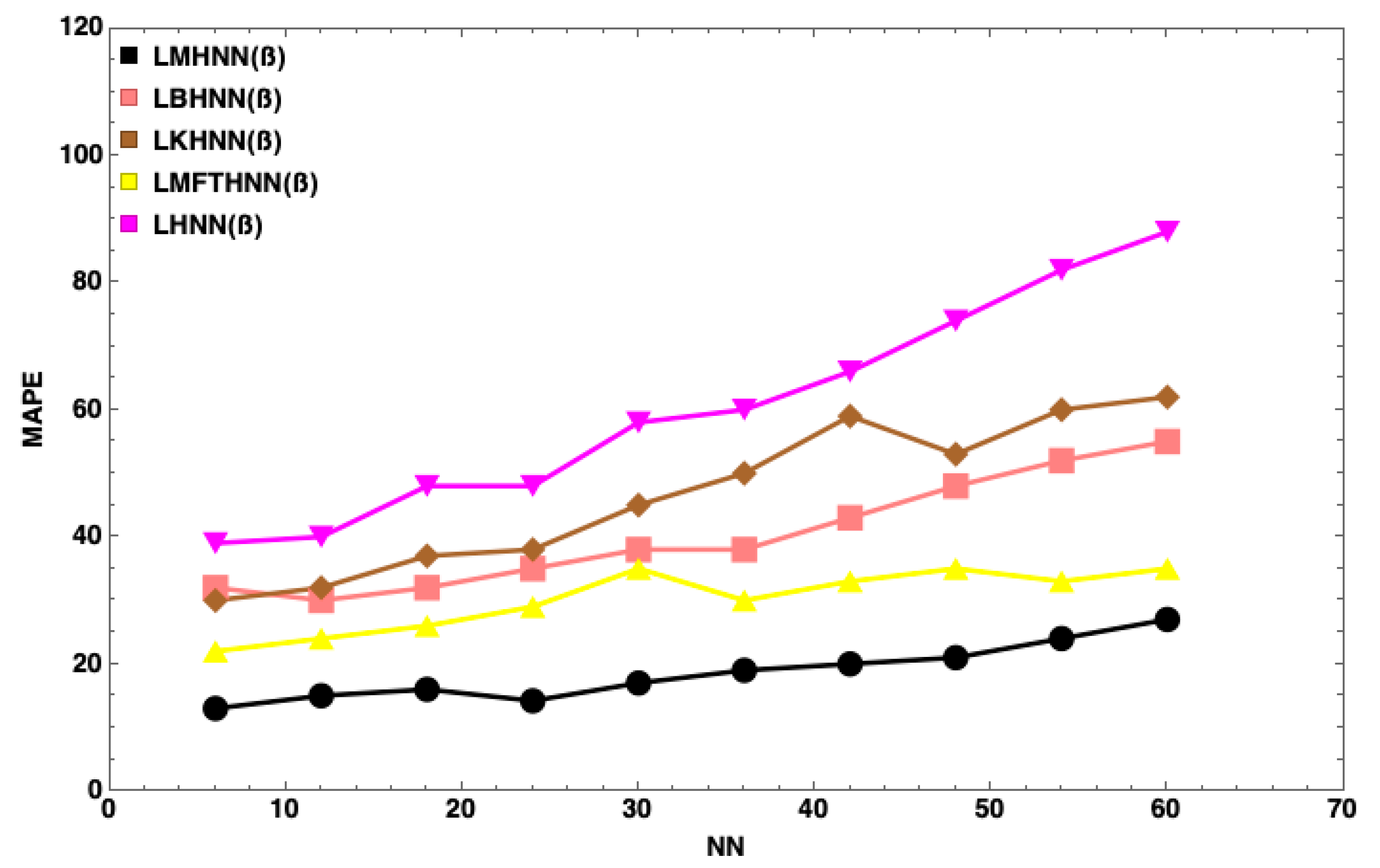
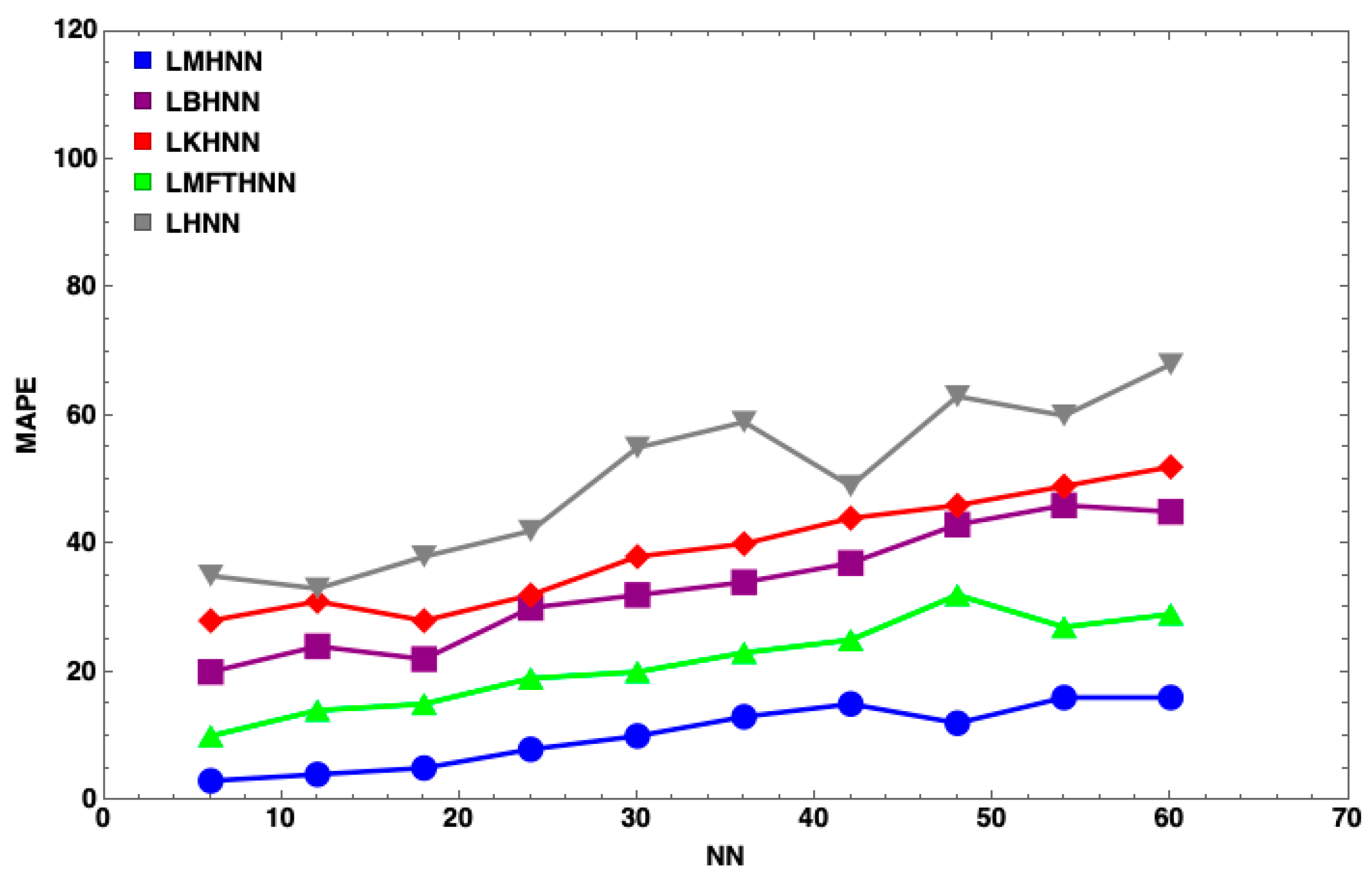
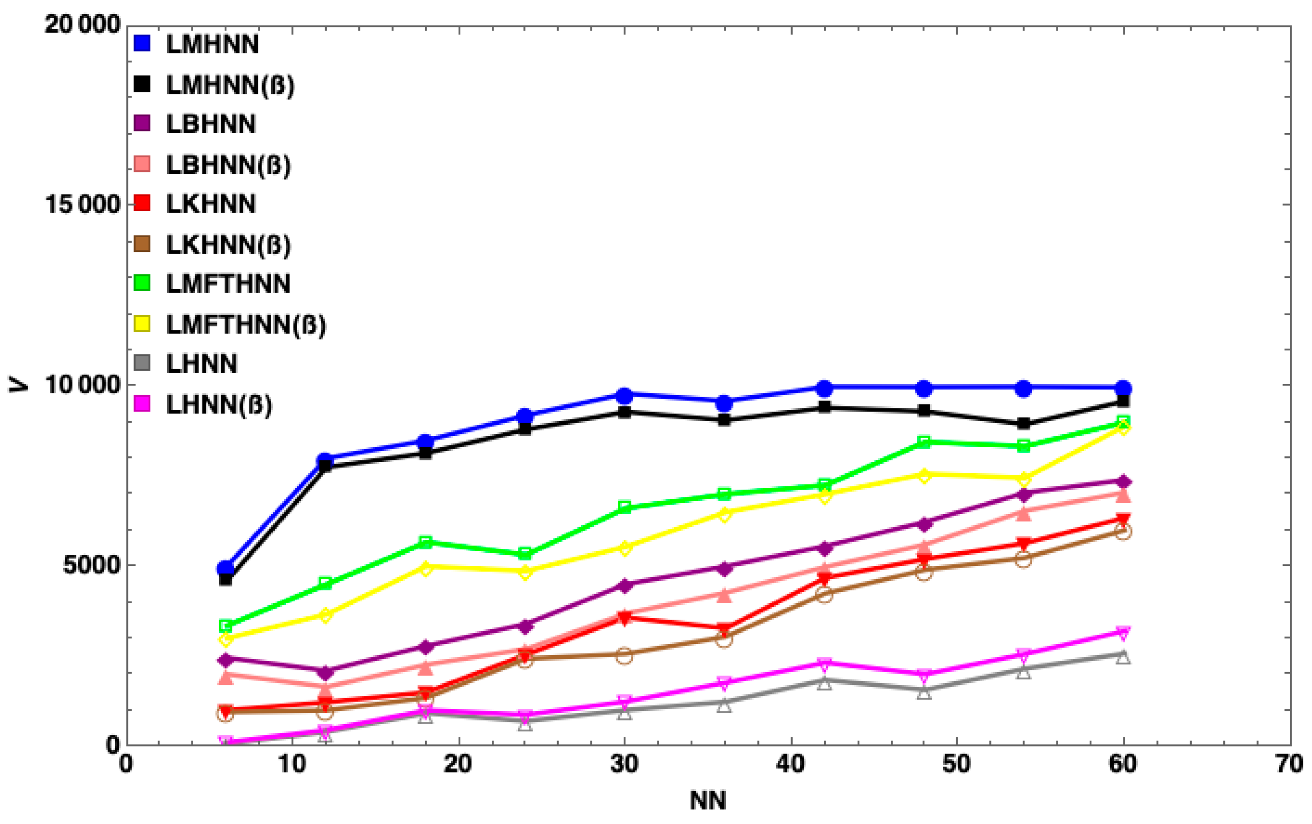
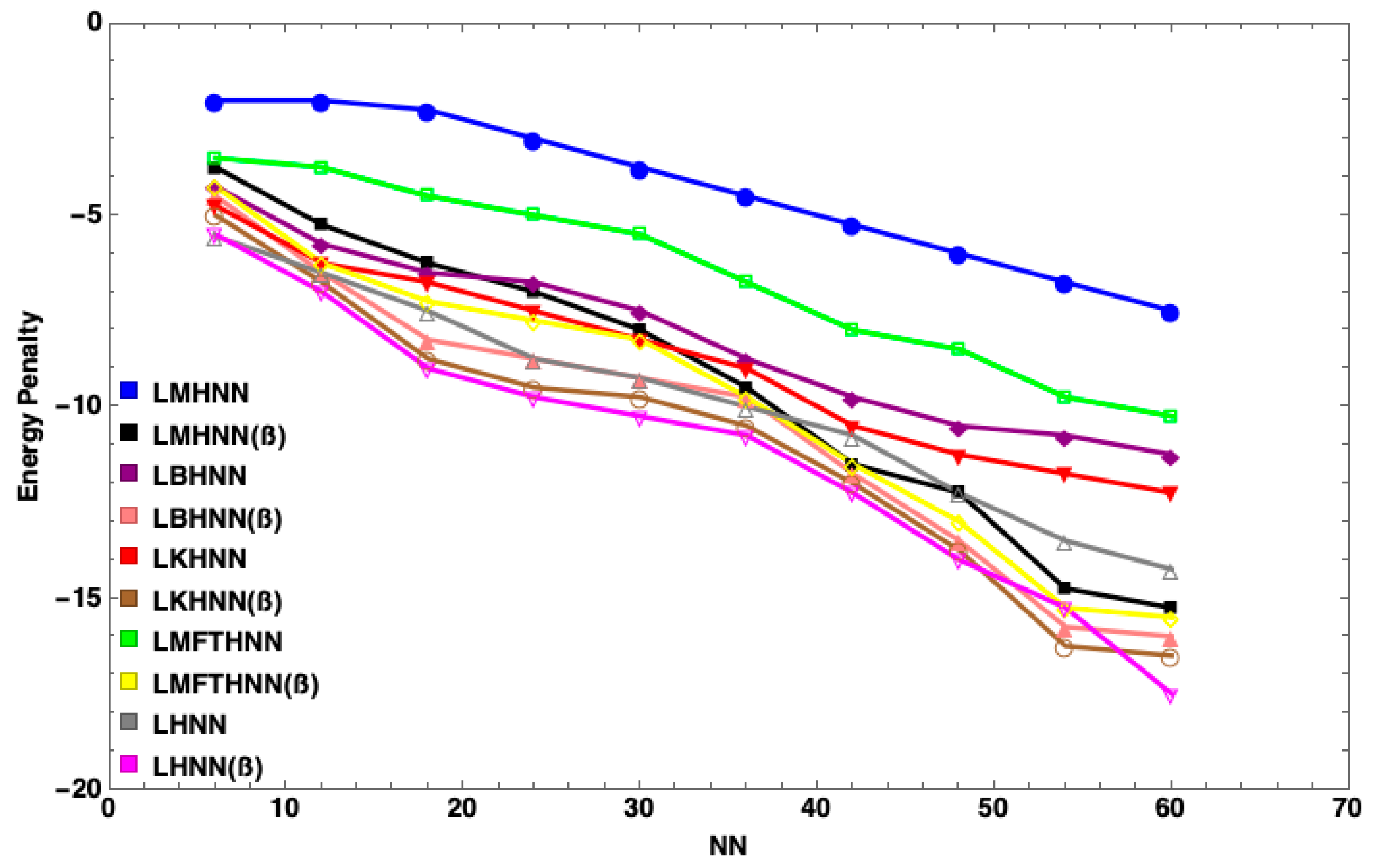
7. Results and Discussion
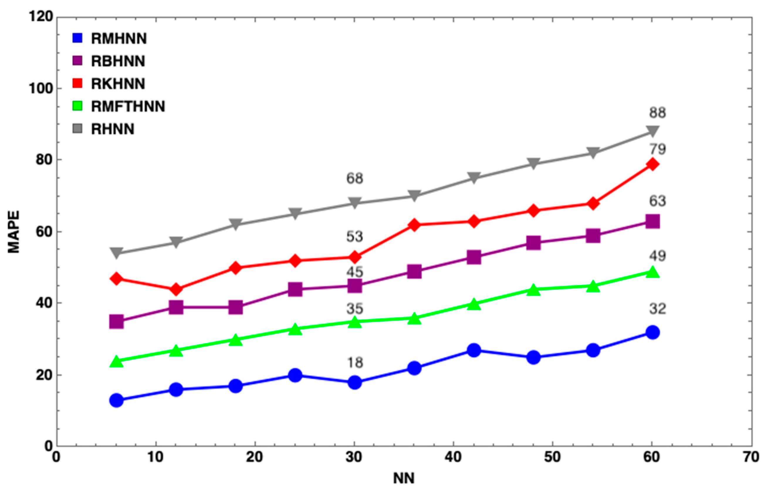
- The MHNN has the lowest energy penalty value compared to other HNN models
- With the same number of neurons, such as , the energy penalty of the HNN has the largest value, followed by the KHNN, BHNN and HNN, indicating that the EDA has the significant effect on the performance of the MHNN.
- has little impact on the MHNN in terms of the energy penalty.
8. Conclusions
Author Contributions
Funding
Conflicts of Interest
Appendix A

References
- Zamanlooy, B.; Mirhassani, M. Mixed-signal VLSI neural network based on continuous valued number system. Neurocomputing 2017, 221, 15–23. [Google Scholar] [CrossRef]
- Fu, Y.; Aldrich, C. Flotation froth image recognition with convolutional neural networks. Miner. Eng. 2019, 132, 183–190. [Google Scholar] [CrossRef]
- Melin, P.; Sanchez, D. Multi-objective optimization for modular granular neural networks applied to pattern recognition. Inf. Sci. 2018, 460, 594–610. [Google Scholar] [CrossRef]
- Turabieh, H.; Mafarja, M.; Li, X. Iterated feature selection algorithms with layered recurrent neural network for software fault prediction. Expert Syst. Appl. 2019, 122, 27–42. [Google Scholar] [CrossRef]
- Grissa, D.; Comte, B.; Petera, M.; Pujos-Guillot, E.; Napoli, A. A hybrid and exploratory approach to knowledge discovery in metabolomic data. Discret. Appl. Math. 2019. [Google Scholar] [CrossRef]
- Hopfield, J.J.; Tank, D.W. “Neural” computation of decisions in optimization problems. Biol. Cybern. 1985, 52, 141–152. [Google Scholar]
- Silva, H.O.; Bastos-Filho, C.J. Inter-domain routing for communication networks using Hierarchical Hopfield neural network. Eng. Appl. Artif. Intell. 2018, 70, 184–198. [Google Scholar] [CrossRef]
- Jayashree, J.; Kumar, S.A. Evolutionary Correlated Gravitational Search Algorithm (ECGS) With Genetic Optimized Hopfield Neural Network (GHNN)—A Hybrid Expert System for Diagnosis of Diabetes. Measurement 2019, 145, 551–558. [Google Scholar] [CrossRef]
- Bafghi, M.S.; Zakeri, A.; Ghasemi, Z. Reductive dissolution of manganese in sulfuric acid in the presence of iron metal. Hydrometallurgy 2008, 90, 207–212. [Google Scholar] [CrossRef]
- Yang, J.; Wang, L.; Wang, Y.; Gou, T. A novel memristive Hopfield neural network with application in associative memory. Neurocomputing 2017, 227, 142–148. [Google Scholar] [CrossRef]
- Peng, M.; Gupta, N.K.; Armitage, A.F. An investigation into the improvement of local minima of the Hopfield Network. Neural Netw. 1996, 90, 207–212. [Google Scholar] [CrossRef]
- Yang, G.; Wu, S.; Jin, Q.; Xu, J. A hybrid approach based on stochastic competitive Hopfield neural network and efficient genetic algorithm for frequency assignment problem. Appl. Soft Comput. 2016, 39, 104–116. [Google Scholar] [CrossRef]
- Zhang, X.; Li, C.; Huang, T. Hybrid Impulsive and switching Hopfield neural networks with state-dependent impulses. Neural Netw. 2017, 93, 176–184. [Google Scholar] [CrossRef] [PubMed]
- Kobayashi, M. Symmetric quaternionic Hopfield neural networks. Neurocomputing 2017, 227, 110–114. [Google Scholar] [CrossRef]
- Larrañaga, P.; Karshenas, H.; Bielza, C.; Santana, R. A review on probabilistic graphical models in evolutionary computation. J. Heuristics 2012, 18, 795–819. [Google Scholar] [CrossRef]
- Gao, S.; De Silva, C.W. Estimation distribution algorithms on constrained optimization problems. Appl. Math. Comput. 2018, 339, 323–345. [Google Scholar] [CrossRef]
- Zhao, F.; Shao, Z.; Wang, J.; Zhang, C. A hybrid differential evolution and estimation of distributed algorithm based on neighbourhood search for job shop scheduling problem. Int. J. Prod. Res. 2016, 54, 1039–1060. [Google Scholar] [CrossRef]
- Gu, W.; Wu, Y.; Zhang, G. A hybrid Univariate Marginal Distribution Algorithm for dynamic economic dispatch of unites considering valve-point effects and ramp rates. Int. Trans. Electr. Energy Syst. 2015, 25, 374–392. [Google Scholar] [CrossRef]
- Fard, M.R.; Mohaymany, A.S. A copula-based estimation of distribution algorithm for calibration of microscopic traffic models. Transp. Res. Part C 2019, 98, 449–470. [Google Scholar] [CrossRef]
- Gobeyn, S.; Mouton, A.M.; Cord, A.F.; Kaim, A.; Volk, M.; Goethals, P.L. Evolutionary algorithms for species distribution modelling: A review in the context of machine learning. Ecol. Model. 2019, 392, 179–195. [Google Scholar] [CrossRef]
- Wang, J. Hopfield neural network based on estimation of distribution for two-page crossing number problem. IEEE Trans. Circuits Syst. II 2008, 55, 797–801. [Google Scholar] [CrossRef]
- Hu, L.; Sun, F.; Xu, H.; Liu, H.; Zhang, X. Mutation Hopfield neural network and its applications. Inf. Sci. 2011, 181, 92–105. [Google Scholar] [CrossRef]
- Glaßer, C.; Jonsson, P.; Martin, B. Circuit satisfiability and constraint satisfaction around Skolem Arithmetic. Theor. Comput. Sci. 2017, 703, 18–36. [Google Scholar] [CrossRef]
- Budinich, M. The Boolean Satisfiability Problem in Clifford algebra. Theor. Comput. Sci. 2019. [Google Scholar] [CrossRef]
- Jensen, L.S.; Kaufmann, I.; Larsen, K.G.; Nielsen, S.M.; Srba, J. Model checking and synthesis for branching multi-weighted logics. J. Log. Algebraic Methods Program. 2019, 105, 28–46. [Google Scholar] [CrossRef]
- Małysiak-Mrozek, B. Uncertainty, imprecision, and many-valued logics in protein bioinformatics. Math. Biosci. 2019, 309, 143–162. [Google Scholar] [CrossRef] [PubMed]
- Christoff, Z.; Hansen, J.U. A logic for diffusion in social networks. J. Appl. Log. 2015, 13, 48–77. [Google Scholar] [CrossRef]
- Xue, C.; Xiao, S.; Ouyang, C.H.; Li, C.C.; Gao, Z.H.; Shen, Z.F.; Wu, Z.S. Inverted mirror image molecular beacon-based three concatenated logic gates to detect p53 tumor suppressor gene. Anal. Chim. Acta 2019, 1051, 179–186. [Google Scholar] [CrossRef]
- Kasihmuddin, M.S.M.; Mansor, M.A.; Sathasivam, S. Discrete Hopfield Neural Network in Restricted Maximum k-Satisfiability Logic Programming. Sains Malays. 2018, 47, 1327–1335. [Google Scholar] [CrossRef]
- Tasca, L.C.; de Freitas, E.P.; Wagner, F.R. Enhanced architecture for programmable logic controllers targeting performance improvements. Microprocess. Microsyst. 2018, 61, 306–315. [Google Scholar] [CrossRef]
- Wan Abdullah, W.A.T. Logic programming on a neural network. Int. J. Intell. Syst. 1992, 7, 513–519. [Google Scholar] [CrossRef]
- Sathasivam, S. First Order Logic in Neuro-Symbolic Integration. Far East J. Math. Sci. 2012, 61, 213–229. [Google Scholar]
- Mansor, M.A.; Sathasivam, S. Accelerating Activation Function for 3-Satisfiability Logic Programming. Int. J. Intell. Syst. Appl. 2016, 8, 44–50. [Google Scholar]
- Sathasivam, S. Upgrading logic programming in Hopfield network. Sains Malays. 2010, 39, 115–118. [Google Scholar]
- Sathasivam, S. Learning Rules Comparison in Neuro-Symbolic Integration. Int. J. Appl. Phys. Math. 2011, 1, 129–132. [Google Scholar] [CrossRef]
- Mansor, M.A.; Sathasivam, S. Performance analysis of activation function in higher order logic programming. AIP Conf. Proc. 2016, 1750. [Google Scholar]
- Kasihmuddin, M.S.B.M.; Sathasivam, S. Accelerating activation function in higher order logic programming. AIP Conf. Proc. 2016, 1750. [Google Scholar]
- Yoon, H.U.; Lee, D.W. Subplanner Algorithm to Escape from Local Minima for Artificial Potential Function Based Robotic Path Planning. Int. J. Fuzzy Log. Intell. Syst. 2018, 18, 263–275. [Google Scholar] [CrossRef]
- Velavan, M.; Yahya, Z.R.; Abdul Halif, M.N.; Sathasivam, S. Mean field theory in doing logic programming using hopfield network. Mod. Appl. Sci. 2016, 10, 154. [Google Scholar] [CrossRef]
- Alzaeemi, S.A.; Sathasivam, S. Linear kernel Hopfield neural network approach in horn clause programming. AIP Conf. Proc. 2018, 1974, 020107. [Google Scholar]
- Paul, A.; Poloczek, M.; Williamson, D.P. Simple Approximation Algorithms for Balanced MAX 2SAT. Algorithmica 2018, 80, 995–1012. [Google Scholar] [CrossRef]
- Morais, C.V.; Zimmer, F.M.; Magalhaes, S.G. Inverse freezing in the Hopfield fermionic Ising spin glass with a transverse magnetic field. Phys. Lett. A 2011, 375, 689–697. [Google Scholar] [CrossRef][Green Version]
- Barra, A.; Beccaria, M.; Fachechi, A. A new mechanical approach to handle generalized Hopfield neural networks. Neural Netw. 2018, 106, 205–222. [Google Scholar] [CrossRef] [PubMed]
- Zarco, M.; Froese, T. Self-modeling in Hopfield neural networks with continuous activation function. Procedia Comput. Sci. 2018, 123, 573–578. [Google Scholar] [CrossRef]
- Abdullah, W.A.T.W. The logic of neural networks. Phys. Lett. A 1993, 176, 202–206. [Google Scholar] [CrossRef]
- Kumar, S.; Singh, M.P. Pattern recall analysis of the Hopfield neural network with a genetic algorithm. Comput. Math. Appl. 2010, 60, 1049–1057. [Google Scholar] [CrossRef][Green Version]
- Salcedo-Sanz, S.; Ortiz-García, E.G.; Pérez-Bellido, Á.M.; Portilla-Figueras, A.; López-Ferreras, F. On the performance of the LP-guided Hopfield network-genetic algorithm. Comput. Oper. Res. 2009, 36, 2210–2216. [Google Scholar] [CrossRef]
- Wu, J.; Long, J.; Liu, M. Evolving RBF neural networks for rainfall prediction using hybrid particle swarm optimization and genetic algorithm. Neurocomputing 2015, 148, 136–142. [Google Scholar] [CrossRef]
- Chen, D.; Chen, Q.; Leon, A.S.; Li, R. A genetic algorithm parallel strategy for optimizing the operation of reservoir with multiple eco-environmental objectives. Water Resour. Manag. 2016, 30, 2127–2142. [Google Scholar] [CrossRef]
- García-Martínez, C.; Rodriguez, F.J.; Lozano, M. Genetic Algorithms. Handb. Heuristics 2018, 431–464. [Google Scholar] [CrossRef]
- Tian, J.; Hao, X.; Gen, M. A hybrid multi-objective EDA for robust resource constraint project scheduling with uncertainty. Comput. Ind. Eng. 2019, 130, 317–326. [Google Scholar] [CrossRef]
- Fang, H.; Zhou, A.; Zhang, H. Information fusion in offspring generation: A case study in DE and EDA. Swarm Evol. Comput. 2018, 42, 99–108. [Google Scholar] [CrossRef]
- Kasihmuddin, M.S.M.; Mansor, M.A.; Sathasivam, S. Hybrid Genetic Algorithm in the Hopfield Network for Logic Satisfiability Problem. Pertanika J. Sci. Technol. 2017, 1870, 050001. [Google Scholar]
- Bag, S.; Kumar, S.K.; Tiwari, M.K. An efficient recommendation generation using relevant Jaccard similarity. Inf. Sci. 2019, 483, 53–64. [Google Scholar] [CrossRef]
- Pachayappan, M.; Panneerselvam, R. A Comparative Investigation of Similarity Coefficients Applied to the Cell Formation Problem using Hybrid Clustering Algorithms. Mater. Today: Proc. 2018, 5, 12285–12302. [Google Scholar] [CrossRef]
- Cardenas, C.E.; McCarroll, R.E.; Court, L.E.; Elgohari, B.A.; Elhalawani, H.; Fuller, C.D.; Kamal, M.J.; Meheissen, M.A.; Mohamed, A.S.; Rao, A.; et al. Deep learning algorithm for auto-delineation of high-risk oropharyngeal clinical target volumes with built-in dice similarity coefficient parameter optimization function. Int. J. Radiat. Oncol. Biol. Phys. 2018, 101, 468–478. [Google Scholar] [CrossRef]
- Ikemoto, S.; DallaLibera, F.; Hosoda, K. Noise-modulated neural networks as an application of stochastic resonance. Neurocomputing 2018, 277, 29–37. [Google Scholar] [CrossRef]
- Ong, P.; Zainuddin, Z. Optimizing wavelet neural networks using modified cuckoo search for multi-step ahead chaotic time series prediction. Appl. Soft Comput. 2019, 80, 374–386. [Google Scholar] [CrossRef]
- Kasihmuddin, M.S.M.; Mansor, M.A.; Sathasivam, S. Maximum 2 satisfiability logical rule in restrictive learning environment. AIP Publ. 2018, 1974, 020021. [Google Scholar]
- McCulloch, W.S.; Pitts, W. A logical calculus of the ideas immanent in nervous activity. Bull. Math. Biophys. 1943, 5, 115–133. [Google Scholar] [CrossRef]
- Cheng, S.; Chen, J.; Wang, L. Information perspective to probabilistic modeling: Boltzmann machines versus born machines. Entropy 2018, 20, 583. [Google Scholar] [CrossRef]
- Mansor, M.A.; Kasihmuddin, M.S.M.; Sathasivam, S. Modified Artificial Immune System Algorithm with Elliot Hopfield Neural Network for 3-Satisfiability Programming. J. Inform. Math. Sci. 2019, 11, 81–98. [Google Scholar]
- Li, K.; Lu, W.; Liang, C.; Wang, B. Intelligence in Tourism Management: A Hybrid FOA-BP Method on Daily Tourism Demand Forecasting with Web Search Data. Mathematics 2019, 7, 531. [Google Scholar] [CrossRef]
- Frosini, A.; Vuillon, L. Tomographic reconstruction of 2-convex polyominoes using dual Horn clauses. Theor. Comput. Sci. 2019, 777, 329–337. [Google Scholar] [CrossRef]
- Shu, J.; Xiong, L.; Wu, T.; Liu, Z. Stability Analysis of Quaternion-Valued Neutral-Type Neural Networks with Time-Varying Delay. Mathematics 2019, 7, 101. [Google Scholar] [CrossRef]
- Yun, B.I. A Neural Network Approximation Based on a Parametric Sigmoidal Function. Mathematics 2019, 7, 262. [Google Scholar] [CrossRef]
- Wu, Z.; Christofides, P.D. Economic Machine-Learning-Based Predictive Control of Nonlinear Systems. Mathematics 2019, 7, 494. [Google Scholar] [CrossRef]
- Kanokoda, T.; Kushitani, Y.; Shimada, M.; Shirakashi, J.I. Gesture Prediction using Wearable Sensing Systems with Neural Networks for Temporal Data Analysis. Sensors 2019, 19, 710. [Google Scholar] [CrossRef]
- Wong, W.; Chee, E.; Li, J.; Wang, X. Recurrent Neural Network-Based Model Predictive Control for Continuous Pharmaceutical Manufacturing. Mathematics 2018, 6, 242. [Google Scholar] [CrossRef]
- Shah, F.; Debnath, L. Wavelet Neural Network Model for Yield Spread Forecasting. Mathematics 2017, 5, 72. [Google Scholar] [CrossRef]


| No | Similarity Coefficient | Similarity Representation |
|---|---|---|
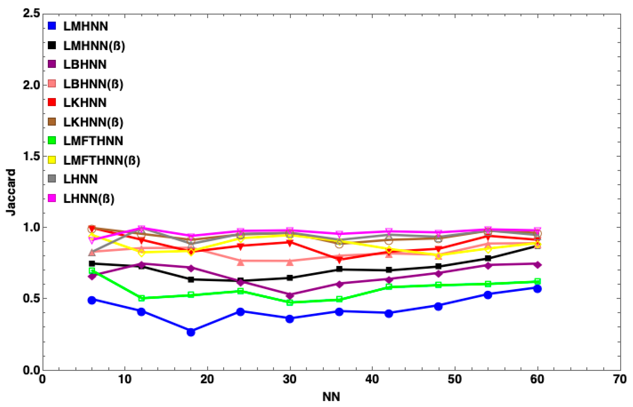
| 1 | Jaccard’s Index [54] | |
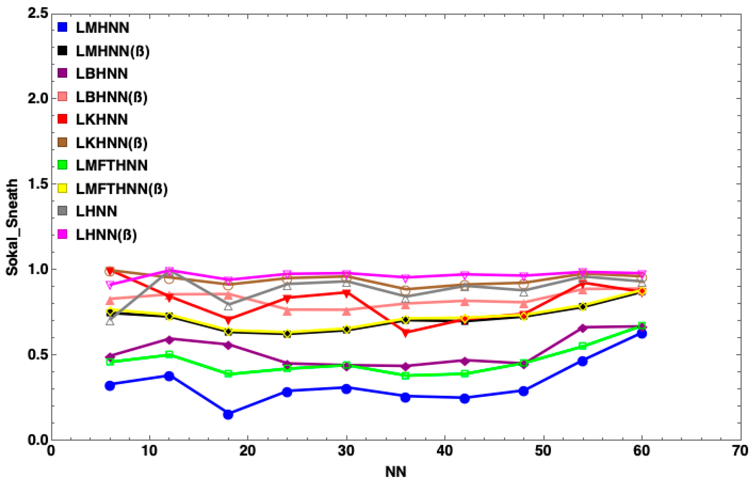
| 2 | Sokal Sneath 2 [55] | |
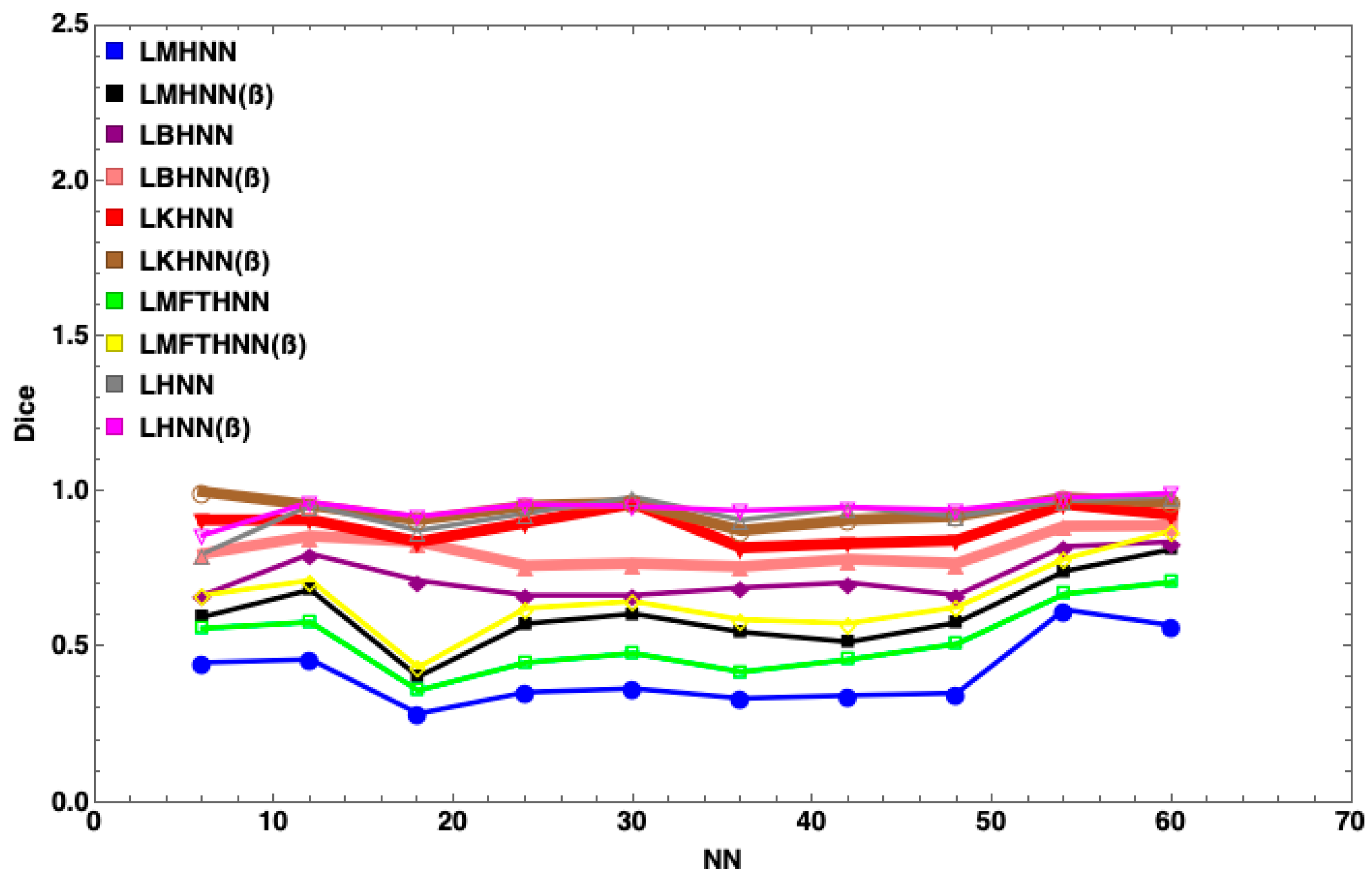
| 3 | Dice [56] |
| Parameter | Parameter Value |
|---|---|
| Neuron Combination | 100 |
| Tolerance Value (∂) | 0.001 |
| Number of Learning (Ω) | 100 |
| No_Neuron String | 100 |
| Selection_Rate | 0.1 |
| Mutation Rate | 0.01 |
| Parameter | Parameter Value |
|---|---|
| Neuron Combination | 100 |
| Tolerance Value (∂) | 0.001 |
| Number of Learning (Ω) | 100 |
| No_Neuron String | 100 |
| Selection_Rate | 0.1 |
| Parameter | Parameter Value |
|---|---|
| Neuron Combination | 100 |
| Tolerance Value (∂) | 0.001 |
| Number of Learning (Ω) | 100 |
| No_Neuron String | 100 |
| Selection_Rate | 0.1 |
| Type of Kernel | Linear Kernel |
| Parameter | Parameter Value |
|---|---|
| Neuron Combination | 100 |
| Tolerance Value (∂) | 0.001 |
| Number of Learning (Ω) | 100 |
| No_Neuron String | 100 |
| Selection_Rate | 0.1 |
| Temperature (T) | 70 |
| Parameter | Parameter Value |
|---|---|
| Neuron Combination | 100 |
| Tolerance Value (∂) | 0.001 |
| Number of Learning (Ω) | 100 |
| No_Neuron String | 100 |
| Selection_Rate | 0.1 |
| Temperature (T) | 70 |
| Activation Function | Hyperbolic Tangent (HTAF) |
© 2019 by the authors. Licensee MDPI, Basel, Switzerland. This article is an open access article distributed under the terms and conditions of the Creative Commons Attribution (CC BY) license (http://creativecommons.org/licenses/by/4.0/).
Share and Cite
Mohd Kasihmuddin, M.S.; Mansor, M.A.; Md Basir, M.F.; Sathasivam, S. Discrete Mutation Hopfield Neural Network in Propositional Satisfiability. Mathematics 2019, 7, 1133. https://doi.org/10.3390/math7111133
Mohd Kasihmuddin MS, Mansor MA, Md Basir MF, Sathasivam S. Discrete Mutation Hopfield Neural Network in Propositional Satisfiability. Mathematics. 2019; 7(11):1133. https://doi.org/10.3390/math7111133
Chicago/Turabian StyleMohd Kasihmuddin, Mohd Shareduwan, Mohd. Asyraf Mansor, Md Faisal Md Basir, and Saratha Sathasivam. 2019. "Discrete Mutation Hopfield Neural Network in Propositional Satisfiability" Mathematics 7, no. 11: 1133. https://doi.org/10.3390/math7111133
APA StyleMohd Kasihmuddin, M. S., Mansor, M. A., Md Basir, M. F., & Sathasivam, S. (2019). Discrete Mutation Hopfield Neural Network in Propositional Satisfiability. Mathematics, 7(11), 1133. https://doi.org/10.3390/math7111133