Impact of Parameter Variability and Environmental Noise on the Klausmeier Model of Vegetation Pattern Formation

Abstract
:1. Introduction
2. Model and Methods
2.1. Model Description
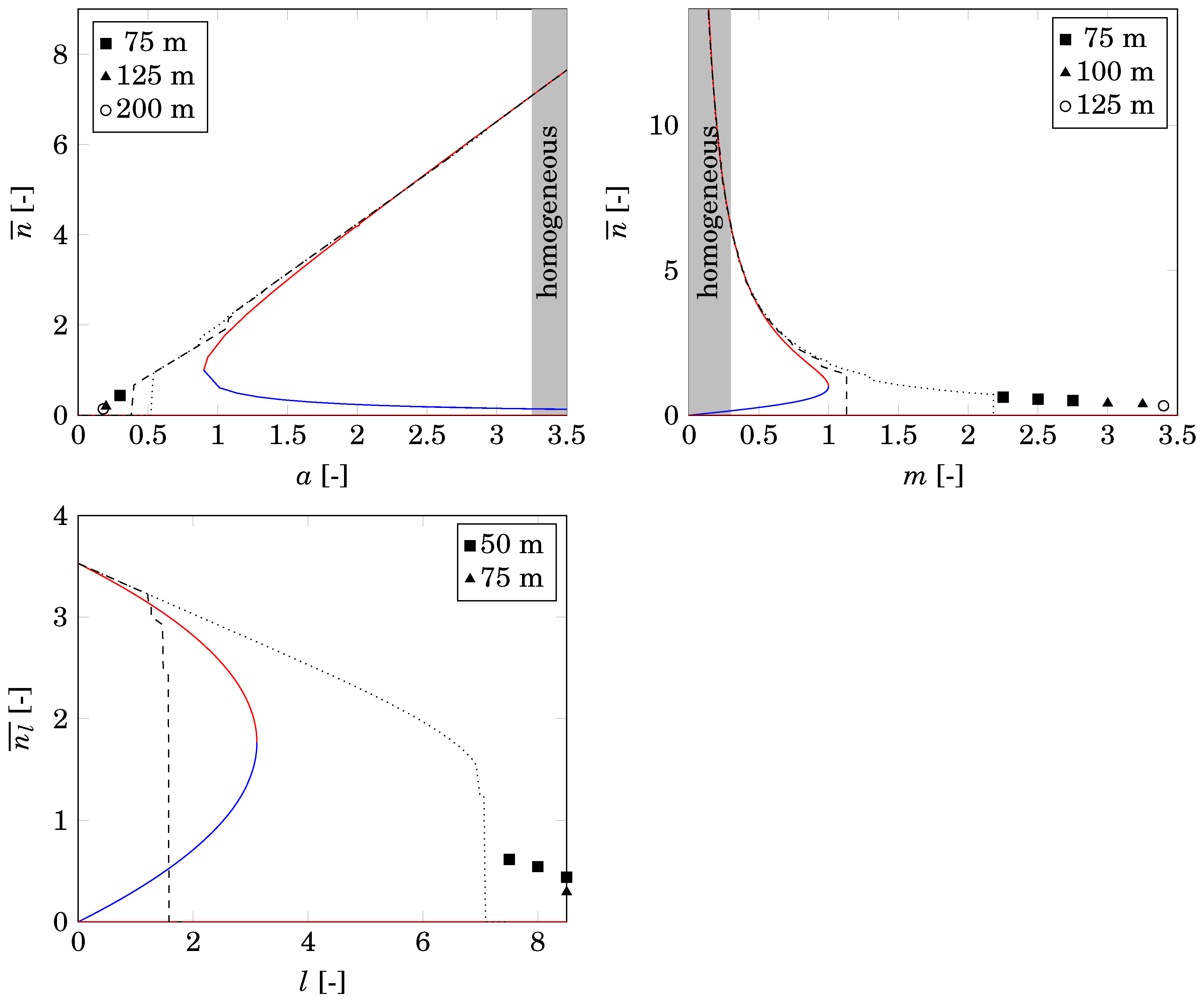
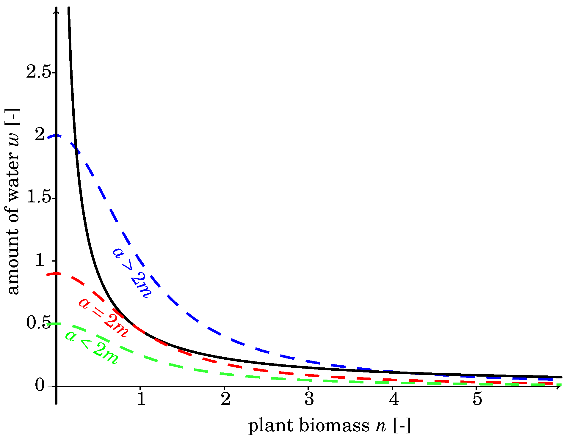
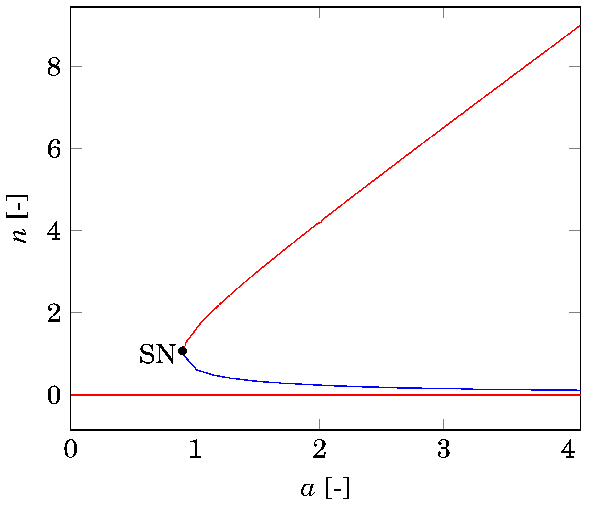
2.2. Nonspatial Equilibria
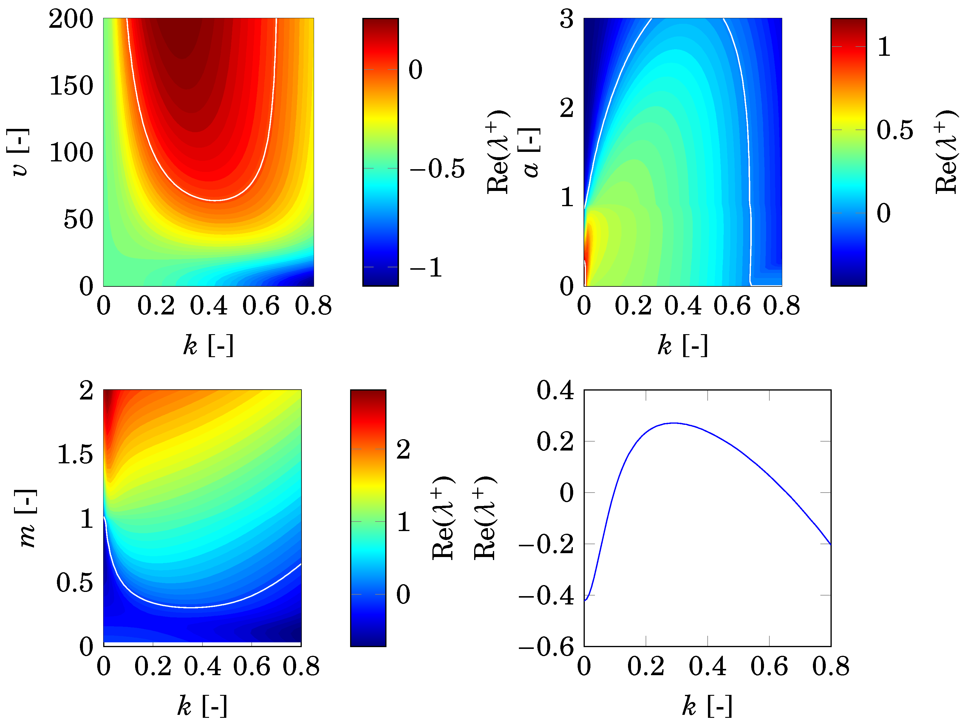
2.3. Differential Flow-Induced Instability
2.4. Considered Parameters
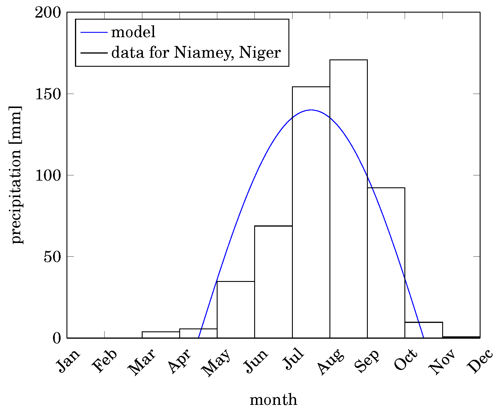
2.5. Precipitation Model
2.6. Stochasticity
2.7. Numerical Treatment
3. Numerical Results
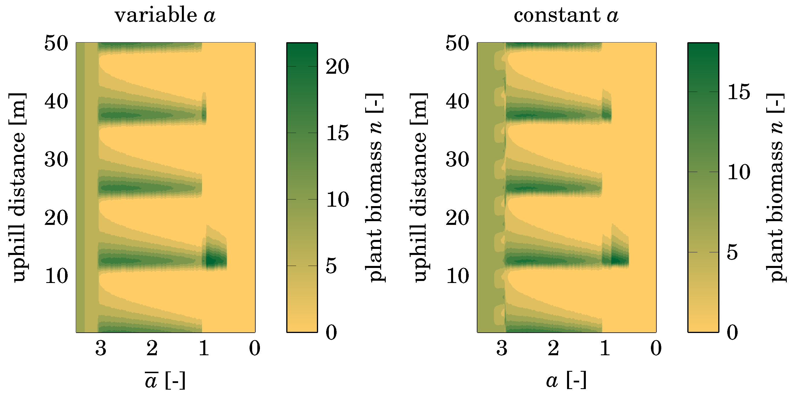
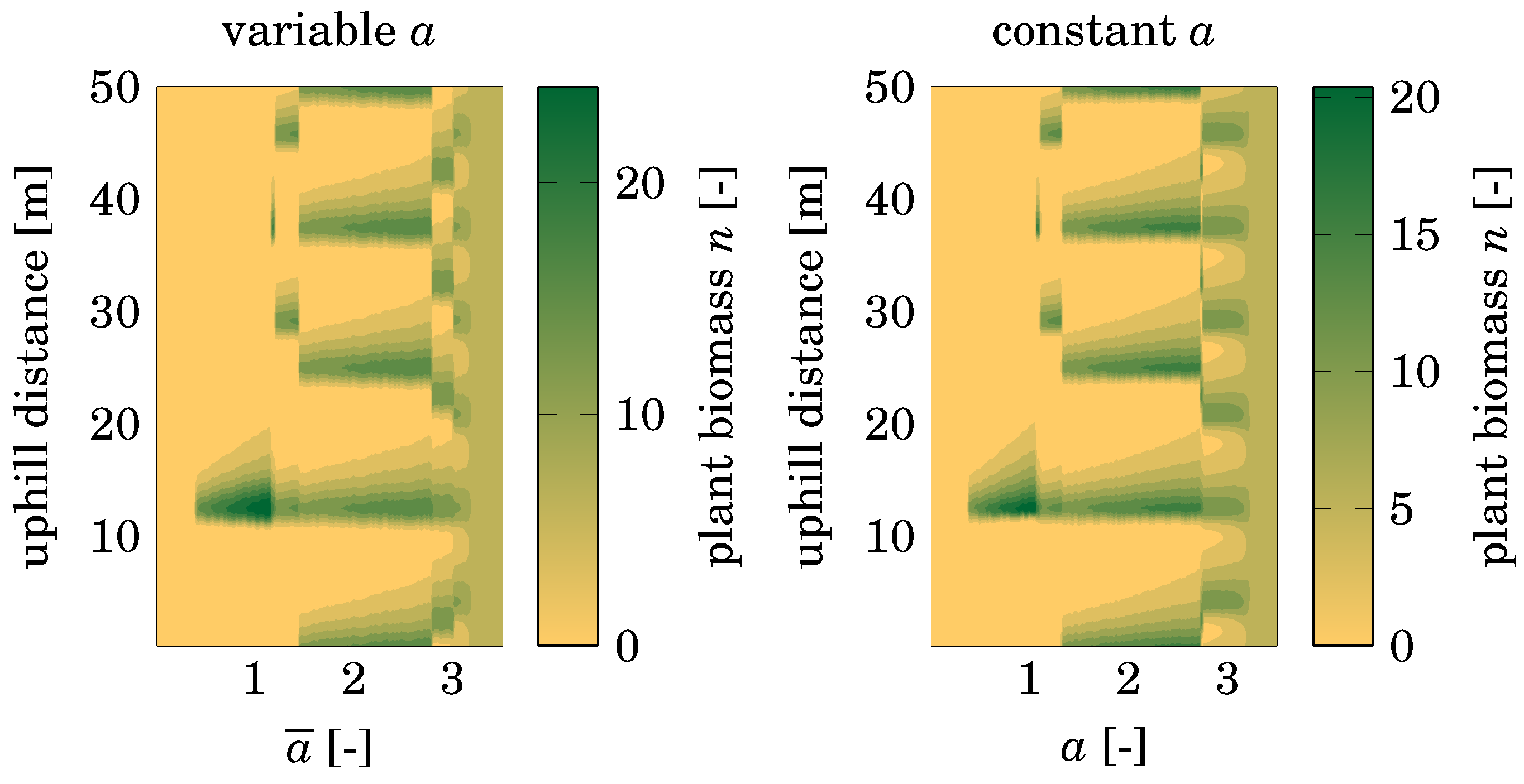
3.1. Precipitation
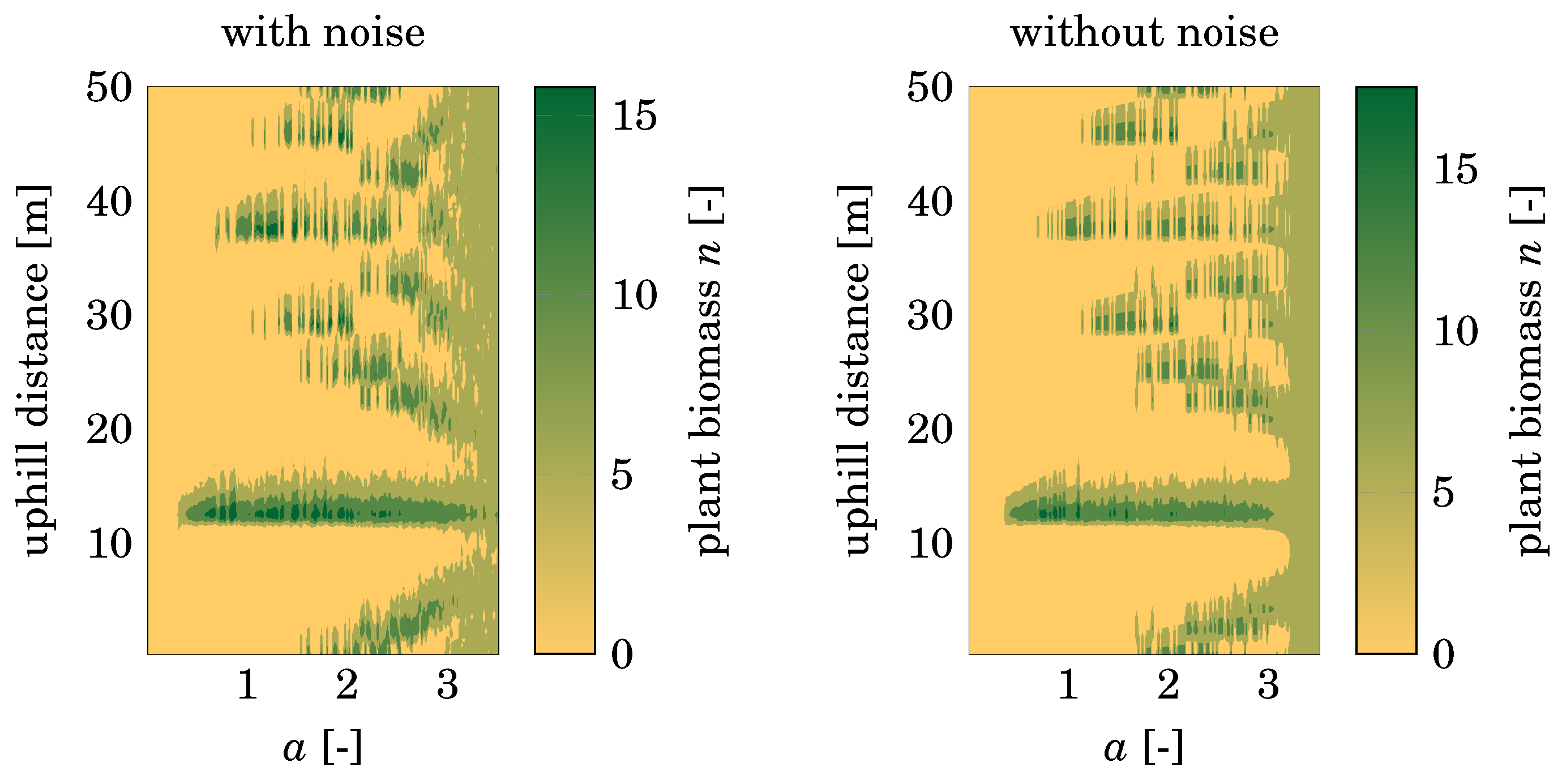
3.2. Stochasticity
3.3. Effect of Pattern Formation
4. Discussion
4.1. Influence of Variable Precipitation
4.2. Dependence on Initial Conditions
4.3. Comparison with Nonspatial Equilibria
5. Conclusions
Acknowledgments
Author Contributions
Conflicts of Interest
Appendix A. Nondimensionalization
Appendix A.1. Nondimensionalization in Terms of Precipitation and Mortality

Appendix A.2. Nondimensionalization in Terms of Evaporation
Appendix B. Default Values

| Physical Parameter | Value | Unit |
|---|---|---|
| T | a | |
| W | kg m | |
| N | kg m | |
| X | m | |
| Y | m | |
| A | 533 | kg m a |
| L | 4 | a |
| R | 100 | m kg a |
| J | 0.003 | — |
| V | 365 | m a |
| M | 1.8 | a |
| D | 1 | m a |
Appendix C. Precipitation Model

References
- Borgogno, F.; D’Odorico, P.; Laio, F.; Ridolfi, L. Mathematical models of vegetation pattern formation in ecohydrology. Rev. Geophys. 2009, 47, RG1005. [Google Scholar] [CrossRef]
- Gillett, J. The plant formations of western British Somaliland and the Harar province of Abyssinia. Misc. Bull. Inf. 1941, 1941, 35–75. [Google Scholar] [CrossRef]
- Macfadyen, W.A. Vegetation patterns in the semi-desert plains of British Somaliland. Geogr. J. 1950, 116, 199–211. [Google Scholar] [CrossRef]
- Deblauwe, V.; Barbier, N.; Couteron, P.; Lejeune, O.; Bogaert, J. The global biogeography of semi-arid periodic vegetation patterns. Glob. Ecol. Biogeogr. 2008, 17, 715–723. [Google Scholar] [CrossRef]
- Meron, E. Nonlinear Physics of Ecosystems, 1st ed.; CRC Press: Boca Raton, FL, USA, 2015. [Google Scholar]
- Gibbens, R.; McNeely, R.; Havstad, K.; Beck, R.; Nolen, B. Vegetation changes in the Jornada Basin from 1858 to 1998. J. Arid Environ. 2005, 61, 651–668. [Google Scholar] [CrossRef]
- Tongway, D.J.; Valentin, C.; Seghieri, J. (Eds.) Banded Vegetation Patterning in Arid and Semiarid Environments; Springer: New York, NY, USA, 2001. [Google Scholar]
- Juergens, N. The biological underpinnings of Namib desert fairy circles. Science 2013, 339, 1618–1621. [Google Scholar] [CrossRef] [PubMed]
- Bromley, J.; Brouwer, J.; Barker, A.; Gaze, S.; Valentine, C. The role of surface water redistribution in an area of patterned vegetation in a semi-arid environment, south-west Niger. J. Hydrol. 1997, 198, 1–29. [Google Scholar] [CrossRef]
- White, L.P. Vegetation stripes on sheet wash surfaces. J. Ecol. 1971, 59, 615–622. [Google Scholar] [CrossRef]
- Barbier, N.; Couteron, P.; Lejoy, J.; Deblauwe, V.; Lejeune, O. Self-organized vegetation patterning as a fingerprint of climate and human impact on semi-arid ecosystems. J. Ecol. 2006, 94, 537–547. [Google Scholar] [CrossRef]
- Couteron, P.; Lejeune, O. Periodic spotted patterns in semi-arid vegetation explained by a propagation-inhibition model. J. Ecol. 2001, 89, 616–628. [Google Scholar] [CrossRef]
- Deblauwe, V.; Couteron, P.; Lejeune, O.; Bogaert, J.; Barbier, N. Environmental modulation of self-organized periodic vegetation patterns in Sudan. Ecography 2011, 34, 990–1001. [Google Scholar] [CrossRef]
- Scheffer, M.; Carpenter, S.; Foley, J.A.; Folke, C.; Walker, B. Catastrophic shifts in ecosystems. Nature 2001, 413, 591–596. [Google Scholar] [CrossRef] [PubMed]
- Scheffer, M.; Carpenter, S.R. Catastrophic regime shifts in ecosystems: Linking theory to observation. Trends Ecol. Evol. 2003, 18, 648–656. [Google Scholar] [CrossRef]
- Mander, L.; Dekker, S.C.; Li, M.; Mio, W.; Punyasena, S.W.; Lenton, T.M. A morphometric analysis of vegetation patterns in dryland ecosystems. R. Soc. Open Sci. 2017, 4, 160443. [Google Scholar] [CrossRef] [PubMed]
- Montana, C. The colonization of bare areas in two phase mosaics of an arid ecosystem. J. Ecol. 1992, 80, 315–327. [Google Scholar] [CrossRef]
- Maestre, F.T.; Reynolds, J.F.; Huber-Sannwald, E.; Herrick, J.; Smith, M.S. Understanding global desertification: Biophysical And socioeconomic dimensions of hydrology. In Dryland Ecohydrology; D’Odorico, P., Porporato, A., Eds.; Springer: Dordrecht, The Netherlands, 2006; pp. 315–332. [Google Scholar]
- Charley, J.L.; West, N.E. Plant-induced soil chemical patterns in some shrub-dominated semi-desert ecosystems of Utah. J. Ecol. 1975, 63, 945–963. [Google Scholar] [CrossRef]
- Stewart, J.; Parsons, A.J.; Wainwright, J.; Okin, G.S.; Bestelmeyer, B.T.; Fredrickson, E.L.; Schlesinger, W.H. Modeling emergent patterns of dynamic desert ecosystems. Ecol. Monogr. 2014, 84, 373–410. [Google Scholar] [CrossRef]
- Dudney, J.; Hallett, L.M.; Larios, L.; Farrer, E.C.; Spotswood, E.N.; Stein, C.; Suding, K.N. Lagging behind: Have we overlooked previous-year rainfall effects in annual grasslands? J. Ecol. 2016, 105, 484–495. [Google Scholar] [CrossRef]
- Bergkamp, G.; Cammeraat, L.H.; Martinez-Fernandez, J. Water movement and vegetation patterns on shrubland and an abandoned field in two desertification-threatened areas in Spain. Earth Surf. Proc. Land. 1996, 21, 1073–1090. [Google Scholar] [CrossRef]
- Noy-Meir, I. Desert ecosystems: Environment and producers. Annu. Rev. Ecol. Syst. 1973, 4, 25–51. [Google Scholar] [CrossRef]
- Schlesinger, W.H.; Raikes, J.A.; Hartley, A.E.; Cross, A.F. On the spatial pattern of soil nutrients in desert ecosystems. Ecology 1995, 77, 364–374. [Google Scholar] [CrossRef]
- Lefever, R.; Lejeune, O. On the origin of tiger bush. Bull. Math. Biol. 1997, 59, 263–294. [Google Scholar] [CrossRef]
- von Hardenberg, J.; Meron, E.; Shachak, M.; Zarmi, Y. Diversity of vegetation patterns and desertification. Phys. Rev. Lett. 2001, 87, 198101. [Google Scholar] [CrossRef] [PubMed]
- Nicolis, G.; Prigogine, I. Self-Organization in Nonequilibrium Systems: From Dissipative Structures to Order Through Fluctuations; Wiley: New York, NY, USA, 1977. [Google Scholar]
- Gierer, A.; Meinhardt, H. A theory of biological pattern formation. Kybernetik 1972, 12, 30–39. [Google Scholar] [CrossRef] [PubMed]
- Lefever, R.; Barbier, N.; Couteron, P.; Lejeune, O. Deeply gapped vegetation patterns: On crown/root allometry, criticality and desertification. J. Theor. Biol. 2009, 261, 194–209. [Google Scholar] [CrossRef] [PubMed]
- Klausmeier, C.A. Regular and Irregular Patterns in Semiarid Vegetation. Science 1999, 284, 1826–1828. [Google Scholar] [CrossRef] [PubMed]
- Rietkerk, M.; Boerlijst, M.C.; van Langevelde, F.; HilleRisLambers, R.; van de Koppel, J.; Kumar, L.; Prins, H.H.T.; de Roos, A.M. Self-organization of vegetation in arid ecosystems. Am. Nat. 2002, 160, 524–530. [Google Scholar] [PubMed]
- Sheffer, E.; von Hardenberg, J.; Yizhaq, H.; Shachak, M.; Meron, E. Emerged or imposed: a theory on the role of physical templates and self-organisation for vegetation patchiness. Ecol. Lett. 2012, 16, 127–139. [Google Scholar] [CrossRef] [PubMed]
- Yizhaq, H.; Sela, S.; Svoray, T.; Assouline, S.; Bel, G. Effects of heterogeneous soil-water diffusivity on vegetation pattern formation. Water Resour. Res. 2014, 50, 5743–5758. [Google Scholar] [CrossRef]
- Chesson, P.; Gebauer, R.L.E.; Schwinning, S.; Huntly, N.; Wiegand, K.; Ernest, M.S.K.; Sher, A.; Novoplansky, A.; Weltzin, J.F. Resource pulses, species interactions, and diversity maintenance in arid and semi-arid environments. Oecologia 2004, 141, 236–253. [Google Scholar] [CrossRef] [PubMed]
- Ursino, N.; Contarini, S. Stability of banded vegetation patterns under seasonal rainfall and limited soil moisture storage capacity. Adv. Water Resour. 2006, 29, 1556–1564. [Google Scholar] [CrossRef]
- Guttal, V.; Jayaprakash, C. Self-organization and productivity in semi-arid ecosystems: Implications of seasonality in rainfall. J. Theor. Biol. 2007, 248, 490–500. [Google Scholar] [CrossRef] [PubMed]
- Aguilar, E.; Barry, A.A.; Brunet, M.; Ekang, L.; Fernandes, A.; Massoukina, M.; Mbah, J.; Mhanda, A.; do Nascimento, D.J.; Peterson, T.C.; et al. Changes in temperature and precipitation extremes in western central Africa, Guinea Conakry, and Zimbabwe, 1955–2006. J. Geophys. Res. 2009, 114, D02115. [Google Scholar] [CrossRef]
- Leauthaud, C.; Demarty, J.; Cappelaere, B.; Grippa, M.; Kergoat, L.; Velluet, C.; Guichard, F.; Mougin, E.; Chelbi, S.; Sultan, B. Revisiting historical climatic signals to better explore the future: Prospects of water cycle changes in Central Sahel. Proc. Int. Assoc. Hydrol. Sci. 2015, 371, 195–201. [Google Scholar] [CrossRef]
- Millennium Ecosystems Assessment. Ecosystems and Human Well-Being: Desertification Synthesis; World Resources Institute: Washington, DC, USA, 2005. [Google Scholar]
- Siteur, K.; Siero, E.; Eppinga, M.B.; Rademacher, J.D.; Doelman, A.; Rietkerk, M. Beyond Turing: The response of patterned ecosystems to environmental change. Ecol. Complex. 2014, 20, 81–96. [Google Scholar] [CrossRef]
- Malchow, H.; Petrovskii, S.V.; Venturino, E. Spatiotemporal Patterns in Ecology and Epidemiology: Theory, Models, and Simulation; Mathematical and Computational Biology, Chapman and Hall/CRC: Boca Raton, FL, USA, 2008. [Google Scholar]
- Rovinsky, A.B.; Menzinger, M. Chemical instability induced by a differential flow. Phys. Rev. Lett. 1992, 69, 1193–1196. [Google Scholar] [CrossRef] [PubMed]
- Siero, E.; Doelman, A.; Eppinga, M.B.; Rademacher, J.D.M.; Rietkerk, M.; Siteur, K. Striped pattern selection by advective reaction-diffusion systems: Resilience of banded vegetation on slopes. Chaos 2015, 25, 036411. [Google Scholar] [CrossRef] [PubMed]
- Sherratt, J.A. An analysis of vegetation stripe formation in semi-arid landscapes. J. Math. Biol. 2005, 51, 183–197. [Google Scholar] [CrossRef] [PubMed]
- Sherratt, J.A. Pattern solutions of the Klausmeier model for banded vegetation in semi-arid environments II: Patterns with the largest possible propagation speeds. R. Soc. A 2011, 467, 3272–3294. [Google Scholar] [CrossRef]
- Siekmann, I.; Malchow, H. Fighting enemies and noise: Competition of residents and invaders in a stochastically fluctuating environment. Math. Model. Nat. Phenom. 2016, 11, 120–140. [Google Scholar] [CrossRef]
- Maruyama, G. Continuous Markov processes and stochastic equations. Rend. Circ. Mat. Palermo 1955, 4, 48–90. [Google Scholar] [CrossRef]
- MATLAB: Version 8.1 (R2013a), The MathWorks Inc.: Natick, MA, USA, 2013.
- Ermentrout, B. Simulating, Analyzing, and Animating Dynamical Systems: A Guide to Xppaut for Researchers and Students; Society for Industrial and Applied Mathematics: Philadelphia, PA, USA, 2002. [Google Scholar]
- Tantau, T. The TikZ and PGF Packages. Manual for Version 3.0.1. Available online: http://sourceforge.net/projects/pgf/ (accessed on 6 July 2017).
- Sherratt, J.A.; Lord, G.J. Nonlinear dynamics and pattern bifurcations in a model for vegetation stripes in semi-arid environments. Theor. Popul. Biol. 2007, 71, 1–11. [Google Scholar] [CrossRef] [PubMed]
- Deutscher Wetterdienst. Klimatafel von Niamey (Aéro)/Niger (In German). Available online: http://www.dwd.de/DWD/klima/beratung/ak/ak610520kt.pdf (accessed on 15 April 2017).


| | | |
| | |
© 2017 by the authors. Licensee MDPI, Basel, Switzerland. This article is an open access article distributed under the terms and conditions of the Creative Commons Attribution (CC BY) license (http://creativecommons.org/licenses/by/4.0/).
Share and Cite
Köhnke, M.C.; Malchow, H. Impact of Parameter Variability and Environmental Noise on the Klausmeier Model of Vegetation Pattern Formation. Mathematics 2017, 5, 69. https://doi.org/10.3390/math5040069
Köhnke MC, Malchow H. Impact of Parameter Variability and Environmental Noise on the Klausmeier Model of Vegetation Pattern Formation. Mathematics. 2017; 5(4):69. https://doi.org/10.3390/math5040069
Chicago/Turabian StyleKöhnke, Merlin C., and Horst Malchow. 2017. "Impact of Parameter Variability and Environmental Noise on the Klausmeier Model of Vegetation Pattern Formation" Mathematics 5, no. 4: 69. https://doi.org/10.3390/math5040069
APA StyleKöhnke, M. C., & Malchow, H. (2017). Impact of Parameter Variability and Environmental Noise on the Klausmeier Model of Vegetation Pattern Formation. Mathematics, 5(4), 69. https://doi.org/10.3390/math5040069