1. Introduction
An Asian option is a path-dependent exotic option whose payoff depends on the average value of the underlying asset over a certain period. Asian options are further classified by the averaging method (geometric or arithmetic) and option type (call or put), yielding four standard variants. As a cost-effective risk management instrument, Asian options are widely used in commodity and currency markets precisely because averaging reduces the impact of price manipulation near expiry.
Research on Asian option pricing has a rich history under the classical Black–Scholes (B–S) framework. However, the B–S model presupposes that historical price data are sufficient to determine distributional parameters with statistical precision. In practice, particularly for new or thinly traded assets, market participants must rely on expert judgment rather than statistical estimation. To model this epistemic uncertainty, Liu [
1,
2] founded uncertainty theory in 2007, introducing a rigorous axiomatic framework in which belief degrees replace probabilities.
Since its inception, uncertainty theory has been applied to option pricing [
3,
4], term structure modeling [
5], mean-reverting stock models with periodic dividends [
6,
7,
8], interest rate modeling based on the exponential O–U equation [
9], uncertain programming and optimization [
10,
11,
12], and reliable system analysis [
13,
14]. The theoretical foundations of uncertainty theory are further elaborated in [
2,
15], and numerical methods for uncertain differential equations are discussed in [
16]. In particular, Dai, Fu and Huang [
4] derived barrier option pricing formulas under an uncertain exponential Ornstein–Uhlenbeck (O–U) stock model—one of the canonical mean-reverting models. Despite this progress, Asian option pricing under the uncertain exponential O–U model has not been studied. The present paper addresses this gap. Specifically, we derive closed-form pricing formulas for all four types of Asian options under the uncertain exponential O–U stock model, analyze their monotonicity properties, compute the option Greeks, and compare the results with those from Liu’s standard uncertain stock model and the classical B–S framework.
Novelty and contributions. This paper fills the above gap with the following specific contributions:
- 1.
We derive closed-form
-path-based pricing formulas for all four Asian option types (geometric/arithmetic × call/put) under the uncertain exponential O–U stock model (Model (
1)).
- 2.
We rigorously prove the monotonicity properties of each pricing formula with respect to the four key parameters , providing economic intuition for each result.
- 3.
We compute the option Greeks (Delta, Rho, Theta, and Vega) for the geometric average Asian call option and discuss their economic implications.
- 4.
We compare our formulas with those arising from Liu’s standard uncertain stock model and the B–S framework, highlighting the qualitative impact of mean reversion on option prices.
The remainder of this paper is organized as follows:
Section 2 presents the necessary background from uncertainty theory and formally defines the uncertain exponential O–U model.
Section 3,
Section 4,
Section 5 and
Section 6 derive the four Asian option pricing formulas and their properties.
Section 7 discusses the option Greeks and provides a model comparison.
Section 8 concludes this paper.
2. Preliminaries
Liu [
1] founded uncertainty theory, which has since been applied to a wide range of financial modeling problems. Some nomenclature and symbols are provided in
Table 1. The following subsections present the necessary background definitions and theorems for this paper.
Theorem 1 ([
14])
. If and are such that , then Definition 1 ([
17])
. The equationis called an uncertain differential equation (UDE). Here, and satisfy Definition 2 (Uncertain Exponential O–U Stock Model)
. Let denote the stock price at time . We say that the stock price follows theuncertain exponential Ornstein–Uhlenbeck model ifwhere is the speed of mean reversion, is a scale parameter, is the diffusion coefficient, and is a Liu process (canonical uncertain process). The long-run equilibrium price is .The α-path of (
1)
is given bywhere Remark 1.
Model (
1)
was introduced in the context of uncertain finance by Dai, Fu and Huang [4], who used it to price barrier options. Taking (formally) recovers Liu’s geometric Brownian motion analog; the mean reversion feature () ensures that reverts towards and prevents unbounded growth or decay, making the model more appropriate for commodity and equity markets with documented mean-reverting behavior. 3. Geometric Average Asian Call Option Pricing
We begin the pricing analysis with the geometric average call option. By exploiting the strict monotonicity of the logarithm and the -path technique, we reduce the problem to a one-dimensional integral over the credibility level .
Definition 3. A geometric average Asian call option gives the holder the right to buy the underlying asset at the geometric average price over the life of the contract. Suppose the option has a fixed strike price K and expiration time T, and suppose is the stock price at time t. The payoff at time T isBased on the fair price principle, the geometric average Asian call option price is Theorem 2. Suppose a geometric average Asian call option on the stock model (Model (
1)
) has strike price K and expiration time T. Then the geometric average Asian call option pricing formula iswhere . Proof. Since
is strictly increasing, the SDE (Model (
1)) has the
-path of (
2). Explicitly,
equals
Taking the time integral over
and swapping the order of integration (justified by the continuity and boundedness of
on
), we obtain
where the shorthand
is used for clarity. Since
is an increasing function of
, its inverse uncertainty distribution at credibility level
is
Based on the formula for the expected value of a function of an uncertain variable (Theorem 2.2 in [
1]), the option price is
, which yields Equation (
3). □
Theorem 3. Suppose the stock price follows Model (
1)
. For a geometric average Asian call option with strike price K and expiration time T, the price satisfies the following: - 1.
is strictly decreasing in K;
- 2.
is strictly decreasing in r;
- 3.
first increases then decreases in T (there exists a unique maximum);
- 4.
is strictly increasing in .
Proof. Let
denote the integrand in (
3).
Property 1. By the Leibniz integral rule,
and the set
has a positive measure for
K below the upper range of the geometric average, giving strict inequality.
Property 2.
since the integrand is non-negative and not identically zero.
Property 3. Differentiating with respect to T via the Leibniz rule gives two terms of opposite signs: a negative term from the discount factor and a positive term from the growth of the geometric average. For small T, the growth term dominates, while for large T, the discount term dominates, producing a unique maximum.
Property 4. Since , the -path increases in for each t and , so increases in , and hence is strictly increasing. □
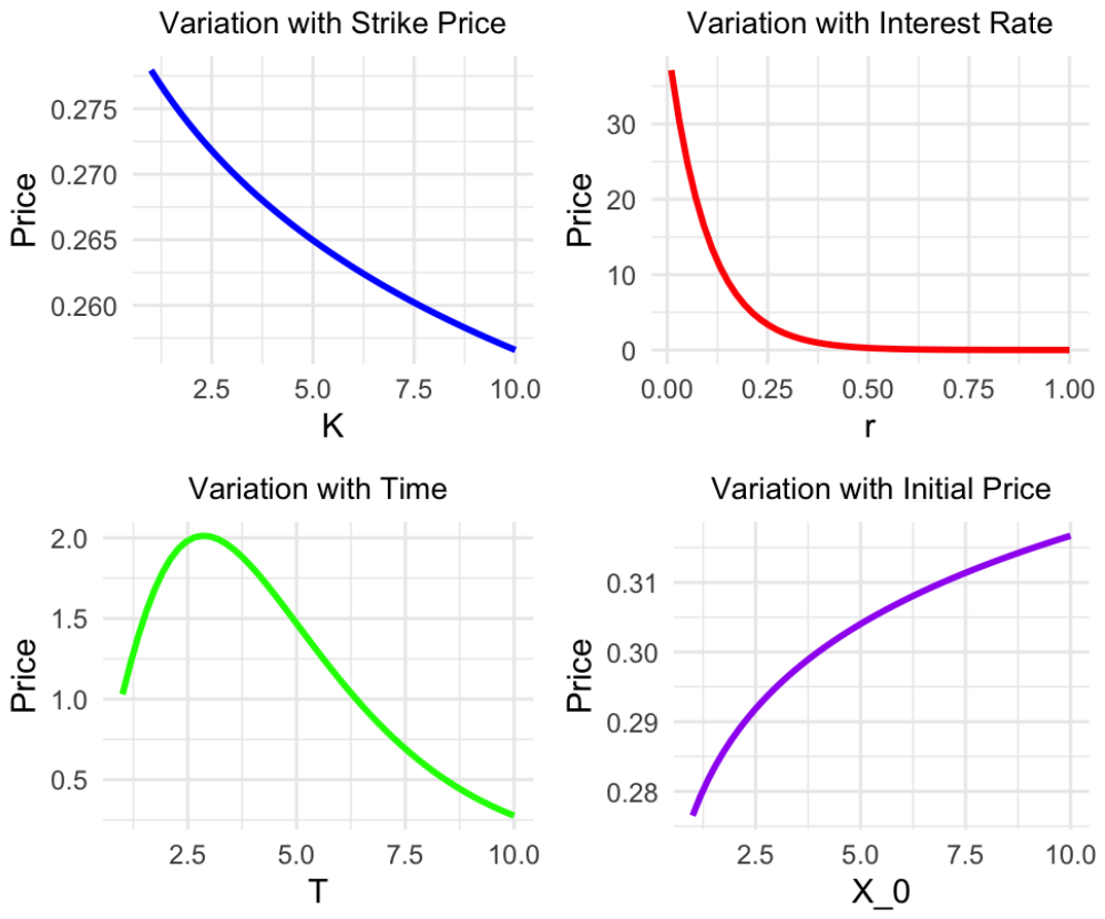
Example 1. Let , , , , , and . The price of a geometric average Asian call option with is .
Figure 1 illustrates the relationships between
and the parameters
K,
r,
T, and
.
4. Geometric Average Asian Put Option Pricing
Mirroring the call derivation, we obtain the put formula by reversing the payoff direction. The derivation confirms the robustness of the -path approach across payoff structures.
Definition 4. A geometric average Asian put option
gives the holder the right to sell the underlying asset at the geometric average price. With fixed strike price K and expiration time T, the payoff at T isBy the fair price principle, the geometric average Asian put option price is Theorem 4. Under Model (
1)
, the geometric average Asian put option price is Proof. Since
is a decreasing function of
, its inverse uncertainty distribution at level
uses the
-quantile of
, i.e.,
Note that
according to the antisymmetry of the logistic function, and substituting
in the integration variable gives (
4). □
Theorem 5. Under Model (
1)
, the geometric average Asian put option price satisfies the following: - 1.
is strictly increasing in K;
- 2.
is strictly decreasing in r;
- 3.
is strictly decreasing in T;
- 4.
is strictly decreasing in .
Proof. The proofs are analogous to those of Theorem 3 with the payoff sign reversed. For Property 1, . For Property 4, since the geometric average is increasing in , making the put payoff decreasing. □
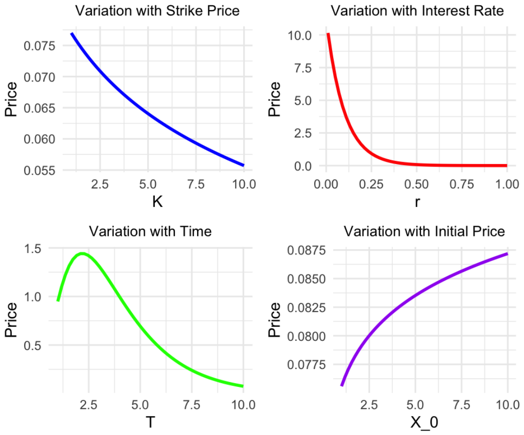
Example 2. Let , , , , , and . The price of a geometric average Asian put option with is .
Figure 2 illustrates the relationships between
and
K,
r,
T, and
.
5. Arithmetic Average Asian Call Option Pricing
Arithmetic averaging is more realistic in practice but does not admit a simple closed form for the average distribution. The -path device nevertheless delivers a tractable representation: the pricing formula reduces to a double integral that is efficiently computable by numerical quadrature.
Definition 5. An arithmetic average Asian call option
gives the holder the right to buy the underlying asset at the arithmetic average price. With fixed strike price K and expiration time T, the payoff at T isBy the fair price principle, the arithmetic average Asian call option price is Theorem 6. Under Model (
1)
, the arithmetic average Asian call option price iswhere is given by (
2)
. Proof. The
-path of the SDE (Model (
1)) is
as in (
2). Since
is continuous and strictly increasing in
for each
t (as
is strictly increasing in
), the time integral
is also strictly increasing in
. By Theorem 2.5 in [
1] (monotone functions of uncertain variables), the inverse uncertainty distribution of
is
Since
is an increasing function of
, its inverse uncertainty distribution is
Applying the expectation formula gives (
5). □
Theorem 7. Under Model (
1)
, the arithmetic average Asian call option price satisfies the following: - 1.
is strictly decreasing in K;
- 2.
is strictly decreasing in r;
- 3.
first increases then decreases in T;
- 4.
is strictly increasing in .
Proof. Property 3. By the Leibniz rule,
For
,
is strictly increasing in
t, so the second term is positive and dominates for small
T; for large
T, the discount factor and the first term dominate, producing a unique maximum.
Property 4.
since
. □
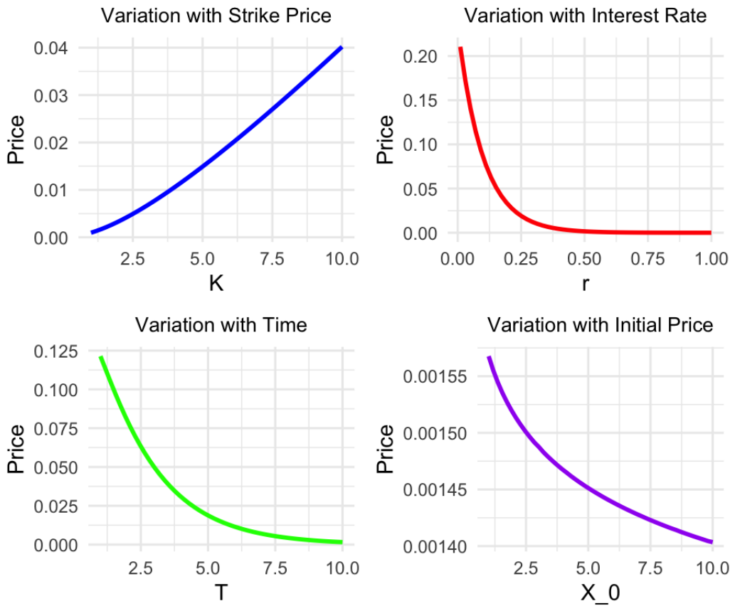
Example 3. Let , , , , , and . The price of an arithmetic average Asian call option with is .
Figure 3 illustrates the relationships between
and
K,
r,
T, and
6. Arithmetic Average Asian Put Option Pricing
The arithmetic average put completes the quartet of Asian option formulas. The derivation follows from the decreasing monotonicity of the put payoff, and the symmetry with the call case underscores the versatility of the -path method.
Definition 6. An arithmetic average Asian put option
gives the holder the right to sell the underlying asset at the arithmetic average price. With fixed strike price K and expiration time T, the payoff at T isBy the fair price principle, the arithmetic average Asian put option price is Theorem 8. Under Model (
1)
, the arithmetic average Asian put option price iswhere is given by (
2)
. Proof. Since
is a
decreasing function of
, its inverse uncertainty distribution at level
uses the
-quantile:
Substituting
and integrating over
give (
6). □
Theorem 9. Under Model (
1)
, the arithmetic average Asian put option price satisfies the following: - 1.
is strictly increasing in K;
- 2.
is strictly decreasing in r;
- 3.
is strictly decreasing in T;
- 4.
is strictly decreasing in .
Proof. Property 3. For
the map
is strictly increasing, so
is strictly increasing in
T. Consequently
is strictly decreasing in
T, and combined with the strictly decreasing discount factor
, we obtain
□
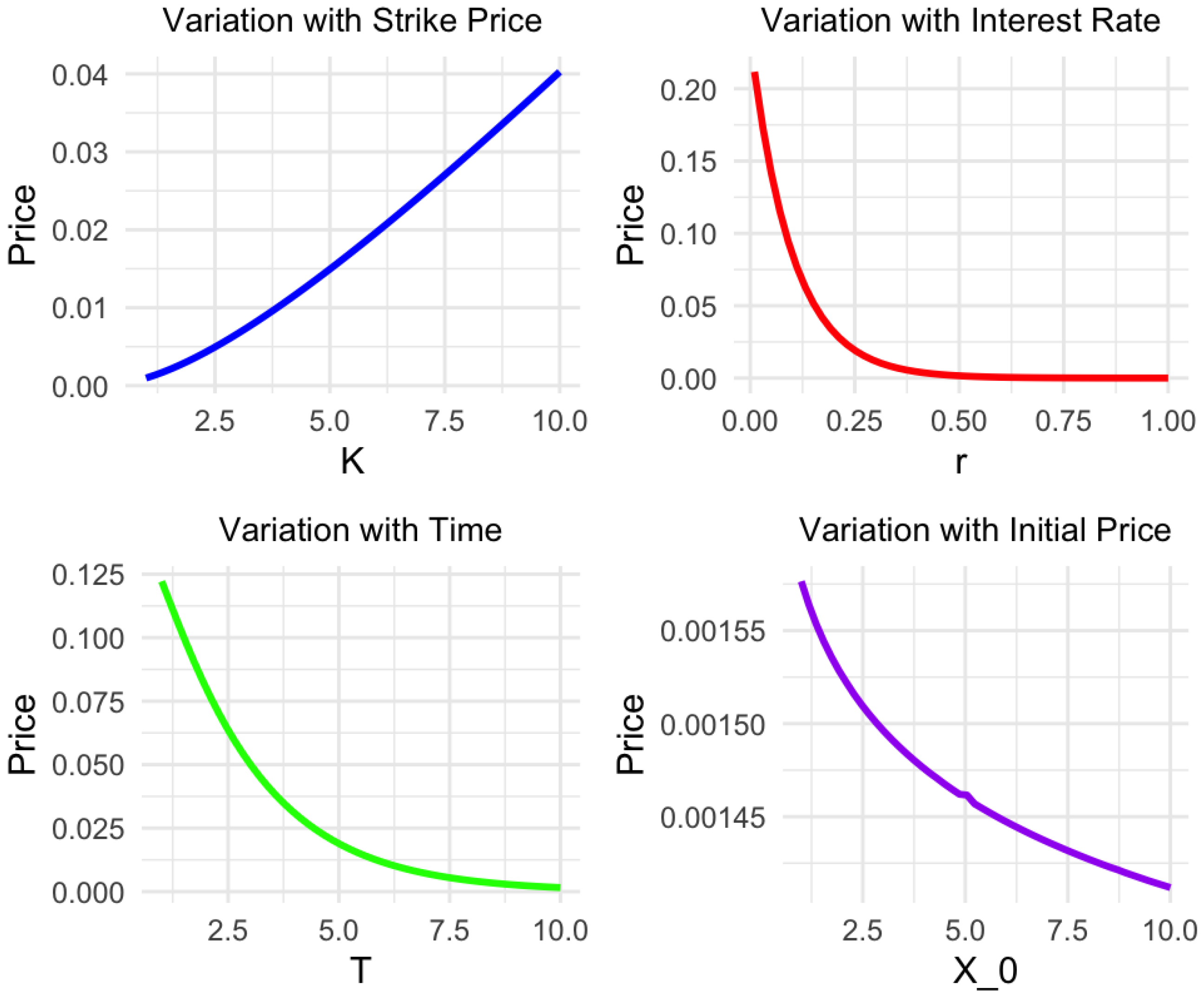
Example 4. Let , , , , , and . The price of an arithmetic average Asian put option with is .
Figure 4 illustrates the relationships between
and
K,
r,
T, and
.
7. Discussion: Option Greeks and Model Comparison
Building upon the pricing formulas derived in
Section 3,
Section 4,
Section 5 and
Section 6, this section provides additional insights into the model through three complementary analyses: option Greeks, the role of the credibility integral, and a comparative model discussion.
7.1. Option Greeks
The “Greeks” measure the sensitivity of an option price to changes in market parameters and are essential tools for hedging. We derive the Greeks for the geometric average Asian call option as a representative case; analogous expressions hold for the other three variants.
From Theorem
3 the call price can be written as
where we introduce two auxiliary functions for notational clarity:
with
. The integrand
vanishes whenever
, so the indicator
appears in all Greek formulas below.
Delta (
) indicates sensitivity to the initial stock price
. Differentiating under the integral sign gives
Since
(because
for
), the geometric average decreases as
increases, so
: higher initial prices raise the effective average relative to
K, making exercise less likely. This reflects the mean-reversion effect: the call option behaves like a short position in the underlying when
.
Rho (
) indicates sensitivity to the risk-free interest rate
r. Only the discount factor
depends on
r, so
which is negative because the integrand is always non-negative and
. An increase in
r reduces the present value of the option payoff, as expected.
Theta (
) indicates sensitivity to the time to expiration
T. Two terms contribute: the derivative of the discount factor and the
T-dependence of
. Writing
, we have
so that
The first term is always negative; the second term changes sign with
T, so
can be positive for short maturities and negative for long maturities, with a unique zero-crossing at
(see Property 3 of Theorem 3).
Vega (
) indicates sensitivity to the diffusion coefficient
. Only
depends on
, so
and by the chain rule
Since
can be positive or negative depending on
and
only filters the in-the-money credibility levels, the sign of
is generally ambiguous and must be determined numerically;
Table 2 illustrates this.
Table 2 reports the numerical values of all four Greeks for the base case of
,
,
,
,
,
, and
, computed via 500-point Gauss–Legendre quadrature of the exact integral formulas above. The Python 3.12.2 script used for all computations is available from the authors upon request.
The Vega is positive, indicating that an increase in the diffusion coefficient raises the call price—the familiar volatility effect. The negative Rho confirms that higher interest rates reduce the option value. The negative Delta reflects mean reversion: when rises, the process has less room to drift upward, so the call’s effective in-the-money probability falls.
7.2. Role of the Credibility Integral
The pricing formulas are expressed as , aggregating over all credibility levels . Each defines an -path scenario: the stock price evolves exactly along with credibility . The integral thus plays the role of a credibility-weighted expectation, analogous to the risk-neutral expectation in the probabilistic framework. Notably,
For call options, the integrand is increasing in (since is increasing in , which in turn is increasing in ), so higher credibility levels (more optimistic scenarios) contribute more to the call price.
For put options the reverse holds: lower credibility levels (more pessimistic scenarios) dominate.
The parameter is an index of belief about future price trajectories, and the integral aggregates expert opinions in the same way that a probability measure aggregates scenarios in the B–S framework.
7.3. Model Comparison
Table 3 summarizes the qualitative differences between three models for Asian option pricing: the Black–Scholes (B–S) model, Liu’s uncertain stock model (LSM), and the uncertain exponential O–U model (this paper).
In the exponential O–U model, the long-run equilibrium depends on the belief level via ; this belief-dependence is the essential departure from both the B–S model and Liu’s model, and it is the mathematical source of the credibility integral in the pricing formula.
8. Conclusions
In this paper, based on uncertainty theory, we have investigated pricing formulas for geometric average and arithmetic average Asian call and put options under the uncertain exponential Ornstein–Uhlenbeck stock model. By means of the -path technique from uncertain calculus, we derived closed-form integral pricing formulas for all four option variants and rigorously proved their monotonicity properties with respect to the strike price, interest rate, time to expiration, and initial stock price. We further computed the option Greeks (Delta, Rho, Theta, and Vega) for the geometric average call option and provided a comparative discussion against Liu’s standard uncertain stock model and the Black–Scholes framework, demonstrating that mean reversion has a quantitatively significant impact on option prices. The formulas developed here are directly applicable to commodity markets and other settings where mean-reverting price behavior is documented.
Author Contributions
Conceptualization, Z.J. and X.Y.; methodology, Z.J.; software, Z.J.; validation, Z.J. and X.Y.; formal analysis, Z.J.; investigation, Z.J.; resources, X.Y.; data curation, Z.J.; writing—original draft preparation, Z.J.; writing—review and editing, X.Y.; visualization, Z.J.; supervision, X.Y.; project administration, X.Y.; funding acquisition, X.Y. All authors have read and agreed to the published version of the manuscript.
Funding
This research was funded by the Fundamental Research Funds for the Directly Affiliated Universities of Inner Mongolia Autonomous Region, grant number BR230903. This research was also supported by the Inner Mongolia Autonomous Region Fifth National Economic Census Research Project, grant number NMJJPC25.
Institutional Review Board Statement
Not applicable.
Informed Consent Statement
Not applicable.
Data Availability Statement
The original contributions presented in this study are included in the article. Further inquiries can be directed to the corresponding author.
Acknowledgments
The authors would like to thank the Department of Mathematics at Inner Mongolia Agricultural University for providing academic support. They also extend their gratitude to colleagues and reviewers for their valuable comments and suggestions, which substantially improved this manuscript. During the preparation of this manuscript the authors used Deepseek-V3 for language polishing. The authors have reviewed and edited the output and take full responsibility for the content of this publication.
Conflicts of Interest
The authors declare no conflicts of interest. The funders had no role in the design of the study; in the collection, analyses, or interpretation of data; in the writing of the manuscript; or in the decision to publish the results.
Abbreviations
The following abbreviations are used in this manuscript:
| UDE | Uncertain differential equation |
| IUD | Inverse uncertainty distribution |
| O–U | Ornstein–Uhlenbeck |
| LSM | Liu’s uncertain stock model |
| B–S | Black–Scholes |
References
- Liu, B. Uncertainty Theory, 2nd ed.; Springer: Berlin/Heidelberg, Germany, 2007. [Google Scholar] [CrossRef] [Scilit]
- Liu, B. Uncertainty Theory: A Branch of Mathematics for Modeling Human Uncertainty; Springer: Berlin/Heidelberg, Germany, 2010. [Google Scholar]
- Chen, X. American option pricing formula for uncertain financial market. Int. J. Oper. Res. 2011, 8, 27–32. [Google Scholar]
- Dai, L.; Fu, Z.; Huang, Z. Option pricing formulas for uncertain financial market based on the exponential Ornstein–Uhlenbeck model. J. Intell. Manuf. 2015, 28, 597–604. [Google Scholar] [CrossRef] [Scilit]
- Chen, X.; Gao, J. Uncertain term structure model of interest rate. Soft Comput. 2013, 17, 597–604. [Google Scholar] [CrossRef] [Scilit]
- Chen, X.; Liu, Y.; Ralescu, D. Uncertain stock model with periodic dividends. Fuzzy Optim. Decis. Mak. 2013, 12, 111–123. [Google Scholar] [CrossRef] [Scilit]
- Peng, J.; Yao, K. A new option pricing model for stocks in uncertainty markets. Int. J. Oper. Res. 2011, 8, 18–26. [Google Scholar]
- Yao, K. No-arbitrage determinant theorems on mean-reverting stock model in uncertain market. Knowl.-Based Syst. 2012, 35, 259–263. [Google Scholar] [CrossRef] [Scilit]
- Sun, Y.; Yao, K.; Fu, Z. Interest rate model in uncertain environment based on exponential Ornstein–Uhlenbeck equation. Soft Comput. 2018, 22, 3865–3873. [Google Scholar] [CrossRef] [Scilit]
- Liu, B. Theory and Practice of Uncertain Programming, 2nd ed.; Springer: Berlin/Heidelberg, Germany, 2009. [Google Scholar] [CrossRef] [Scilit]
- Liu, B.; Chen, X. Uncertain multiobjective programming and uncertain goal programming. J. Uncertain. Anal. Appl. 2015, 3, 10. [Google Scholar] [CrossRef] [Scilit]
- Liu, B.; Yao, K. Uncertain multilevel programming: Algorithm and applications. Comput. Ind. Eng. 2015, 89, 235–240. [Google Scholar] [CrossRef] [Scilit]
- Gao, R.; Yao, K. Importance index of component in uncertain reliability system. J. Uncertain. Anal. Appl. 2016, 4, 7. [Google Scholar] [CrossRef] [Scilit]
- Liu, B. Uncertain risk analysis and uncertain reliability analysis. J. Uncertain Syst. 2010, 4, 163–170. [Google Scholar]
- Liu, B. Some research problems in uncertainty theory. J. Uncertain Syst. 2009, 3, 3–10. [Google Scholar]
- Yao, K.; Chen, X. A numerical method for solving uncertain differential equations. J. Intell. Fuzzy Syst. 2013, 25, 825–832. [Google Scholar] [CrossRef] [Scilit]
- Liu, B. Fuzzy process, hybrid process and uncertain process. J. Uncertain Syst. 2008, 2, 3–16. [Google Scholar]
| Disclaimer/Publisher’s Note: The statements, opinions and data contained in all publications are solely those of the individual author(s) and contributor(s) and not of MDPI and/or the editor(s). MDPI and/or the editor(s) disclaim responsibility for any injury to people or property resulting from any ideas, methods, instructions or products referred to in the content. |