On Simple EM Acceleration Schemes Suitable for Mixture Modelling with High Overlap Between Components

Abstract

The Expectation-Maximisation (EM) algorithm is widely used for maximum likelihood estimation in incomplete data problems such as mixture modelling, but it often converges slowly, particularly when mixture components overlap substantially. This study presents a comprehensive empirical evaluation of simple EM acceleration schemes for Gaussian mixture models, comparing linear (STEM), quadratic (SQUAREM), and greedy (line search, golden section) methods across 240 simulated mixture configurations spanning three dimensionalities, four component counts, five overlap levels, and four sample sizes. A key contribution is the first systematic comparison of the three acceleration parameter estimates (${\alpha }_1$, ${\alpha }_2$, ${\alpha }_3$) in the mixture modelling context: we show that only ${\alpha }_3$, which is derived as the geometric mean estimate of ${\alpha }_1$ and ${\alpha }_2$, provides genuine acceleration, while ${\alpha }_1$ and ${\alpha }_2$ consistently increase iteration counts by 50–110% relative to ${\alpha }_3$, effectively acting as deceleration. With ${\alpha }_3$, SQUAREM reduces iterations by up to 48% with negligible computational overhead, while greedy methods achieve similar iteration reductions but at 50–110% greater wall-clock time due to repeated log-likelihood evaluations. Crucially, acceleration does not degrade parameter estimation quality under any tested combination of initialisation, overlap, dimensionality, or number of components. We further examine the interaction between acceleration and initialisation, finding that k-means benefits most from acceleration (up to 50% time savings), while the REBMIX (Rough-Enhanced-Bayes MIXture estimation) algorithm benefits least as it already starts near the optimum. Among REBMIX configurations, histogram preprocessing with the outliers mode traversing strategy offers the best trade-off between quality and computational cost. The findings are validated on a real-world Backblaze hard drive failure dataset, confirming the practical utility of EM acceleration. All methods are implemented in the free and open-source R package rebmix, accompanied by full source code.

1. Introduction

The Expectation-Maximisation (EM) algorithm [1] is one of the most useful and widely adopted algorithms in data science, statistics, and pattern recognition. It is best known for its role as a maximum likelihood estimator in the presence of missing or incomplete data [2]. The EM algorithm has a broad range of applications, the most prominent being mixture model parameter estimation, with further use in clustering [3,4], image segmentation [5], density estimation [6,7], regression [8], anomaly detection [9] and more.

EM’s popularity lies in its simplicity and stability [2]. It addresses otherwise intractable maximum likelihood estimation problems involving missing data through an iterative procedure consisting of an Expectation (E) step and a Maximisation (M) step, repeated until convergence. At each iteration, the algorithm guarantees an increase in the likelihood function, making it a strictly hill-climbing method [10]. Nevertheless, due to the presence of multiple local optima in the likelihood surface, EM requires a reasonably good initialisation [11]. The choice of the starting point can significantly influence the convergence path and ultimately determine which local optimum the algorithm converges to. The initialisation of EM has been extensively studied, and a variety of methods have been proposed to address this issue effectively [12,13,14,15].

Another limitation of the EM algorithm is its slow, linear convergence to the optimum of the likelihood function [10]. Although this linear convergence contributes to EM’s stability, it often requires a large number of iterations to closely approach the optimum. This limitation can be partially addressed by using better initialisation methods, but it remains a significant concern in practice [16]. The issue becomes even more pronounced in scenarios where the updates in the E-step are minimal, or in other words, when the data poorly separates the latent components and the estimated entropy of their posterior distribution remains high [2]. In such cases, obtaining a reasonable initialisation is particularly challenging due to the high degree of overlap in the data [17]. Additionally, some distributions do not have closed-form solutions, and iterative procedures are required to obtain the M-step updates [18]. Therefore, accelerated EM approaches should be explored, and their effects carefully evaluated.

In this paper, simple yet effective approaches to accelerate the EM algorithm are reviewed and empirically investigated. A related study by [19] compared acceleration techniques for the EM algorithm in the context of item response theory models; the present work focuses instead on mixture model estimation with varying degrees of overlap between components, examining how overlap influences the performance and stability of different acceleration schemes. The primary objective is to establish clear guidelines on when EM acceleration is most effective, to identify which methods perform best under different conditions, and to examine how different initialisation strategies influence the stability and effectiveness of acceleration. A key finding, which to our knowledge has not been previously documented for mixture modelling, is that only one of the three acceleration parameter estimates proposed by [10] provides genuine acceleration; the other two consistently act as deceleration. To achieve this, a comprehensive simulation study was designed to incorporate a wide range of factors, including the degree of overlap between mixture components, the number of dimensions, the number of components in the model, the size of the data set, and other relevant parameters. These factors significantly affect the complexity of the estimation task and are therefore essential for evaluating the performance of various acceleration schemes. The study includes approximately 2400 distinct data sets, making it, to the best of our knowledge, one of the most extensive investigations on this topic. In addition, multiple estimation strategies based on different EM initialisation methods are considered. Finally, the empirical findings are validated using a real-world data set to demonstrate their practical relevance and general applicability.

The outline of this article is as follows. Section 2 provides the theoretical background on mixture modelling and the EM algorithm. Section 3 presents a review of the acceleration schemes considered in this work. Section 4 offers a brief overview of EM initialisation strategies. Section 5 introduces the experimental setup used to evaluate the performance of different acceleration schemes. Section 6 reports the main results and discussion based on simulated data sets. Section 7 presents real-world data set along with the corresponding results. The article concludes with Section 8.

2. Theoretical Background

2.1. Prerequisites

Let $\mathit{Y}=\{{\mathit{y}}_1,{\mathit{y}}_2,\dots ,{\mathit{y}}_n\}$ be a d-dimensional observed data set of n continuous observations. Let $\mathit{Y}$ be generated by a c-component mixture distribution. Each observation ${\mathit{y}}_j=\{y_1,y_2,\dots ,y_d\}$ thus follows the probability density function (PDF) in form of

$$f\left({\mathit{y}}_j\right|c,\mathit{w},\mathit{\Theta })=\sum _{l=1}^c{w}_l{f}_l\left({\mathit{y}}_j\right|{\mathit{\Theta }}_l).$$

(1)

Mixture distribution (i.e., mixture model) is composed of c weighted components. Each component, denoted by the subscript l, follows a simple parametric probability distribution, with PDF denoted by $f_l$, such as a Gaussian distribution and similar [2], and is parametrised by ${\mathbf{\Theta }}_l$. For example, for multivariate normal mixture model, each component follows multivariate Gaussian distribution $N_l\left({\mathit{y}}_j\right|{\mathit{\mu }}_l,{\mathbf{\Sigma }}_l)$, parametrised with mean values ${\mathit{\mu }}_l$ and covariance matrices ${\mathbf{\Sigma }}_l$. The weights $w_l$ of each component have the properties of the convex combination $w_l\ge 0$ and ${\sum }_{l=1}^c{w}_l=1$ [2]. For convenience in further, we will arrange the mixture model parameters in a vector $\mathbf{\Theta }$

$$\mathbf{\Theta }=\{w_1,w_2,\dots ,w_c,{\mathit{\Theta }}_1,{\mathit{\Theta }}_2,\dots ,{\mathit{\Theta }}_c\}=\{\mathit{w},\mathit{\Theta }\}.$$

(2)

2.2. Parameter Estimation

Parameter estimates are usually obtained with maximum likelihood. The estimation can be written as

$$\widehat{\mathbf{\Theta }}=\underset{\mathbf{\Theta }}{\mathrm{argmax}}logL\left(\mathit{Y}\right|\mathbf{\Theta }),$$

(3)

where

$$logL\left(\mathit{Y}\right|\mathbf{\Theta })=\sum _{j=1}^{n}log\left(\sum _{l=1}^c{w}_l{f}_l\left({\mathit{y}}_j\right|{\mathit{\Theta }}_l)\right),$$

(4)

is the log likelihood function.

The solution to the maximisation problem in Equation (3) poses a challenge, as the likelihood values tend to increase with the number of components c, resulting in overfitting. Therefore, maximising the log-likelihood should be done with a known value of c. When the number of components in the mixture model is unknown, it is necessary to apply a model selection procedure to prevent overfitting. The best model is typically selected using an information criterion that penalizes the log-likelihood based on model complexity (number of components c) [20].

2.3. Expectation-Maximisation Algorithm

The EM algorithm is the standard method for obtaining maximum likelihood parameter estimates for mixture models [2]. It is commonly used in model selection procedures to estimate parameters for a specified number of components c [21]. As a hill-climbing optimization algorithm, EM alternates between the E step, which estimates the expected value of the log-likelihood given the current model parameters, and the M step, which updates the parameters to maximise this expectation. This process continues iteratively until the algorithm converges to a local optimum of the log-likelihood function.

In the E step of the algorithm, the posterior probability ${\tau }_{lj}$ that the observation ${\mathit{y}}_j$ from $\mathit{Y}$ arose from the l-th component is calculated   

$${\tau }_{lj}^{(t+1)}={\displaystyle \frac{w_l^{\left(t\right)}{f}_l\left({\mathit{y}}_j\right|{\mathit{\mu }}_l^{\left(t\right)},{\mathit{\Sigma }}_l^{\left(t\right)})}{{\sum }_{\tilde{l}=1}^c{w}_{\tilde{l}}^{\left(t\right)}{f}_{\tilde{l}}\left({\mathit{y}}_j\right|{\mathit{\mu }}_{\tilde{l}}^{\left(t\right)},{\mathit{\Sigma }}_{\tilde{l}}^{\left(t\right)})}}.$$

(5)

In the M step the iteration-wise update equations for the parameters can be derived by maximisation of conditional expectation of the complete-data log-likelihood function [2]. The updates of the parameters for the Gaussian mixtures can be obtained with following equations. The weights $w_l$ with

$$w_l^{(t+1)}={\displaystyle \frac{{\sum }_{j=1}^n{\tau }_{lj}^{(t+1)}}{n}},$$

(6)

the mean vectors ${\mathit{\mu }}_l$ with

$${\mathit{\mu }}_l^{(t+1)}={\displaystyle \frac{{\sum }_{j=1}^n{\tau }_{lj}^{(t+1)}{\mathit{y}}_j}{{\sum }_{j=1}^n{\tau }_{lj}^{(t+1)}}},$$

(7)

and the covariance matrices ${\mathit{\Sigma }}_l$ with update equation

$${\mathit{\Sigma }}_l^{(t+1)}={\displaystyle \frac{{\sum }_{j=1}^n{\tau }_{lj}^{(t+1)}({\mathit{y}}_j-{\mathit{\mu }}_l^{(t+1)}){({\mathit{y}}_j-{\mathit{\mu }}_l^{(t+1)})}^T}{{\sum }_{j=1}^n{\tau }_{lj}^{(t+1)}}}.$$

(8)

3. Acceleration Schemes

The EM iteration can be simply viewed as a mapping $F:{\mathbb{R}}^{|\mathbf{\Theta }|}\to {\mathbb{R}}^{|\mathbf{\Theta }|}$ where

$${\mathbf{\Theta }}^{t+1}=F\left({\mathbf{\Theta }}^t\right)$$

(9)

and the parameter iteration update can be calculated as

$$\Delta {\mathbf{\Theta }}^t=F\left({\mathbf{\Theta }}^t\right)-{\mathbf{\Theta }}^t,$$

(10)

thus the iterative scheme can generally be expressed as

$${\mathbf{\Theta }}^{t+1}={\mathbf{\Theta }}^t+\Delta {\mathbf{\Theta }}^t.$$

(11)

The EM algorithm is known to exhibit slow convergence [22]. In this section we will further review two simple interesting acceleration schemes provided in [10].

3.1. Acceleration with Linear Scheme

The first scheme, named STEM in [10], to accelerate the EM algorithm can be simply written as

$${\mathbf{\Theta }}^{t+1}={\mathbf{\Theta }}^t+\alpha \Delta {\mathbf{\Theta }}^t,$$

(12)

where the parameter $\alpha$ can be viewed as the learning rate and controls the speed of convergence. Specifically, $\alpha >1$ accelerates the convergence, while $\alpha <1$ decelerates it. Too high a value of $\alpha$ can cause unwanted oscillations in the parameter estimates in each iteration, while lower values may not help with slow convergence.

3.2. Acceleration with Quadratic Scheme

The second scheme, also named SQUAREEM in [10], uses two EM iterations to obtain the final update of parameter estimates, i.e.,

$${\mathbf{\Theta }}^{t+2}={\mathbf{\Theta }}^t+2\alpha \Delta {\mathbf{\Theta }}^t+{\alpha }^2(\Delta {\mathbf{\Theta }}^{t+1}-\Delta {\mathbf{\Theta }}^t)$$

(13)

where

$$\Delta {\mathbf{\Theta }}^t=F\left({\mathbf{\Theta }}^t\right)-{\mathbf{\Theta }}^t$$

(14)

and

$$\Delta {\mathbf{\Theta }}^{t+1}=F\left({\mathbf{\Theta }}^{t+1}\right)-{\mathbf{\Theta }}^{t+1}=F\left(F\left({\mathbf{\Theta }}^t\right)\right)-F\left({\mathbf{\Theta }}^t\right)$$

(15)

Again, same remarks concerning acceleration parameter $\alpha$ made in previous section apply here. When $\alpha =1$ the Equation (13) becomes standard EM update and when $\alpha \ne 1$ the convergence can be improved. Also, according to [10] this scheme can converge faster than both standard EM update and linear acceleration scheme.

3.3. Acceleration Parameter Estimation

Choosing right value for acceleration parameter in Equations (12) and (13) can be quite challenging. In that manner we will review 3 different strategies in the text to follow.

The first and simplest strategy is to use a fixed value for the acceleration parameter $\alpha$, such as $\alpha =1.5$. While this approach can be effective, it has two key limitations. First, the choice of the parameter must be determined beforehand, and second, the parameter remains constant throughout the optimization process, which can potentially lead to suboptimal parameter estimates and hinder convergence. This strategy is more interpretable when applied alongside a linear acceleration scheme, i.e., Equation (12). If the EM optimization trajectory approximates a linear curve, the fixed value of $\alpha$ can be justified in a straightforward manner. Essentially, this approach increases the gradient step size in a manner analogous to successive over-relaxation methods.

The second strategy, a greedy approach, employs a search algorithm such as line search or golden section search—to determine the optimal value of $\alpha$ at each iteration. By using the log-likelihood function as the optimization criterion, this method maximises the log-likelihood and ensures the largest possible update along the linear trajectory during each iteration. The key difference between line search and golden section search lies in their search ranges and computational complexity. Line search is well-suited for narrower ranges of $\alpha$, such as $\alpha \in (1,2)$, and has linear time complexity. In contrast, golden section search can explore a wider range of values, such as $\alpha \in (1,5)$, due to its logarithmic time complexity, making it more efficient for broader parameter searches.

The third strategy focuses on optimizing a measure of discrepancy between two consecutive updates, ${\mathbf{\Theta }}^{t+1}$ and ${\mathbf{\Theta }}^t$, as highlighted in [10]. This approach yields three distinct estimates for the parameter $\alpha$

$${\alpha }_1=-{\displaystyle \frac{r_n^T{v}_n}{v_n^T{v}_n}},{\alpha }_2=-{\displaystyle \frac{r_n^T{r}_n}{r_n^T{v}_n}},{\alpha }_3={\displaystyle \frac{\left|\right|r_n\left|\right|}{\left|\right|v_n\left|\right|}},$$

(16)

where $r_n=\Delta {\Theta }^t$ and $v_n=\Delta {\Theta }^{t+1}-\Delta {\Theta }^t$. The first estimate, ${\alpha }_1$, is derived by minimizing the squared L2 norm, $\left|\right|{\mathbf{\Theta }}^{t+1}-{\mathbf{\Theta }}^t{\left|\right|}^2$. The second estimate, ${\alpha }_2$, comes from optimizing $\left|\right|{\mathbf{\Theta }}^{t+1}-{\mathbf{\Theta }}^t{\left|\right|}^2/{\alpha }^2$, while the third estimate, ${\alpha }_3$, is obtained by optimizing $\left|\right|{\mathbf{\Theta }}^{t+1}-{\mathbf{\Theta }}^t{\left|\right|}^2/\alpha$. Alongside the first strategy, this strategy is highly effective, particularly when factoring in the additional computational overhead required for its implementation.

4. Initialisation of EM

The EM algorithm requires a set of initial parameters. This set dictates many aspects, most importantly the quality of the final parameter estimates, as the log-likelihood function has many local optima. Poorly chosen initial parameters can lead to convergence to spurious local optima or even degenerate estimates. As a result, there is a vast body of literature concerning the initialisation of the EM algorithm [14].

In a recent study [17] reviewed several initialisation methods, including random initialisation, k-means, hierarchical clustering, and the REBMIX algorithm. Their findings suggest that different initialisation methods are better suited to different scenarios. For example, REBMIX performs well when there is a low degree of overlap between mixture model components, whereas k-means is more robust to overlap.

Additionally, various authors often recommend using multiple EM initialisations along with a simple voting mechanism to select the initial parameter estimates [11]. A common procedure, known as small EM, involves a large number of random initialisations combined with short EM runs (a few iterations) to identify the best initial parameter estimates—i.e., those yielding the highest likelihood [16]. Since this approach accumulates a substantial number of EM iterations across restarts, it stands to benefit considerably from acceleration.

5. Experimental Setup

To evaluate the performance of different acceleration schemes under controlled conditions, we designed a simulation study using the R version 4.3.3 MixSim package [23]. MixSim enables the generation of Gaussian mixture model parameters with a prescribed level of pairwise overlap between components, allowing systematic control over the difficulty of the estimation problem.

5.1. Simulation Design

MixSim supports two types of overlap specification: average overlap ($\overline{\omega }$), which controls the mean pairwise overlap across all component pairs, and maximum overlap (${\omega }_{max}$), which sets the overlap of the most overlapping pair. In this study, we use average overlap exclusively. This choice simplifies the experimental design while still capturing both distributed and concentrated overlap scenarios. Specifically, for $c=2$ components, only a single pair exists, so $\overline{\omega }\equiv {\omega }_{max}$ and the average overlap specification is equivalent to maximum overlap. For $c\ge 3$, average overlap distributes the overlap across all component pairs, representing the more challenging and practically common setting in which no single pair dominates the mixture structure.

The simulation parameters are summarised in

Table 1. Design parameters for the simulation study.

Parameter	Symbol	Values
Overlap level	$\delta$	$0.01$, $0.05$, $0.1$, $0.15$, $0.2$
Dimensions	d	3, 5, 10
Components	c	2, 3, 5, 10
Observations	n	200, 400, 800, 1600
Repetitions		10

. For dimensionality, we chose $d\in \{3,5,10\}$, omitting univariate mixtures (which have been extensively studied) and $d=2$ (which produced rankings identical to $d=3$ in preliminary experiments). For the number of components, we chose $c\in \{2,3,5,10\}$, where $c=2$ serves as a natural baseline representing both the simplest mixture and the maximum overlap case, as discussed above. The overlap levels were set to $\delta \in \{0.01,0.05,0.1,0.15,0.2\}$, spanning from near-separation to substantial overlap. Data sets were generated with $n\in \{200,400,800,1600\}$ observations; the smallest size ($n=100$) was excluded based on preliminary analysis showing that acceleration provides negligible benefit below $n=200$. All component weights were set to be equal (balanced). Preliminary experiments confirmed that balanced and imbalanced mixtures produced identical acceleration method rankings, so we report only the balanced case to avoid redundancy. Each unique configuration was replicated 10 times using independent random samples, consistent with standard practice in mixture simulation studies [13,17]. Although 10 replications per configuration may appear modest, the experimental design ensures that all reported results aggregate across multiple design factors: even the most granular results in Table 4 (specific $n\times \delta$) average over $3\times 4\times 4\times 10=480$ independent runs, yielding standard errors below 2 percentage points for all reported reduction values. All figures report ±1 standard error bars, which quantify the remaining Monte Carlo sampling uncertainty. In total, the design comprises $3\times 4\times 5\times 4=240$ unique mixture configurations.

5.2. Estimation Strategies

Each simulated data set was fitted using a combination of initialisation method and EM acceleration scheme. For initialisation, we employed random assignment, k-means clustering, hierarchical clustering (hclust), and the REBMIX algorithm. For REBMIX, we additionally evaluated three preprocessing methods—histogram, kernel density estimation, and k-nearest neighbours—as well as three mode traversing strategies: all, outliers, and outliersplus. Details on preprocessing and mode traversing are given in [24,25].

For the EM stage, we considered five acceleration schemes: (i) standard EM without acceleration, (ii) line search acceleration, (iii) golden section search acceleration, (iv) linear acceleration (STEM), and (v) quadratic acceleration (SQUAREM). The line and golden search approaches estimate $\alpha$ greedily at each iteration by maximising the log-likelihood over a range of candidate values; their implementations are detailed in Appendix A. The STEM and SQUAREM schemes all three $\alpha$ estimates proposed by [10] (${\alpha }_1$, ${\alpha }_2$, and ${\alpha }_3$ from Equation (16)).

Convergence is declared when the per-observation change in log-likelihood falls below a threshold $\epsilon ={10}^{-7}$

$${\displaystyle \frac{|l^{(t+1)}-l^{\left(t\right)}|}{n}}<\epsilon ,$$

(17)

where $l^{\left(t\right)}$ and $l^{(t+1)}$ are the log-likelihood values at consecutive iterations. Normalising by the number of observations n ensures that the convergence criterion is comparable across different sample sizes. The maximum number of iterations was set to 1000.

All estimation strategies were implemented within the rebmix R package, which provides a unified interface for applying different EM acceleration schemes alongside various initialisation methods. To the best of our knowledge, rebmix is the only publicly available R package that natively supports EM acceleration for mixture model estimation. Other well-established packages, such as mclust [3], mixtools, and flexmix implement only the standard EM algorithm without acceleration options. The unaccelerated EM results in this study, therefore, serve as a baseline equivalent to what these packages produce under comparable initialisation and convergence settings. For a comprehensive comparison of R packages for Gaussian mixture modelling, we refer the reader to [17].

The complete set of estimation strategies is summarised in

Table 2. Methods and their variations used for parameter estimation.

Estimation Stage	Methods
Initialisation	Random, k-means, REBMIX, hclust
EM acceleration	Standard 1, line, golden, STEM 2, SQUAREM 3
Strategy	Initialisation + EM

¹ Standard EM without acceleration. ² Linear acceleration with ${\alpha }_3$ estimate. ³ Quadratic acceleration with ${\alpha }_3$ estimate.

.

5.3. Evaluation Metrics

Performance is assessed along two dimensions: estimation quality and computational cost. Since the true mixture parameters are known, we compute the bias and mean squared error (MSE) for each parameter group—weights, means, and covariance matrices—averaged over components and dimensions to ensure comparability across configurations of different sizes. For bias, we report the mean of absolute values. These metrics are formally defined in

Table 3. Metrics used for evaluation of estimation strategies.

Metric	Definition
$b_w$	${\displaystyle \frac{1}{c}}{\sum }_{l=1}^c|E\left(\widehat{w_l}\right)-w_l|$
$b_{\mathit{\mu }}$	${\displaystyle \frac{1}{cd}}{\sum }_{l=1}^c{\sum }_{i=1}^d|E\left({\widehat{\mathit{\mu }}}_{il}\right)-{\mathit{\mu }}_{il}|$
$b_{\Sigma }$	${\displaystyle \frac{1}{cd(d+1)/2}}{\sum }_{l=1}^c{\sum }_{i=1}^d{\sum }_{\tilde{i}=1}^i|E\left({\widehat{\Sigma }}_{i\tilde{i}l}\right)-{\Sigma }_{i\tilde{i}l}|$
${\mathrm{MSE}}_w$	${\displaystyle \frac{1}{c}}{\sum }_{l=1}^{c}E\left({({\widehat{w}}_l-w_l)}^2\right)$
${\mathrm{MSE}}_{\mathit{\mu }}$	${\displaystyle \frac{1}{cd}}{\sum }_{l=1}^c{\sum }_{i=1}^{d}E\left({({\widehat{\mathit{\mu }}}_{il}-{\mathit{\mu }}_{il})}^2\right)$
${\mathrm{MSE}}_{\Sigma }$	${\displaystyle \frac{1}{cd(d+1)/2}}{\sum }_{l=1}^c{\sum }_{i=1}^d{\sum }_{\tilde{i}=1}^{i}E\left({({\widehat{\Sigma }}_{i\tilde{i}l}-{\Sigma }_{i\tilde{i}l})}^2\right)$
$logL$	${\sum }_{j=1}^{n}logf\left({\mathit{y}}_j\right|c,\mathit{w},\widehat{\mathbf{\Theta }})$
ARI	Adjusted Rand Index [26]
Iterations	Number of EM iterations until convergence
Time	Total wall-clock estimation time

.

We additionally report two application-oriented metrics: the estimated log-likelihood, which summarises overall model fit, and the Adjusted Rand Index (ARI) [26], which evaluates clustering quality. These metrics capture whether the estimated model is practically useful even when individual parameter estimates deviate from their true values—a common occurrence under high overlap.

Finally, we report two computational metrics: the number of EM iterations and the total wall-clock estimation time (including initialisation). Both are necessary because a scheme that reduces iterations may still be slower in wall time if each iteration carries additional overhead, as is the case for line and golden search methods.

Note that high log-likelihood values do not always indicate good parameter recovery, as they may reflect spurious solutions with near-singular covariance matrices [2]. Evaluation of estimated parameter quality requires reordering estimated components to match the true components; this was accomplished using a minimum-cost assignment based on the Euclidean distance between true and estimated parameter vectors, solved via the Hungarian algorithm [27].

6. Results and Discussion

In this section we present the results and discussion obtained on simulated datasets.

6.1. Convergence Performance of Acceleration Schemes

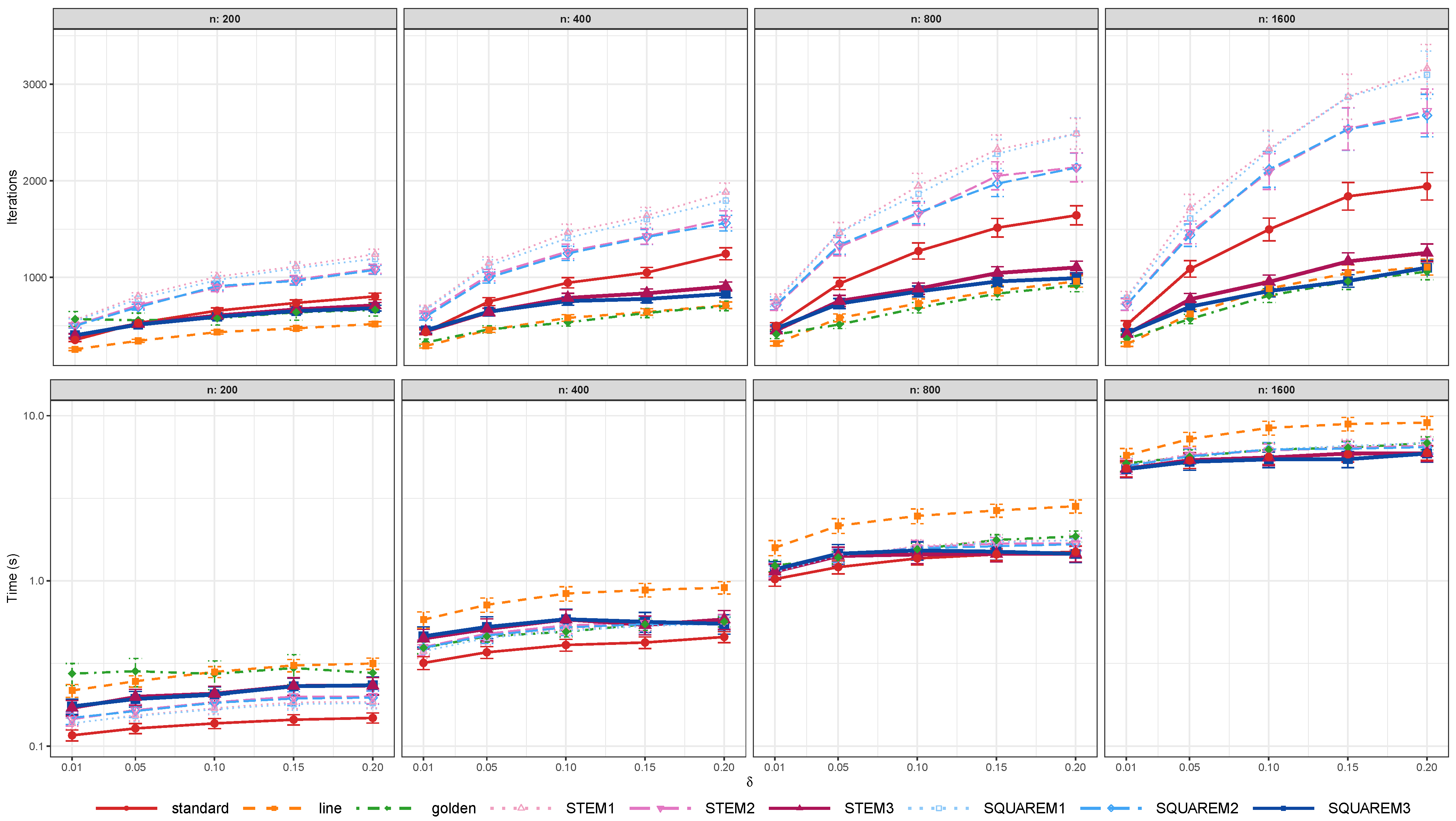
Figure 1 presents the mean number of EM iterations (top row) and computation time (bottom row, log scale) as a function of overlap level $\delta$, faceted by sample size n, for all nine acceleration variants evaluated in this study. The figure reveals three distinct groups of methods.

The first group consists of the ${\alpha }_1$ and ${\alpha }_2$ variants of STEM and SQUAREM. These methods consistently require more iterations than standard EM: STEM with ${\alpha }_1$ requires $105\%$ more iterations than STEM with ${\alpha }_3$, while ${\alpha }_2$ requires $80\%$ more. The pattern is nearly identical for SQUAREM ($+114\%$ and $+90\%$, respectively). Both ${\alpha }_1$ and ${\alpha }_2$ also exceed standard EM in iteration count ($+52$–$55\%$ for ${\alpha }_1$, $+35$–$36\%$ for ${\alpha }_2$), effectively acting as deceleration rather than acceleration. This occurs because ${\alpha }_1$ and ${\alpha }_2$ frequently produce oversized step sizes that fail to increase the log-likelihood, triggering a fallback to an unaccelerated EM update at each such iteration. The ${\alpha }_3$ estimate, being the geometric mean of ${\alpha }_1$ and ${\alpha }_2$, yields a more conservative step size that succeeds more frequently. The quality of the obtained solutions, as measured by ARI, is statistically indistinguishable across all $\alpha$ variants (spread $<0.003$). These findings hold across all overlap levels, sample sizes, and initialisations tested, confirming the recommendation of [10]. In all subsequent analyses, only ${\alpha }_3$ is used for STEM and SQUAREM.

The second group contains the greedy search methods—line search and golden section search. These achieve the largest iteration reductions (up to $40\%$ and $37\%$, respectively), as they explicitly maximise the log-likelihood over a range of $\alpha$ values at each iteration. However, this comes at a substantial computational cost: line search increases total computation time by $53\%$ on average, with increases exceeding $100\%$ at small-to-moderate sample sizes, due to multiple additional log-likelihood evaluations per iteration. Golden section search is less expensive (approximately $14\%$ slower on average) but exhibits erratic behaviour: at $n=200$ and $\delta =0.01$, it requires $62\%$ more iterations than standard EM, and it produced catastrophic numerical instability in a small number of runs, with MSE values for covariance estimates exceeding ${10}^{10}$. Both greedy methods are therefore impractical for routine use despite their iteration efficiency.

The third group comprises STEM and SQUAREM with ${\alpha }_3$, which provides the best trade-off between iteration reduction and computational overhead. SQUAREM reduces iterations by $29\%$ overall, with the benefit increasing monotonically with both overlap and sample size: from a modest $3\%$ at $\delta =0.05$, $n=200$ to $48\%$ at $\delta =0.15$, $n=1600$. STEM follows a similar but slightly less pronounced pattern ($24\%$ overall reduction). At small sample sizes and low overlap, both methods may slightly increase the iteration count (by up to $14\%$ at $n=200$, $\delta =0.01$), indicating that the overhead of computing ${\alpha }_3$ is not offset by the acceleration gain in these easy problems. Crucially, the per-iteration overhead of STEM and SQUAREM is minimal: at $n\ge 800$, both methods achieve wall-clock time savings that match or exceed their iteration savings, while at smaller n the time overhead remains modest.

Table 4 provides detailed iteration and time reduction percentages across the full $n\times \delta$ grid. The monotonic increase of SQUAREM’s benefit with both n and $\delta$ is evident: the method becomes increasingly valuable precisely in the settings where standard EM struggles most.

Table 4. Percentage reduction in EM iterations and computation time relative to standard EM (%). Positive values indicate improvement; negative values indicate degradation.

n	Method	Metric	Overlap Level $\mathit{\delta }$
			0.01	0.05	0.10	0.15	0.20
200	Line	Iterations	27.5	35.0	33.9	35.8	40.1
		Time	−86.0	−92.2	−104.2	−112.3	−112.7
	Golden	Iterations	−61.5	−5.3	12.1	13.1	16.8
		Time	−135.4	−121.1	−98.6	−104.6	−86.4
	STEM	Iterations	−11.7	2.0	7.7	9.1	11.6
		Time	−46.8	−54.8	−50.7	−59.3	−56.4
	SQUAREM	Iterations	−13.7	3.2	9.6	11.5	15.2
		Time	−49.7	−50.7	−49.2	−58.5	−57.0
400	Line	Iterations	33.2	39.1	38.5	38.9	45.1
		Time	−82.9	−93.9	−105.0	−108.1	−99.0
	Golden	Iterations	24.8	38.4	43.5	39.8	41.8
		Time	−23.6	−24.9	−20.3	−28.9	−23.8
	STEM	Iterations	−1.9	14.5	16.6	20.5	27.2
		time	−40.7	−38.4	−42.8	−27.8	−27.7
	SQUAREM	Iterations	−4.4	13.9	20.1	26.0	33.3
		Time	−45.0	−42.4	−43.2	−33.5	−20.1
800	Line	Iterations	36.6	38.0	42.6	43.0	42.9
		Time	−55.0	−78.2	−80.9	−84.7	−89.0
	Golden	Iterations	17.7	45.3	46.1	45.1	40.0
		Time	−20.6	−14.3	−13.5	−22.3	−24.1
	STEM	Iterations	9.0	19.2	30.6	31.0	32.9
		Time	−11.1	−16.8	−5.6	−0.8	2.4
	SQUAREM	Iterations	5.2	22.1	32.9	36.7	39.6
		Time	−14.5	−20.6	−11.8	−3.9	2.8
1600	Line	Iterations	39.4	43.0	40.9	43.2	44.3
		Time	−19.7	−34.8	−49.7	−52.8	−52.8
	Golden	Iterations	28.6	47.7	45.8	47.8	42.1
		Time	−7.1	−5.3	−10.5	−9.7	−15.0
	STEM	Iterations	19.3	28.9	36.3	36.6	35.5
		Time	0.7	−0.3	1.0	−1.2	0.3
	SQUAREM	Iterations	16.9	36.0	42.6	47.7	43.3
		Time	1.2	2.0	3.6	6.5	0.8

Table 4. Percentage reduction in EM iterations and computation time relative to standard EM (%). Positive values indicate improvement; negative values indicate degradation.

n	Method	Metric	Overlap Level $\mathit{\delta }$
			0.01	0.05	0.10	0.15	0.20
200	Line	Iterations	27.5	35.0	33.9	35.8	40.1
		Time	−86.0	−92.2	−104.2	−112.3	−112.7
	Golden	Iterations	−61.5	−5.3	12.1	13.1	16.8
		Time	−135.4	−121.1	−98.6	−104.6	−86.4
	STEM	Iterations	−11.7	2.0	7.7	9.1	11.6
		Time	−46.8	−54.8	−50.7	−59.3	−56.4
	SQUAREM	Iterations	−13.7	3.2	9.6	11.5	15.2
		Time	−49.7	−50.7	−49.2	−58.5	−57.0
400	Line	Iterations	33.2	39.1	38.5	38.9	45.1
		Time	−82.9	−93.9	−105.0	−108.1	−99.0
	Golden	Iterations	24.8	38.4	43.5	39.8	41.8
		Time	−23.6	−24.9	−20.3	−28.9	−23.8
	STEM	Iterations	−1.9	14.5	16.6	20.5	27.2
		time	−40.7	−38.4	−42.8	−27.8	−27.7
	SQUAREM	Iterations	−4.4	13.9	20.1	26.0	33.3
		Time	−45.0	−42.4	−43.2	−33.5	−20.1
800	Line	Iterations	36.6	38.0	42.6	43.0	42.9
		Time	−55.0	−78.2	−80.9	−84.7	−89.0
	Golden	Iterations	17.7	45.3	46.1	45.1	40.0
		Time	−20.6	−14.3	−13.5	−22.3	−24.1
	STEM	Iterations	9.0	19.2	30.6	31.0	32.9
		Time	−11.1	−16.8	−5.6	−0.8	2.4
	SQUAREM	Iterations	5.2	22.1	32.9	36.7	39.6
		Time	−14.5	−20.6	−11.8	−3.9	2.8
1600	Line	Iterations	39.4	43.0	40.9	43.2	44.3
		Time	−19.7	−34.8	−49.7	−52.8	−52.8
	Golden	Iterations	28.6	47.7	45.8	47.8	42.1
		Time	−7.1	−5.3	−10.5	−9.7	−15.0
	STEM	Iterations	19.3	28.9	36.3	36.6	35.5
		Time	0.7	−0.3	1.0	−1.2	0.3
	SQUAREM	Iterations	16.9	36.0	42.6	47.7	43.3
		Time	1.2	2.0	3.6	6.5	0.8

The number of mixture components is the strongest single predictor of iteration count (${\eta }^2=0.39$), followed by overlap level (${\eta }^2=0.08$), sample size and acceleration method (both ${\eta }^2\approx 0.04$). Dimensionality and initialisation have negligible effects on iteration count (${\eta }^2<0.002$). Importantly, the ranking of acceleration methods remains stable across all tested dimensionalities ($d\in \{3,5,10\}$), component counts ($c\in \{2,3,5,10\}$), and initialisation methods. For computation time, sample size dominates (${\eta }^2=0.27$), followed by the number of components (${\eta }^2=0.06$), while the acceleration method explains less than $1\%$ of time variance for STEM and SQUAREM—reflecting their minimal per-iteration overhead.

6.2. Effect of Acceleration on Estimation Quality

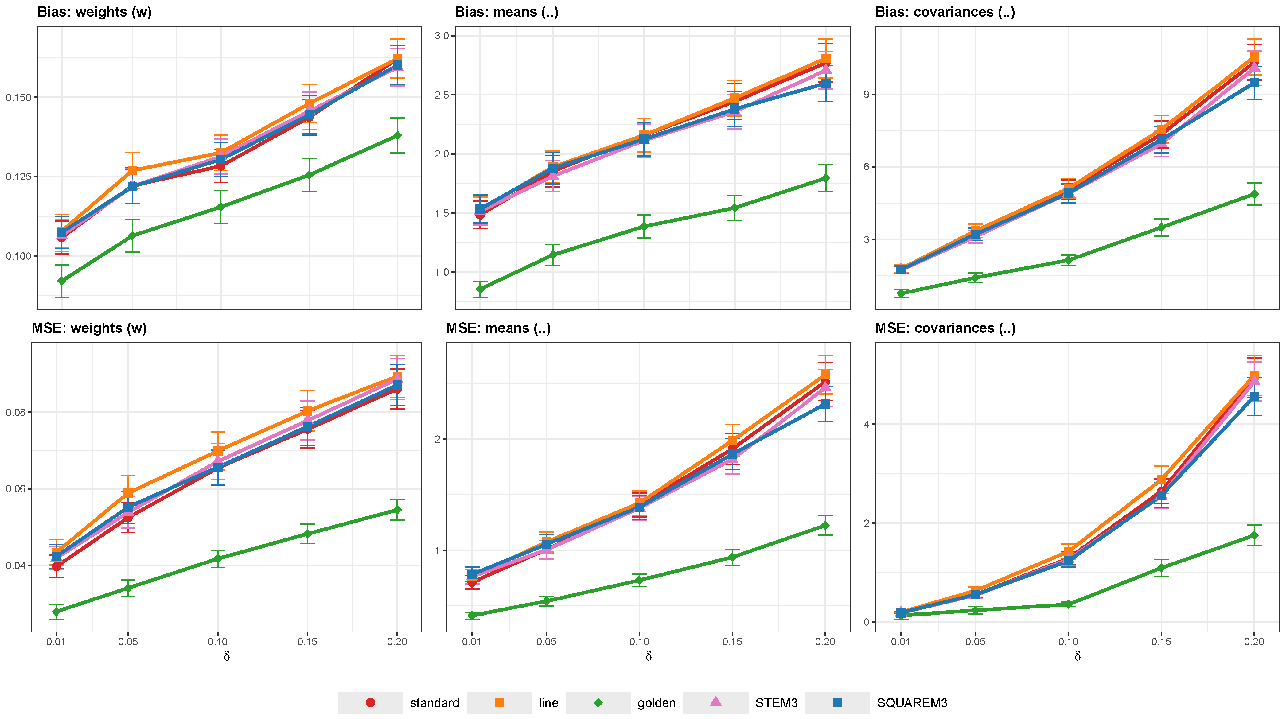
A central question is whether acceleration schemes that reduce iteration counts also degrade the quality of parameter estimates. Figure 2 presents the mean bias and mean squared error for weights, means, and covariance matrices as a function of overlap $\delta$, averaged across all sample sizes, dimensionalities, component counts, and initialisations. Values are clipped at the 99th percentile to prevent distortion from a small number of degenerate runs associated with the golden section scheme.

Standard EM, STEM, and SQUAREM produce virtually identical parameter estimates across all six metrics and all overlap levels. The lines overlap almost perfectly in every panel, confirming that acceleration with ${\alpha }_3$ does not introduce systematic bias or increase estimation variance. Line search yields marginally higher bias and MSE for means and covariances at high overlap, likely because its aggressive per-iteration optimisation occasionally overshoots into regions of the parameter space that are harder to recover from.

The golden section scheme presents a paradox: after clipping, it appears to produce the best estimates—lowest bias and MSE across all panels. However, this is a survivorship effect—that is, the clipping procedure preferentially removes the golden scheme’s degenerate runs, and the remaining sample is no longer representative of the method’s overall performance. The golden scheme generated degenerate solutions with near-singular covariance matrices in a small but non-negligible fraction of runs, producing MSE values exceeding ${10}^{10}$. After clipping these extreme values, the surviving runs are precisely those where the greedy search successfully located a superior optimum. The unclipped mean log-likelihood for golden (−50,650) is an order of magnitude worse than standard EM (−1952), confirming that its apparent superiority in Figure 2 does not generalise.

Table 5. Mean ARI and median log-likelihood by acceleration method and overlap level $\delta$. The ARI spread across methods is less than $0.024$ at every overlap level, confirming that acceleration does not affect solution quality.

Method	Metric	Overlap Level $\mathit{\delta }$
		0.01	0.05	0.10	0.15	0.20
Standard	ARI	0.804	0.636	0.496	0.397	0.320
	Med. $logL$	329.6	−405.9	−888.2	−1168.5	−1645.8
Line	ARI	0.799	0.630	0.492	0.395	0.317
	Med. $logL$	289.6	−405.9	−888.0	−1166.1	−1646.1
Golden	ARI	0.824	0.653	0.515	0.422	0.334
	Med. $logL$	288.8	−440.0	−893.2	−1317.9	−1755.2
STEM	ARI	0.801	0.635	0.495	0.396	0.319
	Med. $logL$	288.0	−405.9	−888.4	−1168.9	−1648.1
SQUAREM	ARI	0.801	0.634	0.495	0.397	0.319
	Med. $logL$	286.9	−405.9	−887.7	−1167.5	−1646.5

reports the mean ARI and median log-likelihood across overlap levels for each method. Median log-likelihood is used rather than the mean to mitigate the influence of golden degenerate runs. The ARI values are nearly indistinguishable: the total spread across all five methods is $0.024$, and the acceleration method explains less than $0.1\%$ of the total variance in ARI (${\eta }^2=0.001$). For comparison, overlap level and the number of components each explain over $30\%$ of ARI variance (${\eta }^2=0.37$ and ${\eta }^2=0.32$, respectively). This confirms that the choice of acceleration scheme has no practical impact on clustering quality—the dominant factors are the inherent difficulty of the mixture (overlap, number of components, dimensionality) and sample size, not the optimisation strategy.

In summary, STEM and SQUAREM with ${\alpha }_3$ provide a 24–$29\%$ reduction in iterations (Section 6.1) without any measurable degradation in parameter estimation quality, clustering performance, or model fit. Acceleration is, for practical purposes, a free improvement to the EM algorithm in the settings studied here.

6.3. Interaction Between Initialisation and Acceleration

We now examine whether the benefit of acceleration depends on the initialisation method, and whether acceleration degrades estimation quality for any particular initialisation. This section first analyses the four initialisation methods (hclust, k-means, random, and REBMIX averaged across all its configurations), and then provides a detailed breakdown of REBMIX preprocessing and mode-traversing options.

6.3.1. Acceleration Benefit Across Initialisations

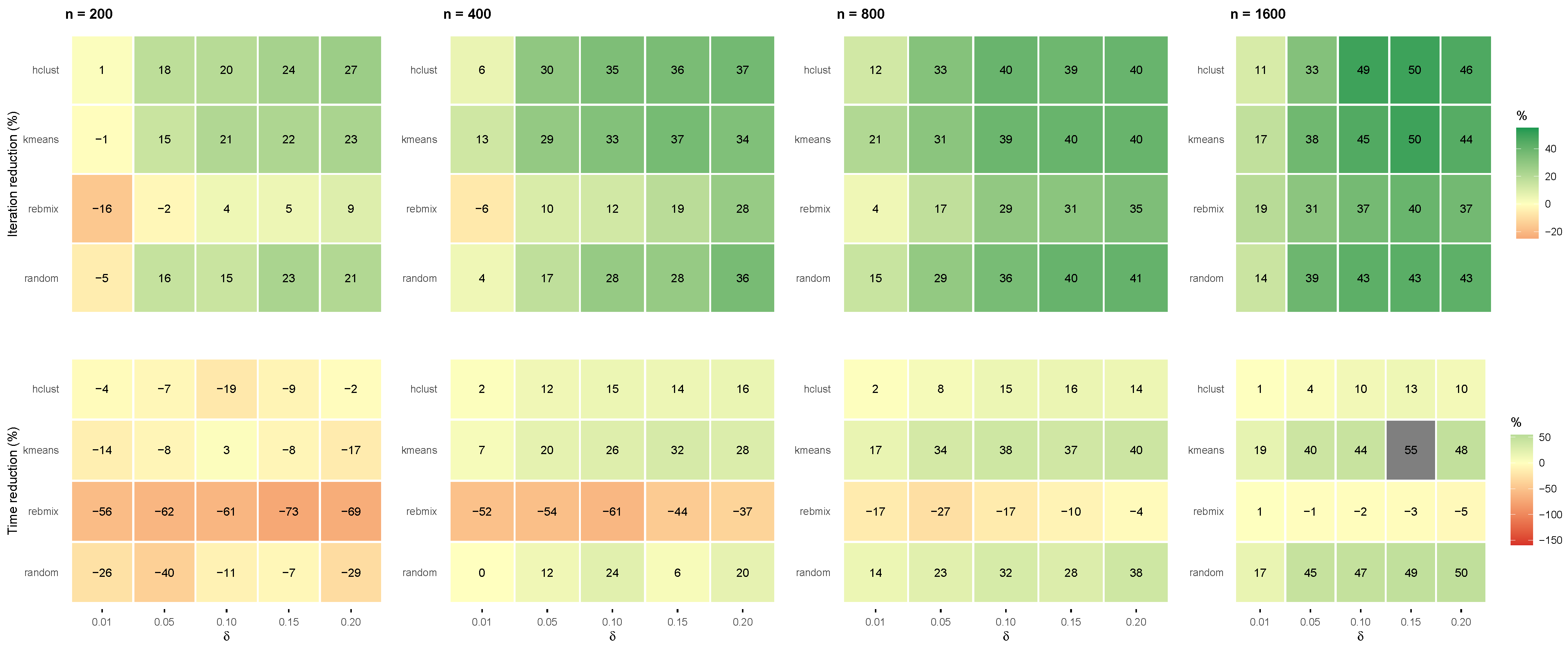
Figure 3 presents the average iteration reduction and time reduction achieved by STEM and SQUAREM (relative to standard EM) as a function of overlap $\delta$ and sample size n, separately for each initialisation method.

The benefit of acceleration varies substantially across initialisations. Hierarchical clustering and k-means benefit the most, with iteration reductions reaching 46–$50\%$ at $n=1600$ and $\delta \ge 0.1$. Random initialisation follows closely (43–$46\%$ at $n=1600$). REBMIX benefits the least, achieving only 35–$37\%$ at $n=1600$ and substantially less at smaller n. At $n=200$, REBMIX shows no iteration benefit (and slight degradation at low $\delta$), while hclust and k-means already achieve 15–$27\%$ reduction.

The time reduction (bottom row) reveals a more important distinction. For k-means and random, the iteration savings translate directly into wall-clock savings: up to 48–$50\%$ at $n=1600$. For hclust, the time savings are more modest (10–$13\%$ at $n=1600$) because the expensive $O\left(n^2\right)$ initialisation step dominates the total cost. For REBMIX, acceleration increases computation time at small n—by as much as $146\%$ at $n=200$—because the preprocessing step contributes substantially to the total cost, and the per-iteration overhead of computing ${\alpha }_3$ is not offset by the modest iteration savings. Only at $n\ge 1600$ does REBMIX begin to see marginal time savings.

This interaction has a practical implication: acceleration should always be applied when using k-means, random, or hclust initialisation, as the overhead is negligible and the potential savings are substantial. With REBMIX initialisation, acceleration is beneficial only at larger sample sizes ($n\ge 800$).

6.3.2. Estimation Quality Is Unaffected

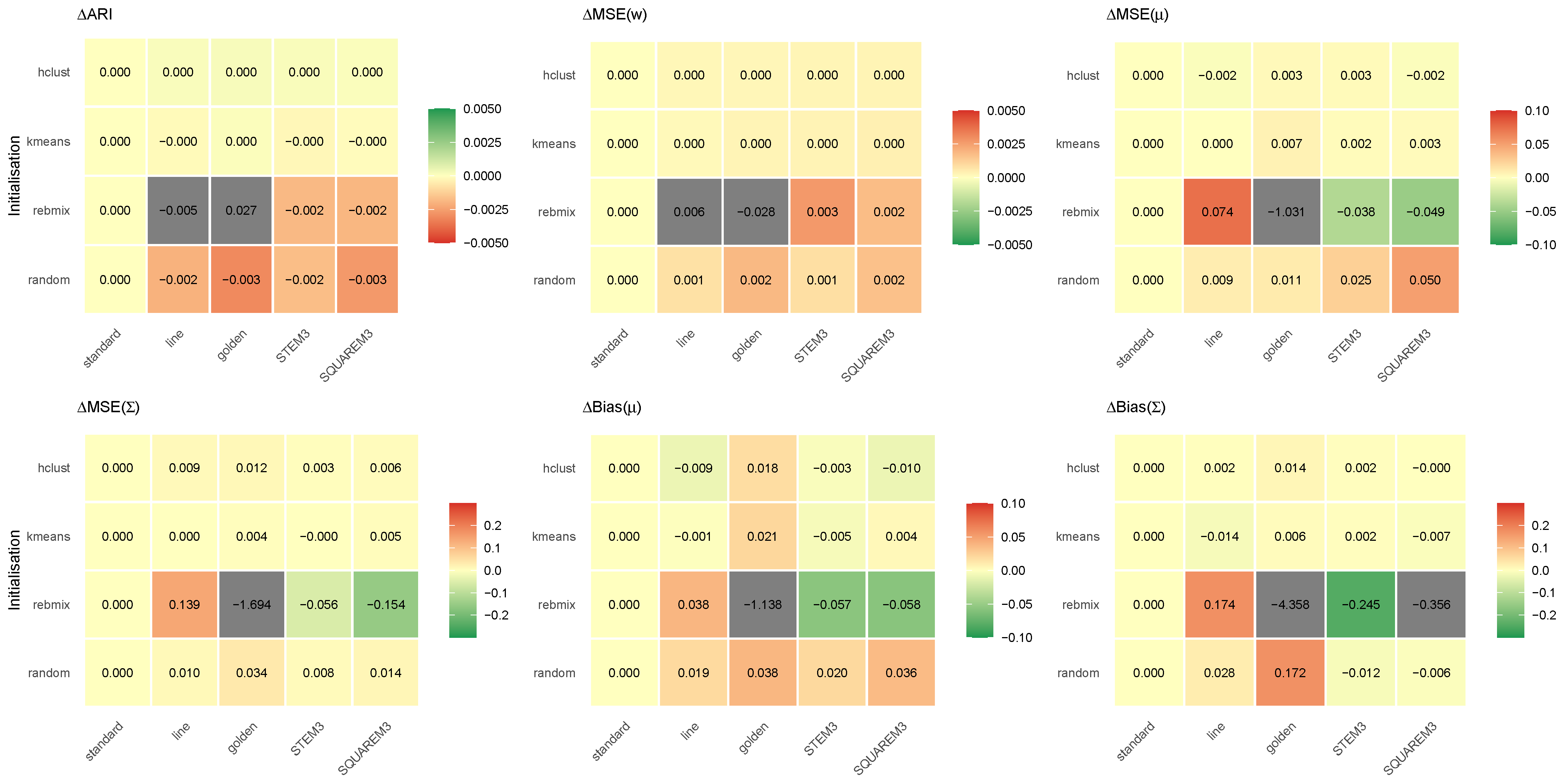
Figure 4 shows the change in six estimation quality metrics (ARI, MSE and bias for weights, means, and covariances) when switching from standard EM to each acceleration scheme, separately for each initialisation.

For hclust and k-means, all six quality metrics change by less than $0.004$ regardless of which acceleration scheme is used. The acceleration method ranking is also stable: the initialisation ranking (hclust > k-means > random > REBMIX by ARI) is preserved across all five acceleration schemes. Acceleration is therefore a quality-neutral transformation that can be applied independently of the initialisation choice.

For random initialisation, SQUAREM shows a small increase in MSE($\mathit{\mu }$) of $0.050$ and a small decrease in bias($\Sigma$) of $-0.402$, suggesting that the accelerated scheme occasionally converges to slightly different local optima when starting from a poor initialisation. These differences are small in practical terms and do not change the method ranking.

The golden section scheme shows anomalous behaviour with REBMIX: substantially lower MSE and bias values. As discussed in Section 6.2, this is a survivorship effect—the golden scheme’s degenerate runs are removed by clipping, and the surviving runs happen to reach superior optima.

6.3.3. REBMIX Configuration Analysis

The REBMIX algorithm offers three preprocessing methods and three mode traversing strategies. Figure 5 shows how the acceleration benefit varies across these nine configurations.

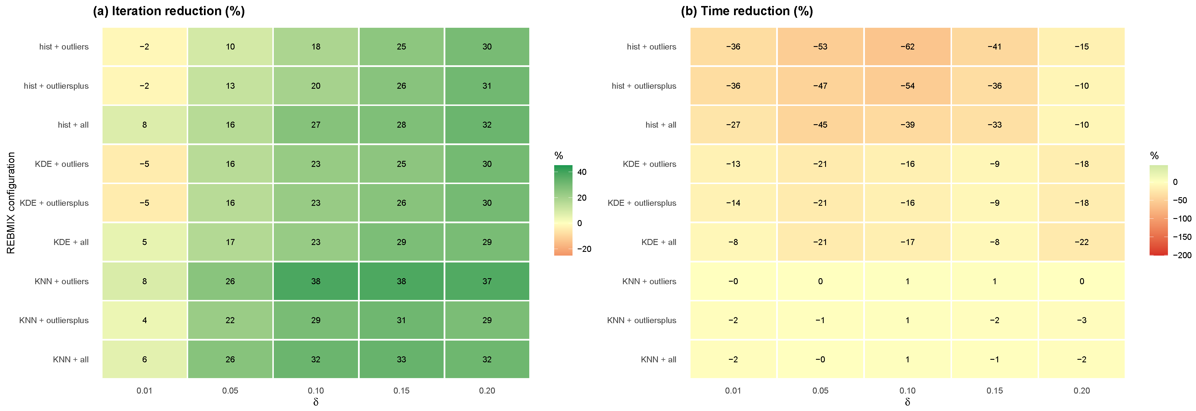
The iteration reduction pattern (Figure 5a) is consistent across preprocessing methods: all configurations show 15–$30\%$ reduction at high overlap, with the outliers mode benefiting slightly more than all or outliersplus. KNN with outliers shows the largest apparent reduction, but this reflects survivorship: this configuration completes only $37\%$ of the experimental grid, with failures concentrated at high d and high c where the EM problem is most difficult. When restricted to the same configurations where KNN succeeded, histogram preprocessing achieves equal or higher ARI.

The time reduction (Figure 5b) reveals the cost of preprocessing. Histogram configurations show the most favourable time profile (up to $20\%$ savings at high $\delta$), while KNN configurations show severe time penalties ($-100\%$ to $-200\%$, i.e., 2–$3\times$ slower) because the k-nearest neighbour preprocessing is $5\times$ more expensive than histogram binning, and this cost is not offset by the iteration savings.

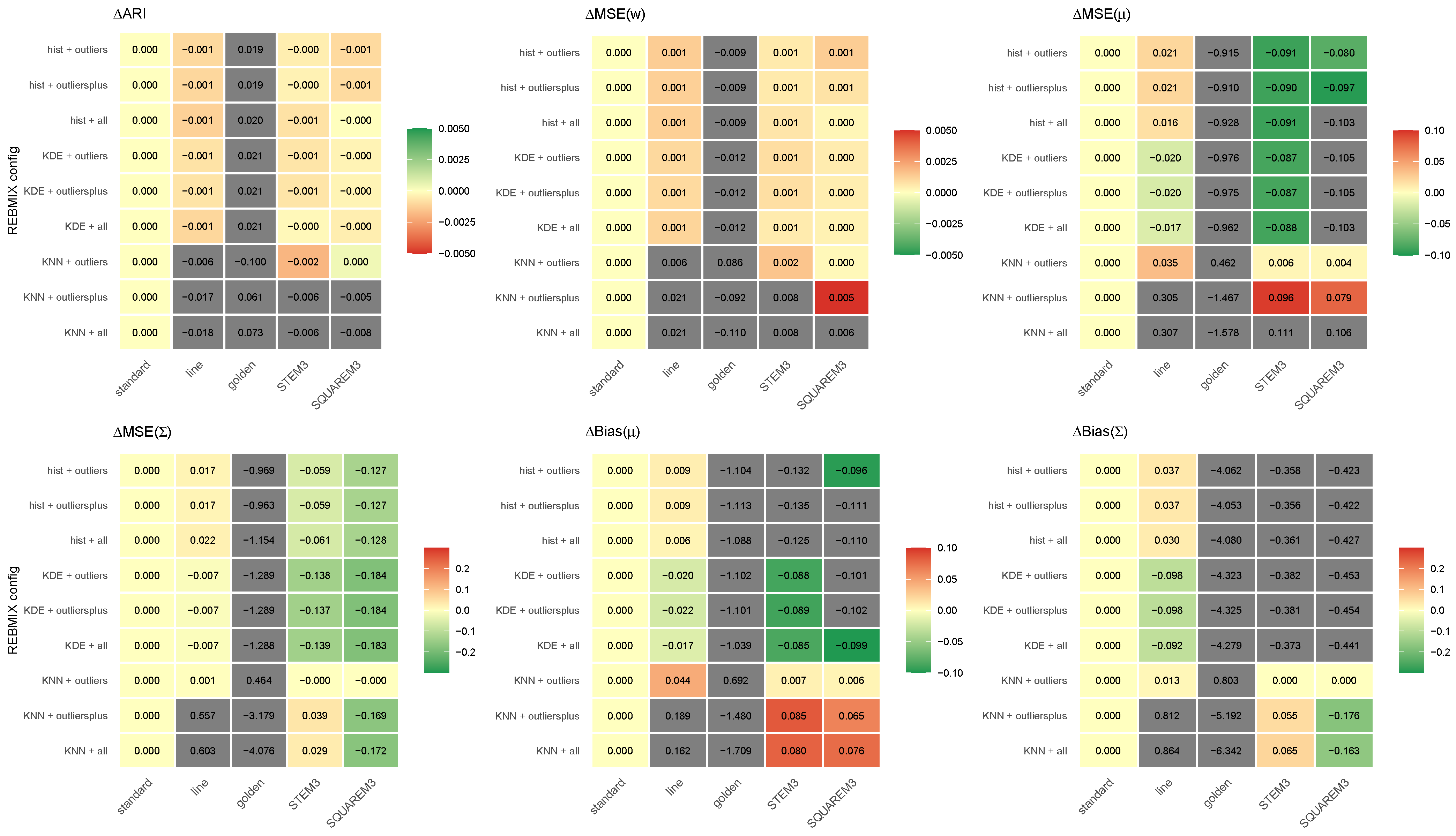
Figure 6 confirms that the choice of REBMIX configuration does not interact meaningfully with acceleration in terms of estimation quality: the $\Delta$MSE and $\Delta$bias values are negligible across all nine configurations and all acceleration schemes.

Based on these results, we recommend histogram preprocessing with the outliers mode traversing strategy as the default REBMIX configuration: it achieves the best ARI among configurations with full completion, requires the fewest iterations, and is the fastest. KDE is a viable alternative with equivalent quality but $1.5\times$ longer computation time. KNN preprocessing is not recommended due to its computational cost and poor scalability to high-dimensional, many-component settings.

7. Hard Drive Disk Failure Data Set

We analysed hard disk drive failure patterns using publicly available SMART telemetry data from Backblaze [28], covering drive failures from the years 2022, 2023, 2024, and Q1 of 2025. Each daily drive snapshot was filtered to retain only records associated with failed drives (failure > 0). This approach isolates the characteristics of drives at or near their point of failure, allowing for a more precise analysis of failure-related patterns. To ensure consistency across model types, all SSD models were excluded using a predefined list, focusing solely on mechanical hard drives, where mechanical wear and age-related degradation are dominant failure mechanisms.

The data set includes a total of 197 features, of which 186 correspond to SMART attributes, each reported in both raw and normalized form [29]. The remaining 11 features contain metadata such as date, serial number, model, capacity (in bytes), data center location (pod_id), and failure status. Normalized features are highly vendor-specific, and since the data set includes a variety of manufacturers, these features are not meaningful for comparison. In addition, many of the features are highly correlated, skewed, and sparse, often unreported or zero-valued across many models, which limits their usefulness in the context of mixture modelling.

We therefore selected only three SMART raw features: smart_9_raw (power-on hours), smart_193_raw (load cycle count), and smart_194_raw (temperature). These features account for most of the variance in the data and are also theoretically linked to reliability, as well as the mechanical and thermal load of the hard disk drive. The load cycle count exhibited low to moderate skewness and was log-transformed to mitigate this issue. All selected features were then rescaled to the $[0,1]$ interval after removing extreme outliers, defined as values outside the 2.5th to 97.5th percentile range, to ensure a uniform range across the data. Prior to rescaling, feature ranges varied considerably. Although the data set was not an ideal fit for Gaussian mixture modelling, this preprocessing enabled us to obtain reasonably interpretable results. After the final removal of missing values, the dataset contained 10,678 observations.

The number of mixture components was not known in advance. Except for different models of hard drive disks or possibly manufacturers, there was no other inherent labelling of the data that could be used as an initial guess. As there are over 50 different models, it is highly unrealistic that each represents a unique pattern. A second possible guess could be the number of hard drive manufacturers, which was five, namely HGST, Western Digital, Seagate, Toshiba, and Hitachi. Among these, only one hard disk drive model was from Hitachi; most of the hard disk drive models were Seagate drives, 5856 or 54.8%, the second largest group was Toshiba hard disk drive models, 2269 or 21.2%, followed by HGST hard disk drive models, 2079 or 19.4%, and a minority were Western Digital, 473 or 4.5%. Hence, there could be five, or more realistically four, major patterns, yet this is also highly unrealistic, as there may be other traits shared across different manufacturers. Therefore, we chose to use a model selection procedure and determine the best model via the Bayesian Information Criterion (BIC) [30],

$$\mathrm{BIC}=-2logL+Mlogn$$

(18)

where $logL$ is the obtained log-likelihood value, M is the number of parameters in the mixture model, and n is the number of observations. The minimum number of components was chosen as 2, and the maximum number of components was 10. We also used the same EM initialisations and acceleration schemes as in the simulation study.

Table 6. Results on the Backblaze hard drive dataset. Percentage reductions in iterations and time are relative to standard EM within each initialisation group. REBMIX configurations use outliersplus mode traversing.

Initialisation	Acceleration	Iterations		Time (s)		c	BIC
		Count	% Red.	Value	% Red.
k-means	Standard	2647	—	9.57	—	10	−19,496
	Line	1209	54.3	21.56	−125.3	10	−19,496
	Golden	1270	52.0	14.58	−52.4	10	−19,496
	STEM	1215	54.1	3.90	59.2	10	−19,496
	SQUAREM	1050	60.3	3.46	63.8	10	−19,496
Random	Standard	2549	—	8.25	—	9	−18,887
	Line	1593	37.5	26.75	−224.2	10	−19,428
	Golden	1762	30.9	18.61	−125.6	10	−19,428
	STEM	1455	42.9	4.28	48.1	10	−19,428
	SQUAREM	1062	58.3	3.53	57.2	9	−18,889
hclust	Standard	1922	—	159.43	—	10	−19,539
	Line	1022	46.8	169.78	−6.5	10	−19,539
	Golden	1070	44.3	164.24	−3.0	10	−19,539
	STEM	987	48.6	155.85	2.2	10	−19,539
	SQUAREM	960	50.1	155.66	2.4	10	−19,539
REBMIX (hist.)	Standard	666	—	1.85	—	10	−18,721
	Line	359	46.1	5.20	−181.1	10	−18,721
	Golden	370	44.4	3.37	−82.2	10	−18,721
	STEM	630	5.4	2.06	−11.4	10	−18,929
	SQUAREM	483	27.5	1.44	22.2	10	−18,929
REBMIX (KDE)	Standard	1736	—	8.43	—	10	−19,091
	Line	927	46.6	18.13	−115.1	10	−19,091
	Golden	964	44.5	13.04	−54.7	10	−19,091
	STEM	930	46.4	5.38	36.2	10	−19,091
	SQUAREM	819	52.8	5.02	40.5	10	−19,091
REBMIX (KNN)	Standard	1427	—	305.67	—	10	−18,752
	Line	1327	7.0	316.31	−3.5	10	−19,498
	Golden	1096	23.2	305.21	0.2	10	−19,361
	STEM	1317	7.7	298.43	2.4	10	−19,498
	SQUAREM	807	43.4	296.13	3.1	10	−18,770

presents the results for all six initialisation strategies. Most estimation strategies converge toward models with 10 components. The highest BIC value was achieved using hclust initialisation (−19,539), though at the cost of substantially longer processing time (155–170 s) due to the $O\left(n^2\right)$ agglomerative clustering step. The k-means initialisation yielded the second-highest BIC (−19,496) with reasonable computational time, and was therefore selected as the preferred method.

Across all estimation strategies, a consistent reduction in both computation time and the number of iterations was observed when using SQUAREM and STEM acceleration. SQUAREM achieved the largest iteration reductions (27–60%) and, with k-means initialisation, reduced computation time by $64\%$. As in the simulation study, line and golden section search effectively reduced the number of EM iterations but at the cost of increased computational time—line search was 2–$3\times$ slower than standard EM across all initialisations.

The interaction between initialisation and acceleration also confirms the simulation findings. With hclust, the $50\%$ iteration reduction translates to only $2\%$ time saving because the $O\left(n^2\right)$ initialisation dominates the total cost. With REBMIX histogram preprocessing, SQUAREM reduces iterations by $28\%$ and time by $22\%$—a more modest benefit than with k-means, consistent with the simulation observation that REBMIX starts closer to the optimum and thus benefits less from acceleration. REBMIX with KNN preprocessing is entirely dominated by the preprocessing cost (305 s), with acceleration contributing negligible time savings.

Notably, with random initialisation, standard EM and SQUAREM converge to a $c=9$ model (BIC = −18,887), while line search, golden section, and STEM find a $c=10$ model with substantially better BIC (−19,428). This suggests that the more exploratory search strategies occasionally escape local optima that trap the standard and quadratic acceleration schemes. However, this is an isolated observation; for all other initialisations, all acceleration schemes converge to the same solution, confirming the simulation finding that acceleration does not systematically alter the quality of the obtained estimates.

8. Conclusions

In this article, we have examined simple acceleration schemes applicable to the EM algorithm for Gaussian mixture modelling, with a focus on their behaviour under varying degrees of component overlap. We evaluated linear (STEM) and quadratic (SQUAREM) acceleration with three parameter estimates (${\alpha }_1$, ${\alpha }_2$, and ${\alpha }_3$), as well as greedy line search and golden section search, across a comprehensive simulation study comprising 240 mixture configurations (3 dimensionalities, 4 component counts, 5 overlap levels, and 4 sample sizes) and four initialisation methods (hierarchical clustering, k-means, random, and REBMIX). The findings were validated on a real-world Backblaze hard drive failure dataset.

A key empirical contribution of this study is the systematic comparison of the three acceleration parameter estimates proposed by [10]. Across all tested configurations, ${\alpha }_1$ and ${\alpha }_2$ consistently required more iterations than standard EM (52–$55\%$ and 35–$36\%$ more, respectively), effectively acting as deceleration. Only ${\alpha }_3$, the geometric mean of ${\alpha }_1$ and ${\alpha }_2$, provides genuine acceleration. This occurs because ${\alpha }_1$ and ${\alpha }_2$ frequently produce oversized step sizes that fail to increase the log-likelihood, triggering fallback to unaccelerated updates. This finding, which to our knowledge has not been documented for mixture modelling applications, confirms and strengthens the recommendation of [10] to use ${\alpha }_3$ exclusively.

With ${\alpha }_3$, both SQUAREM and STEM reduce EM iterations by $29\%$ and $24\%$ on average, with the benefit increasing monotonically with overlap level and sample size—reaching $48\%$ at $n=1600$ and $\delta =0.15$ for SQUAREM. The per-iteration overhead is minimal: at $n\ge 800$, the iteration savings translate directly into wall-clock time reductions. Line search and golden section search achieve larger iteration reductions (up to $40\%$) but increase total computation time by 50–$110\%$ due to repeated log-likelihood evaluations, making them impractical for routine use. The golden section scheme additionally exhibited catastrophic numerical instability in a small fraction of runs, producing degenerate covariance estimates.

Crucially, acceleration does not degrade estimation quality. Across all six metrics examined (ARI, log-likelihood, bias and MSE for weights, means, and covariances), the acceleration method explained less than $0.1\%$ of the total variance. The initialisation ranking was preserved regardless of which acceleration scheme was applied, confirming that the choice of acceleration and the choice of initialisation can be made independently.

The interaction between initialisation and acceleration revealed that REBMIX benefits least from acceleration ($20\%$ iteration reduction vs. 35–$37\%$ for other methods), because it already starts near the optimum. At small sample sizes, the per-iteration overhead of computing ${\alpha }_3$ can exceed the savings, making acceleration counterproductive for REBMIX at $n\le 400$. In contrast, k-means is the most favourable partner for acceleration, achieving up to $50\%$ time savings at $n=1600$. Among REBMIX configurations, the outliers mode traversing strategy consistently outperformed all and outliersplus, and histogram preprocessing offered the best cost-efficiency, being $1.5\times$ faster than kernel density estimation at equivalent quality and an order of magnitude faster than k-nearest neighbour preprocessing, which additionally failed to scale beyond $d=5$ or $c=5$.

The main findings of this study can be summarised as follows:

• Only the ${\alpha }_3$ estimate provides genuine acceleration; ${\alpha }_1$ and ${\alpha }_2$ act as deceleration and should not be used.
• SQUAREM with ${\alpha }_3$ is the most effective acceleration scheme, reducing iterations by up to $48\%$ with negligible per-iteration overhead.
• Acceleration effectiveness depends on sample size: benefits are negligible at $n\le 200$ and increase monotonically with n.
• Acceleration does not deteriorate parameter estimates under any tested combination of initialisation, dimensionality, number of components, or overlap level.
• Greedy methods (line search, golden section) reduce iteration counts but are computationally inefficient and, in the case of golden section, numerically unstable.
• Initialisation and acceleration do not interact: the initialisation ranking is preserved across all acceleration schemes, and acceleration benefits all initialisations (though REBMIX benefits least).
• For REBMIX, histogram preprocessing with outliers mode is recommended; k-nearest neighbour preprocessing is not recommended due to poor scalability.

In summary, practitioners fitting Gaussian mixture models should use SQUAREM with the ${\alpha }_3$ parameter estimate as their default acceleration scheme. The ${\alpha }_1$ and ${\alpha }_2$ estimates should be avoided entirely, as they reliably decelerate convergence. All methods evaluated in this study are implemented in the free and open-source R package rebmix, making acceleration readily available. For instance, enabling SQUAREM on the Backblaze hard drive dataset reduced computation time from $9.6$ s to $3.5$ s, which is a $64\%$ saving achieved by changing a single parameter in the estimation call. To our best knowledge, this capability is not natively available in any other R package for mixture modelling.

For future research, it would be valuable to investigate whether the acceleration behaviour observed here extends to non-Gaussian mixture models, constrained covariance structures (e.g., diagonal or tied covariances), and mixtures with very large numbers of components. Additionally, histogram-based EM schemes could substantially reduce per-iteration cost, potentially amplifying the benefits of acceleration in large-scale settings.

References

1. Dempster, A.P.; Laird, N.M.; Rubin, D.B. Maximum likelihood from Incomplete Data via the EM Algorithm. J. R. Stat. Soc. 1977, 39, 1–22. [Google Scholar] [CrossRef]
2. McLachlan, G.; Peel, D. Finite Mixture Models; John Wiley & Sons: New York, NY, USA, 2000. [Google Scholar]
3. Scrucca, L.; Karlis, D. A model-based approach to shot charts estimation in basketball. Comput. Stat. 2025, 40, 2031–2048. [Google Scholar] [CrossRef]
4. Fop, M.; Murphy, T.B.; Scrucca, L. Model-based clustering with sparse covariance matrices. Stat. Comput. 2019, 29, 791–819. [Google Scholar] [CrossRef]
5. Panić, B.; Nagode, M.; Klemenc, J.; Oman, S. On methods for merging mixture model components suitable for unsupervised image segmentation tasks. Mathematics 2022, 10, 4301. [Google Scholar] [CrossRef]
6. Xu, D.; Wang, Y. Density estimation for toroidal data using semiparametric mixtures. Stat. Comput. 2023, 33, 140. [Google Scholar] [CrossRef]
7. Cavicchia, C.; Vichi, M.; Zaccaria, G. Parsimonious ultrametric Gaussian mixture models. Stat. Comput. 2024, 34, 108. [Google Scholar] [CrossRef]
8. Novais, L.; Faria, S. Comparison of the EM, CEM and SEM algorithms in the estimation of finite mixtures of linear mixed models: A simulation study. Comput. Stat. 2021, 36, 2507–2533. [Google Scholar] [CrossRef]
9. Scrucca, L. Entropy-based anomaly detection for Gaussian mixture modeling. Algorithms 2023, 16, 195. [Google Scholar] [CrossRef]
10. Varadhan, R.; Roland, C. Simple and Globally Convergent Methods for Accelerating the Convergence of Any EM Algorithm. Scand. J. Stat. 2008, 35, 335–353. [Google Scholar] [CrossRef]
11. Baudry, J.P.; Celeux, G. EM for mixtures: Initialization requires special care. Stat. Comput. 2015, 25, 713–726. [Google Scholar] [CrossRef]
12. Scrucca, L.; Raftery, A. Improved initialisation of model-based clustering using Gaussian hierarchical partitions. Adv. Data Anal. Classif. 2015, 21, 3–8. [Google Scholar] [CrossRef] [PubMed]
13. Melnykov, V.; Melnykov, I. Initializing the EM algorithm in Gaussian mixture models with an unknown number of components. Comput. Stat. Data Anal. 2012, 56, 1381–1395. [Google Scholar] [CrossRef]
14. Panić, B.; Klemenc, J.; Nagode, M. Improved initialization of the em algorithm for mixture model parameter estimation. Mathematics 2020, 8, 373. [Google Scholar] [CrossRef]
15. You, J.; Li, Z.; Du, J. A new iterative initialization of EM algorithm for Gaussian mixture models. PLoS ONE 2023, 18, e0284114. [Google Scholar] [CrossRef]
16. Biernacki, C.; Celeux, G.; Govaert, G. Choosing starting values for the EM algorithm for getting the highest likelihood in multivariate Gaussian mixture models. Comput. Stat. Data Anal. 2003, 41, 561–575. [Google Scholar] [CrossRef]
17. Chassagnol, B.; Bichat, A.; Boudjeniba, C.; Wuillemin, P.H.; Guedj, M.; Gohel, D.; Nuel, G.; Becht, E. Gaussian Mixture Models in R. R J. 2023, 15, 56–76. [Google Scholar] [CrossRef]
18. Celeux, G.; Govaert, G. Gaussian parsimonious clustering models. Pattern Recognit. 1995, 28, 781–793. [Google Scholar] [CrossRef]
19. Beisemann, M.; Wartlick, O.; Doebler, P. Comparison of recent acceleration techniques for the EM algorithm in one-and two-parameter logistic IRT models. Psych 2020, 2, 209–252. [Google Scholar] [CrossRef]
20. Biernacki, C.; Celeux, G.; Govaert, G. Assessing a mixture model for clustering with the integrated completed likelihood. IEEE Trans. Pattern Anal. Mach. Intell. 2002, 22, 719–725. [Google Scholar] [CrossRef]
21. McNicholas, P.D.; Murphy, T.B.; McDaid, A.F.; Frost, D. Serial and parallel implementations of model-based clustering via parsimonious Gaussian mixture models. Comput. Stat. Data Anal. 2010, 54, 711–723. [Google Scholar] [CrossRef]
22. Saâdaoui, F. Acceleration of the EM algorithm via extrapolation methods: Review, comparison and new methods. Comput. Stat. Data Anal. 2010, 54, 750–766. [Google Scholar] [CrossRef]
23. Melnykov, V.; Chen, W.C.; Maitra, R. MixSim: An R Package for Simulating Data to Study Performance of Clustering Algorithms. J. Stat. Softw. 2012, 51, 1–25. [Google Scholar] [CrossRef]
24. Nagode, M. Finite mixture modeling via REBMIX. J. Algorithms Optim. 2015, 3, 14–28. [Google Scholar] [CrossRef]
25. Nagode, M.; Klemenc, J. Modelling of load spectra containing clusters of less probable load cycles. Int. J. Fatigue 2021, 143, 106006. [Google Scholar] [CrossRef]
26. Hubert, L.; Arabie, P. Comparing partitions. J. Classif. 1985, 2, 193–218. [Google Scholar] [CrossRef]
27. Kuhn, H.W. The Hungarian method for the assignment problem. Nav. Res. Logist. Q. 1955, 2, 83–97. [Google Scholar] [CrossRef]
28. Backblaze. Hard Drive Data and Stats. 2025. Available online: https://www.backblaze.com/cloud-storage/resources/hard-drive-test-data (accessed on 10 June 2025).
29. Coughlin, T.M. Chapter 2—Fundamentals of Hard Disk Drives. In Digital Storage in Consumer Electronics; Broy, M., Denert, E., Eds.; Newnes: Burlington, MA, USA, 2008; pp. 25–51. [Google Scholar]
30. Schwarz, G. Estimating the dimension of a model. Ann. Stat. 1978, 6, 461–464. [Google Scholar] [CrossRef]
Figure 1. Mean EM iterations (top) and computation time on a logarithmic scale (bottom) as a function of overlap δ , faceted by sample size n. Error bars indicate ±1 standard error. Three groups emerge: α 1 / α 2 variants (faint dotted/dashed) require more iterations than standard EM; line and golden search (dashed orange/green) achieve the fewest iterations but at substantially higher computation time; STEM and SQUAREM with α 3 (bold solid pink/blue) reduce both iterations and time relative to standard EM at moderate-to-high overlap.
Mathematics 14 01543 g001
Figure 2. Mean bias (top row) and mean squared error (bottom row) for weights, means, and covariance matrices as a function of overlap δ . Error bars indicate ±1 standard error. Values are clipped at the 99th percentile. Standard EM, STEM, and SQUAREM produce nearly identical estimates. Golden section search yields lower bias and MSE in the clipped data, but this reflects survivorship: its degenerate runs (MSE > 10 10 ) are removed by clipping.
Mathematics 14 01543 g002
Figure 3. Average STEM/SQUAREM iteration reduction (top) and time reduction (bottom) relative to standard EM, by initialisation, overlap δ , and sample size n. Green indicates improvement; red indicates degradation. Gray blocks are values above 99th percentile. REBMIX (averaged across all configurations) benefits least from acceleration, particularly in computation time.
Mathematics 14 01543 g003
Figure 4. Change in estimation quality relative to standard EM by initialisation and acceleration method. Values are clipped at the 99th percentile. Gray blocks are values above 99th percentile. For hclust, k-means, and random, all deltas are negligible (<0.005). The golden section scheme shows larger deviations due to survivorship bias from degenerate runs.
Mathematics 14 01543 g004
Figure 5. Average STEM/SQUAREM iteration reduction (a) and time reduction (b) for each REBMIX configuration. Histogram and KDE behave similarly; KNN with outliers mode shows the largest iteration reduction but is subject to survivorship bias (only 37 % completion rate).
Mathematics 14 01543 g005
Figure 6. Change in estimation quality relative to standard EM for each REBMIX configuration. All deltas are negligible, confirming that the preprocessing and mode traversing choices do not interact with the acceleration method. Gray blocks are values above 99th percentile.
Mathematics 14 01543 g006