Comparative Performance Analysis of Machine Learning Computational Pipelines and Deep Learning Architectures in EEG Motor Imagery BCIs

Abstract

The deployment of Motor Imagery Brain–Computer Interfaces (MI-BCI) is constrained by the inherent physiological variabilities of Electroencephalography (EEG) and parametric opacity. This paper presents a targeted technical audit of ten high-density MI-BCI computational pipelines, evaluating how existing literature addresses low Signal-to-Noise Ratio (SNR), intra-subject variability, and session-to-session instability. The investigation focuses on the contamination of data by ocular and muscular artifacts that overlap with the spectral components of Mu and Beta rhythms, often leading to algorithmic overfitting. Furthermore, the paper evaluates the impact of manifold drift where fluctuations in user state necessitate frequent recalibration as a primary hurdle for BCI portability. By applying a forensic evaluation framework to standardize the analysis across the ten selected studies, this paper identifies a high-performance landscape within standardized benchmarks, with classification accuracies reaching peak values of 95.42%. The audit specifically identifies a performance-reporting gap; while hybrid architectures demonstrate superior noise-rejection, they are frequently characterized by undocumented computational overhead. Additionally, while Neighborhood Component Analysis (NCA) emerges as a stable feature selection algorithm across the sampled literature, the systemic absence of reported execution times prevents a verified assessment of its low-latency viability. A critical technical finding is the widespread issue of Parametric Opacity, particularly regarding the omission of essential deterministic variables such as filter orders, windowing constants, and the final dimensionality of feature vectors. The audit reveals that the frequent failure to report the exact number of features utilized for classification masks potential overfitting and prevents an accurate assessment of the system’s generalization capabilities. Furthermore, only a specialized subset of the reviewed literature validates performance through formal statistical testing, such as Friedman ANOVA or Wilcoxon Signed-Rank tests, with most studies relying on peak accuracy metrics that may disguise filtered artifact residuals. This lack of granular documentation disguises the computational complexity of proposed methods and complicates their feasibility for hardware-in-the-loop validation. The findings establish that standardizing the reporting of preprocessing variables and feature-space dimensions is a prerequisite for overcoming current performance plateaus in universal BCI architectures.

1. Introduction

1.1. Biological Foundation

Brain–Computer Interface (BCI) technology creates a direct link between neural activity and external hardware, such as robotic prosthetics or wheelchairs. The system operates by decoding Motor Imagery (MI), which is the mental imagination of a physical action without any actual muscle movement [1,2]. This process allows an individual to produce control commands through endogenous brain signals. Electroencephalography (EEG) is the primary tool used to record these signals. It is popular in research because it is non-invasive, mobile, and possesses high temporal resolution [3,4]. EEG sensors track the brain’s electrical oscillations, which are divided into specific frequency bands based on the user’s state. The frequency bands are often referred to as brain waves, each associated with specific roles detailed in

Table 1. Frequency Bands of EEG Signal [5,6].

Frequency Band	Frequency Range	Amplitude (µV)	Properties
Delta	0.1–4 Hz	20–200	High Amplitude, slow wave. Slow wave found in deep sleep
Theta	4–8 Hz	10	Deep relaxation and meditation
Alpha	8–13 Hz	2–100	Daydream, calm state
Beta	13–30 Hz	5–10	Alert, active thinking, anxiety, panic attack, focus and concentration
Gamma	>30 Hz	-	Combination of two senses

. Arranged from lowest to highest frequency, scalp EEG captures five main categories: delta, theta, alpha, beta, and gamma. There is typically an inverse correlation between the frequency and amplitude of these physiological waveforms. Faster waves such as alpha and beta generally show smaller amplitudes, whereas slower waves such as delta and theta tend to exhibit larger amplitudes [5].

Detecting MI relies on tracking specific sensorimotor rhythms, mainly within the Alpha and Beta frequency ranges. When an individual imagines moving a limb, a localized decrease in the power of these frequencies occurs known as Event-Related Desynchronization (ERD). In contrast, once the mental task is completed, the power levels rise known as Event-Related Synchronization (ERS). The precise identification of these shifts in amplitude serves as the fundamental mechanism for converting mental intent into digital control commands [7]. Defining these frequency-dependent mechanisms is necessary to evaluate how various computational pipelines isolate and preserve the underlying physiological waveforms during feature extraction.

1.2. Artifacts and Noise

EEG signals are often contaminated by both physiological and non-physiological artifacts, which significantly lower the Signal-to-Noise Ratio (SNR). Artifacts are typically more stochastic than background EEG activity, exhibiting higher amplitudes and a transient, rather than rhythmic, nature. Three distinct sources of artifacts impact physiological recording sessions: environmental artifacts, experimental errors, and systemic physiological artifacts. Each of these sources possesses unique properties and manifests differently within the measured signal.

Environmental Artifacts: Environmental artifacts originate from the main power leads surrounding the body and typically appear as a 50/60 Hz hum. This interference can also stem from electromagnetic disturbances, where radiation emitted from external sources affects the recorded data. The measurement cables or the human body itself may act as an antenna, picking up radio frequency (RF) interference. Additionally, the recording leads can induce magnetic interference. They can generally be removed using simple filtering techniques because these artifacts often occupy a narrow frequency band or reside outside the frequency range of interest for brain signals [8,9,10].

Experimental Error: Experimental errors manifest as uncontrolled or unwanted variations within the experimental setup. For instance, subject motion can cause the physical position of an electrode on the scalp to shift, which alters the electrical coupling and results in signal distortion. Movement can change the volume conduction between the electrode and the signal source, inducing fluctuations in potential. These various factors result in the production of significant artifacts on the recorded output [8,9,10].

Physiological Artifacts: Systemic physiological artifacts are signal variations caused by biological processes other than neural activity. Among these, eye movements have the most detrimental effect on the EEG signal. The electrooculogram (EOG) measures the shift in the resting potential of the retina as the eye changes position. Blinking similarly triggers involuntary retinal movement and activates the eye muscles. Due to the proximity of the eyes to the brain, these signals propagate across the scalp and appear in the EEG as large-scale artifacts, often with amplitudes many times greater than the neural signals of interest. Muscle movements, or electromyography (EMG) artifacts, also impact recordings because they can originate from any muscle in the body and cover a broad frequency range. Specifically, tension in the facial and jaw muscles significantly distorts EEG data. Cardiac activity can introduce artifacts where the electrical output of the heart possesses high signal strength and can be detected at various positions on the body. This can lead to pulse artifacts, where the rhythmic expansion and contraction of blood vessels introduce voltage fluctuations into the recorded signal [8,9,10].

Table 2. Properties of Artifacts [6,11].

Artifact/Noise	Frequency Range	Amplitude/Propagation
Eye blink	<4 Hz	High amplitude (80–100 mV), low propagation
Eye Movement	<4 Hz	High Propagation
Forehead Movement	>13 Hz	High Amplitude
Electrode Displacement	<4 Hz	High Amplitude (20 mV)
Jaw clenching	>13 Hz	0–10 mV
Line Noise	50–60 Hz	Low Amplitude
Cardiac	>1 Hz	1–10 mV range
Muscle	≤35 Hz	Low amplitude (0–10 mV)

categorizes the primary sources of interference in EEG recordings based on their frequency characteristics and physical behavior. For a BCI system, understanding these ranges is critical because certain artifacts often overlap with the brain’s functional rhythms such as Alpha and Beta, making filtering a mathematical challenge.

These artifact properties establish the spectral boundaries required to assess whether reported filtering and denoising configurations are mathematically sufficient to isolate the neural signal of interest.

1.3. The Necessity for Machine Learning and Deep Learning

The integration of MI-BCI into assistive devices is frequently obstructed by three persistent technical hurdles: signal integrity (Low SNR), subject variability, and Parametric Opacity. First, a low Signal-to-Noise Ratio (SNR) of EEG requires frameworks robust enough to isolate brain activity from a dominant noise floor. However, many benchmarks rely on non-causal, zero-phase filtering that assumes a symmetric view of the signal, which is not reliable in a real-time MI-BCI. While [3,12,13] maximize accuracy by scaling feature vectors, a lack of transparency regarding causal filter coefficients and phase-response characteristics renders these benchmarks difficult to replicate in real-time. To counter low SNR, Refs [14,15] employ Deep Learning for spatial-temporal mapping, while [16,17] use Regularized CSP and Riemannian geometry to stabilize signals. Second, models face degradation due to inter-subject variability, session-to-session variation, and intra-subject non-stationarity. Spatial transformations optimized for specific cortical geometries often fail to generalize, leading to subspace over-fitting. To optimize the pipeline, Refs [7,18,19] use feature selection, yet these methods are often so precisely tuned to a single subject, that they lose generalizability across broader populations and separate recording sessions. Finally, Parametric Opacity remains a constraint, as studies often omit deterministic variables such as filter orders, cutoff frequencies, or regularization constants. This paper contributes a forensic technical audit designed to bridge the gap between reported performance and practical engineering suitability. Moving beyond a general survey, this work evaluates ten selected MI-BCI pipelines based on their causal reliability and the transparency of their governing parameters. By extracting exact numerical constants and identifying prevalent reporting deficits, this paper provides a concrete framework for developing reproducible BCI architectures. This audit serves as a necessary benchmark for transitioning theoretical research into functional applications. This consolidation is essential to identify which frameworks maintain the temporal integrity and generalizability necessary for reliable, sequential control in assistive technologies. To achieve this objective, this paper addresses the following research questions:

RQ1: How do the reviewed computational pipelines address the inherent challenges of low SNR and session-to-session variability in EEG signals?

RQ2: To what extent does the MI literature provide hyperparameters and parameters necessary for the replication of reported results or methods?

RQ3: Based on a forensic audit of 10 sampled studies, what are the most prevalent reporting gaps, and how do these constraints (documented as None Specified) hinder the transition of BCI research to functional, real-time environments?

To ensure mathematical clarity, a comprehensive summary of symbols and notation is provided in Appendix A 

Table A1. Summary of Mathematical Notations and Variable Definitions.

Variable	Definition	Domain/Section
$A_K$	Feedback Coefficients	Preprocessing
$B_K$	Feedforward Coefficients	Preprocessing
K	Filter order	Preprocessing
$y\left(n\right)$	Output signal	Preprocessing
x(n)	Input Signal	Preprocessing
h(K)	Impulse Response Coefficients	Preprocessing
N	Length of filter	Preprocessing
$y\left(t\right)$	Moving Average result	Preprocessing
t	time	Preprocessing
$x(t-i)$	Input signal at time (t − i)	Preprocessing
M	Number of samples	Preprocessing
x$\left(t\right)$	EEG signal	Artifact Removal—ICA
$\mathbf{s}\left(t\right)$	Independent source signals	Artifact Removal—ICA
${\mathbf{s}}_i\left(t\right)$	Independent components	Artifact Removal—ICA
$\mathbf{A}$	Mixing matrix	Artifact Removal—ICA
$c_1\left(t\right)$	difference in signal and curvature average	Decomposition—EMD
$h_1\left(t\right)$	Average of the two curvatures	Decomposition—EMD
$h_{11}\left(t\right)$	upper and lower average value of $c_1$.	Decomposition—EMD
$x_t$	EEG data segment	Artifact Removal—ASR
$M_r$	Mixing Matrix	Artifact Removal—ASR
$S_t$	Latent components	Artifact Removal—ASR
k	User-defined parameter	Artifact Removal—ASR
${\mu }_i$	Mean of RMS values	Artifact Removal—ASR
${\sigma }_i$	Standard Deviation of RMS values	Artifact Removal—ASR
$X_i$	Current channel matrix	Artifact removal—rASR
$n_{data}$	Number of samples	Artifact removal—rASR
c	Channels	Artifact removal—rASR
${\delta }_R$	geodesic Riemannian distance	Artifact removal—rASR
P(c)	c × c symmetric positive definite (SPD) matrices	Artifact removal—rASR
a(n)	AR parameters	Feature Extraction—AR
r	Model order	Feature Extraction—AR
e(n)	Prediction errors	Feature Extraction—AR
$N_{real}$	Sequence of real or complex numbers	Feature Extraction—FFT
X(k)	Frequency components	Feature Extraction—FFT
$\phi$	Mother Wavelet	Feature Extraction—WT
a	Scale parameter	Feature Extraction—WT
$\mathsf{\tau }$	Shift Parameter	Feature Extraction—WT
$\vartheta \left(x\right)$	Scaling function	Feature Extraction—WT
$\phi \left(x\right)$	Wavelet function	Feature Extraction—WT
$M_p$	Power of 2	Feature Extraction—WT
$f_s$	Sampling Frequency	Feature Extraction—WT
l	Level of decomposition	Feature Extraction—WT
${\overline{R}}_1$ and ${\overline{R}}_2$	Averaged class-specific covariance matrix	Feature Extraction—CSP
R	Composite covariance matrix	Feature Extraction—CSP
$U_0$	eigenvectors	Feature Extraction—CSP
$\sum$	Diagonal Matrix of corresponding eigenvalues	Feature Extraction—CSP
P	Whitening transformation matrix	Feature Extraction—CSP
$W_{spatial}$	Spatially filtered Signal	Feature Extraction—CSP
$x_i$	Sample data	Feature Extraction—PCA
$C_x$	Covariance matrix	Feature Extraction—PCA
$v_m$	Eigenvectors	Feature Extraction—PCA
${\lambda }_m$	Eigenvalues	Feature Extraction—PCA
$w_{ji}$	Predictor weight	Feature Selection—Relief-f
${\Delta }_j(x_G,x_H)$	Absolute difference between the jth feature of $x_G$ and $x_H$	Feature Selection—Relief-f
$p_{yH}$	Prior probability of the class y associated with instance H	Feature Selection—Relief-f
$p_{yG}$	Prior probability of the class y associated with instance G	Feature Selection—Relief-f
$M_{iter}$	Number of iterations	Feature Selection—Relief-f
$d_{GH}$	Scaled distance between $x_G$ and $x_H$	Feature Selection—Relief-f
${\mathit{A}}_{\mathit{a}\mathit{d}\mathit{j}}$	Adjacency Matrix	Feature Selection—ILFS
$\lambda$	Loading coefficient	Feature Selection—ILFS
$E_p$	Energy of feature subset	Feature Selection—ILFS
I	Identity Matrix	Feature Selection—ILFS
e	1D array of ones	Feature Selection—ILFS
$r$	Real-valued regularization factor:	Feature Selection—ILFS
$n_{nodes}$	Number of nodes	Feature Selection—ILFS
L	Path length	Feature Selection—ILFS
$\left|I_{set{1}^{\prime }}\left(x\right)\right|$ and $\left|I_{set{2}^{\prime }}\left(x\right)\right|$	First derivatives of the datasets regarding x,	Feature Selection—FSV
$x_{max}$ and $x_{min}$	Range of x values	Feature Selection—FSV
c	Ratio of the average intensities of the datasets	Feature Selection—FSV
$GD{M}_i$	GDM index	Feature Selection—FSV
$AD{M}_i$	ADM index	Feature Selection—FSV
$FD{M}_i$	FDM index	Feature Selection—FSV
Y	Quantized feature values	Feature Selection—SD
p(y, z)	Joint occurrence frequency of a feature value and a class label	Feature Selection—SD
p(y) and p(z)	Probabilities of feature values and class labels.	Feature Selection—SD
$w_{l_f}$	Weight	Feature Selection—NCA
${\tau }_k$	Kernel function	Feature Selection—NCA
$\alpha$	Input parameter	Feature Selection—NCA
$\delta \left(w\right)$	Approximate LOO classification accuracy	Feature Selection—NCA
$N_{candidate}$	Number of candidate points	Feature Selection—NCA
$n_f$	Number of features	Feature Selection—mRMR
$\sum I(z,f)$	Mutual information between class label and features	Feature Selection—mRMR
$\sum I(f_1,f_2)$	Mutual information between two features	Feature Selection—mRMR

.

2. Materials and Methods

2.1. Literature Survey

The research was initiated through a chronologically unconstrained search for MI literature, prioritizing studies containing algorithmic derivations and governing equations. To ensure the retrieval of foundational source parameters, the search was conducted across four primary databases: Google Scholar, IEEE Xplore, PubMed, and Academia.edu. To secure a mathematically diverse representation of contemporary peer-reviewed studies, the identification process utilized:

• Specialized Discovery Tools: The search leveraged Anara to identify high-density technical papers and targeted MDPI journals for recent algorithmic contributions.
• Secondary Identification: To uncover latent information often obscured in primary studies, the process was reinforced by backward citation tracking and a selection of existing systematic reviews.
• Search Parameters: Searches were centered on the stages in a BCI pipeline: (“Motor Imagery” AND “EEG” AND “Review”), (“BSS” AND (“ASR” OR “ICA” OR “EMD”) AND “Motor Imagery”), (“Feature Selection” AND “Motor Imagery”), (“Feature Extraction” AND (“FFT” OR “DWT” OR “AR”)), (“Feature Extraction” AND “CSP” AND “PCA”), (“Classification” AND “Review” AND “Motor Imagery”), and (“Deep Learning” AND “Review” AND “Motor Imagery”).

2.1.1. Inclusion and Exclusion Criteria

A study was included in the final synthesis if it met the following four technical requirements:

Domain Relevance: The primary focus must be MI EEG signal classification.

Architectural Disclosure: The study must outline a partial/full processing pipeline, defining the transition from signal acquisition to classification.

Gradient of Parametric Transparency: This paper prioritizes the depth of technical disclosure over a high volume of studies. To facilitate a meaningful mathematical audit, a representative spectrum of literature was selected based on the clarity of reporting, ranging from papers providing full governing equations to those with None Specified parameters. This inclusion allows for an investigation into how missing details, such as specific filter orders, affect the overall reliability and reproducibility of BCI performance.

To ensure the accuracy of the mathematical audit and the integrity of the data extraction, the following exclusion criteria were applied:

Non-English Publications: Studies published in languages other than English were excluded to avoid technical translation errors.

Abstract-Only or Summary Reports: Short-form publications, such as posters or conference abstracts, which lacked the necessary space to disclose a full or partial processing pipeline.

Insufficient Parametric Resolution: Studies were excluded if the methodology was purely descriptive without providing the technical resolution required for a parametric audit. For example, a study stating ‘data was filtered’ without specifying the filter type, frequency cut-offs, or implementation stage provides a methodology, but lacks the architectural transparency required for this audit.

2.1.2. Screening Process

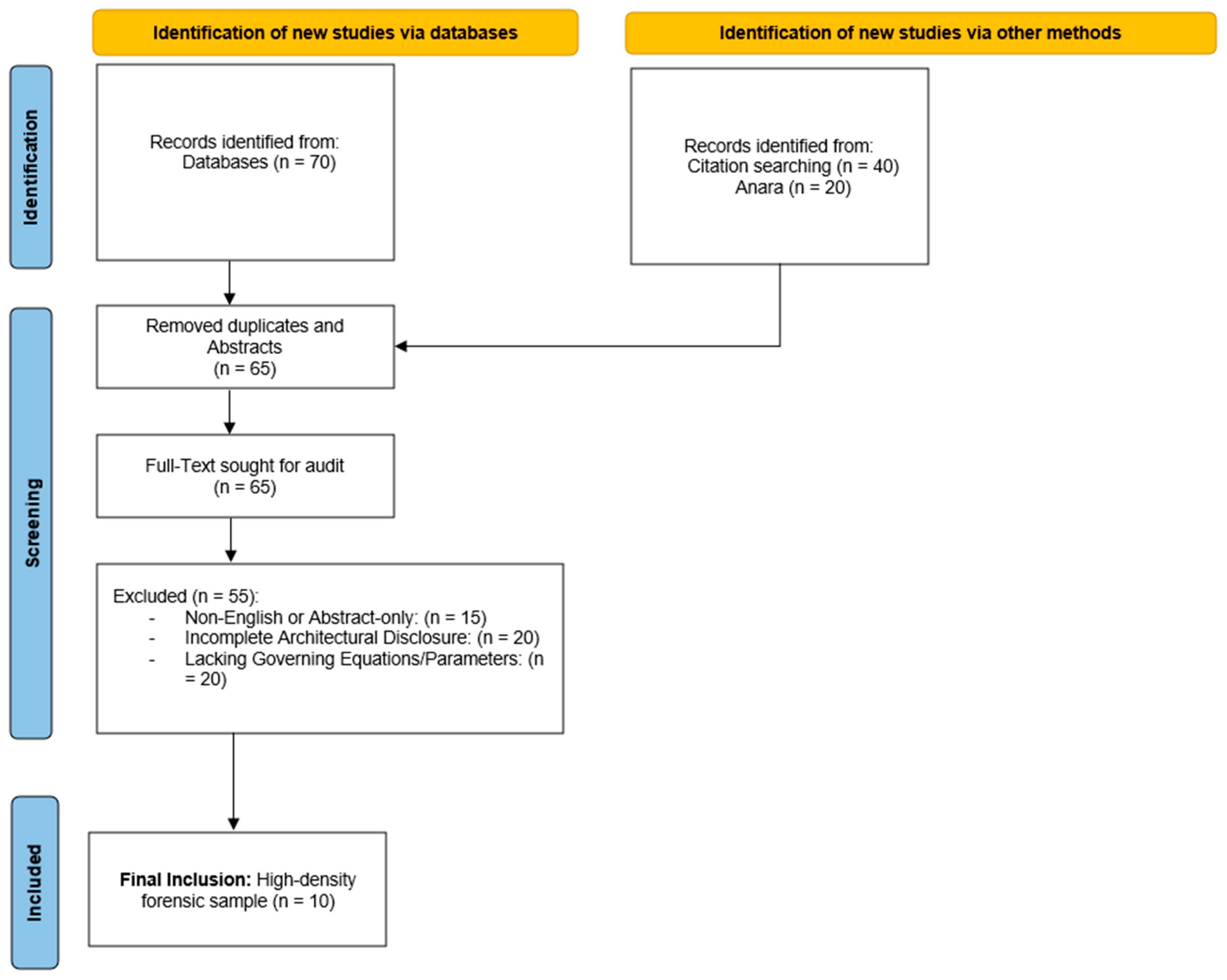
The selection process followed a structured screening funnel, shown in Figure 1, to transition from broad literature to a targeted forensic sample. An initial search from December 2025 for MI-BCI systems across major databases yielded an initial pool of 130 records. Following the removal of duplicates, studies were screened against the strict exclusion of non-English publications and short-form abstracts to ensure linguistic accuracy and sufficient technical depth for auditing. The remaining 65 articles underwent a full-text eligibility review based on the primary inclusion criteria: the presence of a traceable processing pipeline and governing equations. This thorough filtering resulted in a final synthesis of 10 high-density studies (

Table 3. Summary of Reviewed Studies including Dataset Origin, Subject Demographics, and Hardware Acquisition Parameters.

Paper	Year	Dataset Name	Subjects	Sampling Frequency	Electrodes	Filtering	Limitation
[12]	2015	Self-Generated	5	256 Hz	C3, C4, Cz (10–20 system)	-	Only five subjects (mean age 25.6 ± 2.3 yr) were tested, which limits statistical power and generalizability.
[16]	2019	Self-Generated	27	250 Hz	10–20 system	-	Evaluated rASR only on eye-blink artifacts and overlooked other physiological and non-physiological sources.
[3]	2020	BCI Comp III 4A BCI Comp IV 2B	5 9	1000 Hz 250 Hz	118 C3, C4, Cz	Bandpass—0.05–200 Hz Downsampled at 100 Hz Bandpass—0.5–100 Hz	Fixed trial windows ignore subject-specific latencies and transient signal dynamics.
[13]	2021	Physionet	109	128 Hz	64 (10–10 system)	-	Basic filters fail to achieve ideal noise removal, requiring complex hybrid processing for accuracy
[14]	2022	Self-Generated	57	250 Hz	16	Notch—32–48 Hz Bandpass—0.5–30 Hz	Did not assess subject-independent or multi-class scenarios
[15]	2023	BCI Comp IV 2A BCI Comp IV 2B Lab Data	9 9	250 Hz 250 Hz	25 C3, C4, Cz	Bandpass—0.5–100 Hz Notch—50 Hz Bandpass—0.5–100 Hz	Limited to Binary class imagery
[19]	2023	BCI Comp III 4A BCI Comp III 3B	5 9	1000 Hz 250 Hz	118 C3, C4, Cz	Bandpass—0.05–200 Hz Downsampled at 100 Hz Bandpass—0.5–100 Hz	Large-scale electrode setups create noisy, redundant data that degrades classification performance
[7]	2023	BCI Comp IV 1 BCI Comp III 4A	7 5	100 Hz 1000 Hz	59 118	- Bandpass—0.05–200 Hz Downsampled at 100 Hz	Framework targets binary motor-imagery EEG classification; multiclass extensions are suggested only for future work
[17]	2024	Self-Generated	5	None Specified	None Specified	-	Only five subjects were tested, which limits statistical power and generalizability
[18]	2024	BCI Comp III 4A BCI Comp III 3B BCI Comp III 3A	5 3 3	1000 Hz 125 Hz 250 Hz	118 C3, C4, Cz 64	Bandpass—0.05–200 Hz Downsampled at 100 Hz Notch—0.5–30 Hz Filter not specified but used a range of 1–50 Hz	Requires further real-world testing across different recording conditions and user demographics

). This sample size was intentionally constrained to 10 to facilitate a high-resolution audit. It was prioritized over a high-volume survey to ensure the identification of parameter gaps remained the focal point of the analysis. This approach prevents the core technical findings from being diluted in a larger, less transparent literature pool.

2.2. Data Acquisition

The process of recording EEG signals for MI is the foundation of a BCI system, as it determines the quality of the data before any processing begins. To ensure the results are consistent and can be repeated by other researchers, specific standards are followed regarding where the electrodes are placed, how fast the data is sampled, and how well the sensors connect to the scalp.

2.2.1. The International 10–20 System

The International 10–20 System serves as the universal standard for positioning electrodes during EEG recording. This method relies on the distance between specific anatomical landmarks, namely the Nasion (the bridge of the nose) and the Inion (the protrusion at the base of the skull), to define electrode sites. The terms “10” and “20” represent the specific intervals between adjacent electrodes, which are spaced at either 10% or 20% of the total longitudinal or transverse distance of the cranium [20].

In the context of MI, research typically emphasizes the Central (C) electrodes, as shown in

Table 4. Cortex and Electrode Regions [5,21].

Cortex Region	Function	Electrode
Frontal	Reasoning, speech, emotions, problem solving	F
Central	Sensorimotor (movement)	C
Parietal	Attention, processing of stimuli related to senses	P
Occipital	Vision	O
Temporal	Memory, auditory, stimuli interpretation and processing	T

, specifically C3, C4, and Cz as these positions correspond to the sensorimotor cortex. C3 represents the left hemisphere, C4 the right hemisphere, and Cz the midline. Following this standardized system is essential for the reliability of a review, as it ensures that specific electrode labels refer to the same cortical regions across different studies, allowing for a direct comparison of results [20].

2.2.2. Sampling Rate and Nyquist Criterion

Following the capture of microvolt-scale signals by the electrodes, the Data Acquisition system converts these analog potentials into digital samples. This process is dictated by the Nyquist-Shannon Sampling Theorem, which states that the sampling rate must be at least twice the highest frequency present in the signal to prevent aliasing, or digital distortion [20].

In the context of MI, the primary rhythms of interest, specifically the Mu and Beta bands reside within a relatively low frequency range. As a result, sampling rates between 250 Hz or 500 Hz are common throughout the literature. These rates provide a sufficient margin to capture the relevant brain dynamics while maintaining a manageable data throughput for digital filtering and real-time processing [20].

2.2.3. Electrode Type

The physical interface between the scalp and the electrode is a direct factor in the quality of the acquired data. Beyond spatial positioning, researchers must evaluate various electrode chemistries and electronic configurations, balancing the need for signal stability against the practicalities of setup speed and user comfort [22].

Wet versus Dry Electrodes: Traditional wet electrodes (Silver/Silver Chloride or Ag/AgCl) use a conductive gel or saline solution to maintain low skin-to-electrode impedance. This approach typically provides the highest signal fidelity and is widely considered the benchmark for recordings. In contrast, dry electrodes use mechanical pins or conductive fabrics to establish contact without the need for gel. While dry systems offer significantly faster setup times, they are generally more susceptible to the motion artifacts and signal instability discussed in Section 1.2 [22].

Active versus Passive Configurations: The electronic architecture of the sensor also impacts signal integrity. Passive electrodes act as a direct relay for the neural signal, which leaves the data vulnerable to environmental noise and cable sway interference. Active electrodes address it by implementing a pre-amplifier directly at the sensor site. This local amplification strengthens the signal before it travels through the cabling, significantly reducing electromagnetic interference. Such a configuration is particularly beneficial for maintaining a high Signal-to-Noise Ratio (SNR) in the environments required for real-time MI applications [22].

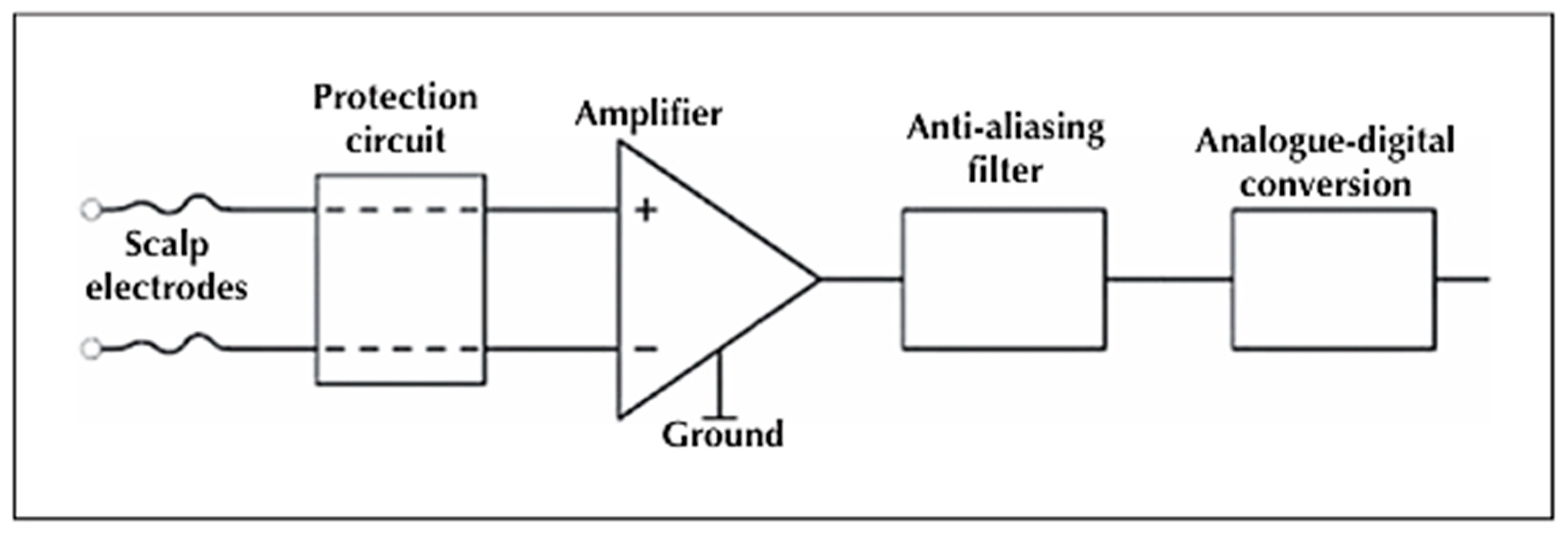
The acquisition stage shown in Figure 2 functions as a deterministic interface designed to isolate cortical oscillations from dominant extracerebral noise. The process initiates with a protection and isolation circuit, establishing a unidirectional electrical barrier for subject safety. Following stabilization, signals enter a differential amplifier to calculate the potential difference between active scalp electrodes and a Common Recording Reference (CRR). This configuration is mathematically justified by the volume conduction properties of the human body. High-amplitude artifacts such as cardiac pulses and myogenic contractions appear as common-mode signals across the scalp. By performing hardware-level subtraction the system suppresses these global interference patterns, effectively isolating low-voltage neural potentials from the environmental noise floor [20].

Figure 2. Standard signal acquisition chain in passive configuration. The schematic illustrates the hardware sequence from analog scalp interface to ADC quantization as identified in the reviewed literature. These stages establish the fundamental signal integrity and temporal resolution required for the digital preprocessing documented in Table 5 [20].

Figure 2. Standard signal acquisition chain in passive configuration. The schematic illustrates the hardware sequence from analog scalp interface to ADC quantization as identified in the reviewed literature. These stages establish the fundamental signal integrity and temporal resolution required for the digital preprocessing documented in Table 5 [20].

Table 5. Technical Specifications of Filtering and Windowing Techniques across Reviewed Literature.

Paper	Year	Filter Type	Filter Order	Frequency	Notes
[12]	2015	None Specified	None Specified	None Specified	Absence of filters leaves the system vulnerable to artifact contamination
[16]	2019	Low Pass High Pass	166 3300	40 Hz 0.25 Hz	High filter orders suggest high computational latency, potentially unsuitable for real-time BCI.
[3]	2020	Butterworth zero-phase bandpass	None Specified	8–35 Hz	Zero-phase filtering is non-causal; requires whole-buffer processing which limits online application.
[13]	2021	Two-pass forward and reverse zero phase non causal bandpass	None Specified	1–16 Hz	Eliminates phase distortion but introduces a non-causal operational boundary, making it unsuitable for real-time BCI.
[14]	2022	Butterworth Bandpass	5	7–30 Hz	Uses a lower-order filter to balance signal attenuation with processing speed.
[15]	2023	Butterworth Bandpass	6	0.5–40 Hz	Mid-range order optimized for spectral roll-off without excessive phase distortion.
[19]	2023	Bandpass	None Specified	8–35 Hz	Does not specify the filter order, creating a barrier for algorithmic benchmarking.
[7]	2023	Butterworth Bandpass	None Specified	8–15 Hz	Narrow band (8–15 Hz) limits the analysis to the Mu-rhythm, potentially ignoring valuable Beta-band features.
[17]	2024	Bandpass	None Specified	1–40 Hz	lack of order specification suggests the frequency roll-off characteristics ambiguous.
[18]	2024	Bandpass	None Specified	8–30 Hz	Uses a broad band (8–30 Hz) but omits the filter order for the digital implementation.

Table 5. Technical Specifications of Filtering and Windowing Techniques across Reviewed Literature.

Paper	Year	Filter Type	Filter Order	Frequency	Notes
[12]	2015	None Specified	None Specified	None Specified	Absence of filters leaves the system vulnerable to artifact contamination
[16]	2019	Low Pass High Pass	166 3300	40 Hz 0.25 Hz	High filter orders suggest high computational latency, potentially unsuitable for real-time BCI.
[3]	2020	Butterworth zero-phase bandpass	None Specified	8–35 Hz	Zero-phase filtering is non-causal; requires whole-buffer processing which limits online application.
[13]	2021	Two-pass forward and reverse zero phase non causal bandpass	None Specified	1–16 Hz	Eliminates phase distortion but introduces a non-causal operational boundary, making it unsuitable for real-time BCI.
[14]	2022	Butterworth Bandpass	5	7–30 Hz	Uses a lower-order filter to balance signal attenuation with processing speed.
[15]	2023	Butterworth Bandpass	6	0.5–40 Hz	Mid-range order optimized for spectral roll-off without excessive phase distortion.
[19]	2023	Bandpass	None Specified	8–35 Hz	Does not specify the filter order, creating a barrier for algorithmic benchmarking.
[7]	2023	Butterworth Bandpass	None Specified	8–15 Hz	Narrow band (8–15 Hz) limits the analysis to the Mu-rhythm, potentially ignoring valuable Beta-band features.
[17]	2024	Bandpass	None Specified	1–40 Hz	lack of order specification suggests the frequency roll-off characteristics ambiguous.
[18]	2024	Bandpass	None Specified	8–30 Hz	Uses a broad band (8–30 Hz) but omits the filter order for the digital implementation.

To ensure signal integrity for digital processing, the amplified analog potentials are subjected to anti-aliasing filtration. This stage permanently attenuates high-frequency components, such as the electromagnetic interference and EMG, which exceed the system’s operational Nyquist limit. This filtration is a prerequisite for accurate digitization as per the Nyquist-Shannon sampling theorem. Failing to suppress frequencies exceeding half the sampling rate would result in high-frequency noise folding into the Mu and Beta bands. This preventive measure eliminates permanent aliasing artifacts, establishing a conditioned, discrete data stream as the foundation for the subsequent BCI pipeline [20].

2.3. Real-Time and Dataset Description

2.3.1. Real—Time Acquisitions

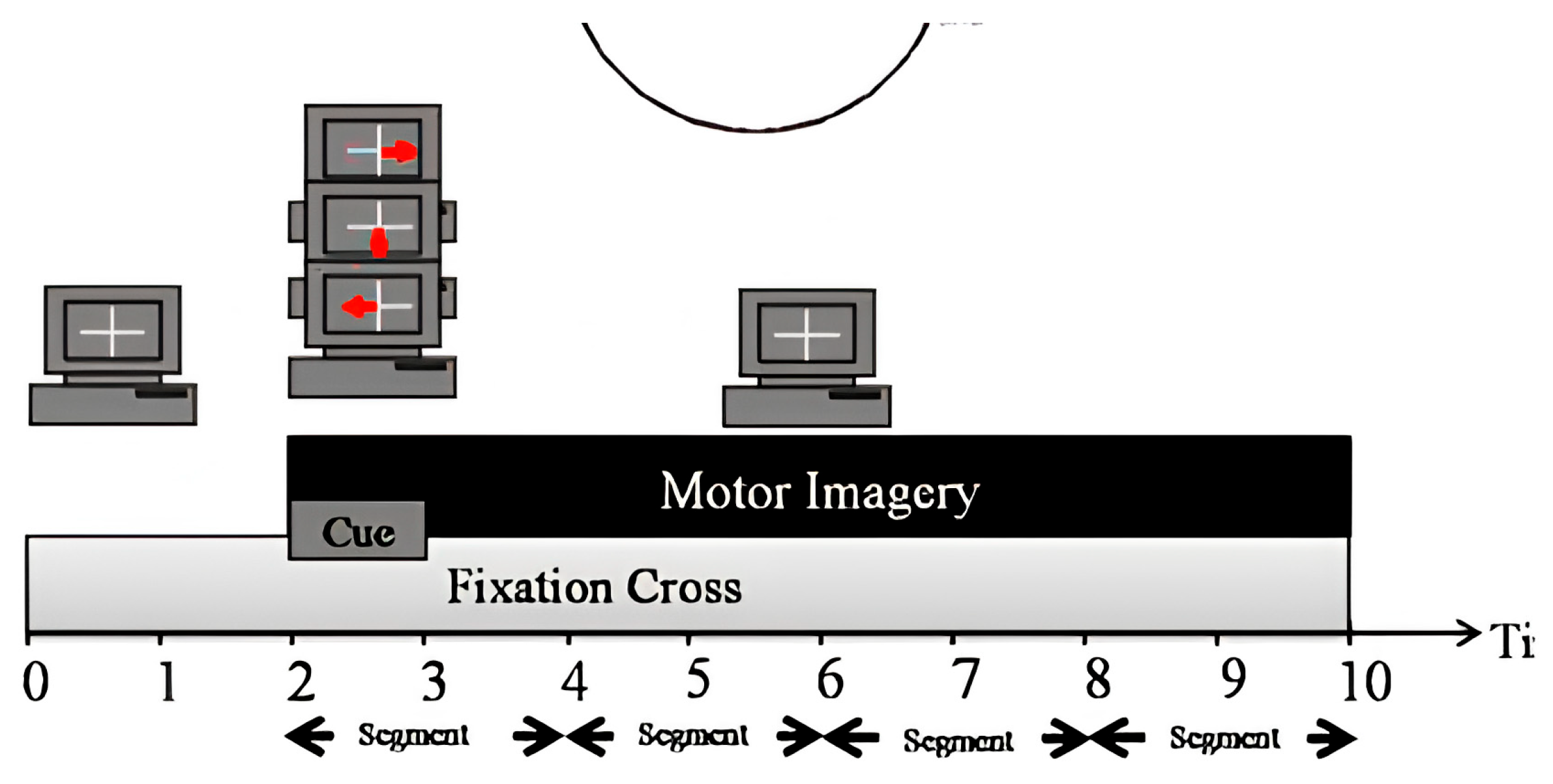
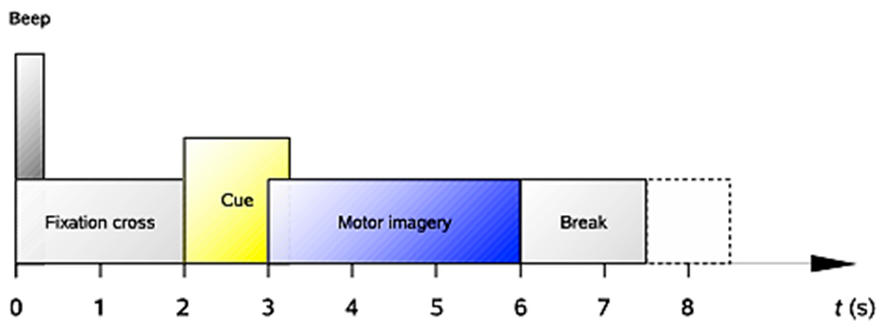
The experimental setup described [12] used five healthy male participants to evaluate the transition from offline training to real-time navigation. EEG acquisition was standardized at 256 Hz using a ProComp Infiniti™ system, with three electrodes at the C3, Cz, and C4 sites and a right ear-lobe ground. To ensure signal integrity for the mathematical analysis, electrode impedances were maintained below 1 kΩ. The system architecture employed a dual-workstation configuration connected via TCP/IP to separate real-time signal processing from VR-based feedback rendering. As detailed in the temporal sequence in Figure 3, the paradigm consisted of three sessions per subject, with each session comprising six 36-trial runs. Each 10 s trial followed a standardized progression: a fixation-cross rest period for baseline stabilization, an acoustic alert to prepare the participant, and a visual cue for left-hand, right-hand, or foot motor imagery. This structured timing provides the deterministic baseline required to evaluate the causal constraints and computational latency of the processing pipeline.

The data transmission architecture described in [17] provides a high-speed interface between the EEG hardware and the processing software. This system uses the Lab Streaming Layer (LSL) protocol to manage data synchronization and ensure low-latency streaming across the network. Raw EEG signals are sent through Bluetooth to a central server, which buffers the data and distributes it to other modules upon request.

The real-time processing is handled by the OpenViBE platform which uses a modular pipeline to filter and classify brain signals. Within this setup, the incoming LSL stream is refined by selecting specific channels (C3, Cz, and C4) and applying band-pass and notch filters to remove environmental noise. To maintain a record for future analysis, the system automatically saves the continuous data in the GDF format. A Lua-based stimulator manages the session by sending a randomized sequence of 11 different triggers, such as “left hand” or “rest.” Finally, a specialized MATLAB R2024a Connection module acts as the bridge, allowing the processed EEG data to flow directly into MATLAB for real-time analysis.

This study [14] involved 57 right-handed participants (21 male, 36 female) and was conducted under the ethics approval of the Tilburg School of Humanities and Digital Sciences. EEG data were acquired at 250 Hz using a 16-channel g. Nautilus amplifier (g.tec Medical Engineering in Schiedlberg, Austria), with electrodes positioned over the sensorimotor area (F3, Fz, F4, FC1, FC5, FC2, FC6, C3, Cz, C4, CP1, CP5, CP2, CP6, T7, and T8). The right earlobe served as a reference and AFz as the ground, with impedances maintained below 50 kΩ. Real-time signal conditioning was performed using a 48–52 Hz notch filter and a 0.5–30 Hz band-pass filter to isolate the MI frequency bands.

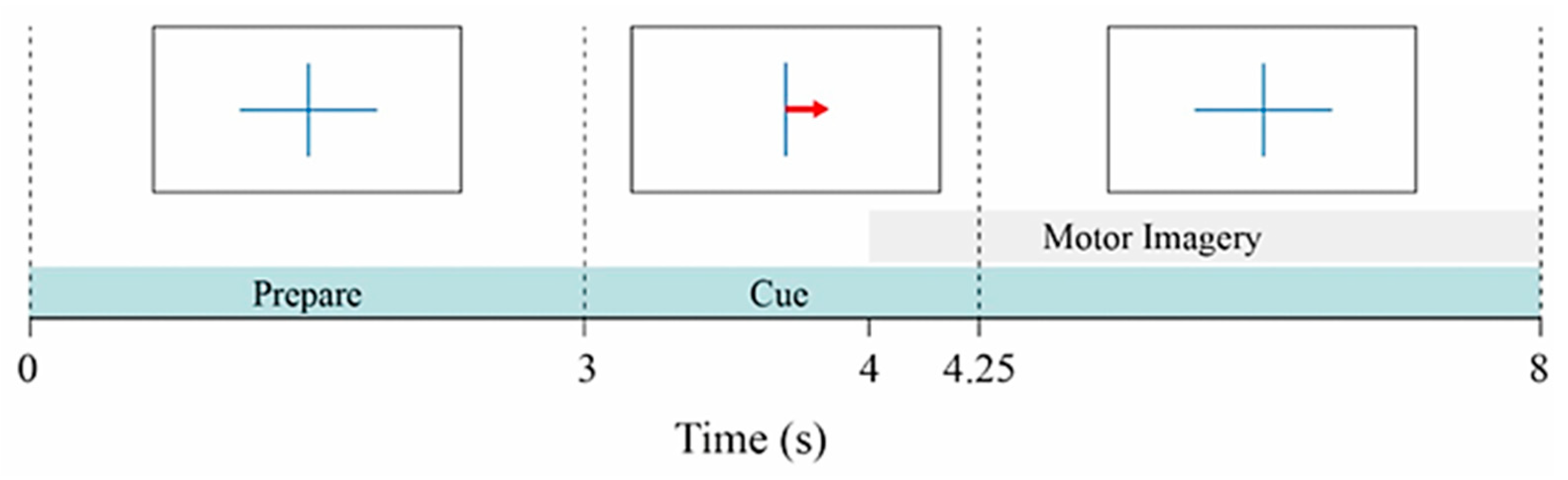
As shown in Figure 4, the experimental paradigm consisted of four runs totalling 120 trials (60 per class). The protocol began with a non-feedback screening run, followed by three runs of real-time visual feedback. Each 8 s trial followed a specific temporal sequence designed to guide the subject through the MI task. This setup provides a high-density electrode configuration and a broader demographic sample for evaluating the scalability of the processing pipeline.

• t = 0 s to 3 s: A fixation cross was presented to establish a baseline.
• t = 3 s to 4.25 s: A red arrow cued the subject to imagine squeezing either the left or right hand.
• t = 4.25 s to 8 s: During calibration runs, the fixation cross remained visible. In feedback runs, a dynamic blue bar appeared on the screen, representing the direction and certainty of the classifier’s output.

2.3.2. Datasets

To evaluate the robustness of MI pipelines against the inherent variability of EEG signals, this paper examines a diverse spectrum of benchmarks rather than a single experimental setup. This broad scope is essential for interpreting how various algorithmic architectures respond to shifts in sensor density, task complexity, and subject demographics. The methodology incorporates the BCI Competition series (III and IV) to test specific challenges in multi-class classification and spatial filtering, alongside the PhysioNet EEGMMIDB dataset. This multi-source approach provides the necessary statistical depth to evaluate intra-subject variability and the BCI illiteracy phenomenon, ensuring the findings are robust across large-scale populations and diverse data sources.

BCI Competition III Dataset 3A

The data acquisition was performed utilizing a 64-channel Neuroscan EEG amplifier (g.tec Medical Engineering in Schiedlberg, Austria), with the left and right mastoids serving as the reference and ground, respectively. The EEG signals were acquired at a sampling rate of 250 Hz and filtered with a band-pass filter between 1 and 50 Hz, followed by a notch filter. Sixty EEG channels were recorded in accordance with the configuration after which the data from all runs were concatenated and stored in the GDF format [23].

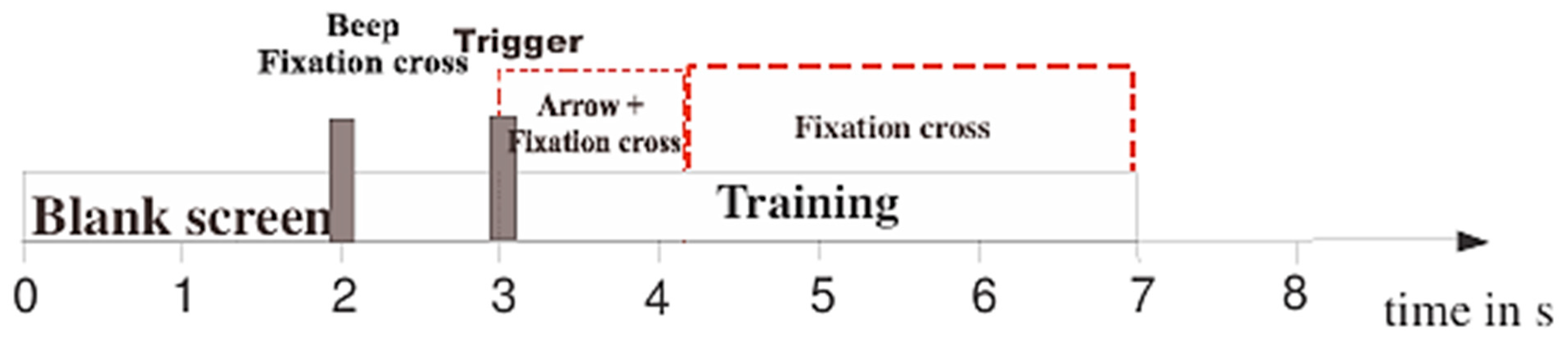
The experimental paradigm in Figure 5 involved subjects seated in a relaxed chair with armrests, tasked with performing MI of the left hand, right hand, foot, or tongue in response to randomized cues. The experiment consisted of a minimum of six runs, each containing 40 trials. The temporal sequence of each trial follows [23]:

• t = 0 s to 2 s: An initial two-second period of silence.
• t = 2 s: An acoustic stimulus and the appearance of a fixation cross (“+”) signaled the start of the trial.
• t = 3 s: A visual cue in the form of an arrow (pointing left, right, up, or down) was displayed for one second.
• t = 3 s to 7 s: The subject performed the corresponding MI until the fixation cross disappeared.

Within each run, the four distinct cues were presented ten times each in a randomized order.

BCI Competition III Dataset 3B

The data acquisition was performed utilizing a bipolar EEG amplifier from g.tec, focusing on the classification of non-stationary (time-varying) data. The EEG signals were acquired at a sampling rate of 125 Hz and filtered with a band-pass filter between 0.5 and 30 Hz, followed by a notch filter. The recording focused on the C3 and C4 positions, after which the data from all runs were concatenated and archived in the GDF format [24].

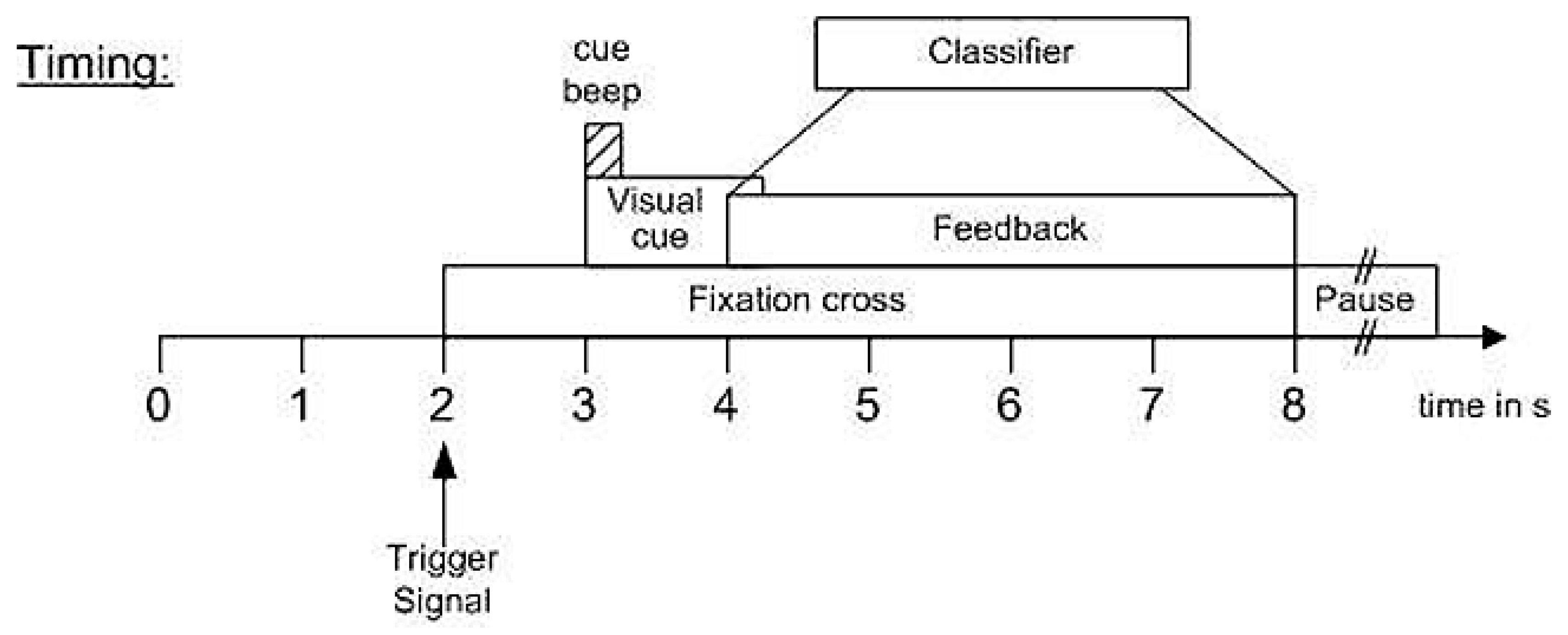
The experimental paradigm in Figure 6 involved three subjects participating in three sessions each, with each session comprising between four and nine runs. The temporal sequence of each trial, as depicted in the timing diagram, was as follows [24]:

• t = 0 ms to 2000 ms: An initial two-second baseline period.
• t = 2000 ms: A trigger signal and the appearance of a fixation cross signaled the start of the trial.
• t = 3000 ms: An acoustic stimulus (beep) and a visual cue were presented to indicate the specific imagery task.
• t = 3000 ms to 4250 ms: The visual cue remained active for a duration of 1.25 s.
• t = 4000 ms to 8000 ms: A feedback period was initiated, during which the classifier processed the data to provide real-time reinforcement to the subject.

BCI Competition III Dataset 4A

The data acquisition for this dataset was performed using five healthy subjects (aa, al, av, aw, ay) seated in comfortable chairs with armrests. The recordings consist of the four initial sessions conducted without feedback. During these sessions, visual cues were presented for a duration of 3.5 s to indicate which of the three MI tasks, left hand (L), right hand (R), or right foot (F), the subject was to perform. These task periods were separated by relaxation intervals of randomized lengths, ranging from 1.75 to 2.25 s. Two distinct methods of visual stimulation were used: (1) targets indicated by letters appearing behind a fixation cross, and (2) targets indicated by a randomly moving object. For subjects al and aw, two sessions of each stimulation type were recorded; for the remaining subjects, three sessions of type (2) and one session of type (1) were conducted [25].

The dataset is provided as continuous signals from 118 EEG channels, accompanied by markers indicating 280 cue time points for each of the five subjects (aa, al, av, aw, ay). In accordance with competition requirements, target class information is withheld (indicated by NaN values) for specific markers, and only the cues for the “right” and “foot” classes are provided for evaluation [25].

BCI Competition IV Dataset 1

The data acquisition for this dataset involved healthy subjects performing MI without feedback throughout the entire session. For each subject, two imagery classes were selected from a pool of three possibilities: left hand, right hand, and foot (with the specific foot or combination determined by the participant). The recording used 59 EEG channels. The experimental structure was categorized into calibration and evaluation phases [26]:

Calibration Phase: The first two runs utilized visual cues in the form of arrows pointing left, right, or down. Cues were presented for 4 s, during which the subject performed the indicated MI task. These periods were separated by 2 s of a blank screen and 2 s of a fixation cross. The fixation cross was superimposed on the cues, resulting in a total visibility of 6 s. These runs include complete marker information.

Evaluation Phase: Following the calibration, four subsequent runs were conducted for performance evaluation. In these runs, MI tasks were cued by soft acoustic stimuli (the words left, right, and foot) for durations varying between 1.5 and 8 s. The conclusion of each imagery period was signaled by the word stop.

BCI Competition IV Dataset 2A

The dataset used a 22-channel Ag/AgCl electrode configuration with a 3.5 cm inter-electrode distance. EEG signals were recorded monopolar at 250 Hz, referenced to the left mastoid with the right mastoid as ground. Signal conditioning included a 0.5–100 Hz band-pass filter and a 50 Hz notch filter, with amplifier sensitivity set to 100 µV. To facilitate artifact removal, three monopolar EOG channels were recorded at 250 Hz with a higher sensitivity of 1 mV. These EOG signals are intended specifically for noise mitigation during the pre-processing stage rather than for movement classification [27].

The dataset consists of nine subjects performing four MI tasks: left hand, right hand, both feet, and tongue. Data were collected across two sessions, each containing six runs of 48 trials, totaling 288 trials per session. Each session began with a five-minute EOG calibration divided into periods of eyes open (two minutes), eyes closed (one minute), and active eye movements (one minute). Notably, for subject A04T, technical constraints limited the EOG recording to the eye-movement condition only. This detailed calibration and multi-class structure serve as the baseline for auditing high-dimensional signal processing and cross-session stability [27].

Subjects were positioned in a comfortable armchair facing a computer monitor. The temporal sequence of a single trial was structured as follows in Figure 7 [27]:

• t = 0 s: The appearance of a fixation cross on a black screen and a short acoustic warning tone signaled the trial onset.
• t = 2 s: A visual cue, presented as an arrow pointing left, right, down, or up, appeared for 1.25 s to indicate the specific MI task.
• t = 2 s to 6 s: Subjects performed the cued imagery task without feedback until the fixation cross was removed at t = 6 s.
• Post-trial: A brief break followed, during which the screen remained black, before the subsequent trial commenced.

BCI Competition IV Dataset 2B

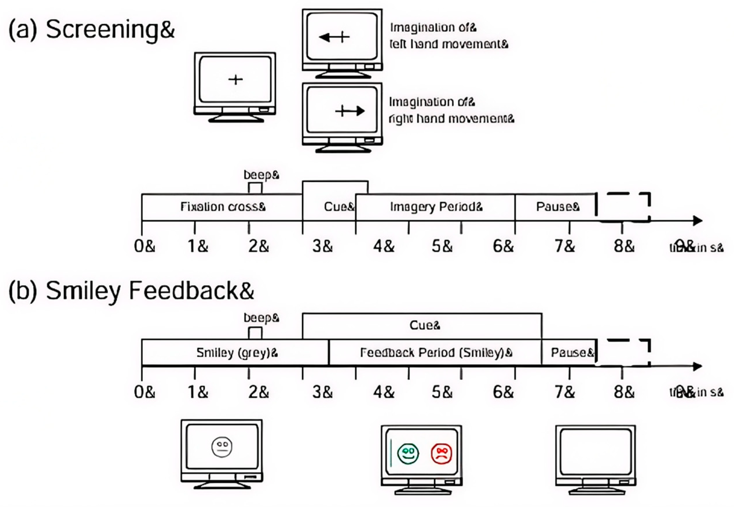
The reviewed literature involves nine right-handed subjects with normal or corrected vision, positioned in a standardized environment for multi-session evaluation. Data were collected across five sessions: two dedicated to screening (without feedback) and three focused on an online feedback paradigm. EEG was recorded through three bipolar channels (C3, Cz, and C4) at a sampling rate of 250 Hz, with filtering performed between 0.5 and 100 Hz and a 50 Hz notch filter. Notably, the system’s dynamic range was adjusted between phases, set at 100 µV for screening and 50 µV for feedback sessions to optimize signal resolution. Three monopolar EOG channels were recorded at 1 mV sensitivity to facilitate artifact processing. Each session began with a five-minute EOG calibration divided into periods of eyes-open fixation (two minutes), eyes-closed rest (one minute), and guided eye movements (one minute). This movement block utilized visual and acoustic cues to prompt specific ocular behaviors, such as blinking and rolling. This setup is particularly relevant for auditing how changes in dynamic range and EOG-based noise mitigation affect real-time classification stability [28].

The cue-based paradigm focused on two MI classes: left hand (Class 1) and right hand (Class 2) [28].

Screening Phase (Figure 8a): Each session consisted of six runs containing 20 trials each. Trials began with a fixation cross and an acoustic warning tone. After a short interval, a visual arrow pointed left or right for 1.25 s, prompting 4 s of imagery. Trials were separated by a randomized break of 1.5 s to 2.5 s.

Smiley Feedback Phase (Figure 8b): These sessions utilized four runs of 40 trials. At t = 0 s, a gray smiley appeared; at t = 2 s, a warning beep was issued. The visual cue was presented from t = 3 s to 7.5 s. During this feedback window, the smiley moved laterally based on the integrated classifier output from the previous two seconds.

Adaptive Feedback: Correct imagery shifted the smiley to a green color, while incorrect directionality turned it red. The classifier output also influenced the curvature of the smiley’s mouth, providing a qualitative “happy” or “sad” indicator of performance. Subjects were instructed to sustain the imagery task for the full duration to keep the smiley on the correct side of the screen.

PhysioNet Dataset (EEG Motor Imagery)

The PhysioNet dataset comprises over 1500 recordings from 109 subjects. Data were captured via the BCI2000 system using a 64-channel International 10–10 montage. Specific peripheral electrodes (Nz, F9, F10, A1, A2) were excluded to prioritize cortical areas relevant to MI [29].

The experimental protocol involved 14 sequential runs per subject. This included two one-minute baseline sessions (eyes open/closed) followed by twelve two-minute runs covering four motor tasks: unilateral movement (left vs. right fist) and bilateral coordination (both fists vs. both feet). For mathematical modeling, the dataset employs a tripartite annotation system (T0, T1, T2) within an EDF+ channel. T0 denotes a rest state, while T1 and T2 mark the onset of imagery or motion—representing left/right in unilateral trials and fists/feet in bilateral trials [29].

2.4. BCI Machine Learning Pipeline

The architecture of a Brain–Computer Interface (BCI) is structured as a sequential pipeline designed to transform raw neurophysiological signals into functional control commands. The process initiates with Signal Preprocessing (detailed in Section 2.4.1), where raw data is filtered to suppress noise and minimize spectral artifacts. This is followed by Feature Extraction (detailed in Section 2.4.2), which uses mathematical frameworks to translate time-varying fluctuations into a structured feature space. To refine this data, a Feature Selection stage (detailed in Section 2.4.3) is employed to isolate the most relevant information and reduce dimensionality. Finally, the processed data enters a Classification stage (detailed in Section 2.4.4), where the user’s MI is identified and the system’s reliability is quantified through rigorous performance metrics.

2.4.1. Signal Preprocessing

Following the analog-to-digital conversion, the signal undergoes digital post-processing to isolate neural activity from environmental and physiological noise. This stage uses selective digital filters to remove low-frequency drifts such as electrode movement and high-frequency artifacts such as muscle tension and electrical interference while preserving the integrity of the original raw data. By applying targeted band-pass constraints, the pipeline narrows the data to the specific frequency bands associated with MI, ensuring that the feature extraction logic focuses exclusively on the neural patterns most relevant to the user’s MI.

The choice of filter architecture is often contingent on the need for algorithmic causality and processing efficiency. Finite Impulse Response (FIR) filters are common in offline analysis; however, these filters often introduce group delays. This makes the filter less ideal for pipelines that require low latency. For this reason, Infinite Impulse Response (IIR) filters such as the Butterworth and Chebyshev topologies are standard selections because they are computationally efficient [30]. The Butterworth design is specifically valued for its maximally flat frequency response [31].

Infinite Impulse Response (IIR) Filters: These filters use internal feedback mechanisms, which results in an impulse response that theoretically continues indefinitely [30,32].

• Transfer-Function Form (H(z)): As shown by Equation (1), the filter is represented in the z-domain by the ratio of the feedforward ($B_K$) and feedback ($A_K$) coefficients. This ratio determines the placement of poles and zeros, which dictates the filter’s stability and phase response.

$$H\left(z\right)={\displaystyle \frac{{\sum }_{K=0}^{\mathrm{\infty }}{B}_K{Z}^{-K}}{1+{\sum }_{K=0}^{\mathrm{\infty }}{A}_K{Z}^{-K}}}$$

(1)

where K is the order of the filter.

• Recursive Difference-Equation Representation: In the time domain, the IIR filter is inherently recursive. As derived from the feedback coefficients in Equation (1), the current output y[n] is mathematically dependent on a weighted sum of both current/previous input samples and previous output samples. This structure is expressed as Equation (2):

$$y\left[n\right]+A_{1}y\left[n-1\right]{+\dots +A}_{K}y\left[n-K\right]=B_{0}x\left[n\right]+B_{1}x\left[n-1\right]+\dots +B_{K}x\left[n-K\right]$$

(2)

• Impulse-Response Form: The behavior of the output y[n] can also be characterized by the convolution of the input signal x[n] with the infinite impulse response h[k] in Equation (3) [30]:

$$y\left(n\right)={\displaystyle \sum _{K=0}^{\infty }}h\left(K\right)x(n-K)$$

(3)

Finite Impulse Response (FIR) Filters: In contrast to IIR designs, FIR filters do not employ feedback, ensuring that the impulse response settles to zero within a finite number of samples [30,32].

• Transfer-Function Form (H(z)): In the z-domain, the FIR filter is represented by a single polynomial consisting only of feedforward coefficients ($B_K$). As shown in Equation (4), the absence of a denominator polynomial ensures the filter remains inherently stable:

$$H\left(z\right)={\sum }_{K=0}^{N-1}{B}_K{Z}^{-K}$$

(4)

where N is the length of the filter.

• Non-Recursive Difference-Equation Representation: In the time domain, the current output y[n] is calculated solely as a weighted sum of the current and previous input samples, with no dependency on previous outputs in Equation (5):

$$y\left[n\right]=B_{0}x\left[n\right]+B_{1}x\left[n-1\right]+\dots +B_{K}x\left[n-K\right]$$

(5)

• Impulse-Response Form: The finite impulse response h[k] settles to zero after N − 1 samples. The output is defined by the finite convolution in Equation (6):

$$y\left(n\right)={\displaystyle \sum _{K=0}^{N-1}}h\left(K\right)x(n-K)$$

(6)

A key technical distinction is the use of zero-phase filtering. This technique processes data in both directions to remove phase delays [30], However, it is non-causal, as it requires access to future data points. While zero-phase filtering is mathematically robust for offline analysis, it is categorized as unsuitable for the real-time processing due to its non-causal requirements. To ensure the pipeline remains compatible with real-time processing, the filter order must be balanced. Lower-order filters are prioritized to reduce the computational workload.

The standard filtering components used in pipelines are detailed below:

High-Pass Filter: Integrated for baseline noise removal by eliminating low-frequency drifts and offsets caused by electrode-gel interfaces or bodily interference [20,33]. While highly effective at attenuating movement and perspiration artifacts, excessive high-pass filtering may result in the loss of genuine brain activity.

Low-Pass Filter: Utilized to suppress high-frequency noise and instrumental interference that exists above the neural frequency of interest [20,33]. At the specified cut-off frequency, the signal amplitude is typically reduced by 20–30% [20,33], with higher frequencies facing more aggressive attenuation or total elimination.

Band-Pass Filter: Formed by the sequential combination of high-pass and low-pass filters [20,33]. This topology isolates a specific frequency window, though fixed windows may lack the flexibility to account for individual spectral variations. In MI research, it is the primary tool for extracting the Mu and Beta bands, which contain the essential rhythmic information for task classification.

Notch Filter: Reject power-line interference, such as the common 50/60 Hz hum. In professional recording protocols, it is often recommended to initially deactivate the notch filter [20,33]. This allows technicians to identify bad electrodes or weak scalp contacts that would otherwise be masked by the filter’s rejection of the ambient electrical noise.

Traditional digital filters significantly improve the Signal-to-Noise Ratio (SNR) and are characterized by their specific efficacy when no spectral overlap exists between artifacts and neural activity. For MI, the frequency range is typically defined between 7 and 32 Hz [6]. However, experimental artifacts caused by physical motion present a challenge, as they share the same spectrum as the desired brain signals. Due to this spectral overlap, many physiological artifacts remain embedded in the data even after basic frequency filtering. In these cases, advanced techniques are necessary to remove interference without losing critical neural information.

While basic filtering is restricted to the time and frequency analysis of a single channel, advanced spatial filters evaluate the signal distribution across the entire scalp [34]. The objective is to isolate subtle electrical potentials from high-amplitude interference originating from the body or environment. Because EEG electrodes record volume-conducted noise that propagates across the scalp [35], it does not exclusively capture localized activity. Advanced spatial filters act as a mathematical lens to focus on specific regions like the Motor Cortex. This process effectively suppresses unnecessary signals from irrelevant cortical areas and prepares the data for the feature extraction stages.

Moving Average (MA): Real-time signal enhancement is achieved through the Moving Average (MA) filter [36], which minimizes computational requirements by calculating the mean of samples within a sliding window. However, the selection of the window size involves a design trade-off: while larger windows provide superior smoothing, they can degrade temporal accuracy and limit the filter’s capacity to adapt to rapid changes in the non-stationary EEG signal as defined by the discrete-time expression in Equation (7), where $y\left(t\right)$ represents the result of the Moving Average Filter at time $t$, $x(t-i)$ represents the input signal at time $(t-i)$, and $M$ represents the number of samples for computing the average, which establishes the width of the smoothing window.

$$y\left(t\right)={\displaystyle \frac{1}{M}}{\displaystyle \sum _{i=0}^{M-1}}x(t-i)$$

(7)

A systematic analysis of the technical specifications in Table 5 reveals a reproducibility gap and a lack of temporal awareness in BCI literature, where over 50% of the reviewed studies omit the filter order, effectively obscuring the response and computational complexity of their systems. This creates a conflict between reported SNR improvements and the transparency required to validate signal optimization. The use of high-order FIR filters [16] and non-causal, zero-phase, or two-pass architectures [3,13] provides a cleaner offline signal at the expense of causality, rendering such methods mathematically incompatible for real-time applications. While wide-band approaches [15] offer spectral depth, they demand high-performance BSS to manage low-frequency drifts, yet the frequent absence of reproducible coefficients makes these frameworks difficult to validate. As a result, this synthesis justifies the transition toward a more causal IIR framework as seen in the Butterworth applications of [7,14] ensuring the pipeline developed remains numerically stable and functional when used in a real-time application.

Digital filtering provides a mathematical framework for temporal signal estimation but remains limited to localized channel contexts. While effective for tracking signal dynamics, these methods are often insufficient when neural activity is spatially submerged within the high-amplitude interference sharing the same frequency spectrum. To resolve these overlapping sources, the analytical focus shifts from temporal estimation to Blind Source Separation (BSS) [37]. This methodology transitions from treating the EEG as a series of independent time-varying scalars to a multivariate vector space representation. In contrast to temporal filters that rely on correlation to suppress noise, BSS uses the spatial distribution and statistical independence of underlying generators. This move into the spatial domain is essential for unmixing scalp-level data and transforming recorded potentials back into their fundamental cortical and artefactual sources.

Variational Mode Decomposition (VMD): The decomposition of non-stationary EEG signals into band-limited modes is achieved through Variational Mode Decomposition (VMD) [38]. In contrast to data-driven approaches such as EMD, VMD characterizes each mode by its specific sparsity properties in the frequency domain while simultaneously ensuring the accurate reconstruction of the original input signal. Each extracted mode is associated with a specific, adaptively determined central frequency.

The estimation of mode bandwidth and central frequency is governed by a constrained optimization framework [38]:

• Hilbert Transform Integration: Applied to each mode to yield a unilateral frequency spectrum for analytic signal representation.
• Baseband Shifting: Each mode is shifted to its respective estimated central frequency by mixing with a tuned exponential signal.
• Bandwidth Estimation: Calculated via the squared $L^2$ norm of the gradient of the demodulated signal.

The working concept is presented in Equation (8):

$${min}_{uk,wk}=\{\sum _k{‖{\sigma }_t\left[\left(\delta \left(t\right)+{\displaystyle \frac{j}{\pi t}}\right)\ast u_k\left(t\right)\right]e^{-j{w}_{k}t}‖}_2^2\}$$

(8)

Lagrangian multipliers and quadratic penalty term are used to address the reconstruction problem which is presented as Equation (9):

$$L(u_k,w_k,\lambda )=\alpha {\sum }_k{‖{\sigma }_t\left[\left(\delta \left(t\right)+{\displaystyle \frac{j}{\pi t}}\right)\ast u_k\left(t\right)\right]e^{-j{w}_{k}t}‖}_2^2+‖f-\sum u_k‖+〈\lambda ,f-\sum u_k〉$$

(9)

The core of this architecture is the formulation of a constrained variational problem. This method aims to iteratively find the optimal set of modes that can reconstruct the original signal with minimal error; however, this iterative optimization introduces a computational overhead that must be balanced against the requirements for real-time latency.

Independent Component Analysis: Multivariate EEG signals are decomposed into independent, non-Gaussian components through Independent Component Analysis (ICA). This process is highly effective for separating brain-related signals from common artifacts such as eye blinks and muscle activity [7]. A key mathematical constraint for ICA is that the source signals must be non-Gaussian. If a component is found to be Gaussian, it is usually treated as a residual left over after the other independent sources have been extracted. While ICA is a powerful tool, applying it in real-time BCI systems is difficult. Real-time implementation of ICA is limited by the high computational cost of iterative optimization. These approaches require a careful balancing act when choosing the data block size and sensitivity settings to ensure the system remains accurate and stable during real-time [39]. Many researchers prefer to use a pre-trained unmixing matrix in training or real-time environments to keep the processing speed high because of these demands [16]; however, this introduces a generalization bottleneck, as a matrix optimized for one user may fail to isolate the independent components of another due to unique spatial and physiological differences.

The concept of ICA is as follows from Equation (10) to Equation (15):

$$\mathbf{x}\left(t\right)=[x_1\left(t\right),x_2\left(t\right),x_3\left(t\right),\dots {,x}_n\left(t\right)]$$

(10)

x$\left(\mathrm{t}\right)\in {\mathbb{R}}^{\mathrm{n}\times 1}$ is an n-dimensional EEG signal generated by hidden variables, $t=1,2,3,\dots ,T$ which indicate the length of the EEG data and T represents the number of data samples within EEG signal. $\mathit{s}\left(t\right)\in {\mathbb{R}}^{m\times 1}$ in Equation (11) is set of m-dimension random variables of independent source signals (artifacts and neural signal) contained in $\mathit{x}\left(t\right)$ with the condition that number of dimensions in the random variables should be less than the number of dimensions in EEG signal.

$$\mathbf{s}\left(t\right)=[s_1\left(t\right),s_2\left(t\right),s_3\left(t\right),\dots {,s}_m\left(t\right)](m\le n)$$

(11)

$${\mathbf{x}}_i\left(t\right)={\displaystyle {\sum }_{j=1}^n}{a}_{ij}{s}_j\left(t\right),(i=1,2,3,\dots ,n;j=1,2,3,\dots ,m)$$

(12)

The linear model of ICA is shown by Equation (13) which is the expansion of Equation (14) where ${\mathbf{s}}_i\left(t\right)$ is the independent component and $\mathit{A}\in {\mathbb{R}}^{n\times m}$ is the mixing matrix:

$$\left[\begin{array}{c}{x}_1\left(t\right)\\ ⋮\\ x_n\left(t\right)\end{array}\right]=\left[\begin{array}{ccc}{a}_{11}& \dots & a_{1m}\\ ⋮& \ddots & ⋮\\ a_{n1}& \dots & a_{nm}\end{array}\right]\left[\begin{array}{c}{s}_1\left(t\right)\\ ⋮\\ s_m\left(t\right)\end{array}\right]$$

(13)

$$\mathbf{x}\left(t\right)=\mathbf{A}\mathbf{s}\left(t\right)$$

(14)

The goal of ICA is to find a linear transformation matrix known as the unmixing matrix W based on the assumption that sources are statistically independent of each other [9]. After the linear transformation of x, n-dimensional column vectors z(t) is obtained and made approximately and as accurately as possible as the source signal s(t) which becomes an estimate of s(t) as shown in Equation (15):

$$\mathbf{z}\left(t\right)=\mathbf{W}\mathbf{x}\left(t\right)=\mathbf{W}\mathbf{A}\mathbf{s}\left(t\right)$$

(15)

Empirical Mode Decomposition (EMD): Artifact removal and feature extraction are facilitated by decomposing complex EEG signals into hierarchical Intrinsic Mode Functions (IMFs) through Empirical Mode Decomposition (EMD). These IMFs represent the various hierarchical levels into which the EEG signal is partitioned, each corresponding to the underlying frequency distribution of the data. The extraction of these functions is achieved through a recursive sifting process [8,36]. For a component to be mathematically defined as an IMF, it must satisfy two specific criteria [40,41]:

• Extrema and Zero-Crossings: The total number of local extrema and zero-crossings must be equal or differ by no more than one.
• Symmetry of Envelopes: The local mean of the upper and lower envelopes, defined by local maxima and minima respectively, must be zero at every point in the time series.

The iterative nature of the sifting process introduces a variable computational burden to a BCI pipeline. Because the algorithm must recursively process the data until each IMF satisfies the formal convergence criteria, the system is subject to stochastic latency. In contrast to fixed-order filters, the processing time per epoch is non-deterministic, fluctuating according to the SNR and the underlying complexity of the non-stationary EEG input. A primary limitation of EMD is mode mixing: a single IMF contains signals of widely different frequencies, or a signal of a similar frequency is spread across multiple IMFs, potentially reducing the robustness of subsequent feature extraction.

The working operation of EMD is shown from step 1 to step 9:

Step 1: Lower and upper peaks of signal are located.

Step 2: To produce the upper and lower curvature, cubic spline interpolation is done to join lower and upper peaks of signal.

Step 3: Average $h_1\left(t\right)$ of the two curvature is calculated and the difference is calculated in Equation (16) where x(t) represents the EEG signal and $c_1\left(t\right)$ represents the difference in signal and curvature average.

$$c_1\left(t\right)=x\left(t\right)-h_1\left(t\right)$$

(16)

Step 4: $c_1$ is the modualated mode of x(t) if it satisfies the condition of IMF, however if $c_1$ is not an IMF, steps 1–3 are repeated on $c_1$ resulting in Equation (17):

$$c_{11}\left(t\right)=c_1\left(t\right)-h_{11}\left(t\right)$$

(17)

where $h_{11}\left(t\right)$ is the upper and lower average value of $c_1$.

Step 5: $c_{1j}\left(t\right)$ becomes an IMF after repeated sifting iterations represented by j as shown in Equation (18):

$$c_{1j}\left(t\right)=c_{1\left(j-1\right)}\left(t\right)-h_{1j}\left(t\right)$$

(18)

It is labeled as the first IMF module of the original data represented by $i_1=c_{1j}$

Step 6: By subtracting the IMF module from the signal as shown in Equation (19) where $d_1$ becomes the original signal for the next loop.

$$d_1=x\left(t\right)-i_1\left(t\right)$$

(19)

These steps are continued until a certain number of IMFs are obtained along with the final residue of $d_N$ which is the mean trend of the EEG signal x(t). The original signal can be reconstructed using Equation (20):

$$x\left(t\right)={\displaystyle \sum _{n=1}^N}{i}_n\left(t\right)+d_N(t)$$

(20)

Artifact Subspace Reconstruction: Artifact Subspace Reconstruction (ASR) provides a non-iterative alternative to ICA for artifact rejection, optimized for high-speed processing. By utilizing Principal Component Analysis (PCA) and sliding-window statistics, ASR identifies and subtracts the artifact subspace without the computational overhead of an iterative search for statistical independence. This allows the pipeline to dynamically adapt to non-stationary noise, such as sudden muscle bursts, ensuring stability in real-time MI applications. The ASR algorithm identifies and removes non-stationary artifacts through a three-stage process. Reference data is established by calculating channel-wise root-mean-square (RMS) values in 1 s windows and concatenating segments with z-scores between −3.5 and 5.5. An IIR filter is applied to this reference to suppress brain oscillations while the covariance matrix undergoes eigenvalue decomposition. This determines rejection thresholds in principal component space based on the mean and standard deviation of component RMS values [42].

Finally, the same IIR filter and eigenvalue decomposition are applied to uncleaned EEG segments along a sliding window. Components exceeding the established thresholds in the PC space are set to zero. The underlying concept of ASR is that a data segment can be decomposed into latent components using a mixing matrix [42] as shown in Equation (21):

$$x_t=M_r{S}_t$$

(21)

where $x_t$ is the EEG data segment, $M_r$ is the mixing matrix and $S_t$ is the latent components. The mixing matrix is determined from a clean reference segment such that its relationship to the reference covariance is $M_r{M}_r^T=Cov\left(x_{ref}\right)$. To identify which components in $S_t$ are artifacts, a threshold $T_i={\mu }_i+k·{\sigma }_i$ is calculated from a clean reference segment, where k is a user-defined parameter, ${\mu }_i$ is the mean and ${\sigma }_i$ is the standard deviation of RMS values.

Artifact rejection is performed in the principal component space, allowing the clean latent components to be reconstructed using the Moore–Penrose pseudoinverse of the truncated mixing matrix [42] as shown from Equation (22) to Equation (24):

$$Y_t=V_t^T{x}_t=V_t^T{M}_r{S}_t$$

(22)

$${\left(S_t\right)}_{clean}=({V_t^T{M}_r)}_{trunc}^{+}{Y}_t=({V_t^T{M}_r)}_{trunc}^{+}{V}_t^T{x}_t$$

(23)

The cleaned signal is then reconstructed, as defined by the mathematical operations in Equation (24). This automated approach allows for the isolation of the artifact subspace while preserving the underlying neural signal integrity [42].

$${\left(X_t\right)}_{clean}=M_r({V_t^T{M}_r)}_{trunc}^{+}{V}_t^T{x}_t$$

(24)

Riemannian Artifact Subspace Reconstruction (rASR): Geometric variance overestimation, commonly known as the swelling effect, is addressed through the Riemannian Artifact Subspace Reconstruction (rASR) framework [16]. While standard ASR operates in Euclidean space, it often suffers from the swelling effect, a variance overestimation that occurs when the curved geometry of the EEG covariance manifold is ignored. By treating the EEG signal as a point on the Symmetric Positive Definite (SPD) manifold, rASR utilizes Riemannian metrics to maintain the structural integrity of the neural data:

1. Robust Covariance Estimation: As defined in Equation (25), a robust, unbiased estimator of the sample covariance is computed for each data segment. This optimization allows the algorithm to perform a single decomposition per window, ensuring that the computational complexity remains linear relative to the number of windows, even when handling the complex geometry of the Riemannian manifold.

$$C_i={\displaystyle \frac{1}{n-1}}{X}_i{X_i}^T$$

(25)

where $n_{data}$ is the number of samples in the current data segment and $X_i\in R^{c\times n_{data}}$ is the current channel matrix of $n_{data}$ samples and c channels.

2. Geometric Averaging (Karcher Mean): The Euclidean running mean is replaced by the Riemannian center of mass, as shown in Equation (26). By minimizing the sum of squared geodesic distances, the average covariance remains on the manifold, preserving the true structure of the neural signal.

$$\overline{C}={argmin}_{C\in P\left(c\right)}{\displaystyle \sum _{i=0}^N}{\delta }_R^2(C,C_i)$$

(26)

where ${\delta }_R$ is the geodesic Riemannian distance and P(c) is the manifold of c × c symmetric positive definite (SPD) matrices.

3. Principal Geodesic Analysis (PGA): Dimensionality reduction is performed via PGA rather than standard PCA. By projecting data onto geodesic submanifolds, PGA more accurately captures the high variance associated with artifacts in curved spaces, leading to superior suppression of non-neural components.

To ensure cross-sectional consistency, the qualitative assessments in

Table 6. Comparative Evaluation of Preprocessing and Decomposition Methodologies.

Method	Robustness	Computational Complexity	Latency	Interpretability	Generalizability
Digital Filtering	Low	Minimal	Near Zero	High	Moderate
Moving Average	Low	Minimal	Low	High	Low
VMD/EMD	High	High	Moderate	Moderate	Moderate
ICA	Moderate	High	High (Batch)	High	Low
ASR	High	Moderate	Low	Moderate	High
rASR	Very High	Moderate	Low	Moderate	Very High

are synthesized from the algorithm logic and operation identified throughout this technical audit. These evaluations follow the criteria established in Appendix A (

Table A2. Definition of Operational Ranking Metrics.

Rating	Latency and Complexity	Robustness and Generalizability	Interpretability
Near-Zero/Minimal	Sample-based operations; requires no data buffering or iterative cycles.	Static-domain logic; assumes idealized signal conditions with no adaptive correction.	Direct Mapping; the output is a first-order linear function of the raw input.
Low/Moderate	Window-based or recursive architectures; requires short-term data stabilization/kernels.	Benchmark-stable; effective under controlled conditions but sensitive to SNR outliers.	Mixed Transparency; requires secondary mapping or statistical visualization to interpret.
High/Very High	Block-buffered (Batch) or multi-branch architectures with high parameter/iterative overhead.	Designed to isolate signal from non-stationary noise.	Physiologically meaningful; results correlate to known brain regions or patterns.

) and represent a descriptive analysis of the existing literature; they are not intended as empirical benchmarks derived from a singular experimental study.

The comparative profiles in Table 6 highlight a notable trade-off between interpretability and robustness. While traditional frameworks such as Digital Filtering and Moving Averages provide the minimal complexity and near-zero latency required for real-time control, the analysis suggests these approaches encounter limitations in accounting for the non-stationarity of EEG signals. In contrast, high-order decomposition methods such as VMD/EMD and ICA offer enhanced noise rejection but exhibit computational bottlenecks and latency, often requiring batch processing that is unsuitable for real-time control. Artifact Subspace Reconstruction (ASR) and its Riemannian variant (rASR) are identified within this descriptive framework as balanced solutions. These methods demonstrate a capacity for high generalizability across subjects and sessions while maintaining the low-latency profile necessary for transitioning laboratory benchmarks into reliable, real-world assistive technologies.

The technical landscape summarized in

Table 7. Technical Specifications of Blind Source Separation (BSS) and Signal Decomposition Methods in MI Reviewed Literature.

Paper	Year	BSS	Decomposition Method	Standalone/Hybrid	Notes
[12]	2015	None Specified	None Specified	-	Absence of BSS leaves the system vulnerable to artifact contamination
[16]	2019	ASR rASR	None Specified	Standalone Standalone	Uses Riemannian Artifact Subspace Reconstruction to clean eye-blinks without the high latency of full ICA.
[3]	2020	None Specified	None Specified	-	Relied on filtering to remove noise and artifacts.
[13]	2021	ICA ICA	None Specified Wavelet Transform	Standalone Hybrid	DWT decomposes signals into sub-bands before ICA, allowing for targeted noise removal in specific frequency ranges.
[14]	2022	None Specified	None Specified	-	Use of deep learning model allows for end-to-end processing.
[15]	2023	None Specified	None Specified	-	Use of deep learning model allows for end-to-end processing.
[19]	2023	None Specified	None Specified	-	Decomposed Signal into sub-bands using Filtering.
[7]	2023	ICA	None Specified	Standalone	Relies on the statistical independence of brain vs. non-brain sources; effective for stationary artifact removal.
[17]	2024	None Specified	None Specified	-	Use of deep learning model allows for end-to-end processing.
[18]	2024	None Specified	None specified	-	Decomposed Signal into sub-bands using Filtering.

reveals a divide between traditional signal processing and modern black-box approaches. While the majority of reviewed studies omit formal Blind Source Separation (BSS), this is often a deliberate architectural choice in papers using Deep Learning. In such frameworks, spatial filtering and artifact isolation are mathematically embedded within the convolutional layers, reducing the need for a standalone BSS stage. However, this end-to-end reliance often sacrifices mathematical interpretability and introduces computational costs that can impede real-time execution. By contrast, the Hybrid ICA-Wavelet Transform (WT) seen in [3] and the subspace reconstruction methods in [16] offer a more transparent and modular alternative.

2.4.2. Feature Extraction

Post-artifact suppression, the pipeline transforms multi-dimensional time series into a discriminative feature space. This stage functions as a dimensionality reduction task, compressing high-dimensional electrode data into a condensed vector that represents neural intent while discarding redundant noise. The process targets the spatial and temporal dynamics of sensorimotor rhythms, specifically Mu and Beta oscillations. Since these rhythms are identified by localized power changes, the framework calculates scalp-wide variance to detect movement imagination. Precision is critical as information loss at this stage creates a bottleneck for classification accuracy.

(a)

Time Domain

• Autoregressive Models: Autoregressive models are founded on the principle that signals naturally tend to be correlated over time or across other dimensions. As a result, it is possible to predict future measurements based on a sequence of preceding values [43,44]. The AR model prediction of the current signal measurement, derived from these past values, is represented by Equation (27):

$$x\left(n\right)=e\left(n\right)-a\left(1\right)x\left(n-1\right)-a\left(2\right)x\left(n-2\right)-\dots -a\left(n\right)x(n-r)$$

(27)

where x(n) is the input EEG signal, a(n) are the AR parameters, r is the model order, and e(n) are the prediction errors. In the context of feature extraction, the signal is represented by the resulting AR coefficients. The robustness of these coefficients is inherently limited by the non-stationary nature of EEG, as the model may fail to maintain intra-subject consistency over long recording sessions. These coefficients possess the advantage of remaining invariant even when the data undergoes scaling changes. A significant challenge in this approach involves determining the optimal order of the model. An order that is too low fails to represent the data accurately, whereas an excessively high order results in increased noise [36,45].

(b)

Frequency Domain

• Fast Fourier Transform (FFT): Power distribution within the Mu and Beta frequency bands is quantified through the Fast Fourier Transform (FFT). It provides a spectral representation essential for MI analysis. It serves as a high-speed algorithm for computing the Discrete Fourier Transform (DFT) or its inverse [33]. Mathematically, the DFT transforms a sequence of $N_{real}$ real or complex numbers x[n] into a series of complex-valued frequency components X(k), as defined by the following Equation (28):

$$X\left(k\right)={\displaystyle \sum _{n=0}^{N_{real}-1}}x[n]e^{-{\displaystyle \frac{j2\pi kn}{N_{real}}}}$$

(28)

The FFT reduces computational complexity by decomposing the DFT matrix into sparse factors, making it efficient for real-time processing of narrowband, stationary signals. However, the FFT is limited in EEG analysis due to its assumption of signal stationarity, which prevents the simultaneous extraction of frequency components and their temporal locations. As a result, it cannot capture the non-stationary dynamics of the EEG signal or reveal the spatial distribution of neural generators across the scalp [33].

(c)

Time-Frequency Domain

• Wavelet Transform: Intra-subject robustness in MI is enhanced through the Wavelet Transform (WT), which captures both temporal and spectral transients within non-stationary signals [33]. This allows the feature space to remain stable across different trials for the same user, even when the timing of their MI varies slightly. Within this framework, the wavelet transform is categorized into two primary types: Continuous Wavelet Transform (CWT) and Discrete Wavelet Transform (DWT):

The Continuous Wavelet Transform (CWT) facilitates the projection of a signal into the time-frequency domain. This method is characterized as continuous as the translation and scale parameters of the wavelets are varied in a continuous manner. As a result, the transform produces a continuously varying set of coefficients, which results in a redundant representation of the signal [43,45]. The CWT can be represented by Equation (29):

$$X\left(a,\tau \right)={\displaystyle \frac{1}{\sqrt{a}}}{\int }_{+\infty }^{-\infty }x\left(t\right)\phi \ast \left({\displaystyle \frac{t-\tau }{a}}\right)dt$$

(29)

where x(t) is the EEG signal, $\phi$ is the mother wavelet represented by Equation (30), a is the scale parameter, and $\mathsf{\tau }$ is the shift parameter.

$$\{\phi \left({\displaystyle \frac{t-\tau }{a}}\right),\left(a,\tau \right)\in R^T\times R\}$$

(30)

where $a=2^{-j}$ and $\tau =k{2}^{-j}$ where k and j are integers. Choosing a and $\tau$ requires critical sampling which gives a sparse matrix where most of its elements are zeros.

The Discrete Wavelet Transform (DWT) algorithm decomposes a signal into low-frequency and high-frequency coefficients, referred to as approximation coefficients represented by Equation (31) and detail coefficients represented by Equation (32). Compared to the CWT, the DWT requires less computational time and provides a non-redundant representation of the signal.

$$W_{\vartheta }\left(j_0,k\right)={\displaystyle \frac{1}{\sqrt{M_p}}}\sum _{x}f\left(x\right){\vartheta }_{j_0,k}(x)$$

(31)

$$W_{\phi }\left(j,k\right)={\displaystyle \frac{2}{\sqrt{M_p}}}\sum _{x}f\left(x\right){\phi }_{j,k}(x)$$

(32)

where $\vartheta \left(x\right)$ is the scaling function, $\phi \left(x\right)$ is the wavelet function, and $M_p$ is the power of 2.

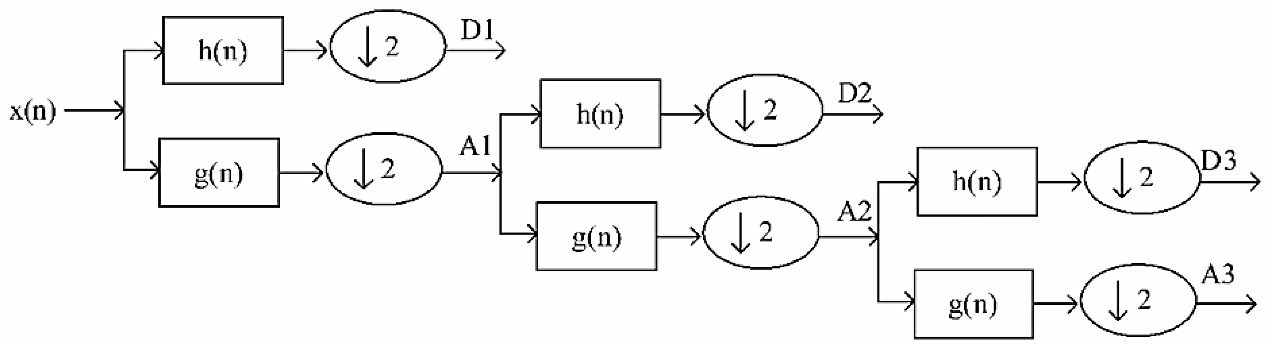
As shown in Figure 9, the multi-resolution framework processes signals using dual digital filters and down-samplers by a factor of 2. In this architecture, the discrete mother wavelet h[n] functions as a high-pass filter, while its mirror version g[n] serves as a low-pass filter. The downsampled outputs of these initial filters produce the first level of detail D1 and approximation A1. This decomposition continues by iteratively processing each subsequent approximation until a predetermined level is reached.

The specific number of decomposition levels is selected to ensure that the signal correlates with the frequency bands required for classification. To determine these levels, the frequency range of each detail scale is calculated relative to the sampling frequency of the original signal [46], as shown in Equation (33), where the full range of the signal is defined by the governing sampling equation.

$$\{\left[0,{\displaystyle \frac{f_s}{2^{l+1}}}\right];\left[{\displaystyle \frac{f_s}{2^{l+1}}},{\displaystyle \frac{{2f}_s}{2^{l+1}}}\right];\left[{\displaystyle \frac{{2f}_s}{2^{l+1}}},{\displaystyle \frac{3f_s}{2^{l+1}}}\right];\left[{\displaystyle \frac{{3f}_s}{2^{l+1}}},{\displaystyle \frac{4f_s}{2^{l+1}}}\right];\dots ;\left[{\displaystyle \frac{\left(2l-1\right)f_s}{2^{l+1}}},{\displaystyle \frac{f_s}{2}}\right]\}$$

(33)

where $f_s$ is the sampling frequency, and l is the level of decomposition.

(d)

Spatial Domain

Common Spatial Patterns (CSP): Event-Related Synchronization (ERS) and Event-Related Desynchronization (ERD) are isolated from MI through the Common Spatial Patterns (CSP) algorithm. The algorithm maximizes the variance of spatially filtered signals for one class while simultaneously minimizing it for the other, effectively separating the two classes based on their respective variances [7]. While the standard CSP framework is designed for binary classification, it is extended to multiclass paradigms using strategies such as One-vs-Rest (OVR) or Joint Approximate Diagonalization (JAD). In these contexts, the algorithm decomposes multiple covariance matrices to identify spatial filters that distinguish one specific task from the aggregate of all other classes. This extension is essential for high-density architectures involving multiple MI tasks, such as foot, tongue, and hand movements [34]. While these multiclass extensions increase computational complexity, they maintain robustness by isolating task-specific variances, provided the system is calibrated to the individual subject’s unique spatial topography.

The procedure for binary CSP begins by computing normalized spatial covariance matrices for each trial. These are averaged across all trials to derive the class-specific covariance matrices, ${\overline{R}}_1$ and ${\overline{R}}_2$. Finally, a composite covariance matrix $R$ is formulated by summing these two averaged matrices, as represented by Equation (34).

$$R={\overline{R}}_1+{\overline{R}}_2=U_0\sum U_0^T$$

(34)

where $U_0$ is the eigenvectors and $\sum$ is the diagonal matrix of the corresponding eigenvalues.

A whitening transformation matrix, P, is obtained by summing the eigenvalues and the eigenvectors of the covariance matrix R as represented by Equation (35):

$$P={\sum }^{-{\displaystyle \frac{1}{2}}}{U}^T$$

(35)

P matrix transforms the normalized spatial covariance matrices R1 and R2 into another space, as shown in Equations (36) and (37). The sum of the corresponding eigenvalues is always equal to 1, as shown by Equation (38):

$$S_a=P{\overline{R}}_1{P}^T$$

(36)

$$S_b=P{\overline{R}}_2{P}^T$$

(37)

$$1=\sum a+\sum b$$

(38)

The spatial covariance matrices form a common eigenvector, $U^T$, which then along with the whitening transformation matrix, P, forms a spatially filtered signal, $W_{spatial}$, as given in Equation (39):

$$W_{spatial}=U^{T}P$$

(39)

For a dataset with n channels, the transformation matrix $W$ is defined as an $n\times n$ matrix where rows represent spatial patterns. These patterns identify the most significant weighted channel values, allowing for the truncation of redundant information and a reduction in data dimensionality by disregarding non-contributory values.

• Principal Component Analysis (PCA): Downstream computational complexity and the curse of dimensionality are mitigated through Principal Component Analysis (PCA). By projecting high-dimensional electrode data into a lower-dimensional subspace, PCA significantly reduces downstream computational complexity and mitigates the risk of the curse of dimensionality during classification. PCA identifies principal components obtained from the decomposition of the eigenvalue and eigenvector covariance matrices [41,47]. PCA will form a new dimension that is ranked based on the variance of the data. The transformation of the multivariate EEG signal into this reduced subspace is governed by the following orthogonal projection:

(1) Mean of the data is calculated within each dimension using Equation (40):

$$\dot{X}={\displaystyle \frac{1}{n_{data}}}{\displaystyle \sum _{i=1}^{n_{data}}}{x}_i$$

(40)

where $x_i$ is the sample data.

(2) Covariance matrix is calculated using Equation (41):

$$C_x={\displaystyle \frac{1}{n-1}}{\displaystyle \sum _{i=1}^n}(x_i-\dot{X})(x_i-\dot{X}{)}^T$$

(41)

where $C_x$ is the covariance matrix.

(3) The eigenvectors and eigenvalues of the covariance matrix are computed using Equation (42):

$$C_x{v}_m={\lambda }_m{v}_m$$

(42)

where $v_m$ is eigenvectors and ${\lambda }_m$ is the eigenvalues

(4) The eigenvectors and eigenvalues are sorted in descending order. A principal component is a series of eigenvectors according to the order of eigenvalues in stage 3.

(5) A new dataset is generated.

The evaluative audit in

Table 8. Comparative Evaluation of Feature Extraction Methodologies.

Method	Robustness	Computational Complexity	Latency	Interpretability	Generalizability
Autoregressive Model	Moderate	Minimal	Near Zero	High	Moderate
FFT	Low	Minimal	Low	High	Low
WT	High	High	Moderate	Moderate	Moderate
CSP	Moderate	Moderate	Near Zero	High	Low
PCA	Moderate	Moderate	Near Zero	Moderate	Low

(defined by criteria in Table A2) presents the technical parameters identified in the transition from raw neural signals to discriminative features. While the Fast Fourier Transform (FFT) is characterized by minimal computational overhead, its algorithmic reliance on signal stationarity is observed as a constraint relative to the Wavelet Transform (WT). Within the scope of this audit, WT demonstrates a capacity for capturing transient MI dynamics, though it typically presents a higher processing demand. In the spatial domain, Common Spatial Patterns (CSP) is noted for its interpretability; however, the analysis suggests that both CSP and PCA exhibit limited generalizability across the reviewed frameworks. Because these spatial filters are optimized for subject-specific brain geometries, they frequently necessitate recurring calibration to maintain stability across different sessions.

A critical evaluation of

Table 9. Technical Specifications of Feature Extraction Methodologies and Mathematical Domain Representations across Reviewed Literature.

Paper	Year	Domain	Extraction Method	Number of Features	Notes
[12]	2015	Time, Time-Frequency	FFT, AR, MA Model, ARMA, DCT, DST	48	High feature count to 5 subjects suggests potential overfitting to stochastic noise
[16]	2019	None Specified	None Specified	-	Restricted to BSS implementation
[3]	2020	Spatial	CSP	32	By using 32 features for 118 electrodes, it performs significant data compression, focusing only on the most discriminative spatial variances
[13]	2021	Spatial	CSP	120	120 features are extremely high for real-time BCI. It includes a risk of overfitting and curse of dimensionality.
[14]	2022	Spatial	CSP	-	Omitted feature count prevents assessment of the model’s structural risk or real-time latency.
[15]	2023	None Specified	None Specified	-	Use of deep learning model allows for end-to-end processing.
[19]	2023	Spatial	CSP	40	Provides a transparent, moderate feature count.
[7]	2023	Spatial	CSP Log-Variance	-	Omission of feature count introduces ambiguity regarding model overfitting and prevents computational auditing.
[17]	2024	Spatial	Auto selected regularized CSP	-	Auto-selection without a final count prevents verification of real-time processing boundaries
[18]	2024	Spatial	CSP	40	Provides a transparent, moderate feature count.

reveals in the spatial domain, Common Spatial Patterns (CSP) remains the acknowledged standard for Motor Imagery. There is a systemic lack of mathematical transparency across the reviewed literature. Reference [15] exhibits a total omission of extraction logic, making it impossible to validate the dimensionality of the data entering the classification stage. Among the papers that do provide specifications, there is no consensus on feature density; Refs. [3,19] employ targeted sets of 24 to 32 features to maintain computational efficiency, whereas [13] uses an extremely high-dimensional set of 120 features, which increases the risk of the curse of dimensionality and overfitting without aggressive regularization. More recent entries such as [7,17] attempt to address these mathematical instabilities through log-variance transformations and Regularized CSP (RCSP) to improve covariance estimation. The data in Table 7 suggests that without specific selection strategies, high-resolution spatial maps likely impose an excessive computational load that would compromise the latency of a system.

2.4.3. Feature Selection

Feature selection mitigates the Curse of Dimensionality, where input variables from channels, frequency, and time exceed available training trials to prevent overfitting to noise rather than neural intent. This ensures a robust mapping of MI tasks.

Filter feature selection methods act as a preprocessing stage, ranking features through statistical properties such as Mutual Information (MI) or Pearson correlation independent of the classifier [48]. Features failing to meet a set threshold are discarded. In contrast, Wrapper feature selection methods use the classifier as a black box, iteratively testing feature subsets to maximize classification accuracy [49]. While more tailored to the model’s decision boundary, Wrappers are computationally intensive and prone to overfitting, making them better suited for offline training rather than real-time BCI loops.

Relief-F: Feature relevance in noisy or incomplete EEG datasets is determined through the Relief-F framework [18,50]. This filter-based approach evaluates how effectively a variable differentiates between classes by analyzing discrepancies in feature values between pairs of nearest-neighbor instances. Because the algorithm operates independently of other features, it is particularly suited for enhancing classification performance in multi-class MI paradigms where redundant or low-relevance features may degrade accuracy. Subsequent extensions have focused on improving scalability, adapting to diverse data types, and increasing overall computational efficiency. The specific mathematical weight updates for these features are defined through the sequence of Equation (43) to Equation (46).

If $x_G$ and $x_H$ features belong to the same class, the weight update formula is represented by Equation (43):

$$w_{ji}=w_{ji}-{\displaystyle \frac{{\Delta }_j(x_G,x_H)}{M_{iter}·d_{GH}}}$$

(43)

If $x_G$ and $x_H$ features belong to different classes, the weight update is represented by Equation (44):

$$w_{ji}=w_{ji}+{\displaystyle \frac{p_{yH}\left(1-p_{yG}\right)·{\Delta }_j(x_G,x_H)}{M_{iter}·d_{GH}}}$$

(44)

where $w_{ji}$ is the weight of the predictor, ${\Delta }_j(x_G,x_H)$ is the absolute difference between the jth feature of $x_G$ and $x_H$, $p_{yH}$ and $p_{yG}$ denote the prior probabilities of the classes associated with instances H and G, respectively, $M_{iter}$ is the number of iterations and $d_{GH}$ is a scaled distance between $x_G$ and $x_H$ defined by Equation (45):

$${\tilde{d}}_{GH}=e^{{-({\displaystyle \frac{rank\left(G,H\right)}{\sigma }})}^2}$$

(45)

where rank(G, H) represents the ordinal position of observation H within the nearest neighbors (k) of observation G, sorted by distance and $\sigma$ is a parameter that affects the scaling. Total distance $d_{GH}$ can be calculated by Equation (46):

$$d_{GH}={\displaystyle \sum _{l=1}^k}{\tilde{d}}_{Gl}$$

(46)

Infinite Feature Selection (InFS): Feature importance is evaluated through the convergence of a power series of matrices in the Infinite Feature Selection (InFS) framework [18]. In this graph-based architecture, features are modeled as nodes and their relationships as edges, where feature subsets are treated as paths of infinite length. The algorithm assigns scores to each node based on its visit frequency across all possible paths. This allows InFS to determine a feature’s relevance by considering it within the context of all other feature combinations rather than in isolation.

In the context of pairwise feature analysis, consider a set of feature distributions F = {f(1), …, f(n)} and a sample $x\in R$ representing a distribution f. To characterize the interdependencies within this feature space, the system is modeled as an undirected fully connected graph $B=\left(V,E\right)$. Here, V represents the collection of vertices for individual feature distributions, while the edge set E comprises weighted edges that quantify the pairwise relationships between them. The topological structure and the associated pairwise energy terms are mapped to the adjacency matrix, ${\mathit{A}}_{\mathit{a}\mathit{d}\mathit{j}}$ of G as defined in Equation (47) [51]:

$${{(A}_{adj})}_{ij}={\lambda \%}_{ij}+(1-\lambda )p_{ij}$$

(47)

where $\lambda$ is the loading coefficient in the range $\lambda \in$ [0, 1], ${\%}_{ij}=\mathrm{m}\mathrm{a}\mathrm{x}(\sigma \left(i\right),\sigma \left(j\right))$ which measures maximal feature dispersion and $p_{ij}=1-Spearman(f\left(i\right),f\left(j\right))$ which measures spearmans rank correlation coefficient. For a path of length L between vertices i and j, the energy of feature subsets is determined using the following Equation (48):

$$E_p={\displaystyle \prod _{k=0}^{L-1}}{A}_{v_k,v_{k+1}}$$

(48)

The energy of every path between i and j of length L can be calculated using Equation (49):

$$R_L\left(i,j\right)=\sum _{P\in P_{i,j}^L}{E}_p$$

(49)

The energy associated with feature at path length L can be calculated using Equation (50):

$$q_L\left(i\right)=\sum _{j\in V}{R}_L\left(i,j\right)$$

(50)

To account for infinite paths within the feature set, the geometric series $Q={\sum }_{l=1}^{\infty }{A}^L$ s utilized, with the total energy score for feature i given by Equation (51):

$$q\left(i\right)={\displaystyle \sum _{L=1}^{\infty }}{q}_L\left(i\right)={\left[Qe\right]}_i$$

(51)

Regularization using the generating function can be expressed as Equation (52):

$$\widehat{q}\left(i\right)={\displaystyle \sum _{L=1}^{\infty }}{r}^L{q}_L\left(i\right)={\displaystyle \sum _{L=1}^{\infty }}{r}^L\sum _{j\in V}{R}_L\left(i,j\right)$$

(52)

Computation using the convergence property of geometric series can be formulated as Equations (53) and (54) where I represents the identity matrix, e represents a 1D array of ones and $r$ represents a real-valued regularization factor:

$$\widehat{\mathbf{Q}}={(I-rA)}^{-1}-I$$

(53)

$$\widehat{q}\left(i\right)={\left[\widehat{Q}e\right]}_i$$

(54)

Infinite Latent Feature Selection (ILFS): Feature importance in the EEG signal is determined through the probabilistic ranking framework of Infinite Latent Feature Selection (ILFS) [18]. By evaluating neighbor relevance via a geometric power series and a generating function, the algorithm identifies hidden associations that govern feature relationships. For Motor Imagery, the process defines latent variables from initial features and ranks them based on their ability to differentiate between latent states. This approach improves interpretability and ensures that selected features are directly aligned with the overall task objective.

The mathematical foundation of feature selection in this context relies on the definition of a path, denoted as $=\{v_0=i,v_1,\dots ,v_{l-1},v_l=j\}$, which represents a sequence of length $L$ connecting nodes $i$ and $j$ corresponding to features ${\overrightarrow{x}}_i$ and ${\overrightarrow{x}}_j$ through an intermediate set of nodes $v_1,\dots ,v_{l-1}$. Under the assumption that the path length $L$ remains less than the total number of nodes $n_{nodes}$ in the graph, a path is functionally treated as a specific subset of the available features or nodes activated during the selection process. Crucially, the underlying network architecture is defined by a walk structure, allowing for the recurrent traversal of nodes and edges, which enables the system to model complex, multi-layered dependencies between features [52].

The joint probability $\gamma$ that constitutes an optimal subset of features is subsequently estimated as Equation (55):

$$P_{\gamma }={\displaystyle \prod _{k=0}^{L-1}}{a}_{v_k,v_{k+1}}$$

(55)

A set ${\left(Q_{lat}\right)}_{i,j}^L$ is defined to contain all paths of length $L$ between nodes $i$ and $j$ to account for the total energy of all paths of this length, the summation is represented by Equation (56):

$$C_L\left(i,j\right)=\sum _{\gamma \in {{(Q}_{lat})}_{i,j}^L}{P}_{\gamma }$$

(56)

This summation, following standard matrix algebra, yields Equation (57):

$$C_L\left(i,j\right)={A_{adj}}^L(i,j)$$

(57)

This corresponds to the adjacency matrix ${\mathit{A}}_{\mathit{a}\mathit{d}\mathit{j}}$ elevated to the power of $L$. To account for all possible feature subsets, the path length is extended to infinity, necessitating the geometric series expansion shown in Equation (58):

$$\widehat{C}={\displaystyle \sum _{L=1}^{\infty }}{A_{adj}}^L$$

(58)

The summation of infinite ${A_{adj}}^L$ terms results in divergence. This requires the implementation of regularization to assign a consistent value to the potentially divergent series. Among the various mathematical forms of regularization, a simple generating function is utilized for the $L$-path as represented by Equation (59):

$$\check{C}={\displaystyle \sum _{L=1}^{\infty }}{r}^L{A_{adj}}^L$$

(59)

where $r^L$ is interpreted as the specific weight assigned to paths of length $L$. For appropriate selections of $r$, the convergence of the infinite sum is mathematically guaranteed. Algebraically, $\check{C}$ is computed by leveraging the convergence properties of the geometric power series of a matrix represented by Equation (60):

$$\check{C}=(I-r{A}_{adj}{)}^{-1}-I$$

(60)

The matrix $\check{\mathit{C}}$ serves to encode the comprehensive information regarding the viability of the feature set. The final importance scores for each individual node are subsequently obtained by computing the row-sum of this quantity represented by Equation (61):

$$\check{c}\left(i\right)=[\check{C}e{]}_i$$

(61)

Sorting the $\check{c}\left(i\right)$ scores in decreasing order produces the final output of the algorithm: a prioritized list of features where the most discriminative and relevant entries are positioned at the top of the hierarchy. The fundamental principle of ILFS is to derive an importance score for each feature by evaluating it as a function of the significance of its neighboring nodes within the latent graph [52].

Feature Selection Validation: Experimental uncertainties are mapped onto stability quantities through Feature Selection Validation (FSV) utilizing Monte Carlo analysis. This validation framework ensures that the selected feature subset is statistically sound and robust against signal variability. In MI-BCI, the methodology integrates a learning algorithm with the Firefly Algorithm (FA) to optimize the selection process [18,53]. This combination maximizes classification accuracy by systematically eliminating redundant elements and non-discriminative features. By refining the feature set, the system minimizes computational overhead while maintaining superior performance. The FSV process is mathematically governed by Equations (62)–(65).

$$FDM={\displaystyle \frac{{\sum }_{x_{min}}^{x_{max}}\left|I_{set{1}^{\prime }}\left(x\right)\right|}{{\sum }_{x_{min}}^{x_{max}}\left|I_{set{1}^{\prime }}\left(x\right)-c{I}_{set{2}^{\prime }}\left(x\right)\right|}}$$

(62)

where $\left|I_{set{1}^{\prime }}\left(x\right)\right|$ and $\left|I_{set{2}^{\prime }}\left(x\right)\right|$ are the first derivatives of the datasets with respect to x, $x_{max}$ and $x_{min}$ are the range of x values over which the comparisons is performed and c is the ratio of the average intensities of the datasets.

The GDM metric quantifies the similarity and dissimilarity between datasets by integrating ADM and FDM components. It can be calculated by Equation (63) and Equation (64):

$$GD{M}_i=\sqrt{{\left(AD{M}_i\right)}^2+({FD{M}_i)}^2}$$

(63)

$$GDM=\sqrt{{\displaystyle \sum _{i=0}^{N-1}}GD{M}_i}$$

(64)

where $GD{M}_i$ is the GDM index for ith dataset, $AD{M}_i$ is the ADM index and $FD{M}_i$ is the FDM index. The overall FSV algorithm can be represented by Equation (65):

$$FSV=sort(-\left|w\right|)$$

(65)

where FSV is the Feature Similarity validation score and w represents the weights assigned to each feature by the FSV algorithm.

Statistical Dependency: Features possessing a significant relationship to the target variable are identified through a filter-based dimensionality reduction framework rooted in Statistical Dependency. The process initiates with a null hypothesis for each feature-target pair and applies statistical testing to evaluate the connection [18,54]. For each pairing, the algorithm calculates a p-value, representing the probability of the observed data occurring under the null hypothesis. This allows the system to determine which features possess a statistically significant dependency, ensuring only relevant variables are retained for the classifier.

Feature relevance is governed by a defined significance level ($\alpha$). Features with p-values falling below this threshold are considered statistically significant, while those exceeding the threshold are excluded [18]. This approach effectively measures whether the feature values (y) depend on the associated class labels (z) or if their co-occurrence is merely a result of stochastic chance. The mathematical representation of Statistical Dependency is defined by Equation (66):

$$SD={\displaystyle \frac{{\sum }_{y\in Y}{\sum }_{z\in Z}p(y,z)}{p\left(y\right)p\left(z\right)}}$$

(66)

where Y represents the quantized feature values, p(y, z) is the joint probability density of a feature value and a class label, p(y) and p(z) represent the marginal probabilities of the feature values and class labels, respectively.

Neighborhood Component Analysis (NCA): Multivariate EEG data is classified by learning a specific distance metric through Neighborhood Component Analysis (NCA). This non-parametric, supervised learning framework operates without prior assumptions regarding the statistical distribution of samples [3]. The algorithm performs feature ranking by minimizing an objective function that measures the average Leave-One-Out (LOO) classification loss across the training set. By incorporating a regularization term into this function, NCA learns feature weights that identify the most discriminative variables while penalizing irrelevant ones. This optimization process refines the feature set, directly enhancing the model’s predictive performance. The mathematical foundations of this ranking and weight optimization are detailed in the subsequent equations.

Consider a set of training samples defined as $U=\{\left(x_1,y_1\right),\dots ,\left(x_n,y_n\right),\dots ,\left(x_Z,y_Z\right)\}$ where $x_n$ is the d-dimensional feature vector, $y_n\in \{1,2,\dots ,C)$ representing its corresponding class label, $N_C$ is the number of classes and $N_{tr}$ is the number of training samples. The goal of the NCA algorithm is to find the weighting vector w that facilitates feature selection by optimizing the nearest neighbor classification [3]. The weighting vector is the weighted distance between two samples $x_i$ and $x_j$ defined by Equation (67):

$$d_w\left(x_i,x_j\right)={\displaystyle \sum _{l_f=0}^d}{w}_{l_f}^2\left|x_{i{l}_f}-x_{j{l}_f}\right|$$

(67)

where $w_{l_f}$ is the weight related to the $l_f$-th feature. The LOO technique is considered to maximize the classification accuracy on training set U. The probability distribution is an effective assumption to select any reference point from U for classification. Here, the probability of $x_i$ selecting $x_j$ as a reference point represented by Equation (68):

$$p_{ij}=\left\{\begin{array}{cc}{\displaystyle \frac{{\tau }_k\left(d_w\left(x_i,x_j\right)\right)}{\sum _{k\ne i}{\tau }_k\left(d_w\left(x_i,x_k\right)\right)}};& i\ne j\\ \hfill 0;& i=j\end{array}\right.$$

(68)

where ${\tau }_k$ is a kernel function shown by Equation (69) and $\alpha$ is an input parameter which influences the probability of each point being selected as the reference point.

$$\tau \left(z\right)=e^{(-{\displaystyle \frac{z}{\alpha }})}$$

(69)

The parameter governs the probabilistic selection framework. When $\alpha =0$, the exponential term becomes undefined, causing the probabilistic model to collapse. The algorithm resolves this by reverting to a deterministic selection using the query point’s nearest neighbor. In contrast, as $\alpha \to \infty$, the probability $p_{ij}$ converges to ${\displaystyle \frac{1}{N_{candidate}}}$, where $N_{candidate}$ is the number of candidate points. In this state, the distance metric becomes non-discriminative as all points receive uniform selection probabilities [3].

Therefore, the probability for correct classification of the query point xi represented by Equation (70):

$$p_i={\sum }_j{y}_{ij}{p}_{ij}$$

(70)

where $y_{ij}$ = 1 only when $y_i=y_j$ and 0 for rest. The objective function can be represented as Equation (71):

$$\phi \left(w\right)=\delta \left(w\right)-v{\sum }_{l_f=1}^d{w}_{l_f}^2$$

(71)

where $\delta \left(w\right)$ is the approximate LOO classification accuracy represented by Equation (72):

$$\delta \left(w\right)=\sum _i\sum _j{y}_{ij}{p}_{ij}$$

(72)

To isolate discriminative neural patterns, feature weights are optimized by maximizing a differentiable objective function. This process uses a gradient-based update mechanism to iteratively refine the weighting vector. The final derivative of the objective function with respect to a specific feature weight $w_l$ is represented by Equation (73):

$${\displaystyle \frac{\partial \phi \left(w\right)}{\partial w_{l_f}}}=2[{\displaystyle \frac{1}{\alpha }}{\sum }_i(p_i{\sum }_{j\ne i}{p}_{ij}\left|x_{i{l}_f}-x_{j{l}_f}\right|-{\sum }_j{y}_{ij}{p}_{ij}\left|x_{j{l}_f}-x_{j{l}_f}\right|)-v]w_{l_f}$$

(73)

where v denotes the regularization parameter that penalizes large weights to enhance model generalizability.

Minimum Redundancy Maximum Relevance (mRMR): Optimal feature subsets are identified by balancing Mutual Information (MI) through the Minimum Redundancy Maximum Relevance (mRMR) framework [18,55]. This heuristic objective ranks features based on their individual correlation with the target classes (Maximum Relevance) while simultaneously penalizing variables that exhibit high inter-feature redundancy (Minimum Redundancy). By utilizing MI as the core metric, the algorithm ensures that the selected features cooperate to provide the highest cumulative discriminatory power minimizing data redundancy to mitigate overfitting and reduce computational overhead. The algorithm is predicated on the principle that the most pertinent features are those that exhibit the highest mutual information with the class label (maximum relevance) while simultaneously maintaining the lowest mutual information with other selected features (minimum redundancy) represented by Equation (74):

$$F_{mRMR}={\displaystyle \frac{\frac{1}{n_f}\sum I(z,f)}{\frac{1}{n_f^2}\sum I(f_1,f_2)}}$$

(74)

where $n_f$ is the number of features, $\sum I(z,f)$ is the mutual information between class label z and features f and $\sum I(f_1,f_2)$ is the mutual information between two features.

Following the ranking phase, the mRMR algorithm constructs a refined subset containing a varying number of high-priority features, organized according to their respective ranking scores [18]. This dual optimization ensures a compact yet highly informative feature space, which is critical for reducing the computational burden in BCI applications.

The evaluative audit in

Table 10. Comparative Summary Evaluation of Feature Selection Methodologies.

Method	Robustness	Computational Complexity	Latency	Interpretability	Generalizability
Relief-F	Moderate	Minimal	Near Zero	High	Moderate
InFS	Low	Minimal	Low	High	Low
ILFS	High	High	Moderate	Moderate	Moderate
FSV	Moderate	Moderate	Near Zero	High	Low
SD	Low	Minimal	Near Zero	High	Low
NCA	High	High	Moderate	Low	High
mRMR	High	Moderate	Low	High	High

(defined by the criteria in Table A2) presents the operational trade-offs involved in managing the curse of dimensionality within BCI processing. Within the audited frameworks, feature selection is utilized to isolate discriminative neural signatures and optimize computational efficiency. Statistical filters, such as Relief-F and InFS, are characterized by minimal computational overhead and near-zero latency; specifically, Relief-F provides significant interpretability through its nearest-neighbor distance weighting. However, the audit indicates that while these methods are efficient, they may be less suited for capturing complex, non-linear feature interactions. Conversely, frameworks such as ILFS and NCA exhibit a trend toward high robustness, though their computational profiles suggest a primary suitability for offline optimization. Within this descriptive framework, mRMR emerges as a balanced approach, demonstrating a capacity to maximize relevance and minimize redundancy while maintaining a real-time latency profile.

The data synthesized in

Table 11. Technical Specifications of Feature Selection Algorithms and Dimensionality Reduction Strategies across Reviewed Literature.

Paper	Year	Type	Selection Method	Initial Features	Final Features	Notes
[12]	2015	None Specified	None Specified	48	-	No selection applied to a huge feature set.
[16]	2019	None specified	None Specified	-	-	Restricted to BSS stage
[3]	2020	Filter	NCA	32	-	Uses NCA to weight feature importance, but the final subset size is not reported.
[13]	2021	None Specified	None Specified	120	-	No selection applied to a huge feature set, likely captures significant EEG artifacts.
[14]	2022	None Specified	None Specified	-	-	Use of deep learning allows for automatic feature selection.
[15]	2023	None Specified	None Specified	-	-	Use of deep learning allows for automatic feature selection.
[19]	2023	Filter Filter Filter/Wrapper	CFS mRMR SRCFS	40	20	Reduces the feature space by 50%, ensuring only the most relevant and non-redundant features reach the classifier.
[7]	2023	None Specified	None Specified	-	-	No selection applied to a huge feature set, likely used spatial filters as features.
[17]	2024	Spatial	Mutual Information-based regularization Parameter Selection	-	-	Selection is embedded in the Regularization math, making the final feature count invisible.
[18]	2024	Filter Graph Validation	Relief-F, ILFS, SD Inf-FS FSV	40	37	Uses 3 distinct types (Filter, Graph, Validation) to reduce to only 37 features.

reveals a divide in the literature between manual dimensionality reduction and the automated feature representation learning inherent in Deep Learning architectures. For several reviewed studies such as [7,14,15], the absence of a standalone feature selection stage is a deliberate byproduct of their DL frameworks, which mathematically integrate feature refinement within their hidden layers. While this end-to-end approach simplifies the pipeline, it often disguises the discriminatory power of individual features and requires significant computational resources. In contrast, traditional pipelines that omit selection logic notably remain highly susceptible to the curse of dimensionality, where the classifier is overwhelmed by redundant inputs, such as a risk exemplified by the 120-feature set in [13]. A more transparent and modular alternative is observed in [19], which uses aggressive reduction (40 to 20 features) through mRMR and CFS to optimize real-time throughput, and [3], which employs filter-based NCA for stochastic neighbor optimization. The literature suggests while DL offers automated reduction, a modular selection strategy remains more computationally efficient.

2.4.4. Classification

The classification stage serves as the final decision-making layer of the BCI architecture, where the objective is to map the refined feature vector onto a discrete functional command. Within this framework, a mathematical model is employed to construct a robust decision boundary that can effectively partition the feature manifold into distinct classes, such as left- or right-hand motor imagery. The selection of Support Vector Machines (SVM), Linear Discriminant Analysis (LDA), and Deep Learning (DL) architectures in this paper is based on the trade-offs between computational transparency and classification peak performance. SVM and LDA were prioritized as the primary White Box benchmarks due to their alignment with low-latency hardware specifications, where deterministic constants are required for embedded implementation.

DL models were included to serve as the high-accuracy baseline, allowing for a critical evaluation of whether their performance gains are justified given their architectural complexity.

(a)

Machine Learning Algorithms

• Support Vector Machine: High generalization and low computational complexity are achieved through the Support Vector Machine (SVM) architecture, effectively preventing processing lag in real-time pipelines. The algorithm projects feature vectors into a high-dimensional space using non-linear mapping to construct an optimal separating hyperplane. This hyperplane acts as a decision boundary, mathematically defined to maximize the margin, the distance between the boundary and the nearest data points known as support vectors. Maximizing this margin enhances the system’s resilience to EEG noise and improves the statistical separation between MI classes [7].

For binary classification problems, the classifier function f(a) of a training dataset {($a_1,b_1)$, ${(a}_1,b_1),\dots ,(a_n,b_n\left)\right\}$ is calculated through Lagrange optimization shown in the form of Equation (75):

$$f\left(a\right)=sgn({\displaystyle \sum _{i=1}^N}{w}_i{b}_{i}k\left(a,a_i\right)+c)$$

(75)

where $k\left(a,a_i\right)$ represents the kernel function computing the inner product in a high-dimensional feature space and $w_i$ is the Lagrange operator.

Linear Discriminant Analysis: Minimal computational requirements and ease of implementation render Linear Discriminant Analysis (LDA) highly suitable for low-latency BCI architectures. Rather than altering the underlying data structure, LDA identifies the optimal decision boundary to differentiate between classes, providing a computationally efficient decision boundary for linear classification [7]. The mathematical objective of LDA is to use a hyperplane to characterize or separate data points belonging to multiple classes. LDA optimizes the Fisher criterion by maximizing the between-class scatter while minimizing the within-class scatter. This projection assumes that the data points are linearly separable and conform to a normal distribution, providing a mathematically stable solution for low-latency signal processing [7] represented by Equation (76).

$$J\left(w\right)={\displaystyle \frac{{\left|{\mu }_1-{\mu }_2\right|}^2}{S_1^2+S_2^2}}$$

(76)

The synthesis of classification architectures reveals a systemic trend of Parametric Opacity across the reviewed literature in

Table 12. Synthesis of Hyperparameter Specifications in LDA and SVM.

Paper	Year	Model	Hyperparameter Used	Notes
[12]	2015	LDA	None Specified	Omission of hyperparameters makes a performance cross-validation check impossible
[3]	2020	SVM LDA	None Specified	Omission of hyperparameters makes a performance cross-validation check impossible
[13]	2021	SVM LDA	None Specified	Omission of hyperparameters makes a performance cross-validation check impossible
[19]	2023	LDA SVM	None Specified Radial Based Function kernel	Identifies the Radial Basis Function but omits the C parameter and Gamma, leaving the decision boundary undefined.
[7]	2023	SVM LDA	Radial Basis Function None Specified	Identifies the Radial Basis Function but omits the C parameter and Gamma, leaving the decision boundary undefine.
[18]	2024	LDA SVM	None Specified Radial Based Function kernel	Specifies the kernel type but lacks the penalty factor required for replication.

. While the studies consistently report high performance benchmarks, there is a notable lack of transparency regarding the optimization constraints of the underlying mathematical models. Specifically, for SVM implementations using the Radial Basis Function (RBF) kernel, the penalty factor (C) and kernel scale (Gamma) are frequently omitted. Similarly, for LDA implementations, the absence of reported shrinkage or regularization coefficients prevents a thorough performance cross-validation check. These parameters define the mathematical trade-off between classification error and the smoothness of the decision boundary; their omission creates a black-box effect. This observation suggests that the architectures may be difficult to mathematically replicate or optimize for a BCI application.

(b)

Deep Learning Algorithms

• Convolutional Neural Network (CNN): The implementation of a Convolutional Neural Network (CNN) enables the direct processing of raw EEG signals through a feed-forward hierarchical structure. The CNN functions as a sequence of differential transformations where each layer produces an activation output based on the preceding layer’s features. By treating EEG topographies as structured input matrices, the CNN leverages spatial-temporal correlations through hierarchical differential transformations. During the training phase, the network optimizes its internal parameters by iteratively adjusting inter-layer weights to minimize the error between the predicted and actual MI states. This learning process allows the network to capture hierarchical levels of abstraction, with early layers isolating local temporal and spatial patterns and subsequent layers synthesizing these into global representations [14].

The specific 2D CNN framework shown in Figure 10 uses a series of convolutional filters, typically 30 kernels with a $5\times 5$ dimension, to convolve across the input matrix. This operation is defined by the discrete convolution of the input signal $x$ and the kernel $w$, yielding a feature map $s$ for each time index $t$ shown in Equation (77):

$$s\left(t\right)=(x\ast w)\left(t\right)$$

(77)

To introduce non-linearity into the manifold, a Rectified Linear Unit (ReLU) activation function is applied. ReLU is preferred for its computational efficiency and its ability to reduce the vanishing gradient problem by performing the mapping $f\left(x\right)=\mathrm{m}\mathrm{a}\mathrm{x}(0,x)$. Following the feature extraction, a max-pooling layer with a $2\times 2$ window is employed to downsample the feature maps, preserving the most significant activation values while reducing dimensionality [14].

The resulting high-dimensional features are subsequently flattened into a 1D vector and passed through a series of dense, fully connected layers. These layers implement linear transformations where every input is mapped to every output via a specific weight matrix. For a binary classification task, the final output layer is activated by a Softmax function represented by Equation (78), which transforms the raw output scores into a categorical probability distribution.

$$softmax{\left(z\right)}_i={\displaystyle \frac{e^{z_i}}{{\sum }_{k=1}^N{e}^{z_k}}}$$

(78)

• CNN-LSTM: The CNN-LSTM architecture shown in Figure 11 utilizes a hybrid approach to isolate spatial-temporal features and long-range EEG dependencies. The structural logic relies on a folding sequence layer for image-based formatting, followed by three successive convolution and pooling operations designed for feature extraction and data compression [17]. To maintain chronological integrity, the framework employs sequence unfolding to rearrange feature maps into a time sequence. The final state probabilities for MI task classification are derived from an LSTM layer, which processes these compressed sequences to account for temporal variability within the signal [17].

Figure 11. CNN-LSTM hybrid architecture for temporal-spatial MI decoding [56].

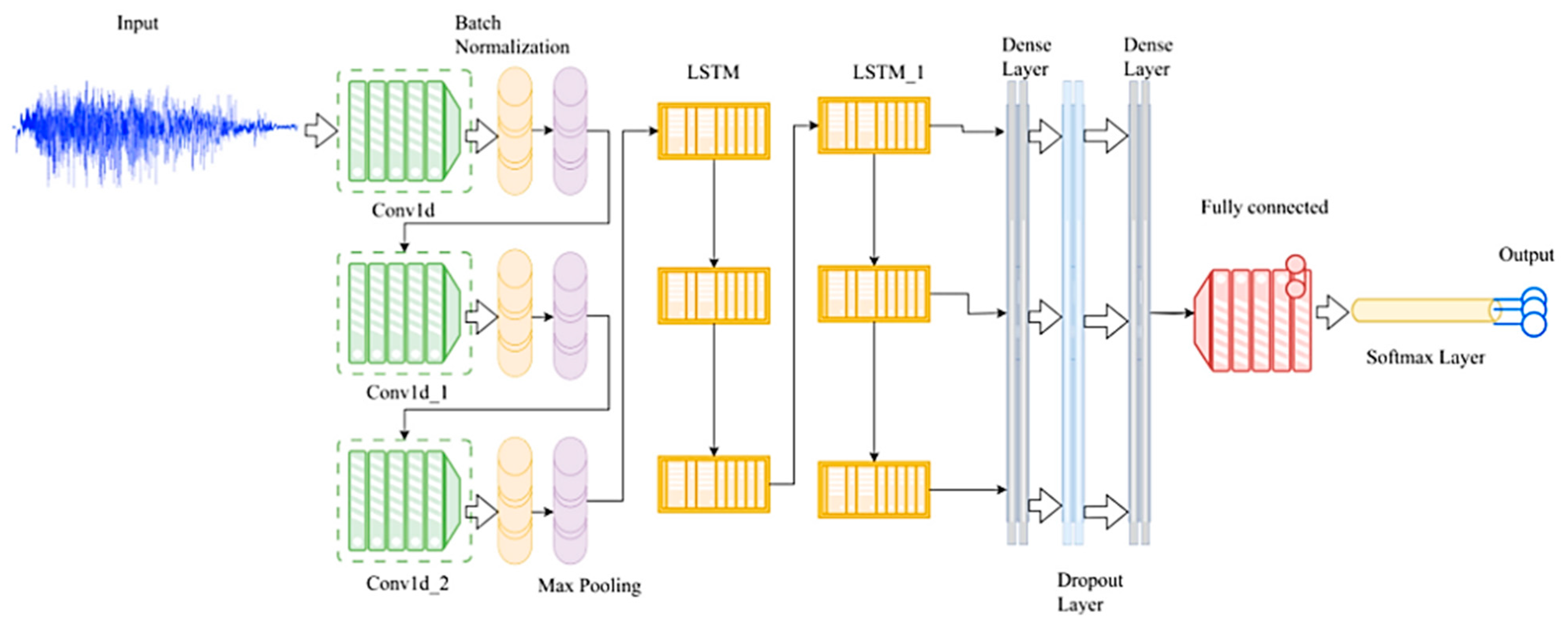
Figure 11. CNN-LSTM hybrid architecture for temporal-spatial MI decoding [56].

• Multi-Scale Hybrid Convolutional Neural Network (MSHCNN): The MSHCNN architecture shown in Figure 12 is designed to mitigate EEG non-stationarity and subject variability through a multi-scale extraction framework. The structural logic employs a Feature Enhancement stage to encode hemispheric contrast and lateralized ERD through symmetrical electrode analysis. Parallel M1DCNN and M2DCNN blocks are utilized to capture concurrent 1D temporal and 2D spatial-temporal topographical signatures. These feature maps are integrated within a Feature Splicing Block and refined through Average Pooling to manage dimensionality. The final classification path is executed through a hierarchical Output Block using ReLU-activated layers and Softmax, supported by a regularization suite of Batch Normalization, Dropout, and L2 penalties to ensure numerical stability [15].
• TSFCNN: The TSFCNet framework shown in Figure 13 utilizes a multi-domain extraction strategy to isolate temporal, spatial, and spectral features via a MixConv-Residual block and a specialized TSF-Conv block. To account for subject-specific variability, the MixConv-Residual stage incorporates mixed depthwise convolutions (kernels 15 to 125) and residual connections to stabilize gradient flow. The TSF-Conv architecture employs parallel streams to isolate specific neural domains, utilizing a variance layer in place of standard max-pooling to capture spectral power fluctuations such as ERD and ERS. The final classification logic is driven by a Softmax-activated layer and a joint loss function (Categorical Cross-Entropy and Center Loss), a strategy designed to minimize intra-class variation and reinforce decision boundary robustness [57].
• Interactive Frequency Convolutional Neural Network (IFNET): The IFNet architecture shown in Figure 14 is a specialized framework designed to decode MI by incorporating neurophysiological priors based on Cross-Frequency Coupling (CFC). The structural logic modifies the standard EEGNet design by reversing the sequence of temporal and spatial filtering, utilizing 1D point-wise convolutions to maintain a compact parameter set. Within the Spectro-Spatial Feature Representation stage, the signal is partitioned into low-frequency (4–16 Hz) and high-frequency (16–40 Hz) bands. Each band is subjected to spatial convolution followed by depthwise temporal convolution, as represented by Equation (79), with kernel sizes scaled to the specific wavelengths of mu and beta rhythms [58].

$$\begin{gathered} U_l={\widehat{F}}_t\left({\widehat{F}}_s\left(X_l\right)\right) \\ {U}_h={\tilde{F}}_t\left({\tilde{F}}_s\left(X_h\right)\right) \end{gathered}$$

(79)

In the Cross-Frequency Interactions stage, filtered bands are integrated via element-wise addition to couple multi-band features while preserving distinct characteristics through learnable affine parameters. The classification logic employs temporal average pooling over 0.5 s segments to capture dynamics and reduce dimensionality. To address subject variability and transient artifacts, the framework utilizes Repeated Trial Augmentation (random cropping and erasing) before the final dropout-regularized fully connected layer and Softmax output [58].

• Self-Supervised Contrastive Few-Shot Network: The Self-Supervised Contrastive Few-Shot Network in Figure 15 designed to address data scarcity and signal non-stationarity through an integrated SimCLR-based contrastive learning module and a Prototypical-EEGNet. The self-supervised architecture utilizes temporal TimeReverse and SignFlip data augmentation to derive feature representations, optimized via the NT-Xent (Normalized Temperature-scaled Cross-Entropy) loss to maximize similarity between augmented views of identical trials. The underlying EEGNet-based backbone employs depthwise and separable convolutions to ensure a compact parameter set. Within the classification logic, a Prototypical Network maps features into an embedding space defined by central prototype vectors. Classification is determined by the Euclidean distance between test samples and these prototypes, a strategy intended to facilitate generalization to new subjects with minimal training data. This hybrid approach acts as a mitigation strategy for the high variability and low SNR typically found in traditional supervised pipelines [59].

The evaluative audit in

Table 13. Comparative Summary of Classification Models.

Method	Robustness	Computational Complexity	Latency	Interpretability	Generalizability
LDA	Moderate	Minimal	Near Zero	High	Moderate
SVM	High	Moderate	Low	Moderate	Moderate
CNN	High	High	Moderate	Low	High
CNN-LSTM	High	Very High	Moderate	Low	High
MSHCNN	Very High	High	Moderate	Low	High
TSFCNN	High	High	Moderate	Low	High
SCFL	High	Moderate	Low	Moderate	High

(defined by the criteria in Table A2) presents the operational trade-off between algorithmic mapping power and real-time execution stability. Linear Discriminant Analysis (LDA) is characterized by a minimal computational footprint and near-zero latency, serving as a stable baseline for rapid command translation. However, the audit suggests that its linear decision boundary may be constrained when addressing the complex, non-stationary signal drifts characteristic of motor imagery. To navigate these high-dimensional feature spaces, Support Vector Machines (SVM) and optimized frameworks such as SCFL demonstrate a capacity for increased robustness without the overhead of deep architectures. While models such as MSHCNN and TSFCNN exhibit high generalizability within the audited literature, their algorithmic complexity is noted for its potential to introduce processing lag. Consequently, the analysis indicates that methods balancing moderate complexity with low latency are particularly suited for the response-time requirements of real-time control.

2.5. Performance Metrics

The evaluation of system performance is facilitated through various quantitative measures. True Positive (TP) refers to the accurate identification of a condition or trait, while False Positive (FP) relates to the incorrect identification of a condition or trait. True Negative (TN) involves the accurate identification of the absence of a condition or trait, whereas False Negative (FN) denotes the incorrect identification of the absence of a condition or trait. Based on the variables TP, TN, FP, and FN, several performance measures are defined as follows from Equation (80) to Equation (81):

Accuracy: The ratio of the sum of TP and TN to the total number of samples in a dataset is represented by Equation (80):

$$Accuracy={\displaystyle \frac{TP+TN}{TP+TN+FP+FN}}$$

(80)

F1-Score: Harmonic mean of Precision and Recall providing a balanced assessment of the model’s performance represented by Equation (81):

$$F1-score={\displaystyle \frac{2·TP}{2·TP+FN+FP}}$$

(81)

Signal-to-Noise Ratio: The ratio of signal power to noise power which affects the reliability of the signal represented by Equation (82):

$$SNR={10log}_{10}({\displaystyle \frac{{\sum }_{t=0}^{N-1}{\left[x\left(t\right)\right]}^2}{{\sum }_{t=0}^{N-1}{\left[x\left(t\right)-y\left(t\right)\right]}^2}})$$

(82)

where x(t) is the signal values of the initial EEG data, y(t) is the denoised EEG data and N is the total sample count in the EEG data.

Mean Squared Error (MSE): Average squared error between original signal and reconstructed signal. It is a measure of signal fidelity and provides the amount of distortion between the signals represented by Equation (83).

$$MSE={\displaystyle \frac{1}{N}}{\displaystyle \sum _{t=0}^{N-1}}{[x\left(t\right)-y\left(t\right)]}^2$$

(83)

Cohens Kappa: Quantified by the percentage agreement between the actual experimental trials and the estimated labels produced by the classification output represented by Equation (84):

$$k={\displaystyle \frac{P_o-P_c}{1-P_c}}$$

(84)

where $P_o$ is relative observed agreement and $P_c$ is the hypothetical probability of chance agreement.

3. Results

3.1. Signal Preprocessing Results

To validate the mathematical principles discussed in this review, a quantitative case study was performed using experimental data derived from [30]. The evaluation of Subject 1 and Subject 2 highlights the impact of different IIR filter configurations on signal quality shown in Figure 16. The baseline noisy signal recorded an SNR of 43.180 dB for Subject 1, which had a marginal increase to 43.190 dB with the Bandstop filter and a peak of 43.327 dB with the Low Pass filter. A stronger baseline at 44.764 dB for Subject 2, which improved to 44.828 dB after Bandstop filtering and reached 44.987 dB with the Low-Pass filter. Evaluating the reconstruction loss, the Mean Squared Error (MSE) for both subjects started at 0.0099. The Bandstop filter effectively reduced this loss to 0.0095 for Subject 2, while the Low Pass filter further reduced it to 0.0090. In contrast, Subject 1’s MSE remained stagnant at 0.0099 after the Bandstop filter, only dropping to 0.0095 with the Low-Pass application. The Root Mean Square Error (RMSE) follows a similar trend, remaining consistently below 0.1 for both subjects across all filter types. These results suggest while both filters contribute to signal enhancement, the Low Pass IIR filter provides a more substantial reduction in reconstruction loss and a higher boost in SNR than the Bandstop filter for both individuals.

To evaluate the mathematical impact of filter order on signal quality, a quantitative case study was performed using an FIR Low Pass filter with 4 window techniques applied to Subject 1 and Subject 2. Figure 17 shows the impact of filter order on signal quality using a Hanning Window. The baseline SNR (prior to filtering) was recorded at 43.06 dB and reaches a maximum of 47.72 dB at Order 4 for Subject 1, before beginning a steady decline as the order increases further. A similar trend is observed in Subject 2 but achieves a higher peak SNR of 48.64 dB at Order 3. It is important to note that certain filter orders, specifically Order 2 and Order 7, were omitted in the source study; as a result, these points are excluded from the current analysis. The reconstruction loss, measured through Mean Squared Error (MSE), provides further mathematical insight into filter optimization. At Order 0, both subjects show their highest reconstruction loss, with values at or above 0.010. As the filter order increases to Order 4, the MSE for Subject 1 drops to its lowest point of 0.0035, while Subject 2 reaches its minimum of 0.0037 at Order 3. However, beyond these points, the MSE begins to rise again, most notably for Subject 2, where the error increases back to 0.0091 by Order 8. These results conclude that increasing the filter order only improves signal quality up to a specific mathematical threshold; exceeding this order introduces unnecessary complexity and reconstruction error, which is particularly detrimental for maintaining low-latency performance in a BCI pipeline.

Figure 18 shows the impact of filter order using an FIR Low Pass filter with a Hamming window applied to Subject 1 and Subject 2. The SNR baseline of 43.06 dB at Order 0 increases to a maximum of 47.63 dB at Order 6 for Subject 1. Subject 2 follows a similar trend, starting at 44.72 dB and reaching a peak SNR of 49.18 dB at Order 6. It is important to note that certain filter orders, specifically Order 2 and Order 3, were omitted in the source study; as a result, these points are excluded from the current analysis.

The reconstruction loss, measured through Mean Squared Error (MSE), provides further mathematical insight into the optimization of the Hamming window. At Order 0, both subjects show their highest reconstruction loss, with values reaching the 0.010 threshold. As the filter order increases, the MSE for both subjects drops significantly and stabilizes. Subject 1 reaches a minimum MSE of 0.0035 at Order 6, while Subject 2 achieves its lowest error of 0.0036 at the same order. Unlike the Hanning window results, the Hamming window maintains a relatively stable and low MSE even as the order reaches 8, though a slight upward trend in error is observed after the Order 6 peak. These results conclude that for a Hamming-based FIR Low Pass filter, Order 6 represents the optimal spot for maximizing signal-to-noise ratio while minimizing reconstruction loss, providing a stable foundation for a low-latency pipeline.

Figure 19 shows the impact of filter order using an FIR Low Pass filter with a Blackman window applied to Subject 1 and Subject 2. The SNR starts at 43.06 dB at Order 0, remains nearly identical at Order 4, and then increases to a peak of 47.67 dB at Order 6 for Subject 1. Subject 2 shows a more significant jump, starting at 44.72 dB and reaching its maximum SNR of 49.10 dB at Order 5. It is important to note that several filter orders, specifically Orders 1, 2, and 3, were omitted in the source study; as a result, these points are excluded from the current analysis. The reconstruction loss, measured through Mean Squared Error (MSE), reveals a distinct behavior for the Blackman window compared to previous methods. At Order 0 and Order 4, the MSE for both subjects remains high, hitting the 0.010 threshold. However, a sharp shift occurs at Order 5, where the MSE for both subjects drops abruptly to approximately 0.0036. Subject 1 achieves its absolute minimum error of 0.0035 at Order 6, while Subject 2 maintains a stable error of 0.0037 from Order 6 through Order 8. These results conclude that for a Blackman-based FIR Low Pass filter, any order below 5 is insufficient for noise reduction, with Order 6 providing the most consistent balance of high SNR and low reconstruction loss across both subjects.

Figure 20 shows the impact of filter order using an FIR Low Pass filter with a Kaiser window applied to Subject 1 and Subject 2. The SNR baseline of 43.06 dB at Order 0 increases to a peak of 48.40 dB at Order 4, followed by a sharp reduction as the order progresses to 8 for Subject 1. Subject 2 exhibits its maximum performance earlier, reaching a peak SNR of 49.72 dB at Order 3 before a similar decline occurs. Consistent with previous observations, data for certain configurations, specifically Order 2 and Order 7, were not used in the source study and are therefore absent from the analysis. The reconstruction loss, measured through Mean Squared Error (MSE), provides a clear justification for these optimal points. At Order 0, both subjects record their maximum MSE near 0.010. The error reaches a minimum of 0.0029 at Order 4, aligning perfectly with its peak SNR Subject 1. Subject 2 achieves its lowest reconstruction loss of 0.0035 at Order 3. Notably, as the filter order increases beyond these specific values, the MSE increases significantly, nearly returning to baseline levels by Order 8 for both subjects. These results suggest for a Kaiser-windowed FIR filter, the mathematical sweet spot is restricted to a very narrow range of low filter orders, as higher orders introduce substantial reconstruction error that would compromise signal fidelity in a pipeline.

3.2. BSS and Decomposition

To validate the real-world efficiency of the preprocessing stage independently of the primary experimental subjects [16], a computational benchmark was performed across 158 distinct datasets within a source study as shown in Figure 21. This large-scale analysis provides a generalized mathematical proof for the benefits of Riemannian manifold mapping in EEG cleaning, comparing standard Artifact Subspace Reconstruction (ASR) against the more efficient rASR variant. The results from that study demonstrate that standard ASR recorded a mean execution time of 10 s, while rASR significantly reduced the computational demand to a mean of 5.6 s. By nearly halving the execution time and narrowing the variance, the study’s findings prove rASR to be mathematically more stable for high-throughput data processing.

In the context of a MI-BCI system, this independent benchmark of 158 datasets highlights the expensive temporal cost of high-dimensional processing. Using rASR as the engine for artifact rejection ensures the system can maintain the low-latency response required for a pipeline without the accumulation of signal lag that typically plagues complex EEG environments.

A comparative analysis of the classification performance across standalone and hybrid architectures, specifically PCA [47], VMD [60], WT-AR [45], DWT-EMD [61], and ICA-WT [13], reveals a correlation between mathematical synergy and decoding accuracy as shown in Figure 22. While these studies use heterogeneous datasets, the synthesis focuses on identifying architectural behavior patterns to isolate how specific mathematical frameworks manage signal complexity independently of dataset-specific bias. The comparative analysis reveals while standalone benchmarks like PCA (75.00%) and VMD (68.20%) struggle with the complex noise floor of EEG signals, hybrid architectures enhance classification accuracy. The WT-AR (LDA) framework reaches 92.10%, proving that multi-resolution decomposition effectively linearizes the feature manifold. However, the DWT-EMD (95.10%) hybrid delivers the highest performance by using SVM to map non-linear entropy features, effectively mitigating EMD’s mode-mixing issues. In contrast, the lower results of ICA-WT (78.41%) suggest that without specific sub-band refinement, spatial-frequency hybrids may still be limited by residual noise. These results suggest BCI reliability is driven by the optimization of the decomposition stage, which reduces the computational overhead on the classifier used.

3.3. Feature Extraction Results

The results illustrated in Figure 23, which were obtained from a conducted study [12], demonstrate a clear divergence in classification performance when using a Linear Discriminant Analysis (LDA) classifier across a five-subject pool. The combination of Autoregressive (AR) modeling and LDA provides the superior mathematical representation, reaching an accuracy of 74.2% for Subject 1. In contrast, Subject 2 achieves their peak performance of 73.4% in the by incorporating Moving Average Model features into the LDA classifier, indicating a preference for smoothed temporal data. A significant shift is observed for Subjects 3 and 4, where Alpha-BP-PSD features emerge as the most effective input for the classifier, yielding accuracies of 74.6% and 75.7% respectively. This suggests that for these individuals, the power distribution within the alpha frequency band is more discriminative for the LDA decision boundary than time-domain modeling. Finally, Subject 5 displays more balanced results within the study, with the Alpha-BP-PSD and LDA pairing maintaining a lead at 67.3%. Collectively, these crossovers, where the winning feature extraction method fluctuates while the LDA classifier remains constant, suggest the optimal feature manifold is highly subject dependent.

3.4. Feature Selection Results

To evaluate the mathematical efficiency of dimensionality reduction within the signal processing pipeline, seven feature selection algorithms were benchmarked across five subjects from the BCI Competition III Dataset 4A using both SVM and LDA classifiers from independent studies [3,18,19]. In the SVM environment shown in Figure 24a, Neighborhood Component Analysis (NCA) emerged as the superior approach, achieving a peak classification accuracy of 98.9% for Subject al and 98.2% for Subject aw, while maintaining a robust 76.7% even for the lower-performing Subject av. The LDA results mirror these high-performance trends, with NCA maintaining a slight lead for Subject av at 76.1%. However, in Figure 24b, the Relief-F algorithm demonstrated computational efficiency with the LDA classifier, reaching a peak of 97.8% for Subject aw and providing a substantial boost for Subject av to 75.6%, which outperforms the 70.0% mRMR baseline. While NCA technically holds the accuracy lead for Subject av by a 0.5% margin, the distance-based logic of Relief-F proves to be a highly competitive alternative for linear classification. These findings suggest that while gradient-based optimization in NCA is ideal for non-linear SVM classification, Relief-F offers a mathematically efficient and stable alternative that is particularly suited for maintaining high accuracy within the low-latency constraints of a BCI pipeline.

To evaluate the computational efficiency and feasibility for a BCI pipeline, the execution time for each feature selection algorithm was measured in seconds. A significant mathematical disparity is observed between Subject aa and the rest of the unit. For Subject aa, computational costs are notably higher across all algorithms. In the SVM environment shown in Figure 25a, Relief-F required 0.51 s, while in the LDA environment, as shown in Figure 25b, FSV peaked at 0.38 s. In contrast, for subjects al, av, aw, and ay, the computational overhead remains negligible, consistently hovering around 0.01 to 0.02 s regardless of the classifier or algorithm used. Notably, the data for Neighborhood Component Analysis (NCA) is marked as N.A. across all subjects in both timing plots, indicating this specific metric was not used or recorded within the source study. Documenting this absence is essential for the integrity of the review, as it highlights a gap in the available literature regarding the real-time trade-off for NCA. While NCA provides superior accuracy reaching 98.9% for Subject al, the lack of recorded timing data means its impact on processing lag cannot be confirmed. For high-demand subjects like aa, mRMR remains the most efficient recorded option at 0.16 s, though it sacrifices accuracy to achieve this speed. These results suggest that for most subjects, the mathematical cost of feature selection supports real-time use, but the choice of algorithm must remain sensitive to the specific subject’s data complexity and the known limits of the source study.

The inclusion of a Without Feature Selection baseline [7] in Figure 26 provides a contrast to the optimized algorithms, revealing that for some subjects, the full dimensionality of the extracted data maximizes classification accuracy. For Subject aw, the absence of feature selection yielded the study’s peak accuracy of 99.6%. For Subject av, it reached 88.9%, which represents the highest accuracy recorded for that specific subject across all tests. However, the marginal accuracy gains for other subjects, such as the 98.6% baseline for Subject al compared to the 98.7% achieved by Relief-F suggest that a high percentage of the original features are redundant.

In the context of a low-latency pipeline, these results highlight a trade-off. While the specific feature count for the baseline was not explicitly recorded in the study [7], it represents the raw, high-dimensional space before any pruning occurred. The fact that algorithms such as Relief-F and NCA can approach or even match these baseline figures while operating on a reduced feature matrix is the true success of the pipeline. This highlights the use of feature selection not merely to improve scores but to achieve a mathematically sparse representation of the signal that is compatible with real-time processing.

3.5. Classification Results

Table 14. Exploration of LDA Classifier Performance: Impact of Disclosed vs. Opaque Hyperparameter Configurations.

Paper	Year	Hyperparameter	Accuracy	Notes
[3]	2020	None Specified	90.07%	High performance is reported but lacks the deterministic constants required for verification.
[62]	2021	Parameter Solver—‘lsqr’ Shrinkage—0.81	87.61%	Full disclosure of shrinkage allows for stable implementation in portable BCI systems.
[63]	2024	Default Settings	64.15%	Demonstrates a ~23% performance drop when relying on standard settings without fine tuning.

reveals an implementation gap that directly compares reporting transparency with system reliability. While [3] reports a high accuracy of 90.07%, its “None Specified” status creates a reproducibility gap, as the absence of model parameters prevents the results from being verified. In contrast, the study [62] demonstrates by disclosing specific parameters, it provides the stable mathematical framework required for replication despite a lower accuracy of 87.61%. The baseline in [63] serves as proof of the default settings, where a failure to perform fine-tuning resulted in an approximately 23% performance drop (64.15%). This confirms hyperparameter optimization is an important requirement for functional, high-performance MI systems.

The synthesis of Support Vector Machine (SVM) configurations in

Table 15. Exploration of SVM Classifier Performance: Impact of Disclosed vs. Opaque Hyperparameter Configurations.

Paper	Year	Hyperparameter	Accuracy	Notes
[64]	2018	Radial Basis Function C and Gamma (γ)—automatic optimized Population size = 5	86.6%	While parameters are automatically optimized the failure to report the resulting constants prevents replication of model.
[3]	2020	None Specified	90.00%	Reports high accuracy but omits the kernel penalty (C) and scale (gamma), preventing hardware replication
[65]	2024	C—2 Gamma (γ)—0.35 Radial Basis Function	95.37%	Disclosure of specific constants allows for immediate firmware parameterization in portable BC

reveals a systemic Parametric Opacity that compromises the transition from research to verified application. While study [3] reports a high accuracy of 90.00%, the omission of the kernel penalty (C) and scale creates a black-box effect that cannot be validated. In contrast, in [64], which relied on automatic optimization without reporting final constants, resulted in a lower accuracy of 86.6%, suggesting that automated tuning without transparent oversight may fail to capture the subtle neural biomarkers required for stable control. Furthermore, in study [65] establishes a reporting benchmark by disclosing specific constants alongside a peak accuracy of 95.37%. This disclosure highlights replication as it provides the specific constants observed to be effective for reconstruction in independent studies This suggests that explicit hyperparameter disclosure is not merely a reporting preference but a requirement for replication and the development of reliable assistive technology.

A focused comparison was conducted between two studies [14,17] employing self-generated datasets to evaluate the efficacy of different deep learning architectures MI decoding. As shown in Figure 27, the standalone CNN model produced a mean classification accuracy of 69.42%. In contrast, the CNN-LSTM architecture demonstrated a substantial performance gain with an offline average of 87.20%. This 17.78% difference between the two studies highlights the advantage of incorporating recurrent temporal layers. While the convolutional layers in both studies address spatial filtering, the superior results in the CNN-LSTM framework suggest that capturing the sequential dependencies of the EEG signal is important for achieving the high-accuracy thresholds required for reliable BCI control.

The analysis of classification performance shown in Figure 28 across the nine subjects from independent studies [15,57,58,59] using BCI Competition IV Dataset 2A and 2B (S1–S9) shows a high degree of intra-subject variability, highlighting the mathematical challenge of decoding non-stationary EEG manifolds. While these individual results are derived from heterogeneous subject data, the synthesis identifies distinct architectural behavior patterns to isolate how specific frameworks manage intra-subject noise independently of individual neural signatures. The MSHCNN and TSFCNet architectures emerge as the most stable performers across the unit; MSHCNN consistently achieves high results such as 98.0% for subject S4 and exceeds 90% for subjects S5 and S8, while TSFCNet peaks at 97.5% for S4. In contrast, the IFNet model exhibits instability; while it provides a localized peak for subject S3 (91.8%), it suffers from performance collapses in subjects S2 (56.4%) and S6 (60.4%), effectively dropping to near-chance levels. Notably, the SCFL model consistently registers the lowest benchmarks across the subjects, reaching a minimum of 53.7% in subject S2. Subject S3 remains an outlier for the primary models, as the performance of the MSHCNN (66.0%) fluctuates compared to its performance in other subjects, indicating a lower signal-to-noise ratio (SNR) or higher neural complexity for this individual. The presence of these outliers, combined with the behavioral discrepancies seen across self-generated data, justifies the implementation of a pipeline that carries offline parameters into online execution to ensure subject-specific stability.

The performance data from the reviewed literature is divided into two categories to ensure a methodologically fair comparison. Table 15 focuses on studies using standardized, public benchmark datasets, while

Table 16. Performance Synthesis of MI-BCI Datasets, Classifiers, and Statistical Validation.

Paper	Year	Dataset	Task (Classes)	Classifier	Average F1-Score	Average Kappa	Statistical Validation	Average Accuracy
[3]	2020	BCI Comp III 4A BCI Comp IV 2B	2 classes	SVM LDA	None Specified	None Specified	Friedmans one-way ANOVA test (p < 0.006) Turkey-Kramer post hoc (p < 0.002)	92.20% 91.36% 81.52%
[13]	2021	Physionet	None Specified	SVM LDA	None Specified	None Specified	None Specified	81.75% 78.41%
[15]	2023	BCI Comp IV 2A BCI Comp IV 2B	4 classes 2 classes	MSHCNN	None Specified	None Specified	Wiconxon signed rank test; Cohens d-value (p < 0.05; 0.825)	84.86% 85.25%
[19]	2023	BCI Comp III 4A BCI Comp III 3B	2 classes	LDA SVM	0.8935 * 0.8853 * 0.6718 * 0.6633 *	None Specified	None Specified	90.05%
[7]	2023	BCI Comp IV 1 BCI Comp III 4A	2 classes	SVM LDA	None Specified	None Specified	None Specified	90.42% 95.42%
[18]	2024	BCI Comp III 4A BCI Comp III 3B BCI Comp III 3A	2 classes 2 classes 4 classes	LDA SVM	0.8965 * 0.7435 * 0.8831 * 0.7123 *	None Specified	None Specified	91.432% 76.111%

*: manually calculated the average Kappa coefficients and F1-Scores.

examines exploratory studies using self-generated or laboratory-acquired data.

The comparative results in Table 16 highlight a relationship between Task Complexity and algorithmic success. While studies using public benchmarks consistently achieve accuracies above 90% in binary (2-class) settings, a distinct dimensionality constraint appears as the classes increase. For instance, the transition to 4-class tasks in [18] results in a performance drop from 91.43% to 76.11%, highlighting that current frameworks struggle to maintain precision in higher dimensions. While [18] experienced a performance drop in multiclass settings, Study [15] maintains a high accuracy of 84.86% on a 4-class task using a Multi-Scale Hybrid Convolutional Neural Network (MSHCNN). This outlier is significant as it suggests while linear classifiers (LDA/SVM) hit a dimensionality constraint at 4 classes, deep learning architectures can overcome this barrier. However, despite this success, the study lacks Kappa or F1-Score reporting, which prevents a full understanding of how the model manages class-specific confusion, a common issue in 4-class motor imagery.

Beyond raw percentages, the table highlights a systemic reporting gap regarding statistical validation. Despite high accuracy trends, there is a noticeable lack of formal Statistical Validation in many studies, making it difficult to verify if improvements are true breakthroughs or merely subject-specific variances. Where literature provided raw subject-specific data but omitted summary statistics, this paper manually calculated the average F1-Scores denoted by a (*). This synthesis exposes the limitations of relying solely on average accuracy, which often obscures the impact of class imbalances and signal noise. While high-order architectures such as the CNN-LSTM in [17] show promise for multiclass robustness, the frequent omission of core parameters often labeled as Not Reported remains a barrier to reproducibility. This multi-metric evaluation moves beyond a simple list of results to provide a high-fidelity map of the technical gaps that must be addressed to transition BCI models from offline benchmarks to reliable, real-time applications.

The evaluation of studies utilizing self-generated or internal laboratory data reveals a significantly higher degree of reporting variance compared to benchmark-driven literature. As shown in

Table 17. Performance Synthesis of Self-Generated Data, Classifiers, and Statistical Validation.

Paper	Year	Dataset	Task (Classes)	Classifier	Average F1-Score	Average Kappa	Statistical Validation	Average Accuracy
[12]	2015	Self-Generated	3 classes	LDA	None Specified	None Specified	None Specified	MAV- 68.5% AR—68.4% $\alpha$-BP-PSD—71.8% $\alpha$-BP-PSD—70.1%
[16]	2019	Self-Generated	None Specified	None Specified	None Specified	None Specified	Repeated-measures ANOVA, paired t-test	None Specified
[14]	2022	Self-Generated	2 classes	CSP-LDA CNN	Left Hand (0.5293) Right Hand (0.5183) Left Hand (0.6907) Right Hand (0.6859)	None Specified	Shapiro–Wilk normality test: CSP + LDA (W = 0.97, p = 0.12), CNN (W = 0.98, p = 0.66) pairwise t-test (t(53) = 22.12, p < 0.001)	69.42% 52.56%
[17]	2024	Self-Generated	7 classes	CNN-LSTM	Not Specified	0.9289	None Specified	Offline—87.20% Online—93.12%

, these papers often focus on specific, real-world operational environments; however, it highlights a complexity gap where the number of MI tasks (classes) directly dictates the choice of classifier. While binary tasks in [14] use standard CSP-LDA and CNN approaches to achieve stable results, the transition to high-dimensionality control, the 7-class task in [17], requires the integration of CNN-LSTM architectures to manage the increased temporal and spatial data load.

A primary observation in this subset is the contrast in methodological disclosure. For instance, study [14] provides a rigorous mathematical audit, employing a Shapiro–Wilk normality test and a pairwise t-test to validate the statistical significance of the reported results. This level of transparency represents a professional standard for BCI research, allowing for a clear verification of the system’s stability. In contrast, studies such as [12] and [16] rely almost exclusively on raw accuracy percentages without providing secondary metrics like Kappa or F1-Scores, which are important for understanding how a model handles the confusion between 3 or more classes.

The reliance on isolated accuracy metrics in these laboratory settings highlights a significant Black Box risk. Without standardized datasets or statistical validation, it becomes difficult to determine if high performance such as the 93.12% online accuracy in [17] is a result of algorithmic robustness, specific environmental conditions, or subject-specific variance. The classification of 7 classes in [17] suggests deep learning is effective for complex, self-generated data, yet the frequent omission of core parameters/metrics remains a barrier to cross-study validation.

4. Discussion

The following discussion is structured as a targeted technical audit of ten intentionally selected MI-BCI studies. The primary audited sample revealed a high concentration of Common Spatial Pattern (CSP) and Deep Learning architectures yet exhibited a notable absence of artifact removal stages such as Blind Source Separation (BSS) and current Deep Learning architectures. To address this gap and provide a robust landscape, secondary literature is utilized as a theoretical benchmark. This selective review design prioritizes high-granularity evaluation over broad survey volume; therefore, the subsequent comparisons are presented as descriptive trends within the audited sample rather than generalized claims of universal method superiority across the broader MI-BCI field.

4.1. Audit of Signal Integrity and Preprocessing Trends

The comparative analysis of filter architectures suggests a trade-off between attenuation depth and reconstruction fidelity. Data indicates a trend that broad-spectrum Low Pass configurations appear more effective than targeted Bandstop filters, as the latter often reach an MSE value that leaves signal residuals stagnant. A peak and decline trend observed in Kaiser and Hanning windows is interpreted as a theoretical upper bound. Increasing the filter order beyond a specific threshold introduces phase-response distortions and reconstruction errors that compromise the pipeline. In contrast, the Hamming and Blackman windows exhibit a stability trend, with Order 6 representing an optimal value for consistent signal integrity. While the Blackman window requires higher complexity to overcome noise thresholds, the Hamming window provides a consistent framework, ensuring signal stability without the sensitivity to order progression found in the Kaiser architecture. This stability is beneficial for preventing propagated errors in subsequent feature extraction stages. The evaluation of the audited sample suggests the primary advantage of hybrid systems, specifically the DWT-EMD framework, is associated with the ability to linearize the feature manifold and mitigate mode mixing. In the reviewed literature, this pre-refinement stage appeared to reduce the burden on the classifier; this is attributed to decreasing feature space entropy, potentially allowing for more stable decoding. In contrast, while standalone frameworks such as PCA and VMD were observed to report lower relative accuracies within the audited sample, these results interpreted as a descriptive trend within the context of the specific noise floors and experimental conditions of those datasets. Furthermore, while ICA-based hybrids demonstrated improved spatial separation, their constraints regarding non-stationarity may limit their stability compared to temporal-spectral hybrids such as DWT-EMD. These results suggest that the decomposition stage is a significant driver of BCI reliability; however, the extent of this impact remains a descriptive trend observed across the audited architectures.

4.2. Challenges in Computational Portability and Real-Time Suitability

The benchmarking of multi-subject datasets supports the trend for the transition from standard Artifact Subspace Reconstruction (ASR) to the Riemannian-based rASR variant. An observed benefit of rASR lies in its ability to reduce average execution time while simultaneously lowering computational variance. From a mathematical perspective, this stability is critical for high-throughput data streams, as it minimizes the overhead per data block and prevents the accumulation of signal lag. In contrast, the results suggest the standard ASR presents a higher temporal cost. Its high computational demand and wider variance introduce a level of complexity less suitable for real-time feedback loops, where unpredictable processing spikes can disrupt system continuity. Even with the improvements offered by rASR, the results highlight that high-dimensional EEG cleaning remains a resource-intensive task. As a result, Riemannian optimization appears critical for maintaining causal integrity, ensuring the preprocessing stage does not induce the signal buffering typically associated with standard ASR implementations in deterministic environments.

The evaluation of feature selection algorithms within the audited sample reveals a difference between classification optimization and computational overhead. In the reviewed literature, gradient-based Neighborhood Component Analysis (NCA) was observed to report high static accuracy metrics; however, the omission of execution metrics for NCA invalidates its claims of real-time superiority, as the potential for indeterminate lag remains unquantified. This lack of reporting introduces a risk of indeterminate lag when compared to more transparently documented frameworks. In contrast, Relief-F demonstrated a more balanced profile within the audited cases, appearing to maintain signal fidelity with minimal reported processing requirements. An observation in this synthesis is the subject-dependent nature of computational cost. The variability in processing times across different subject profiles suggests that fixed algorithms may face challenges in maintaining temporal integrity as data complexity scales. Furthermore, while methods such as mRMR exhibited lower peak accuracies relative to NCA in these instances, they offered a more documented temporal footprint. These findings suggest that within the context of the audited environments, prioritizing documented efficiency and temporal predictability may be as critical as isolated accuracy metrics for ensuring feedback loop continuity.

Within the audited sample, the transition from standalone convolutional architectures to hybrid CNN-LSTM frameworks reveals a trade-off between structural complexity and decoding reliability. The primary advantage of this hybrid approach, as observed in the surveyed literature, lies in its temporal feature extraction. By integrating recurrent layers, these models appear to move beyond static spatial snapshots to capture sequential dependencies. However, these benefits introduce computational latency, as the increased parameter count can strain the temporal integrity of a pipeline. By decomposing standard convolutions into depthwise and pointwise operations, certain surveyed architectures utilize SCFL to maintain high-fidelity feature maps while reducing the trainable parameter count. Furthermore, a comparative audit of multi-scale architectures such as MSHCNN, TSFCNet, and IFNet highlights the challenge of intra-subject variability across diverse datasets. While multi-scale convolutional layers are effective at isolating invariant spatial features, certain audited architectures exhibit performance collapses when faced with low SNR outliers.

4.3. Subject-Dependent Variability and Task Dimensionality

The observed variability across subjects supports the implementation of a multi-feature extraction layer. By acknowledging that individual neural profiles often require distinct mathematical manifolds, such as a preference for Autoregressive (AR) modeling in certain subjects versus Power Spectral Density (PSD) in others, the pipeline can achieve higher peak accuracies than a rigid, single-method architecture. This adaptive flexibility is intended to allow the LDA classifier to operate on the most separable data possible, which is critical for maintaining robust performance in practical applications. However, the disadvantage of this subject-dependent performance is the requisite complexity of the feature selection stage. As no single extraction method is universally superior, the system typically requires incorporating an intelligent ranking mechanism to identify optimal features for each user. This requirement introduces an additional layer of processing and requires a calibration phase. Furthermore, while focusing on a singular extraction type per subject maintains computational efficiency and low-latency integrity, it may be less suitable for capturing the multi-domain signatures often observed in high-complexity neural profiles.

Within the audited sample, the inclusion of a baseline model without feature selection serves as a benchmark for classification potential, highlighting that raw, high-dimensional feature spaces may contain subtle discriminative information that certain algorithms risk discarding. However, the reviewed literature indicates that maintaining this full dimensionality introduces redundancy, where a substantial portion of the original feature set contributes to the noise floor rather than the signal. From a structural perspective, these high-dimensional spaces represent a documented temporal risk in sequential processing environments. The primary success observed in the integrated pipelines of the 10 studies lies in the ability of algorithms such as Relief-F and NCA to approximate these baseline accuracy figures while operating on a sparse feature matrix. In the context of these audited architectures, this supports the role of feature selection as a functional necessity, achieving competitive performance while ensuring the architecture remains computationally lean. By reducing the feature dimension, the surveyed systems appear to avoid the latent processing lag associated with raw EEG data, maintaining the deterministic integrity required for functional, low-latency control within those specific experimental conditions.

An analysis of the reviewed literature indicates an inverse correlation between task dimensionality and classification reliability. While binary paradigms consistently achieve performance benchmarks above 90%, the transition to multi-class environments results in an accuracy decline, with reported figures dropping to the 52–87% range. This performance decay suggests that higher task complexity introduces significant spectral and spatial overlap, which complicates the feature separation process and strains the discriminatory capacity of the classifier. Despite these performance trends, a research gap persists regarding the statistical rigor of the sampled studies. Several studies reporting accuracy fail to include validation metrics such as F1-scores, Cohen’s Kappa, or formal significance testing (e.g., ANOVA/Wilcoxon). The absence of F1-scores and Kappa coefficients obscures the model’s true discriminatory power, rendering reported accuracies vulnerable to class imbalance artifacts. Without these metrics, it remains ambiguous whether the recorded successes are due to a robust architectural manifold or are merely localized artifacts of specific subject profiles. The scarcity of cross-subject validation and rigorous statistical depth makes it impossible to conclude if these pipelines can maintain deterministic integrity in real-time, practical applications.

4.4. BCI Applications

This paper focuses exclusively on endogenous BCI systems, which provide maximum independence by relying on the user’s internal intent rather than external stimuli. By focusing on Motor Imagery, these systems allow individuals with severe disabilities to initiate commands voluntarily. This means the technology waits for the user’s thoughts instead of requiring a computer prompt. This lens of personal control is used to categorize the reviewed literature into industries aimed at bridging the gap between internal neural signals and physical environmental interaction.

4.4.1. Restorative Applications and Digital Autonomy

In the biomedical sector, endogenous BCIs focus on restorative technologies that translate neural intent into physical action for individuals with severe disabilities. A primary application is the control of screen cursors, an area active for over thirty years but still plagued by a lack of operational smoothness. While modern literature reports classification accuracies exceeding 90%, these results are often achieved through highly personalized models requiring extensive calibration. This reliance on individual-specific tuning, combined with high hardware costs, remains a major barrier to a generalized mathematical framework and broad clinical adoption [66].

4.4.2. Physiological Complexity in Neural Prosthetics

The development of BCI-driven prosthetics aims to restore motor function by mapping neural intent to robotic actuators, a task that requires translating complex brain patterns into numerous discrete motor commands [67,68]. To address the limitations of EEG alone, researchers often employ multimodal approaches such as integrating Electromyogram (EMG), yet practical implementation remains narrow. A significant gap exists between laboratory success and real-world viability. While papers frequently report high classification accuracy, it often omits critical data on power consumption and processing constraints. As a result, current systems lack the fluid, multi-tasking capabilities of natural limbs and struggle to operate effectively within the strict hardware limitations of non-laboratory environments [66].

4.4.3. Risk Assessment in Brain-Driven Mobility

Research into smart wheelchairs driven by endogenous brain signals is an important intervention for individuals with Motor Neuron Disease (MND), Spinal Cord Injury (SCI) or stroke. Patients with conditions such as Amyotrophic Lateral Sclerosis (ALS), who retain cognitive function despite losing muscle control, are uniquely suited for motor-imagery control. However, mobility applications face higher risks than other BCI sectors. A command error or processing delay might be a minor inconvenience in a computer task resulting in a physical injury in a navigation context. Safe navigation requires precise, time-sensitive execution in dynamic, ever-changing environments. The transition of these wheelchairs from experimental prototypes to clinical tools depends on robustness and low-latency response metrics that are often overlooked in current studies that prioritize raw accuracy over real-world safety and environmental adaptability [66,69,70].

4.5. Limitations

The primary limitation of this study is the constrained sample size of the reviewed literature, which is restricted to the 10 representative high-density papers synthesized in the preceding tables. While this small sample was necessary to facilitate a forensic mathematical audit of governing equations, it inherently introduces a selection bias toward studies with higher levels of technical disclosure. A larger, more diverse sample size might have provided a more statistically significant map of the field, potentially revealing whether the identified gap is isolated to these specific high-performing frameworks or are systemic across the broader BCI community.

5. Conclusions

This paper conducted a targeted technical audit of ten selected high-density MI-BCI pipelines to evaluate the alignment between reported performance and practical engineering suitability. Rather than providing a broad survey, this investigation performed a deep-dive analysis of these specific architectures to identify the Parametric Opacity that often hinders reproducibility. The results demonstrate that while reported offline accuracies in these sampled studies reach as high as 95.42%, the lack of granular reporting regarding filter orders and causal constraints makes these benchmarks difficult to translate into real-time environments.

The audit specifically evaluated the trade-offs between standalone and hybrid architectures, finding that while hybrid configurations often enhance noise-rejection, they frequently introduce undocumented computational overhead. Furthermore, while the audit identifies Neighborhood Component Analysis (NCA) as a stable feature selection algorithm, the systemic absence of reported execution times remains a primary barrier to verifying its viability. These reporting gaps suggest that the current focus on peak accuracy often comes at the cost of the deterministic transparency required for reliable assistive technology.

Although the audited pipelines which encompass both traditional and deep learning models demonstrate high performance in subject-specific contexts, inter-session and inter-subject variation pose severe implications for practical BCI classification. The observed decline in performance across individual subjects is attributed to the stochastic nature of EEG neural dynamics found within the sampled literature. Consequently, future work will explore the applicability of domain adaptation and domain selection algorithms, coupled with SHAP (SHapley Additive exPlanations) analysis, to address these dynamics and enhance cross-subject classification.

References

1. Mdluli, B.; Khumalo, P.; Maswanganyi, R.C. Signal Preprocessing, Decomposition and Feature Extraction Methods in EEG-Based BCIs. Appl. Sci. 2025, 15, 12075. [Google Scholar] [CrossRef]
2. Nicolas-Alonso, L.F.; Gomez-Gil, J. Brain computer interfaces, a review. Sensors 2012, 12, 1211–1279. [Google Scholar] [CrossRef]
3. Molla, M.K.I.; Al Shiam, A.; Islam, M.R.; Tanaka, T. Discriminative Feature Selection-Based Motor Imagery Classification Using EEG Signal. IEEE Access 2020, 8, 98255–98265. [Google Scholar] [CrossRef]
4. Padfield, N.; Zabalza, J.; Zhao, H.; Masero, V.; Ren, J. EEG-based brain-computer interfaces using motor-imagery: Techniques and challenges. Sensors 2019, 19, 1423. [Google Scholar] [CrossRef] [PubMed]
5. Kumar, J.S.; Bhuvaneswari, P. Analysis of electroencephalography (EEG) signals and its categorization—A study. Procedia Eng. 2012, 38, 2525–2536. [Google Scholar] [CrossRef]
6. Pardhu, T.; Deevi, N. EEG Artifact Removal Strategies for BCI Applications: A Survey. Int. J. Electr. Eng. Comput. Sci. 2023, 5, 57–72. [Google Scholar] [CrossRef]
7. Khan, R.A.; Rashid, N.; Shahzaib, M.; Malik, U.F.; Arif, A.; Iqbal, J.; Saleem, M.; Khan, U.S.; Tiwana, M. A novel framework for classification of two-class motor imagery EEG signals using logistic regression classification algorithm. PLoS ONE 2023, 18, e0276133. [Google Scholar] [CrossRef]
8. Jiang, X.; Bian, G.B.; Tian, Z. Removal of artifacts from EEG signals: A review. Sensors 2019, 19, 987. [Google Scholar] [CrossRef]
9. Mannan, M.M.N.; Kamran, M.A.; Jeong, M.Y. Identification and removal of physiological artifacts from electroencephalogram signals: A review. IEEE Access 2018, 6, 30630–30652. [Google Scholar] [CrossRef]
10. Dhole, P.V.; Chaudhary, D.G.; Dhangar, V.D.; Shejul, S.D.; Datwase, S.S.; Gawali, B.W. A Review of EEG Artifact Removal Techniques for Brain-Computer Interface. SN Comput. Sci. 2025, 6, 1026. [Google Scholar] [CrossRef]
11. Aydemir, O.; Pourzare, S.; Kayikcioglu, T. Classifying Various EMG and EOG Artifacts in EEG Signals. Przegląd Elektrotechniczny 2012, 88, 218–222. [Google Scholar]
12. Resalat, S.N.; Saba, V. A Study of Various Feature Extraction Methods on a Motor Imagery Based Brain Computer Interface System. Basic Clin. Neurosci. 2016, 7, 13–19. [Google Scholar]
13. Geng, X.; Li, D.; Chen, H.; Yu, P.; Yan, H.; Yue, M. An improved feature extraction algorithms of EEG signals based on motor imagery brain-computer interface. Alex. Eng. J. 2022, 61, 4807–4820. [Google Scholar] [CrossRef]
14. Tibrewal, N.; Leeuwis, N.; Alimardani, M. Classification of motor imagery EEG using deep learning increases performance in inefficient BCI users. PLoS ONE 2022, 17, e0268880. [Google Scholar] [CrossRef]
15. Tang, X.; Yang, C.; Sun, X.; Zou, M.; Wang, H. Motor Imagery EEG Decoding Based on Multi-Scale Hybrid Networks and Feature Enhancement. IEEE Trans. Neural Syst. Rehabil. Eng. 2023, 31, 1208–1218. [Google Scholar] [CrossRef]
16. Blum, S.; Jacobsen, N.S.J.; Bleichner, M.G.; Debener, S. A riemannian modification of artifact subspace reconstruction for EEG artifact handling. Front. Hum. Neurosci. 2019, 13, 141. [Google Scholar] [CrossRef] [PubMed]
17. An, Y.; Wong, J.; Ling, S.H. Development of real-time brain-computer interface control system for robot. Appl. Soft Comput. 2024, 159, 111648. [Google Scholar] [CrossRef]
18. Kabir, M.H.; Akhtar, N.I.; Tasnim, N.; Miah, A.S.M.; Lee, H.-S.; Jang, S.-W.; Shin, J. Exploring Feature Selection and Classification Techniques to Improve the Performance of an Electroencephalography-Based Motor Imagery Brain–Computer Interface System. Sensors 2024, 24, 4989. [Google Scholar] [CrossRef]
19. Kabir, M.H.; Mahmood, S.; Al Shiam, A.; Miah, A.S.M.; Shin, J.; Molla, M.K.I. Investigating Feature Selection Techniques to Enhance the Performance of EEG-Based Motor Imagery Tasks Classification. Mathematics 2023, 11, 1921. [Google Scholar] [CrossRef]
20. Beniczky, S.; Schomer, D.L. Electroencephalography: Basic biophysical and technological aspects important for clinical applications. Epileptic Disord. 2020, 22, 697–715. [Google Scholar] [CrossRef]
21. Erat, K.; Şahin, E.B.; Doğan, F.; Merdanoğlu, N.; Akcakaya, A.; Durdu, P.O. Emotion recognition with EEG-based brain-computer interfaces: A systematic literature review. Multimed. Tools Appl. 2024, 83, 79647–79694. [Google Scholar] [CrossRef]
22. Pinegger, A.; Wriessnegger, S.C.; Faller, J.; Müller-Putz, G.R. Evaluation of different EEG acquisition systems concerning their suitability for building a brain-computer interface: Case studies. Front. Neurosci. 2016, 10, 441. [Google Scholar] [CrossRef]
23. Dataset IIIa: 4-Class EEG Data. Available online: https://www.bbci.de/competition/iii/ (accessed on 15 February 2026).
24. Dataset IIIb: Non-Stationary 2-Class BCI Data. Available online: https://www.bbci.de/competition/iii/ (accessed on 15 February 2026).
25. Müller, K.R.; Krauledat, M.; Blankertz, B.; Curio, G. Data Set IVa: Motor Imagery, Small Training Sets. BCI Competition III, March 2006. Available online: https://www.bbci.de/competition/iii/desc_IVa.html (accessed on 15 February 2026).
26. Blankertz, B.; Dornhege, G.; Krauledat, M.; Müller, K.R.; Curio, G. Data Set 1: Motor Imagery, Uncued Classifier Application. BCI Competition IV, 2008. Available online: https://www.bbci.de/competition/iv/desc_1.html (accessed on 15 February 2026).
27. Brunner, C.; Leeb, R.; Müller-Putz, G.R.; Schlögl, A.; Pfurtscheller, G. BCI Competition 2008-Graz Data Set A Experimental Paradigm. Available online: http://biosig.sourceforge.net/ (accessed on 15 February 2026).
28. Leeb, R.; Brunner, C.; Müller-Putz, G.R.; Schlögl, A.; Pfurtscheller, G. BCI Competition 2008-Graz Data Set B Experimental Paradigm. Available online: http://biosig.sourceforge.net/ (accessed on 15 February 2026).
29. Schalk, G.; McFarland, D.J.; Hinterberger, T.; Birbaumer, N.; Wolpaw, J.R. Schalk EEG Motor Movement/Imagery Dataset. Available online: https://physionet.org/content/eegmmidb/1.0.0/ (accessed on 15 February 2026).
30. Anshul; Bansal, D.; Mahajan, R. Performance analysis of IIR & FIR windowing techniques in electroencephalography signal processing. Int. J. Innov. Technol. Explor. Eng. 2019, 8, 3568–3578. [Google Scholar] [CrossRef]
31. Butterworth, S. On the Theory of Filter Amplifiers. Exp. Wirel. Wirel. Eng. 1930, 7, 536–541. [Google Scholar]
32. Ambardar, B. Digital Signal Processing: A Modern Introduction; CL Engineering: Murrieta, CA, USA, 2003. [Google Scholar]
33. Sharma, N.; Sharma, M.; Singhal, A.; Vyas, R.; Malik, H.; Afthanorhan, A.; Hossaini, M.A. Recent Trends in EEG-Based Motor Imagery Signal Analysis and Recognition: A Comprehensive Review. IEEE Access 2023, 11, 80518–80542. [Google Scholar] [CrossRef]
34. Khan, J.; Bhatti, M.H.; Khan, U.G.; Iqbal, R. Multiclass EEG motor-imagery classification with sub-band common spatial patterns. EURASIP J. Wirel. Commun. Netw. 2019, 2019, 174. [Google Scholar] [CrossRef]
35. Baig, M.Z.; Aslam, N.; Shum, H.P.H. Filtering techniques for channel selection in motor imagery EEG applications: A survey. Artif. Intell. Rev. 2020, 53, 1207–1232. [Google Scholar] [CrossRef]
36. Yildirim, B.; Ulkir, O.; Kaya, M.; Singh, A.K.; Krishnan, S. Trends in EEG signal feature extraction applications. Front. Artif. Intell. 2023, 5, 1072801. [Google Scholar] [CrossRef]
37. Kalogeropoulos, C.; Mavroudi, S.; Theofilatos, K. From Neurons to Networks: A Holistic Review of Electroencephalography (EEG) from Neurophysiological Foundations to Advanced Decoding. Signals 2026, 7, 17. [Google Scholar] [CrossRef]
38. Ullal, A.; Pachori, R.B. EEG Signal Classification using Variational Mode Decomposition. arXiv 2003, arXiv:2003.12690. [Google Scholar] [CrossRef]
39. Ahmad, M.; Vadim, Z.; Hazem, R.; Jerzy, B. An Automatic ICA-Based Method for Removing Artifacts from EEG Data Acquired during fMRI in Real Time. In Proceedings of the 2015 41st Annual Northeast Biomedical Engineering Conference (NEBEC), Troy, NY, USA, 17–19 April 2015; IEEE: Piscataway, NJ, USA, 2015. [Google Scholar]
40. Raj, V.A.; Nayak, S.G.; Thalengala, A. A comparative analysis of advanced source decomposition techniques for ocular artifact removal from EEG signals. Eng. Res. Express 2025, 7, 035354. [Google Scholar] [CrossRef]
41. Rashmi, C.R.; Shantala, C.P. EEG artifacts detection and removal techniques for brain computer interface applications: A systematic review. Int. J. Adv. Technol. Eng. Explor. 2022, 9, 354–383. [Google Scholar] [CrossRef]
42. Chang, C.Y.; Hsu, S.H.; Pion-Tonachini, L.; Jung, T.P. Evaluation of Artifact Subspace Reconstruction for Automatic Artifact Components Removal in Multi-Channel EEG Recordings. IEEE Trans. Biomed. Eng. 2019, 67, 1114–1121. [Google Scholar] [CrossRef]
43. Pawar, D.; Dhage, S. Feature Extraction Methods for Electroencephalography based Brain-Computer Interface: A Review. IAENG Int. J. Comput. Sci. 2020, 47, 501. [Google Scholar]
44. Cheng, J.; Chen, P.; Deng, Y.; Luo, Y.; Chen, F.; Ma, J.; Wang, F.; Xu, F.; Guo, S.; Liang, X.S.; et al. EEG feature extraction methods in motor imagery-based brain-computer interfaces: A systematic review and network meta-analysis. Brain-Appar. Commun. A J. Bacomics 2025, 4, 2523303. [Google Scholar] [CrossRef]
45. Xu, B.-G.; Song, A.-G. Pattern Recognition of Motor Imagery EEG Using Wavelet Transform. J. Biomed. Sci. Eng. 2008, 1, 64–67. Available online: http://www.srpublishing.org/journal/jbise (accessed on 20 February 2026). [CrossRef]
46. Cheng, L.; Li, D.; Li, X.; Yu, S. The Optimal Wavelet Basis Function Selection in Feature Extraction of Motor Imagery Electroencephalogram Based on Wavelet Packet Transformation. IEEE Access 2019, 7, 174465–174481. [Google Scholar] [CrossRef]
47. Riyadi, M.A.; Prakoso, T.; Efendi, E.T. EEG Signal Classification using Principal Component Analysis and Extreme Learning Machine. In The 18th IMT-GT International Conference on Mathematics, Statistics and their Applications; Sciendo: Warsaw, Poland, 2024; pp. 39–44. [Google Scholar] [CrossRef]
48. Biernacki, A. Evaluating Filter, Wrapper, and Embedded Feature Selection Approaches for Encrypted Video Traffic Classification. Electronics 2025, 14, 3587. [Google Scholar] [CrossRef]
49. Gowda, K.A.; Jayaram, M.A.; Manjunath, A.S. Feature Subset Selection Problem using Wrapper Approach in Supervised Learning. Int. J. Comput. Appl. 2010, 1, 13–17. [Google Scholar] [CrossRef]
50. Kononenko, I. Estimating Attributes: Analysis and Extensions of RELIEF. In Proceedings of the European Conference on Machine Learning, Catania, Italy, 6–8 April 1994. [Google Scholar]
51. Roffo, G.; Melzi, S.; Cristani, M. Infinite Feature Selection. In Proceedings of the 2015 IEEE International Conference on Computer Vision (ICCV), Santiago, Chile, 13–16 December 2015. [Google Scholar]
52. Roffo, G.; Melzi, G.S.; Castellani, U.; Vinciarelli, A. Infinite Latent Feature Selection: A Probabilistic Latent Graph-Based Ranking Approach. In Proceedings of the 2017 IEEE International Conference on Computer Vision (ICCV), Venice, Italy, 22–29 October 2017. [Google Scholar]
53. Bongiorno, J.; Mariscotti, A. Uncertainty and Sensitivity of the Feature Selective Validation (FSV) Method. Electronics 2022, 11, 2532. [Google Scholar] [CrossRef]
54. Murside, D.; Yalcin, I.; Matjaž, P.; Yilmaz, K.Y. Statistically significant features improve binary and multiple Motor Imagery task predictions from EEGs. Front. Hum. Neurosci. 2023, 17, 1223307. [Google Scholar] [CrossRef]
55. Jo, I.; Lee, S.; Oh, S. Improved measures of redundancy and relevance for mRMR feature selection. Computers 2019, 8, 42. [Google Scholar] [CrossRef]
56. Raza, A.; Yusoff, M.Z. Development of a CNN-LSTM Deep Learning Model for Motor Imagery EEG Classification for BCI Applications. Eng. Technol. Appl. Sci. Res. 2025, 15, 22705–22711. [Google Scholar] [CrossRef]
57. Zhi, H.; Yu, Z.; Yu, T.; Gu, Z.; Yang, J. A Multi-Domain Convolutional Neural Network for EEG-Based Motor Imagery Decoding. IEEE Trans. Neural Syst. Rehabil. Eng. 2023, 31, 3988–3998. [Google Scholar] [CrossRef] [PubMed]
58. Wang, J.; Yao, L.; Wang, Y. IFNet: An Interactive Frequency Convolutional Neural Network for Enhancing Motor Imagery Decoding From EEG. IEEE Trans. Neural Syst. Rehabil. Eng. 2023, 31, 1900–1911. [Google Scholar] [CrossRef]
59. Zhang, J.; Jiang, G.; Hu, J.; Xie, P. Self-supervised Contrastive Few-Shot Learning for Motor Imagery Brain-Computer Interfaces. In Proceedings of the 2023 12th International Conference on Computing and Pattern Recognition, Qingdao, China, 27–29 October 2023; ACM: New York, NY, USA, 2023; pp. 114–119. [Google Scholar] [CrossRef]
60. Liu, D.; Awudong, B.; Li, X.; Li, Q. Research on motor imaging EEG signals based on VMD. In Proceedings of the 2024 4th International Conference on Bioinformatics and Intelligent Computing, Beijing, China, 26–28 January 2024; ACM: New York, NY, USA, 2024; pp. 147–152. [Google Scholar] [CrossRef]
61. Ji, N.; Ma, L.; Dong, H.; Zhang, X. EEG signals feature extraction based on DWT and EMD combined with approximate entropy. Brain Sci. 2019, 9, 201. [Google Scholar] [CrossRef]
62. Muhajir, D.; Akbar, M.; Bagaskara, A.; Vinarti, R. Improving classification algorithm on education dataset using hyperparameter tuning. Procedia Comput. Sci. 2021, 197, 538–544. [Google Scholar] [CrossRef]
63. Krishnan, T. Evaluating the efficacy of motor imagery classifiers: Linear Discriminant Analysis and a Multi-Layer Perceptron neural network. J. High Sch. Sci. 2024, 8, 204–211. [Google Scholar] [CrossRef]
64. Selim, S.; Tantawi, M.M.; Shedeed, H.A.; Badr, A. A CSP\AM-BA-SVM Approach for Motor Imagery BCI System. IEEE Access 2018, 6, 49192–49208. [Google Scholar] [CrossRef]
65. Lu, Y.; Wang, W.; Lian, B.; He, C. Feature Extraction and Classification of Motor Imagery EEG Signals in Motor Imagery for Sustainable Brain–Computer Interfaces. Sustainability 2024, 16, 6627. [Google Scholar] [CrossRef]
66. Naser, M.Y.M.; Bhattacharya, S. Towards Practical BCI-Driven Wheelchairs: A Systematic Review Study. IEEE Trans. Neural Syst. Rehabil. Eng. 2023, 31, 1030–1044. [Google Scholar] [CrossRef]
67. Cao, Z. A review of artificial intelligence for EEG-based brain−computer interfaces and applications. Brain Sci. Adv. 2020, 6, 162–170. [Google Scholar] [CrossRef]
68. Orban, M.; Elsamanty, M.; Guo, K.; Zhang, S.; Yang, H. A Review of Brain Activity and EEG-Based Brain–Computer Interfaces for Rehabilitation Application. Bioengineering 2022, 9, 768. [Google Scholar] [CrossRef] [PubMed]
69. Abdulkader, S.N.; Atia, A.; Mostafa, M.S.M. Brain computer interfacing: Applications and challenges. Egypt. Inform. J. 2015, 16, 213–230. [Google Scholar] [CrossRef]
70. Lazcano-Herrera, A.G.; Fuentes-Aguilar, R.Q.; Chairez, I.; Alonso-Valerdi, L.M.; Gonzalez-Mendoza, M.; Alfaro-Ponce, M. Review on BCI Virtual Rehabilitation and Remote Technology Based on EEG for Assistive Devices. Appl. Sci. 2022, 12, 12253. [Google Scholar] [CrossRef]
Figure 1. PRISMA-inspired flow diagram illustrating the multi-stage screening and forensic selection process.
Mathematics 14 01520 g001
Figure 3. Timing Diagram for BCI System [12].
Mathematics 14 01520 g003
Figure 4. Timing Diagram of Experiment [14].
Mathematics 14 01520 g004
Figure 5. Timing Diagram of Paradigm [23].
Mathematics 14 01520 g005
Figure 6. Timing Diagram of Paradigm [24].
Mathematics 14 01520 g006
Figure 7. Timing Diagram for Paradigm [27].
Mathematics 14 01520 g007
Figure 8. (a) Screening Phase (b) Smiley Feedback Phase [28].
Mathematics 14 01520 g008
Figure 9. Multi-level Discrete Wavelet Transform (DWT) decomposition [45].
Mathematics 14 01520 g009
Figure 10. Convolutional Neural Network (CNN) architecture for end-to-end BCI [14].
Mathematics 14 01520 g010
Figure 12. Multi-Scale Hybrid Convolutional Neural Network (MSHCNN) architecture [15].
Mathematics 14 01520 g012
Figure 13. TSFCNet architecture [57].
Mathematics 14 01520 g013
Figure 14. IFNET architecture [58].
Mathematics 14 01520 g014
Figure 15. Self-supervised Contrastive Few shot Network [59].
Mathematics 14 01520 g015
Figure 16. Statistical evaluation of signal quality and reconstruction loss. The bar charts illustrate the comparative performance across subjects using SNR, Mean Squared Error (MSE), and Root Mean Square Error (RMSE) metrics. These results validate the efficacy of the IIR filtering stages in maintaining signal integrity while minimizing reconstruction loss.
Mathematics 14 01520 g016
Figure 17. Performance evaluation of Low Pass FIR filter orders using Hanning window.
Mathematics 14 01520 g017
Figure 18. Performance evaluation of Low Pass FIR filter orders using Hamming window.
Mathematics 14 01520 g018
Figure 19. Performance evaluation of Low Pass FIR filter orders using Blackman window.
Mathematics 14 01520 g019
Figure 20. Performance evaluation of Low Pass FIR filter orders using Kaiser window.
Mathematics 14 01520 g020
Figure 21. Computational benchmark of artifact reconstruction methods. The Bar graph compares the execution time of standard Artifact Subspace Reconstruction (ASR) against the Riemannian (rASR) variant across 158 datasets.
Mathematics 14 01520 g021
Figure 22. Impact of standalone and hybrid frameworks and classifier selection on decoding accuracy. The chart evaluates average classification accuracies for three prominent hybrid frameworks identified in the literature.
Mathematics 14 01520 g022
Figure 23. Subject performance of prominent feature extraction methods.
Mathematics 14 01520 g023
Figure 24. Comparative analysis of feature selection algorithms across (a) SVM (b) LDA.
Mathematics 14 01520 g024
Figure 25. Comparative analysis of Computational Time of feature selection algorithms across (a) SVM (b) LDA.
Mathematics 14 01520 g025
Figure 26. Classification accuracy baseline with and without feature selection algorithms with LDA Classifier.
Mathematics 14 01520 g026
Figure 27. Comparative classification accuracy of CNN and CNN-LSTM architectures.
Mathematics 14 01520 g027
Figure 28. Deep Learning model comparison across experimental subjects.
Mathematics 14 01520 g028