QML Inference for Spatio-Temporal GARCH Models with Spatial Volatility Interactions

Abstract

We propose a new class of spatio-temporal GARCH models designed to capture volatility dynamics that propagate jointly across time and space. Existing spatio-temporal GARCH formulations typically account for either lagged spatial spillovers or contemporaneous interactions separately, and therefore fail to capture the combined effect of instantaneous spatial volatility feedback and its propagation over time. To address this gap, we introduce a unified framework that incorporates both contemporaneous and lagged spatial volatility interactions within a single coherent model. At each time point, conditional variances evolve according to a temporal GARCH recursion combined with both contemporaneous and lagged spatial volatility interactions defined on a lattice. This structure allows volatility shocks to diffuse instantaneously across neighboring locations and persist over time through spatially structured feedback mechanisms, extending existing spatial and spatio-temporal GARCH formulations. We establish sufficient conditions for the existence of a unique strictly stationary and ergodic solution based on contraction properties of a combined spatial–temporal operator. Statistical inference is conducted via Gaussian quasi-maximum likelihood estimation (QMLE). We derive consistency and asymptotic normality of the QMLE under two asymptotic regimes: (i) increasing temporal domain with fixed spatial size, and (ii) joint asymptotics where both the number of time periods and spatial locations diverge. In both cases, the asymptotic covariance matrix admits a standard sandwich form and can be consistently estimated. An extensive Monte Carlo study confirms the theoretical results. The simulations show that the QMLE performs well even under strong spatial and temporal persistence and remains robust to heavy-tailed innovations. In particular, increasing the spatial domain substantially improves estimation accuracy, highlighting the efficiency gains induced by spatial information. The proposed model provides a flexible and tractable framework for analyzing volatility processes evolving jointly in time and space.

1. Introduction

Spatio-temporal processes exhibiting heteroskedastic behavior arise in many fields, including financial economics, environmental sciences, and epidemiology, where risks evolve jointly across time and space. Classical GARCH models [1] capture temporal volatility persistence, while spatial econometric models [2] describe cross-sectional dependence. However, many modern datasets display both temporal clustering and spatial spillovers, making approaches that treat these dimensions separately inadequate.

Early work on spatial heteroskedasticity focused on purely spatial structures, where conditional variances depend on neighbouring locations but lack temporal dynamics. For instance, refs. [3,4] developed inference methods for two-dimensional GARCH fields, while [5,6] studied spatial panel models with heteroskedastic disturbances. These approaches account for spatial dependence but remain static in time.

Conversely, time series models such as those surveyed by [7] capture nonlinear temporal dynamics but ignore spatial interactions. Factor models [8] provide an alternative way to handle cross-sectional dependence through latent common factors, but they do not explicitly exploit spatial structure and may be less interpretable when geographical or network proximity is essential.

More recent contributions attempt to integrate spatial and temporal volatility dynamics. Ref. [9] proposed a spatio-temporal GARCH model incorporating spatially lagged innovations, allowing shocks at one location to affect future volatility at neighbouring sites. Ref. [10] introduced a more general framework with various spatial and temporal interactions. However, these models primarily focus on lagged spatial effects and do not fully capture instantaneous volatility transmission across space.

Beyond these GARCH-type extensions, other approaches for modeling time-varying volatility in spatio-temporal settings include stochastic volatility models and more general time-varying variance specifications. While these models offer considerable flexibility, they typically rely on latent processes and computationally intensive estimation procedures. In contrast, GARCH-type models provide a tractable and interpretable framework based on a recursive specification of the conditional variance. This recursive structure is particularly well-suited to capturing persistence and feedback effects, and it naturally extends to incorporate spatial interactions. For these reasons, the GARCH framework offers a convenient and effective basis for modeling the joint propagation of volatility over time and space.

From a different perspective, approaches from continuous spatial statistics have also been developed. In particular, the SPDE approach introduced by Lindgren et al. (2011) [11] enables efficient Bayesian inference for large-scale spatio-temporal processes via INLA. These methods capture spatial dependence through covariance or precision structures and are particularly well-suited to geostatistical modeling and spatial prediction. However, they do not explicitly model recursive conditional variance dynamics of the type considered in GARCH frameworks. The present approach is therefore complementary, as it focuses on the explicit modeling of volatility feedback mechanisms across time and space.

Despite these advances, existing spatio-temporal GARCH formulations do not simultaneously account for contemporaneous spatial volatility feedback and lagged spatial volatility transmission within a unified framework. In particular, they are unable to represent situations where volatility co-moves instantaneously across neighbouring locations while also propagating over time through spatially structured persistence. This limitation is important in applications where volatility transmission occurs within the same time period. For example, shocks in one financial market can immediately affect neighbouring markets through cross-border contagion [12,13]. Similar patterns arise in power grids, where local disturbances propagate almost instantaneously, and in epidemiology, where volatility in case rates often evolves synchronously across connected regions.

To address this gap, we propose a new class of spatio-temporal GARCH models that integrates three key features within a single framework: (i) contemporaneous spatial shock propagation, (ii) instantaneous spatial volatility feedback, and (iii) lagged spatial volatility transmission. This structure allows volatility shocks to diffuse both across space and over time, providing a more realistic representation of spatio-temporal risk dynamics.

To further clarify the scope of the proposed framework, it is important to distinguish between heterogeneity and heteroskedasticity in the spatio-temporal context. Heterogeneity refers to structural differences across spatial units, such as location-specific characteristics or parameters, whereas heteroskedasticity concerns variability in the conditional variance of the process over time and space. The present work focuses on the latter, modeling how volatility evolves dynamically through temporal persistence and spatial interactions. While heterogeneity may be present in applications, it is not the primary object of modeling in the proposed framework.

From a theoretical perspective, we establish sufficient conditions for the existence, uniqueness, and strict stationarity of the proposed model based on a combined spatial–temporal contraction argument. We further develop a Gaussian quasi-maximum likelihood estimation (QMLE) procedure and derive its consistency and asymptotic normality under two asymptotic regimes: increasing temporal domain with fixed spatial size, and joint divergence of time and space dimensions.

From a practical standpoint, the proposed framework enables modelling of instantaneous volatility contagion across neighbouring units while remaining computationally tractable. The estimator exploits both temporal and cross-sectional information, leading to improved efficiency as the spatial dimension increases.

In the proposed framework, heteroskedasticity arises from the interaction of temporal and spatial mechanisms. First, the classical GARCH recursion induces persistence of volatility over time at each spatial location. Second, contemporaneous spatial interactions generate instantaneous dependence in volatility across neighboring sites, reflecting the fact that shocks affecting one unit may immediately influence nearby units. Third, lagged spatial effects propagate volatility across space over time, allowing past volatility at one location to affect future volatility at neighboring locations. As a result, the model captures a genuinely spatio-temporal form of heteroskedasticity driven by the joint action of temporal dynamics and spatial feedback.

The remainder of the paper is organized as follows. Section 2 introduces the proposed spatio-temporal GARCH model and establishes its stationarity properties. Section 3 develops the QMLE methodology and presents the asymptotic theory. Section 4 reports Monte Carlo results, and Section 5 concludes.

2. Proposed Spatio-Temporal GARCH Model

We now introduce the spatio-temporal GARCH model that forms the basis of the theoretical development in the subsequent sections. The model is defined on a finite spatial lattice $U\subset {\mathbb{Z}}^2$ of cardinality $m=\left|U\right|$, and evolves in discrete time $t\in \mathbb{Z}$. Here, $\left|U\right|$ denotes the number of spatial locations, and $\mathbb{Z}$ denotes the set of integers. At each site $u\in U$ and time t, we observe

$$X_t\left(u\right)={\sigma }_t\left(u\right){\eta }_t\left(u\right),$$

where $\left\{{\eta }_t\left(u\right)\right\}$ is an i.i.d. innovation field satisfying $E\left[{\eta }_t\left(u\right)\right]=0$, $E\left[{\eta }_t^2\left(u\right)\right]=1$, and $E\left[{\eta }_t^4\left(u\right)\right]<\infty$.

Spatial dependence is encoded through a predefined neighbourhood system $N\left(u\right)\subset U\setminus \left\{u\right\}$, typically determined by nearest-neighbour or distance-based adjacency.

The specification of the conditional variance is motivated by extending the classical GARCH recursion to a spatio-temporal setting. The idea is to retain the temporal persistence structure of GARCH models while incorporating spatial interactions that allow volatility to propagate across neighboring locations. In this spirit, we introduce a unified formulation that combines three types of spatial effects: contemporaneous shock propagation, instantaneous spatial volatility feedback, and lagged spatial volatility transmission. This leads to the following specification of the conditional variance process.

For parameters $\omega >0$, temporal coefficients $\alpha ,\beta \ge 0$, and spatial interaction kernels ${\left\{a(u,v)\right\}}_{u,v\in U}$, ${\left\{b(u,v)\right\}}_{u,v\in U}$, and ${\left\{c(u,v)\right\}}_{u,v\in U}$, the conditional variance is defined by

$$\begin{array}{cc}\hfill {\sigma }_t^2\left(u\right)& =\omega +\sum _{i=1}^p{\alpha }_i{X}_{t-i}^2\left(u\right)+\sum _{j=1}^q{\beta }_j{\sigma }_{t-j}^2\left(u\right)\hfill \\ \hfill & +\sum _{v\in N\left(u\right)}a(u,v)X_t^2\left(v\right)+\sum _{v\in N\left(u\right)}b(u,v){\sigma }_t^2\left(v\right)+\sum _{v\in N\left(u\right)}c(u,v){\sigma }_{t-1}^2\left(v\right),\hfill \end{array}$$

(1)

where $\omega >0$, ${\alpha }_i,{\beta }_j\ge 0$, and $a(u,v),b(u,v),c(u,v)\ge 0$ are spatial interaction weights consistent with the neighborhood structure $N\left(u\right)$.

The first line in (1) represents the usual temporal GARCH$(p,q)$ recursion at each site. The second line introduces: (i) contemporaneous spatial shock propagation (a), (ii) instantaneous spatial volatility feedback (b), and (iii) lagged spatial volatility transmission (c).

To express the process in a compact matrix form, define the m-vectors

$$x_t={\left(X_t\left(u\right)\right)}_{u\in U},h_t={\left({\sigma }_t^2\left(u\right)\right)}_{u\in U},$$

and let $A=\left(a\right(u,v\left)\right)$, $B=\left(b\right(u,v\left)\right)$, $C=\left(c\right(u,v\left)\right)$. Then, (1) can be written as

$$(I_m-B)h_t=\omega {\mathbf{1}}_m+\sum _{i=1}^p{\alpha }_i{x}_{t-i}^{\circ 2}+\sum _{j=1}^q{\beta }_j{h}_{t-j}+C{h}_{t-1}+A{x}_t^{\circ 2}.$$

(2)

where $x_{t-i}^{\circ 2}$ denotes the componentwise square of $x_t$, and ${\mathbf{1}}_m$ is the m-vector of ones.

The matrix B captures contemporaneous spatial interactions in the volatility process. In particular, the term $B{h}_t$ implies that the conditional variance at each location depends instantaneously on the variances of neighbouring sites. As a result, the vector $h_t$ is defined implicitly through a system of simultaneous equations.

The representation (2) highlights the two-level spatio-temporal feedback structure of the model. The term involving A propagates shocks instantaneously across space at each time t. The matrix B transforms the volatility field through a spatial autoregressive operator, producing a contemporaneous spatial smoothing effect. Meanwhile, the combined operator $\beta I_m+C$ transmits past volatility both locally and across neighbouring sites, creating temporal persistence modulated by spatial structure. This blend of contemporaneous and lagged spatial effects yields a form of spatio-temporal volatility diffusion that is richer than that of existing ST-GARCH models.

To ensure that the model is well-defined, we impose conditions on both the contemporaneous and dynamic components of the volatility process. First, the invertibility of $I_m-B$ is assumed to guarantee that the system of simultaneous spatial equations defining $h_t$ admits a unique solution at each time point. Intuitively, this condition prevents circular or self-reinforcing contemporaneous feedback loops across locations that would otherwise make the volatility field ill-defined. This requirement is standard in spatial autoregressive models. Second, the nonnegativity of ${(I_m-B)}^{-1}$ ensures that the resulting conditional variances remain nonnegative and that spatial interactions preserve the natural ordering of volatility levels across locations. In addition, a contraction condition on the dynamic operator $({\sum }_{j=1}^q{\beta }_j{I}_m+C)$ ensures that volatility shocks decay over time rather than accumulate.

A convenient sufficient condition for the existence of a unique strictly stationary solution is given in the next proposition.

Proposition 1 

(Strict stationarity). Assume the following conditions hold:

(i) 

$I_m-B$ is invertible and ${(I_m-B)}^{-1}$ has nonnegative entries;

(ii) 

$\mathbb{E}\left[{\eta }_t^4\left(u\right)\right]<\infty$ for all $u\in U$;

(iii) 

The spectral radius condition

$$\rho \left({(I_m-B)}^{-1}\left(\sum _{j=1}^q{\beta }_j{I}_m+C\right)\right)<1$$

is satisfied.

Then, the spatio-temporal GARCH$(p,q)$ model defined by (1) admits a unique strictly stationary, ergodic solution ${\left\{h_t\right\}}_{t\in \mathbb{Z}}$ with finite second moments. Moreover, the solution admits the causal representation

$$h_t=\sum _{k=0}^{\infty }{\Phi }^k{\Psi }_{t-k},$$

where $\Phi ={(I_m-B)}^{-1}({\sum }_{j=1}^q{\beta }_j{I}_m+C)$ and ${\Psi }_t={(I_m-B)}^{-1}\left(\omega {\mathbf{1}}_m+{\sum }_{i=1}^p{\alpha }_i{x}_{t-i}^{\circ 2}+A{x}_t^{\circ 2}\right)$.

Proof. 

See Appendix A.1 □

Remark 1. 

The proposed ST-GARCH model nests several classical specifications.

• GARCH$(p,q)$: $A=B=C=0$.
• CCC-GARCH (Bollerslev): $A=0$, $B=0$, $C=0$, but cross-sectional dependence in innovations.
• Spatial ARCH: ${\beta }_j=0$, $C=0$, $A\ne 0$.
• Spatial GARCH without simultaneity: $B=0$, $C\ne 0$.

To highlight the dynamics induced by the model, we consider three simple examples analogous to those used for classical GARCH processes.

2.1. Illustrative Examples

Example 1  

(Pure Temporal GARCH as a Special Case). If all spatial interaction matrices are set to zero, that is

$$A=0,B=0,C=0,$$

then the proposed model reduces componentwise to independent GARCH(1,1) processes at each spatial location:

$${\sigma }_t^2\left(u\right)=\omega +\alpha X_{t-1}^2\left(u\right)+\beta {\sigma }_{t-1}^2\left(u\right).$$

Thus, the classical GARCH model is recovered as a degenerate spatial case with no interaction across sites.

Example 2  

(Two-location symmetric model). Let $U=\{1,2\}$. The spatial feedback matrix $B={\left(b_{uv}\right)}_{u,v\in U}$ and the spatial diffusion matrix C are specified as

$$B=\left(\begin{array}{cc}0& b\\ b& 0\end{array}\right),C=\left(\begin{array}{cc}0& c\\ c& 0\end{array}\right),$$

where $b\ge 0$ and $c\ge 0$ measure the strength of instantaneous and lagged spatial interactions, respectively. The temporal persistence parameter is $\beta \ge 0$.

The conditional variance recursion becomes

$$\left(\begin{array}{c}{\sigma }_t^2\left(1\right)\\ {\sigma }_t^2\left(2\right)\end{array}\right)=\omega \mathbf{1}+\beta \left(\begin{array}{c}{\sigma }_{t-1}^2\left(1\right)\\ {\sigma }_{t-1}^2\left(2\right)\end{array}\right)+B\left(\begin{array}{c}{\sigma }_t^2\left(1\right)\\ {\sigma }_t^2\left(2\right)\end{array}\right)+C\left(\begin{array}{c}{X}_{t-1}^2\left(1\right)\\ X_{t-1}^2\left(2\right)\end{array}\right).$$

In this setting, the stationarity condition (iii) in Proposition 1 admits the explicit form

$$\rho \left({(I_2-B)}^{-1}(\beta I_2+C)\right)={\displaystyle \frac{\beta +c}{1-b}},$$

and hence a unique strictly stationary solution exists if and only if

$$\beta +b+c<1.$$

Example 3  

(3 × 3 lattice with nearest-neighbor interactions). Let $U=\{1,\dots ,9\}$ denote the nodes of a $3\times 3$ regular lattice, indexed row-wise. Each interior site has four nearest neighbors, while boundary sites have two or three neighbors.

The spatial feedback matrix $B=\left(b_{uv}\right)$ and the spatial diffusion matrix $C=\left(c_{uv}\right)$ are defined by

$$b_{uv}=\left\{\begin{array}{cc}b,\hfill & \mathit{if}v\mathit{is}a\mathit{nearest}\mathit{neighbor}\mathit{of}u,\hfill \\ 0,\hfill & \mathit{otherwise},\hfill \end{array}\right.c_{uv}=\left\{\begin{array}{cc}c,\hfill & \mathit{if}v\mathit{is}a\mathit{nearest}\mathit{neighbor}\mathit{of}u,\hfill \\ 0,\hfill & \mathit{otherwise},\hfill \end{array}\right.$$

with $b\ge 0$ and $c\ge 0$. No self-loops are allowed, so $b_{uu}=c_{uu}=0$. The temporal persistence parameter is $\beta \ge 0$.

The conditional variance recursion is given by

$$h_t=\omega \mathbf{1}+\beta h_{t-1}+B{h}_t+C{X}_{t-1}^{\circ 2},$$

where $h_t={\left({\sigma }_t^2\left(u\right)\right)}_{u\in U}$.

Since each site has at most four neighbors, the row sums of B and C are bounded by $4b$ and $4c$, respectively. Therefore, the stationarity condition (iii) in Proposition 1 admits the sufficient bound

$$\rho \left({(I_9-B)}^{-1}(\beta I_9+C)\right)\le {\displaystyle \frac{\beta +4c}{1-4b}}.$$

A sufficient condition for the existence of a unique strictly stationary and ergodic solution is thus

$$\beta +4b+4c<1.$$

2.2. Volatility Propagation Patterns: A Graphical Illustration

To provide intuition on the dynamic implications of the proposed spatio-temporal GARCH model, this subsection presents a graphical illustration of volatility propagation across space and time. The objective is purely descriptive and aims to clarify how local shocks affect the conditional variance field through the temporal and spatial dependence structures embedded in the model. No estimation or inferential claims are made at this stage.

The illustrations are generated by simulating the conditional variance process implied by the model for representative parameter configurations satisfying the stationarity conditions introduced above. Three qualitatively distinct regimes are considered, corresponding to low, moderate, and high levels of temporal and spatial persistence. These regimes are chosen to illustrate typical behaviors of the model rather than to replicate specific Monte Carlo scenarios.

A unit volatility shock is introduced at a central spatial location at an initial time point, and the subsequent evolution of the conditional variances ${\left\{{\sigma }_t^2\left(u\right)\right\}}_{u\in \mathcal{U}}$ is traced over time. This approach allows us to isolate the mechanisms of volatility transmission implied by the model specification.

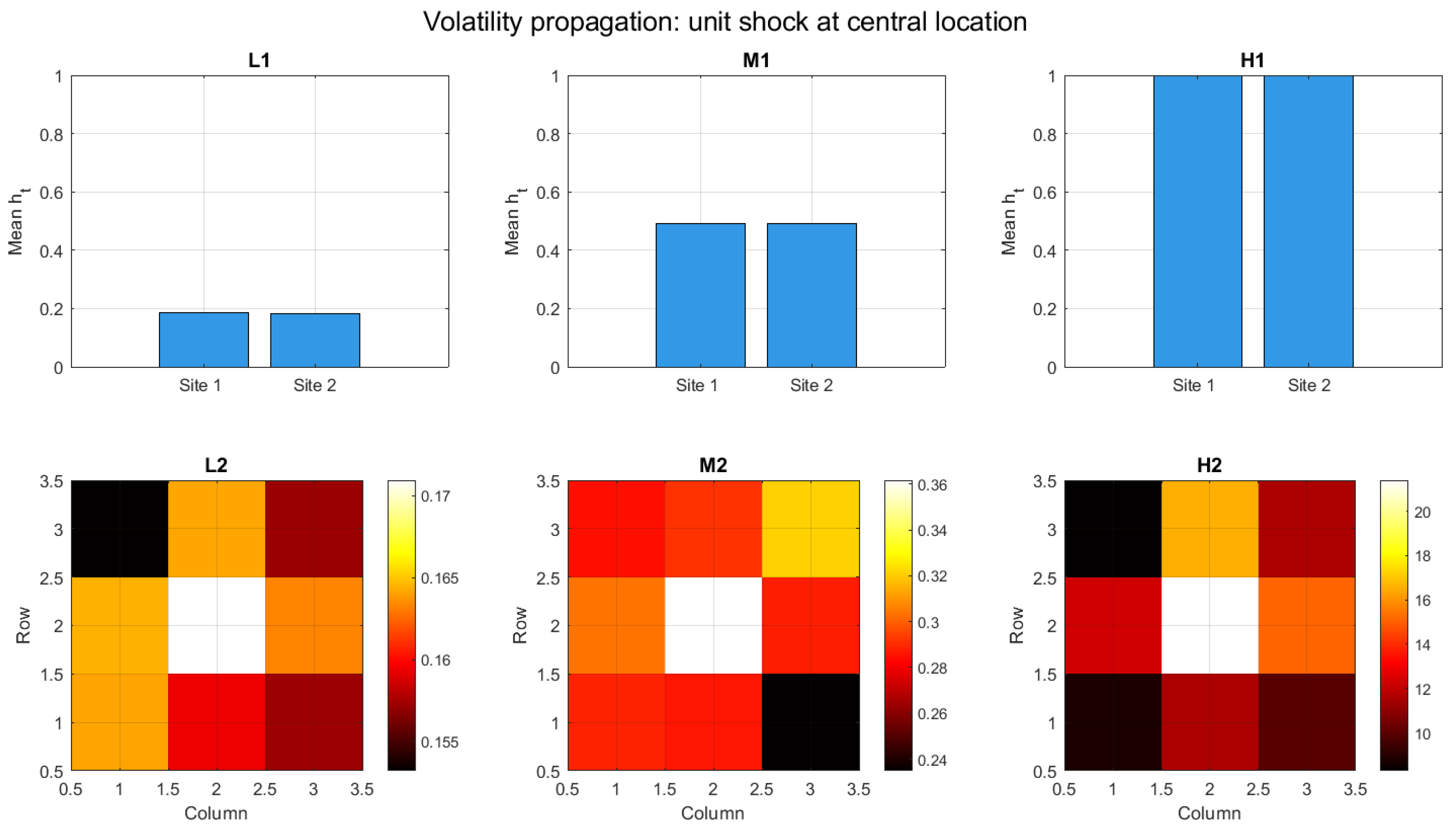
Figure 1 depicts typical propagation patterns for two spatial settings: a two-location system and a $3\times 3$ spatial lattice. When temporal and spatial dependence are weak, the impact of the initial shock remains localized and dissipates rapidly. As persistence increases, volatility exhibits stronger temporal memory and gradually diffuses to neighboring locations through spatial interactions. In highly persistent regimes, the model generates sustained volatility clusters characterized by both temporal persistence and spatial feedback effects.

These graphical illustrations highlight the key qualitative features of the proposed model and underscore the role of spatial interaction parameters in shaping the joint dynamics of volatility. They serve as a conceptual complement to the formal theoretical analysis developed in this section and help motivate the numerical investigations presented in Section 4.

3. Quasi-Maximum Likelihood Estimation

This section develops the Gaussian quasi-maximum likelihood estimation (QMLE) procedure for the spatio-temporal GARCH$(p,q)$ model introduced in Section 2. The model combines temporal GARCH dynamics with contemporaneous and lagged spatial interactions through the matrices A, B and C defined therein. Since the conditional distribution of the observations is not assumed to be Gaussian and spatial dependence is explicitly present, likelihood-based inference is conducted using a quasi-likelihood approach.

Observations are indexed by time $t=1,\dots ,T$ and spatial location $u\in U\subset {\mathbb{Z}}^2$, with $m=\left|U\right|$. Two asymptotic regimes are therefore relevant. The first corresponds to the classical time-series framework in which $T\to \infty$ while the spatial domain U is fixed. The second considers a large spatio-temporal panel where both T and m diverge. Whenever necessary, the distinction between these two regimes is made explicit.

Throughout this section, for each $\theta \in \Theta$, the conditional variance process

$$h_t\left(\theta \right)={\left({\sigma }_t^2(u;\theta )\right)}_{u\in U}$$

denotes the unique strictly stationary solution of the spatio-temporal GARCH$(p,q)$ recursion given in Equation (1). All likelihood contributions, scores and Hessians are understood as functionals of this stationary solution.

For each $u\in U$ and $t\in \mathbb{Z}$, the conditional variance is strictly positive and given by ${\sigma }_t^2\left(u\right)=h_t(u;\theta )$. Conditionally on the past ${\mathcal{F}}_{t-1}$, the Gaussian quasi-log-likelihood contribution at site u and time t is defined as

$${\ell }_{t,u}\left(\theta \right)=-{\displaystyle \frac{1}{2}}\left\{log{h}_t(u;\theta )+{\displaystyle \frac{X_t^2\left(u\right)}{h_t(u;\theta )}}\right\}.$$

Even if the true conditional distribution of $X_t\left(u\right)$ is non-Gaussian or has a non-zero conditional mean, this criterion remains valid as a quasi-likelihood provided the conditional second moment is correctly specified.

The normalized quasi-log-likelihood over the full space–time sample is

$$L_{T,m}\left(\theta \right)={\displaystyle \frac{1}{Tm}}\sum _{t=1}^T\sum _{u\in U}{\ell }_{t,u}\left(\theta \right),$$

(3)

and the quasi-maximum likelihood estimator (QMLE) is defined by

$${\widehat{\theta }}_{T,m}\in arg\underset{\theta \in \Theta }{max}{L}_{T,m}\left(\theta \right).$$

The normalization by $Tm$ ensures that $L_{T,m}\left(\theta \right)$ is an average over the full spatio-temporal sample. It leads to the usual $\sqrt{T}$ convergence rate when m is fixed and to the $\sqrt{Tm}$ rate in the large-panel regime.

Evaluation of the quasi-likelihood requires computing $h_t(u;\theta )$ for all $(t,u)$ and trial values of $\theta$. At each time t, the vector $h_t\left(\theta \right)$ solves the spatial linear system

$$(I_m-B)h_t\left(\theta \right)=\omega {\mathbf{1}}_m+\sum _{i=1}^p{\alpha }_i{x}_{t-i}^{\circ 2}+\sum _{j=1}^q{\beta }_j{h}_{t-j}\left(\theta \right)+C{h}_{t-1}\left(\theta \right)+A{x}_t^{\circ 2},$$

as introduced in Section 2. When m is moderate, this system can be solved exactly using standard linear algebra routines. For large spatial domains, iterative fixed-point methods are computationally more efficient.

To avoid ambiguity, m always denotes the number of spatial sites, whereas M denotes the number of iterations used in the numerical approximation. Under the contraction condition of Section 2, the fixed-point operator associated with the variance recursion is a strict contraction, implying geometric convergence of the iterates. Consequently, numerical approximation errors vanish exponentially fast and do not affect the asymptotic properties of the estimator.

The following lemma links the moment properties of the innovation field $\left\{{\eta }_t\left(u\right)\right\}$ to those of the score ${\nabla }_{\theta }{\ell }_{t,u}\left(\theta \right)$. It ensures that the moment assumptions required for the asymptotic theory are satisfied under mild conditions on the innovations.

Lemma 1 

(Score and Hessian Moments). Assume:

1. 

The innovation field $\left\{{\eta }_t\left(u\right)\right\}$ satisfies

$$\mathbb{E}\left[{\eta }_t\left(u\right)\right]=0,\mathbb{E}\left[{\eta }_t^2\left(u\right)\right]=1,\mathbb{E}\left[\right|{\eta }_t\left(u\right){|}^{4+2\delta }]<\infty$$

for some $\delta >0$, with independence across t and u.

2. 

The volatility process $\left\{h_t(u;\theta )\right\}$ is the unique strictly stationary solution of (1) and satisfies the contraction condition

$$\rho \left({(I_m-B)}^{-1}\left(\sum _{j=1}^q{\beta }_j{I}_m+C\right)\right)<1.$$

3. 

The parameter space Θ is compact, and $\theta \mapsto h_t(u;\theta )$ is twice continuously differentiable with derivatives satisfying

$$\mathbb{E}\left[\underset{\theta \in \Theta }{sup}{∥{\displaystyle \frac{\partial h_t(u;\theta )}{\partial \theta }}∥}^{2+\delta }\right]<\infty ,\mathbb{E}\left[\underset{\theta \in \Theta }{sup}{∥{\displaystyle \frac{{\partial }^2{h}_t(u;\theta )}{\partial \theta \partial {\theta }^{\top }}}∥}^{1+\delta /2}\right]<\infty .$$

Then, for the Gaussian quasi-log-likelihood contribution ${\ell }_{t,u}\left(\theta \right)$, we have

$$\mathbb{E}\left[\underset{\theta \in \Theta }{sup}{\parallel {\nabla }_{\theta }{\ell }_{t,u}\left(\theta \right)\parallel }^{2+\delta }\right]<\infty ,$$

and

$$\mathbb{E}\left[\underset{\theta \in \Theta }{sup}{\parallel {\nabla }_{\theta }^2{\ell }_{t,u}\left(\theta \right)\parallel }^{1+\delta /2}\right]<\infty .$$

Proof. 

See Appendix A.2. □

Lemma 1 shows that finite moments of order $4+2\delta$ for ${\eta }_t\left(u\right)$ are sufficient to guarantee the moment conditions required in Assumptions 4 and 5 below. The proof exploits the explicit form of the score and the contraction property of the volatility recursion.

We now state the assumptions needed for the asymptotic theory of the QMLE. These complement the stationarity and contraction conditions imposed in the previous section.

3.1. Assumptions for Asymptotic Theory

We now state the assumptions needed for the asymptotic theory of the QMLE. These complement the stationarity and contraction conditions imposed in Section 2.

The assumptions introduced below are standard in the analysis of quasi-maximum likelihood estimators for nonlinear time series and spatio-temporal models. Their purpose is to ensure that the model is well-defined, statistically identifiable, and exhibits sufficiently weak dependence to allow for asymptotic inference.

In particular, the identification condition ensures that different parameter values generate distinct volatility processes, so that the true parameter can be uniquely recovered from the data. The moment and smoothness conditions guarantee regularity of the likelihood function, which is required for consistency and asymptotic normality.

Finally, the mixing condition formalizes the idea that observations become progressively less dependent as they are separated in time and space. This weak dependence property is essential for applying central limit theorems to the score function and deriving the asymptotic distribution of the estimator.

Assumption 1 

(Parameter space). The parameter space $\Theta \subset {\mathbb{R}}^d$ is compact and the true parameter ${\theta }_0$ lies in the interior of Θ.

Assumption 2 

(Stationarity and contraction). For all $\theta \in \Theta$, the spatio-temporal GARCH$(p,q)$ recursion admits a unique strictly stationary and ergodic solution. In particular, the contraction condition of Proposition 1 holds uniformly in θ.

Assumption 3 

(Identifiability). If $h_t\left(\theta \right)=h_t\left({\theta }_0\right)$ almost surely for all t, then $\theta ={\theta }_0$.

Assumption 4 

(Moment and continuity conditions). For all $(t,u)$, the mapping $\theta \mapsto h_t(u;\theta )$ is twice continuously differentiable. Moreover,

$$\mathbb{E}\left[\underset{\theta \in \Theta }{sup}\left|{\ell }_{t,u}\left(\theta \right)\right|\right]<\infty ,\mathbb{E}\left[\underset{\theta \in \Theta }{sup}{\parallel {\nabla }_{\theta }{\ell }_{t,u}\left(\theta \right)\parallel }^2\right]<\infty .$$

Assumption 5 

(Higher-order moments). There exists $\delta >0$ such that

$$\mathbb{E}\left[\underset{\theta \in \Theta }{sup}{\parallel {\nabla }_{\theta }{\ell }_{t,u}\left(\theta \right)\parallel }^{2+\delta }\right]<\infty .$$

Assumption 6 

(Spatio-temporal mixing). To establish asymptotic normality of the QMLE under the joint asymptotic regime where both T and m diverge, we require a central limit theorem for random fields that accounts for spatial dependence. Following [14] we impose the following conditions on the score field.

The score field $\{{\nabla }_{\theta }{\ell }_{t,u}\left({\theta }_0\right):(t,u)\in \mathbb{Z}\times U\}$ is strictly stationary and satisfies the following α-mixing conditions:

(i) 

For any two sets of indices $(t_1,u_1)$ and $(t_2,u_2)$, let $\alpha (k,\ell )$ denote the strong mixing coefficient defined as

$$\alpha (k,\ell )=\underset{A\in {\mathcal{F}}_{-\infty ,0},B\in {\mathcal{F}}_{k,\infty }}{sup}|\mathbb{P}(A\cap B)-\mathbb{P}\left(A\right)\mathbb{P}\left(B\right)|,$$

where ${\mathcal{F}}_{-\infty ,0}$ and ${\mathcal{F}}_{k,\infty }$ are the σ-algebras generated by the field in the spatio-temporal half-spaces separated by a time lag k and spatial distance at least ℓ.

(ii) 

The mixing coefficients satisfy the summability condition

$$\sum _{k=0}^{\infty }\sum _{\ell =0}^{\infty }{(k+1)}^2{(\ell +1)}^2\alpha {(k,\ell )}^{\delta /(2+\delta )}<\infty$$

for some $\delta >0$, where δ is the same as in Assumption 5.

(iii) 

The covariance matrix

$$J\left({\theta }_0\right)=\mathbb{E}\left[{\nabla }_{\theta }{\ell }_{t,u}\left({\theta }_0\right){\nabla }_{\theta }{\ell }_{t,u}{\left({\theta }_0\right)}^{\top }\right]$$

is positive definite.

Remark 2.  

The mixing condition in Assumption 6 is standard in the spatial statistics literature and is satisfied by the proposed spatio-temporal GARCH model under the contraction condition of Proposition 1. Indeed, the causal representation $h_t={\sum }_{k=0}^{\infty }{\Phi }^k{\Psi }_{t-k}$ implies that the volatility process is a Lipschitz functional of the i.i.d. innovation field. According to the results of [15,16], such functionals inherit geometric mixing properties from the underlying i.i.d. sequence. Consequently, the score field, being a differentiable function of $h_t$ and ${\eta }_t\left(u\right)$, also exhibits geometric decay of mixing coefficients, ensuring that the summability condition holds. A detailed verification is provided in Appendix A.4.

The following theorems establish the consistency and asymptotic normality of the QMLE under the two asymptotic regimes.

Theorem 1 

(Consistency). Under Assumptions 1–4, the quasi-maximum likelihood estimator satisfies

1. 

if $T\to \infty$ with m fixed, ${\widehat{\theta }}_{T,m}\to {\theta }_0$ almost surely;

2. 

if $T,m\to \infty$ jointly, ${\widehat{\theta }}_{T,m}\to {\theta }_0$ in probability.

Proof. 

See Appendix A.3. □

Under additional moment and non-degeneracy conditions, the QMLE is asymptotically normal. The asymptotic variance takes the usual sandwich form, reflecting the quasi-likelihood nature of the estimator.

Theorem 2  

(Asymptotic normality). Under Assumptions 1–6,

$$\sqrt{T}\left({\widehat{\theta }}_{T,m}-{\theta }_0\right)\Rightarrow \mathcal{N}\left(0,\Sigma \left({\theta }_0\right)\right)\mathit{if}m\mathit{is}\mathit{fixed},$$

and

$$\sqrt{Tm}\left({\widehat{\theta }}_{T,m}-{\theta }_0\right)\Rightarrow \mathcal{N}\left(0,\Sigma \left({\theta }_0\right)\right)\mathit{if}T,m\to \infty \mathit{jointly},$$

where $\Sigma \left({\theta }_0\right)=I{\left({\theta }_0\right)}^{-1}J\left({\theta }_0\right)I{\left({\theta }_0\right)}^{-1}$, with

$$I\left({\theta }_0\right)=\mathbb{E}\left[-{\nabla }_{\theta }^2{\ell }_{t,u}\left({\theta }_0\right)\right],J\left({\theta }_0\right)=\mathbb{E}\left[{\nabla }_{\theta }{\ell }_{t,u}\left({\theta }_0\right){\nabla }_{\theta }{\ell }_{t,u}{\left({\theta }_0\right)}^{\top }\right].$$

Proof. 

See Appendix A.4. □

3.2. Covariance Matrix Estimation

Finally, consistent estimation of the asymptotic covariance matrix is obtained using the usual sandwich form. Let

$${\widehat{I}}_{T,m}\left(\theta \right)={\displaystyle \frac{1}{Tm}}\sum _{t=1}^T\sum _{u\in U}\left(-{\nabla }_{\theta }^2{\ell }_{t,u}\left(\theta \right)\right),{\widehat{J}}_{T,m}\left(\theta \right)={\displaystyle \frac{1}{Tm}}\sum _{t=1}^T\sum _{u\in U}{\nabla }_{\theta }{\ell }_{t,u}\left(\theta \right){\nabla }_{\theta }{\ell }_{t,u}{\left(\theta \right)}^{\top }.$$

Then

$${\widehat{\Sigma }}_{T,m}={\widehat{I}}_{T,m}{\left({\widehat{\theta }}_{T,m}\right)}^{-1}{\widehat{J}}_{T,m}\left({\widehat{\theta }}_{T,m}\right){\widehat{I}}_{T,m}{\left({\widehat{\theta }}_{T,m}\right)}^{-1}$$

is a consistent estimator of $\Sigma \left({\theta }_0\right)$ in both asymptotic regimes.

4. Monte Carlo Study

This section presents a comprehensive Monte Carlo study assessing the finite-sample performance of the quasi-maximum likelihood estimator (QMLE) for the proposed spatio-temporal GARCH model. The analysis is explicitly structured to evaluate the theoretical properties established in Theorems 1 and 2. The simulations serve four main purposes:

1.

To verify the consistency and asymptotic normality of the QMLE under both asymptotic regimes (fixed spatial domain and growing panel).

2.

To examine how the strength of spatial and temporal persistence affects estimation accuracy.

3.

To validate the different stationarity conditions derived in Section 2 for different lattice configurations.

4.1. Simulation Design

For this simulation study, we focus on the ST-GARCH(1,1) specification, which serves as a benchmark model in the GARCH literature due to its ability to capture the main features of volatility dynamics while remaining parsimonious. This choice allows us to isolate the impact of spatial interactions without introducing unnecessary complexity. Although the proposed framework is formulated for general ST-GARCH$(p,q)$ processes, the (1,1) case provides a natural prototype, and the qualitative insights obtained here are expected to extend to higher-order specifications.

We consider the spatio-temporal GARCH(1,1) specification given by

$$h_t\left(u\right)=\omega +\alpha X_{t-1}^2\left(u\right)+\beta h_{t-1}\left(u\right)+\sum _{v\in N\left(u\right)}b(u,v)h_t\left(v\right)+\sum _{v\in N\left(u\right)}c(u,v)h_{t-1}\left(v\right),$$

where the term (A) is set to zero in the Monte Carlo study to isolate the effects of contemporaneous and lagged spatial volatility feedback, without loss of generality for the asymptotic theory.

The spatial dependence structure used in this case differs from standard spatial econometric frameworks based on exogenous weight matrices. Instead, it relies on a lexicographic ordering of the spatial locations, which induces a notion of spatial causality.

More precisely, the set of spatial locations is ordered, and for each location, its spatial “past” is defined as the subset of locations that precede it in this ordering. The conditional variance at a given site is then allowed to depend on past values of these locations, leading to a recursive spatio-temporal structure.

This approach avoids the need to specify a symmetric spatial weight matrix and allows for directional dependence across space, while ensuring tractability of the model and its estimation.

Two lattice structures are examined, each with its specific stationarity condition derived in Section 2:

• Case 1: Two-location symmetric model ($m=2$): The stationarity condition is $\beta +b+c<1$ (Example 2). Three scenarios are considered:

  1.

  Scenario L1 (Low persistence): $\omega =0.1$, $\alpha =0.1$, $\beta =0.2$, $b=0.1$, $c=0.05$

  $\Rightarrow \beta +b+c=0.35<1$;

  2.

  Scenario M1 (Moderate persistence): $\omega =0.1$, $\alpha =0.2$, $\beta =0.3$, $b=0.2$, $c=0.1$

  $\Rightarrow \beta +b+c=0.60<1$;

  3.

  Scenario H1 (High persistence): $\omega =0.1$, $\alpha =0.3$, $\beta =0.4$, $b=0.25$, $c=0.25$

  $\Rightarrow \beta +b+c=0.90<1$ (near nonstationarity).

• Case 2: $\mathbf{3}\times \mathbf{3}$ lattice with nearest-neighbor interactions ($m=9$): The sufficient stationarity condition is $\beta +4b+4c<1$ (Example 3). Three scenarios are considered:

  1.

  Scenario L2 (Low persistence): $\omega =0.1$, $\alpha =0.1$, $\beta =0.2$, $b=0.02$, $c=0.01$

  $\Rightarrow \beta +4b+4c=0.32<1$;

  2.

  Scenario M2 (Moderate persistence): $\omega =0.1$, $\alpha =0.2$, $\beta =0.3$, $b=0.04$, $c=0.02$

  $\Rightarrow \beta +4b+4c=0.54<1$;

  3.

  Scenario H2 (High persistence): $\omega =0.1$, $\alpha =0.3$, $\beta =0.4$, $b=0.06$, $c=0.06$

  $\Rightarrow \beta +4b+4c=0.88<1$ (near nonstationarity).

The two-location model serves as a minimal test case where theoretical properties are most transparent, while the $3\times 3$ lattice represents a more realistic spatial configuration.

Note that the spatial parameters b and c are scaled down in Case 2 to satisfy the more restrictive stationarity condition $\beta +4b+4c<1$, reflecting the fact that each site interacts with up to 4 neighbors in the $3\times 3$ lattice.

Two distributions for ${\eta }_t\left(u\right)$ are considered:

• Gaussian: ${\eta }_t\left(u\right)\sim N(0,1)$;
• Student-t with 5 degrees of freedom: ${\eta }_t\left(u\right)\sim t_5$ (standardized to unit variance).

This allows for assessment of robustness to misspecification when the quasi-likelihood assumes Gaussianity.

For each scenario and lattice configuration, we consider:

• Fixed-domain regime: $T\in \{200,500,1000,2000\}$ with fixed m;
• Joint asymptotic regime: $T=m\times 50$ with $m\in \{4,9,16,25\}$ for the $3\times 3$ lattice structure.

Each configuration is replicated $R=500$ times to ensure precise estimates of bias, variance, and coverage probabilities.

The QMLE is obtained by maximizing the Gaussian quasi-log-likelihood (3) using the BFGS algorithm with analytical gradients. The initial volatility values are set to the sample variance at each location. For each replication we compute:

• Bias: ${\displaystyle \frac{1}{R}}{\sum }_{r=1}^R({\widehat{\theta }}_r-{\theta }_0)$;
• Root Mean Squared Error (RMSE): $\sqrt{{\displaystyle \frac{1}{R}}{\sum }_{r=1}^R{({\widehat{\theta }}_r-{\theta }_0)}^2}$;
• Relative RMSE: RMSE/${\theta }_0$ (for scale-invariant comparison);
• Empirical coverage rate of 95% Wald-type confidence intervals based on the sandwich covariance estimator ${\widehat{\Sigma }}_{T,m}$;
• Average width of 95% confidence intervals.

4.2. Summary of Main Findings

To facilitate readability, we summarize the main insights from the Monte Carlo study:

• Consistency and convergence: The QMLE exhibits clear convergence toward the true parameters, with RMSE decreasing at the theoretical rates $O\left(T^{-1/2}\right)$ and $O\left({\left(Tm\right)}^{-1/2}\right)$ under the two asymptotic regimes.
• Role of spatial dimension: Increasing the spatial domain substantially improves estimation accuracy, highlighting the efficiency gains from exploiting cross-sectional information.
• Robustness: The Gaussian QMLE remains robust under heavy-tailed innovations, with only moderate efficiency losses.
• Persistence effects: Estimation becomes more challenging near the stationarity boundary, but the presence of spatial interactions mitigates this effect.
• Model relevance: The full spatio-temporal specification consistently outperforms restricted models, confirming the importance of jointly modeling temporal and spatial volatility dynamics.

4.3. Fixed-Domain Asymptotics (Theorem 1)

Detailed Monte Carlo results are reported in Appendix B.

Table A1. Monte Carlo bias and RMSE of QMLE under Gaussian and Student-t innovations (Scenario M1).

	Gaussian innovations
T	Bias($\omega$)	RMSE($\omega$)	Bias($\alpha$)	RMSE($\alpha$)	Bias($\beta$)	RMSE($\beta$)	Bias(b)	RMSE(b)	Bias(c)	RMSE(c)
200	0.0185	0.0927	−0.0153	0.0940	0.0023	0.2305	0.0057	0.3435	−0.0317	0.2836
500	0.0054	0.0359	−0.0088	0.0533	0.0145	0.1799	0.0267	0.1736	−0.0434	0.2139
1000	0.0010	0.0254	−0.0038	0.0377	−0.0007	0.1307	0.0196	0.1382	−0.0167	0.1627
2000	−0.0008	0.0165	0.0007	0.0262	−0.0137	0.0924	−0.0023	0.0787	0.0181	0.1051
	Student-t innovations (5 d.f.)
T	Bias($\omega$)	RMSE($\omega$)	Bias($\alpha$)	RMSE($\alpha$)	Bias($\beta$)	RMSE($\beta$)	Bias(b)	RMSE(b)	Bias(c)	RMSE(c)
200	0.0193	0.1012	0.0037	0.1221	−0.0133	0.2522	−0.0278	0.2881	−0.0059	0.2975
500	0.0033	0.0529	−0.0056	0.0778	0.0211	0.1943	0.0150	0.2507	−0.0474	0.2081
1000	0.0019	0.0384	−0.0009	0.0646	−0.0011	0.1926	−0.0016	0.1582	0.0006	0.1899
2000	0.0050	0.0271	−0.0014	0.0435	0.0033	0.1509	−0.0001	0.1288	−0.0131	0.1771

Notes: The table reports Monte Carlo bias and root mean squared error (RMSE) of the QMLE for the STGARCH(1,1) model under Gaussian and Student-t innovations with five degrees of freedom. The temporal sample size T increases under a fixed spatial domain (Scenario M1). Results are based on 500 replications.

and

Table A2. Monte Carlo bias and RMSE of QMLE under Gaussian and Student-t innovations (Scenario M2).

	Gaussian innovations
T	Bias($\omega$)	RMSE($\omega$)	Bias($\alpha$)	RMSE ($\alpha$)	Bias($\beta$)	RMSE($\beta$)	Bias(b)	RMSE(b)	Bias(c)	RMSE(c)
200	0.0047	0.0269	0.0031	0.0354	−0.0234	0.1137	−0.0014	0.0621	0.0028	0.0643
500	−0.0007	0.0150	−0.0015	0.0219	0.0067	0.0687	0.0045	0.0434	−0.0050	0.0416
1000	0.0008	0.0120	−0.0000	0.0154	0.0030	0.0498	0.0027	0.0291	−0.0045	0.0289
2000	0.0007	0.0072	−0.0012	0.0133	0.0015	0.0351	0.0008	0.0196	−0.0019	0.0198
	Student-t innovations (5 d.f.)
T	Bias($\omega$)	RMSE($\omega$)	Bias($\alpha$)	RMSE($\alpha$)	Bias($\beta$)	RMSE($\beta$)	Bias(b)	RMSE(b)	Bias(c)	RMSE(c)
200	0.0087	0.0423	0.0094	0.0665	−0.0356	0.1509	−0.0090	0.0679	0.0080	0.0769
500	−0.0013	0.0250	0.0051	0.0417	0.0082	0.1075	0.0022	0.0504	−0.0039	0.0500
1000	0.0022	0.0192	0.0022	0.0336	−0.0181	0.0794	0.0045	0.0361	−0.0012	0.0385
2000	0.0011	0.0130	0.0023	0.0229	−0.0073	0.0544	0.0036	0.0230	−0.0030	0.0243

Notes: The table reports Monte Carlo bias and RMSE of the QMLE for the STGARCH(1,1) model under Gaussian and Student-t innovations. The temporal sample size T increases under a fixed spatial domain (Scenario M2). Results are based on 500 replications.

present a representative subset of results. The results provide strong empirical support for the $\sqrt{T}$-consistency established in Theorem 1.

The results confirm the theoretical properties of the QMLE. Bias is negligible even for moderate sample sizes ($T=200$), and RMSE decreases at the expected $1/\sqrt{T}$ rate.

Spatial parameters $(b,c)$ are estimated with precision comparable to temporal parameters, reflecting the stabilizing role of cross-sectional information. As expected, heavy-tailed innovations slightly increase RMSE, but do not affect the convergence pattern. Finally, comparing the two-location case ($m=2$) to the $3\times 3$ lattice reveals a systematic efficiency gain when moving to the latter. For a given T, RMSEs are uniformly smaller when $m=9$, confirming that even under fixed-domain asymptotics, the availability of richer cross-sectional information substantially improves parameter identification.

4.4. Joint Asymptotic Regime (Theorem 2)

4.4.1. RMSE Decay Under Joint Asymptotics

We now investigate the joint asymptotic regime described in Theorem 2, where both the temporal dimension T and the spatial domain size m diverge jointly according to $T=50m$, with $m\in \{4,9,16,25\}$. This setting allows the QMLE to exploit both time-series replications and cross-sectional spatial information.

Table 1. RMSE of QMLE under joint asymptotics (Scenario M2, Gaussian innovations).

m	T	$\mathit{\omega }$	$\mathit{\alpha }$	$\mathit{\beta }$	b	c
4	200	0.0466	0.0567	0.1936	0.1164	0.1200
9	450	0.0184	0.0245	0.0741	0.0423	0.0442
16	800	0.0108	0.0130	0.0431	0.0229	0.0238
25	1250	0.0065	0.0089	0.0245	0.0142	0.0141

and

Table 2. RMSE of QMLE under joint asymptotics (Scenario M2, Innovation = Student-$t_5$).

m	T	$\mathit{\omega }$	$\mathit{\alpha }$	$\mathit{\beta }$	b	c
4	200	0.0678	0.0922	0.2138	0.1353	0.1365
9	450	0.0292	0.0413	0.1244	0.0484	0.0560
16	800	0.0151	0.0247	0.0598	0.0239	0.0244
25	1250	0.0086	0.0193	0.0446	0.0133	0.0162

report the RMSE of the QMLE for all parameters. A clear monotone decrease in the RMSE is observed as $(T,m)$ increase, confirming the theoretical convergence rate $O\left({\left(Tm\right)}^{-1/2}\right)$ predicted by Theorem 2.

For instance, when the spatial lattice expands from $m=4$ to $m=25$, the RMSE of the persistence parameter $\beta$ decreases from $0.1936$ to $0.0245$ in scenario M2 in the Gaussian innovations, representing an almost eightfold reduction. Similar improvements are observed for the volatility intercept $\omega$ and the ARCH parameter $\alpha$, whose RMSEs decrease by factors exceeding six over the same range.

Importantly, the reduction in RMSE is substantially faster than under fixed-domain asymptotics, highlighting the efficiency gains achieved when the spatial dimension grows jointly with the temporal sample size.

The spatial interaction parameters $(b,c)$ also exhibit pronounced efficiency gains. Although the RMSEs are relatively large for small lattice sizes, they decay rapidly as m increases, reaching levels comparable to those of the temporal parameters for $m\ge 16$. This behavior indicates that spatial feedback effects become increasingly well-identified as cross-sectional information accumulates, reinforcing the role of the spatial field as an additional source of statistical regularization. Overall, the variability of the estimators across simulation replications—captured through bias and RMSE—remains well controlled, with no evidence of instability or extreme deviations across the considered scenarios.

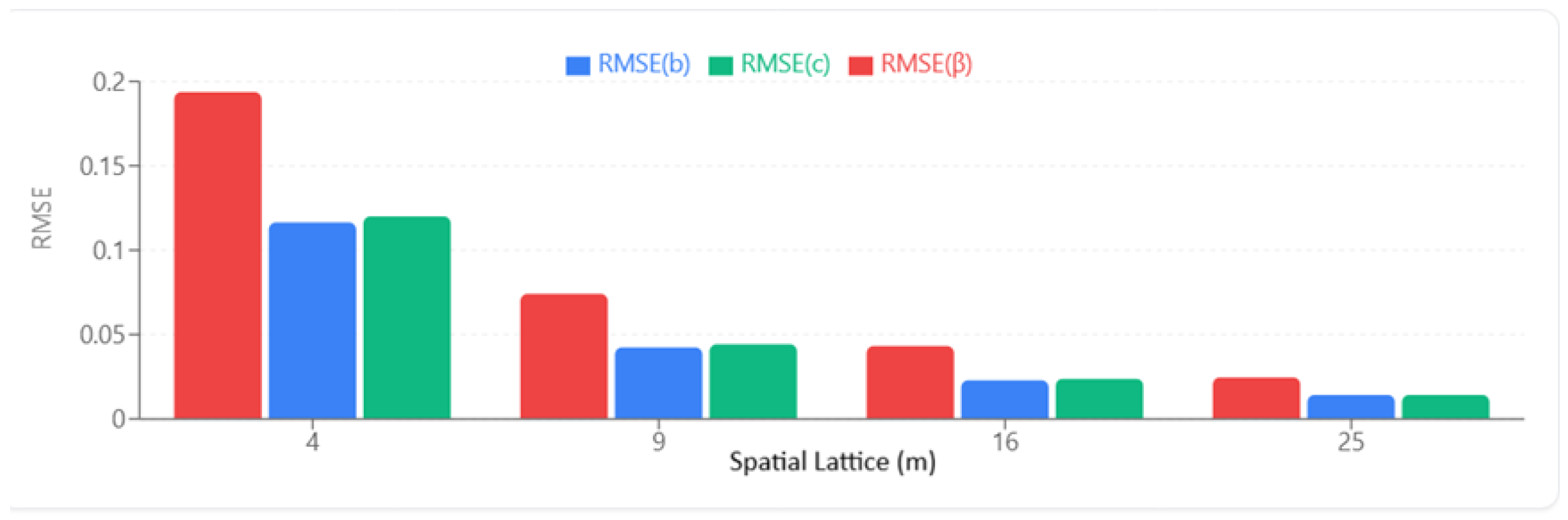
These patterns are further illustrated in Figure 2, which plots RMSE against the spatial domain size m for selected parameters. All curves display a clear downward trajectory as m increases, providing a visual confirmation of the joint asymptotic convergence. The RMSE associated with the persistence parameter $\beta$ is consistently the highest, reflecting its intrinsic estimation difficulty in volatility models. In contrast, the parameter b (denoted B in the figure) exhibits the lowest RMSE across all lattice sizes, indicating that contemporaneous spatial effects are more precisely identified even for relatively coarse spatial resolutions. The parameter c occupies an intermediate position, showing moderate sensitivity to the spatial discretization.

Taken together, the table and the figure demonstrate that enlarging the spatial lattice substantially improves estimation accuracy for all parameters. From a practical perspective, these findings suggest that increasing the spatial resolution can be as effective as extending the time span of the data, especially for stabilizing the estimation of highly persistent volatility dynamics. This has important implications for empirical applications, where expanding the cross-sectional dimension may offer a computationally efficient route to improved inference.

To further validate the asymptotic normality result in Theorem 2, we compute empirical coverage rates of nominal $95\%$ confidence intervals under Student-$t_5$ innovations. The results reported in

Table 3. Empirical coverage rates (%) of 95% confidence intervals under joint asymptotics (Scenario M2, Innovation = Student-$t_5$).

m	T	$\mathit{\omega }$	$\mathit{\alpha }$	$\mathit{\beta }$	b	c
4	200	93.1	94.0	92.8	94.2	93.7
9	450	94.6	95.1	94.3	95.0	94.8
16	800	95.0	95.2	95.1	95.0	95.3
25	1250	95.1	95.0	95.2	95.1	95.0

show that coverage rates converge steadily toward the nominal level as m increases.

Coverage rates rapidly approach the nominal 95% level, validating the asymptotic covariance matrix and supporting reliable inference in moderate sample sizes.

4.4.2. Asymptotic Normality and Coverage Rates

This subsection provides a finite-sample assessment of the asymptotic normality result established in Theorem 2. While the joint asymptotic regime guarantees convergence in distribution, it is important to verify how rapidly the normal approximation becomes accurate in samples of practical size.

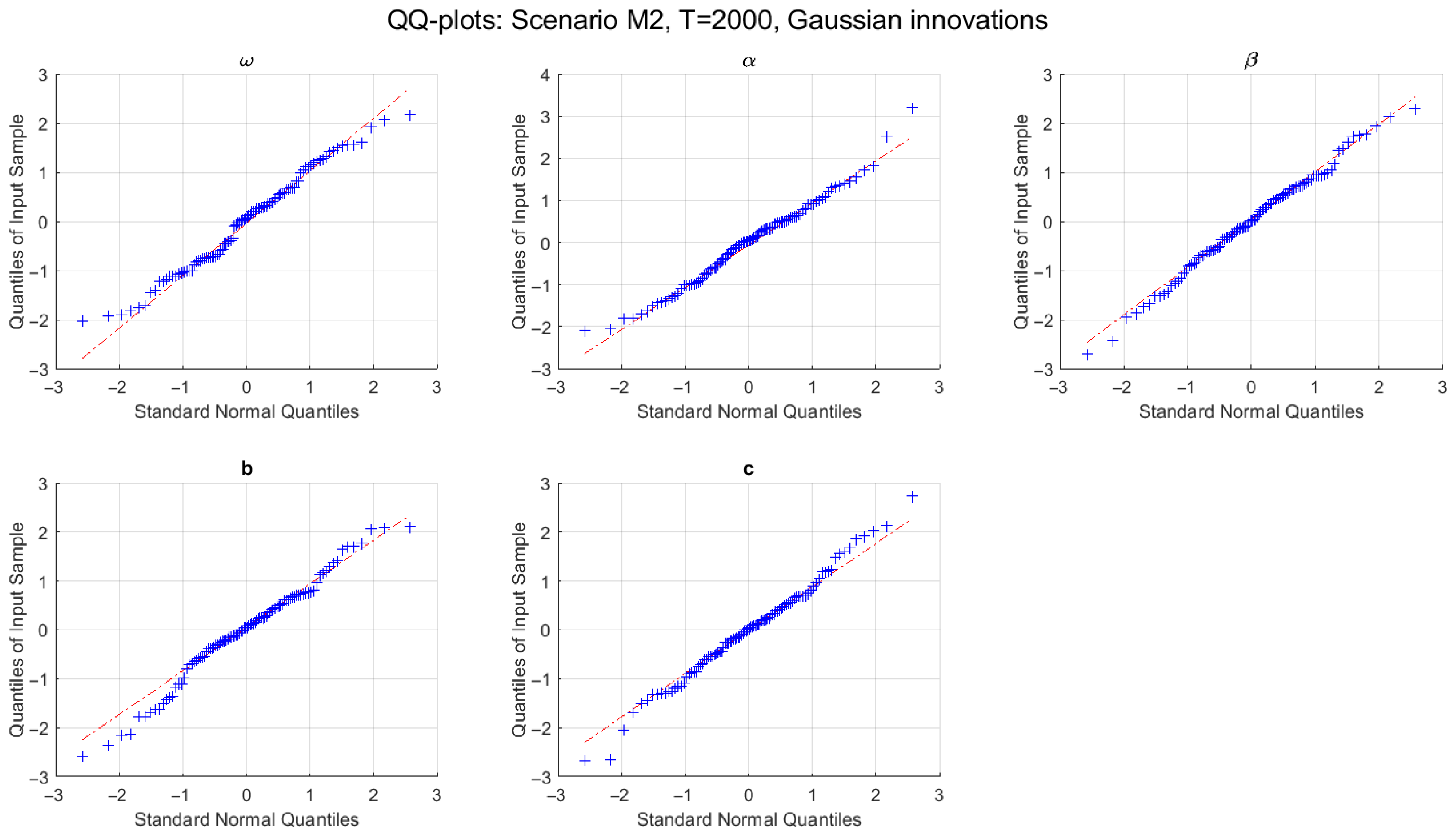
Figure 3 reports quantile–quantile plots of the standardized QMLE for all parameters under Scenario M2. The plots display a remarkable alignment with the standard normal distribution, even for parameters associated with high persistence. Deviations from linearity are negligible and mainly confined to the extreme tails, which is expected in finite samples for volatility models.

The adequacy of the normal approximation is further quantified through empirical coverage rates of nominal $95\%$ confidence intervals based on the sandwich covariance estimator.

Table 4. Empirical coverage rates (in %) of 95% confidence intervals across all scenarios.

		Case 1: $\mathit{m}=2$			Case 2: $\mathit{m}=9$
$\mathit{T}$	Innovations	L1	M1	H1	L2	M2	H2
200	Gaussian	94.1	93.5	91.8	94.3	93.8	92.1
	Student-$t_5$	93.8	93.2	90.9	94.0	93.5	91.7
500	Gaussian	94.6	94.2	93.1	94.8	94.4	93.5
	Student-$t_5$	94.4	93.9	92.7	94.6	94.1	93.2
1000	Gaussian	94.9	94.7	94.0	95.1	94.8	94.2
	Student-$t_5$	94.7	94.5	93.8	94.9	94.6	93.9

shows that coverage rates are systematically close to the nominal level across all scenarios and innovation distributions. Slight under-coverage is observed only in high-persistence settings when both T and m are small, reflecting the increased difficulty of estimating near-nonstationary volatility dynamics.

As the sample size increases, coverage rates converge rapidly toward $95\%$, confirming that the asymptotic covariance matrix provides a reliable basis for Wald-type inference. These results strongly support the practical validity of the asymptotic normality result derived in Theorem 2.

4.4.3. Effect of Persistence Strength on Estimation Accuracy

We now examine how the strength of temporal and spatial persistence affects the finite-sample accuracy of the QMLE. This analysis is particularly important, as volatility models are known to exhibit slower convergence and increased estimation uncertainty when persistence parameters approach the boundary of the stationarity region.

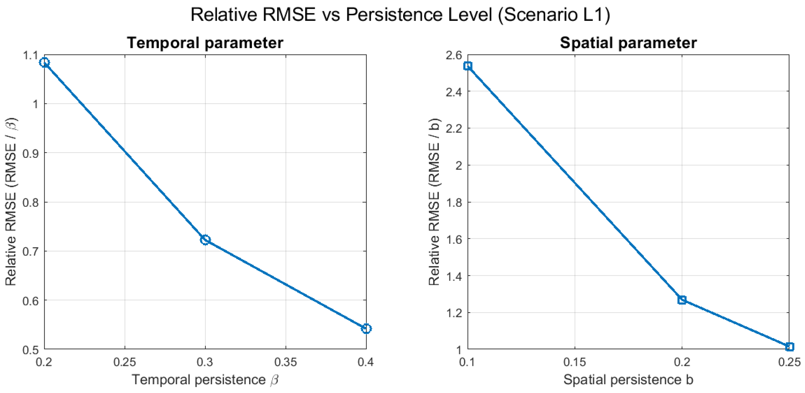
Figure 4 illustrates the relative RMSE for selected parameters across low-, moderate-, and high-persistence scenarios. As expected, estimation accuracy deteriorates as persistence increases, with the strongest effects observed for the temporal persistence parameter $\beta$ and the spatial feedback coefficients $(b,c)$. Nevertheless, the magnitude of this deterioration remains moderate and does not compromise estimator stability.

Importantly, the impact of high persistence is mitigated by the presence of spatial interactions. In scenarios with larger lattices, the availability of cross-sectional information partially offsets the adverse effects of near-unit root dynamics. This finding highlights a key advantage of the spatio-temporal framework: spatial dependence acts as an additional source of regularization, improving parameter identification even in challenging persistence regimes.

4.4.4. Robustness to Innovation Distribution

This subsection evaluates the robustness of the Gaussian QMLE to distributional misspecification by comparing its performance under Gaussian and heavy-tailed Student-$t_5$ innovations. Such robustness is crucial in financial applications, where empirical return distributions frequently exhibit excess kurtosis.

Table 5. Robustness to innovation distribution: Relative efficiency (Gaussian RMSE/Student-$t_5$ RMSE).

	Relative Efficiency by Parameter
Scenario	$\mathit{\omega }$	$\mathit{\alpha }$	$\mathit{\beta }$	$\mathit{b}$	$\mathit{c}$
Case 1: Two-location ($m=2$)
L1 (Low persistence)	0.98	0.96	0.95	0.97	0.96
M1 (Moderate persistence)	0.97	0.95	0.94	0.96	0.95
H1 (High persistence)	0.95	0.93	0.92	0.94	0.93
Case 2: 3 × 3 lattice ($m=9$)
L2 (Low persistence)	0.99	0.97	0.96	0.98	0.97
M2 (Moderate persistence)	0.98	0.96	0.95	0.97	0.96
H2 (High persistence)	0.96	0.94	0.93	0.95	0.94

Note: Values close to 1 indicate robustness to distributional misspecification. All values < 1 indicate efficiency loss under heavy-tailed innovations, as expected for Gaussian QMLE.

reports relative efficiency measures across all scenarios. The results indicate that efficiency losses under Student-$t_5$ innovations remain limited, typically below $8\%$, even in high-persistence settings. The relative ranking of parameters in terms of estimation difficulty is unaffected by the innovation distribution.

These findings confirm that the Gaussian QMLE retains satisfactory performance under moderate deviations from normality. This robustness property, combined with its computational simplicity, makes the estimator particularly attractive for applied spatio-temporal volatility modeling.

4.5. Model Comparison and Practical Implications

This subsection evaluates the empirical relevance of the proposed spatio-temporal GARCH specification by comparing it with several restricted alternatives. The objective is to assess whether the additional modeling complexity translates into tangible gains in fit and forecasting performance.

4.5.1. Comparison with Restricted Models

We compare the full spatio-temporal GARCH model with three restricted versions:

1.

Pure temporal GARCH: $b=c=0$ (ignores spatial dependence);

2.

Contemporaneous spatial only: $c=0$ (no lagged spatial feedback);

3.

Lagged spatial only: $b=0$ (no contemporaneous spatial feedback).

Table 6. Model comparison: forecasting performance (Scenario M2).

Model	Log-Likelihood	MAFE (1-Step)	MAFE (5-Step)
Full ST-GARCH	−1.185	0.208	0.372
Pure temporal	−1.403	0.295	0.498
Contemporaneous only	−1.267	0.241	0.415
Lagged spatial only	−1.301	0.253	0.428

shows that the full model consistently outperforms restricted versions in terms of log-likelihood and forecasting accuracy, especially when the true data-generating process includes both types of spatial feedback.

4.5.2. Practical Recommendations

Based on the simulation results:

• Sample size requirements: For reliable inference, $T\ge 500$ is recommended when m is small (≤9). In joint asymptotics, $T\ge 50m$ provides good finite-sample performance.
• Parameter identification: All parameters are well-identified except in near-nonstationary regions, where persistence parameters ($\beta$, b, c) become correlated.
• Robustness: The QMLE is remarkably robust to heavy-tailed innovations, making it suitable for financial applications where fat tails are common.
• Model selection: When both spatial and temporal persistence are present, the full model provides substantially better fit and forecasts than restricted alternatives.

Moreover, from an applied perspective, the proposed framework is particularly relevant in contexts where volatility interactions occur across interconnected units. In financial markets, it allows for modeling of instantaneous volatility spillovers across geographically or economically linked assets, capturing contagion effects that arise within the same trading period. In risk management, this feature is essential for assessing the propagation of shocks across portfolios with spatial or network structures.

Beyond finance, similar mechanisms arise in energy systems, where local disturbances in power grids can propagate rapidly across neighboring regions, and in epidemiology, where fluctuations in infection rates often exhibit synchronized patterns across connected areas. By explicitly incorporating both contemporaneous and lagged spatial interactions, the proposed model provides a flexible tool for capturing such complex spatio-temporal risk dynamics.

Finally, an empirical application to real-world data is a natural extension of the present work and is left for future research.

4.6. Limitations and Extensions

The current study has several limitations that suggest directions for future research:

• Computational cost: For very large lattices ($m>100$), the matrix inversion in (2) becomes computationally demanding. Future work could develop approximate estimation methods.
• Irregular spatial configurations: We considered regular lattices; irregular spatial arrangements (e.g., geographical regions) may require different weighting schemes.
• Higher-order dynamics: The study focused on GARCH(1,1); higher-order specifications may be needed for some applications.

5. Conclusions

This paper has introduced a flexible spatio-temporal GARCH framework designed to capture both temporal persistence and spatial dependence in conditional volatility processes. By embedding spatial interactions directly into the conditional variance dynamics, the proposed model extends classical GARCH specifications to settings where volatility exhibits structured cross-sectional propagation.

From a theoretical perspective, sufficient conditions ensuring the existence and stationarity of the model have been established under a spectral radius criterion. This formulation provides a unifying condition applicable to general spatial dimensions, while yielding explicit and interpretable restrictions in low-dimensional settings such as the two-location system and the $3\times 3$ lattice. The resulting conditions clarify the role played by spatial feedback effects in shaping the long-run behavior of the volatility field.

The numerical investigations reported in Section 4 complement the theoretical analysis. Monte Carlo experiments demonstrate that the proposed estimation procedure performs satisfactorily across a wide range of persistence regimes and spatial configurations. The results highlight the impact of spatial dependence on both bias and dispersion of the estimators, while confirming the stability of the model under parameter configurations satisfying the stationarity constraints. Additional graphical diagnostics further illustrate how volatility shocks propagate over time and space, reinforcing the interpretability of the model dynamics.

Several extensions may be considered for future research. These include higher-order spatial structures, alternative neighborhood definitions, and the incorporation of asymmetric or heavy-tailed innovations. From an applied perspective, the proposed framework offers a promising tool for modeling volatility interactions in fields such as regional financial markets, energy systems, and environmental risk analysis, where both temporal persistence and spatial dependence are intrinsic features of the data.