Article

Multi-Soliton Solutions for the Combined KdV–mKdV Equation in Terms of Wronskian with Multi-Wave and Periodic Cross-Kink Dynamics


1
Department of Mathematics and Statistics, College of Science, Imam Mohammad Ibn Saud Islamic University (IMSIU), Riyadh 11564, Saudi Arabia
2
Center for High Energy Physics, University of the Punjab, Quaid-e-Azam Campus, Lahore 54590, Pakistan
3
Institute of Mathematics, University of the Punjab, Quaid-e-Azam Campus, Lahore 54590, Pakistan
*
Author to whom correspondence should be addressed.
Mathematics 2026, 14(9), 1488; https://doi.org/10.3390/math14091488
Submission received: 30 January 2026 / Revised: 5 April 2026 / Accepted: 16 April 2026 / Published: 28 April 2026

Abstract

This article examines the integrability of the combined KdV-mKdV equation, which provides an effective framework for modeling coherent structures in turbulent flows. We generate the explicit Darboux solutions for the combined KdV-mKdV equation using Wronskians. These results are further generalized to the K-th order and supplemented as the logarithmic derivative of the K-th order Wronskian that provides us with the multi-soliton solutions. We generate the exact explicit solution for one-, two-, and three-solitons. Graphical depictions of the soliton formations’ interactions, dynamical characteristics, and temporal evolution are used to support these conclusions. Furthermore, we generate the multi-wave and periodic cross-kink wave solutions by employing bilinear formulism. The graphical representations of these nonlinear excitations highlight their extensive dynamical activity and structural complexity.

1. Introduction

The majority of real-world systems behave nonlinearly and change dynamically throughout time. Since time is always changing, effectively modeling such systems is extremely difficult and frequently requires the use of mathematical formulations stated as nonlinear partial differential equations (NLPDEs). Integral nonlinear partial differential equations have surfaced in a number of theoretical physics and applied mathematics domains [1,2]. NLPDEs are important mathematical tools for fully representing a variety of natural phenomena and mechanisms. Numerous engineering disciplines and applied sciences, including plasma physics, mathematical biology, biophysics, optical fibers, solid-state physics, fluid dynamics, nonlinear optics, and population dynamics, use NLPDEs [3,4,5]. NLPDEs offer a useful framework for simulating the intricate dynamics of neutrally buoyant plumes in curved absorbent media in fluid mechanics [6]. A notable class of solutions to such equations is given by solitons, which are self-reinforcing, localized wave structures that arise from a subtle balance between nonlinearity and dispersion. Solitons have been the subject of ongoing research since John Scott Russell discovered them in 1834. Their mathematical foundation was solidified in the 1960s through exact analytical solutions of fundamental equations like the Korteweg–de Vries (KdV) and nonlinear Schrödinger (NLS) equations. As a result of these advancements, the KdV-mKdV equation, which covers a wide range of nonlinear excitations and offers a solid foundation for examining integrable structures, is one example of a generalized and integrated model that has gained attention.
The KdV equation, one of the oldest and most well-known soliton models, has long served as a foundation for simulating shallow-water wave propagation and examining their geometric characteristics [7]. In addition to its importance in fluid mechanics, this equation serves as an integrable model for studying electron-plasma interactions in hollow cylindrical geometries [8]. The emergence of NLPDEs in the large context of interaction theory emphasizes the necessity of efficient integrable techniques for obtaining exact solutions that disclose crucial geometric and physical characteristics of nonlinear systems. In Bose–Einstein condensate research, different kinds of solitons, including bright, dark, vortex, and gap solitons, have been found to be important characteristics of matter-wave excitations [9,10,11,12].
Soliton solutions are an essential part of the theoretical foundation for optical communications in real-world applications, demonstrating the concrete usefulness of nonlinear phenomena. Mathematicians and physicists are increasingly interested in developing efficient methods for solving nonlinear partial differential equations (NLPDEs) [13]. The most widely employed methods include the Bäcklund transformation [14], the inverse scattering transform [15] and the Darboux transformation [16,17,18,19], each playing a distinctive role in the development of integrable systems theory. Together, these methods highlight the breadth of analytical tools available and the ongoing progress in tackling complex nonlinear problems, thereby enhancing our understanding of nonlinear wave dynamics and their applications in optical communications.
In this study, we focus on constructing multi-soliton solutions of the combined Korteweg–de Vries and modified Korteweg–de Vries (KdV-mKdV) equation [20]. The combined KdV-mKdV model provides an effective framework for analyzing water phenomena, offering valuable insights into the characterization and prediction of diverse wave behaviors [21]. Its general form is given by: [22]
m t + m x x x 6 m m x + 6 a m 2 m x = 0 .
Here, m = m | ( x , t ) is a potential function. a is a real constant parameter that controls the strength of the cubic nonlinear term. In particular, when a = 0 , Equation (1) reduces to the classical KdV equation, while for nonzero a the equation represents the combined KdV-mKdV model. The combined KdV-mKdV soliton system describes the evolution of long-wavelength waves encompassing both large and small amplitudes, providing an effective framework for modeling coherent structures in turbulent flows. Among soliton equations, the combined KdV-mKdV equation has been used to simulate thermal pulses, acoustic waves, and bound-particle wave propagation [21,23].
In this study, we use the Darboux transformation (DT) to generate multi-soliton solutions for the combined KdV-mKdV equation. The DT is widely recognized as the most powerful technique in the theory of integrable systems [24,25,26], providing exact solutions that capture both algebraic and geometric features. Its physical significance has been demonstrated through numerous applications in the literature, including solving electrodynamical problems [27], modeling quantum cavity phenomena, and identifying persistent solutions with the algebraic structure of graphene [28]. Furthermore, the DT has been instrumental in generating quasi-determinant solutions [29] and related Toda systems [30]. Notably, the generation of multi-soliton solutions for dispersionless integrable systems remains a topic of significant interest.
The DT, as systematically developed in the theory of integrable systems by [24] and further elaborated by [25], provides an algebraic framework for generating new solutions from known seed solutions while preserving the associated Lax pair structure. Compared with the inverse scattering transform, the generalized DT offers a direct and constructive algebraic procedure for generating higher-order solutions and lends itself naturally to determinant formulas and potential noncommutative extensions; however, unlike spectral methods, it does not provide global scattering data.
Although the multi-soliton solutions of the combined KdV-mKdV have been previously obtained via the inverse scattering transform and Hirota’s bilinear method (see, e.g., refs. [14,15,22,23]), those approaches primarily focus on spectral analysis or bilinear representations. In contrast, the Darboux transformation provides an algebraic and iterative mechanism for generating higher-order solutions from seed configurations. A systematic K-fold Darboux transformation expressed explicitly in Wronskian determinant form for the combined KdV-mKdV has not been presented in the existing literature. The present work fills this gap by constructing a generalized Darboux framework that yields a compact determinant expression for multi-soliton solutions and facilitates further generalizations.
This paper is organized into five sections. Following the Introduction, Section 2 utilizes the equivalent linear representation of the function m to construct multi-fold Darboux system solutions. Section 3 formulate the K-fold Darboux transformation in terms of Wronskian determinants. In Section 4, multi-soliton solutions are derived by considering the trivial case m = 0 , accompanied by graphical illustrations that highlight their dynamical features. Section 5 is devoted to the derivation of multi-wave and periodic cross-kink solutions, together with their visual representations and analysis of their physical significance. The concluding remarks are presented in Section 6.

2. Lax Representation and the Darboux Solutions

This section presents the zero-curvature condition for system (1) together with its Lax representation, derived from a scalar Lax pair. A gauge transformation is then applied to shift the field variable into the off-diagonal form. Subsequently, the one-fold, two-fold, and three-fold Darboux solutions associated with the field variables are constructed from seed solutions by applying the Darboux transformation [24] to an arbitrary function. Finally, the method is extended to obtain the N-fold Darboux solutions, expressed in determinant form [31].

2.1. Lax Pair

The combined KdV-mKdV Equation (1) emerges as the compatibility requirement of linear system: [32,33]
χ x = U χ ,
χ t = V χ ,
where U and V are:
U = ι λ ι q ι m ι λ ,
V = 4 ι λ 3 1 0 0 1 4 ι λ 2 0 q m 0 + 2 λ m q ι q x ι m x r q + q m x m q x ι q x x + 2 ι m q 2 ι m x x + 2 ι m m 2 q m x m q x .
In this case, q = a m 1 . We choose the convenient option a = 1 because the analysis focuses on the combined KdV–mKdV equation.

2.2. Gauge Transformation and Zero-Curvature Representation

Consider the matrix: G = 1 2 ι ι 1 1 , which transforms the original Lax pair ( U , V ) given in Equations (4) and (5) into a new pair according to U ˜ = G U G 1 , V ˜ = G V G 1 . The new Lax pair ( U ˜ , V ˜ ) has the following form:
U ˜ = ι m ι 2 λ 1 2 λ 1 2 ι m + ι 2 ,
V ˜ = a b c d ,
where:
a = ι m x x + 2 ι m 3 + ι m 3 ι m 2 4 ι λ 2 m + 2 ι λ 2 ,
b = 4 λ 3 + 2 ι λ m 2 2 ι λ m + ι m m x ι m x + 2 λ 2 2 λ m x + m m 2 ,
c = 4 λ 3 2 ι λ m 2 + 2 ι λ m ι m m x + ι m x + 2 λ 2 2 λ m x + m 3 + m + 2 m 2 ,
d = 4 ι λ 2 m ι m x x 2 ι m 3 + 3 ι m 2 2 ι λ 2 ι m m m x ,
with the linear system:
χ x = U ˜ χ , χ t = V ˜ χ .

2.3. Darboux Solutions

To construct the Darboux solutions for the field variable m, let m [ 1 ] denote the new solution of the combined KdV–mKdV Equation (1), and let χ [ 1 ] be the corresponding linear system’s solution. The components of the column vector χ = ( X / Y ) , when subjected to the conventional Darboux transformation, yield:
X X [ 1 ] = λ Y λ 1 ( Y 1 X 1 ) X ,
Y Y [ 1 ] = λ X λ 1 ( X 1 Y 1 ) Y .
The linear system (12), when subjected to the Darboux transformation given by (13) and (14), is transformed into the given form:
X [ 1 ] = ( ι m [ 1 ] ι 2 ) X [ 1 ] ( λ + 1 2 ) Y [ 1 ] ,
Furthermore, applying relation (12) yields:
X [ 1 ] = λ Y λ 1 ( Y 1 X 1 ) X λ 1 Y 1 X 1 X ,
by combining Equations (15) and (16) and performing simplification, the 1-fold Darboux transformation is obtained in the form:
m [ 1 ] = 1 m + λ 1 ι ( Y 1 X 1 X 1 Y 1 ) ,
This expression can equivalently be written as follows:
m [ 1 ] = 1 m ι d d x l n X 1 Y 1 .
In the above expression, the field variable m links the previous solutions of the combined KdV–mKdV Equation (1) to the new ones via a particular solution of the linear system (12).

3. Generalized Darboux Solutions in Terms of Wronskians

In this section, the Darboux transformation is generalized using the Wronskian framework. Specifically, the iterated Darboux solutions are represented by the K-th-order Wronskian built from the eigenfunction components [24,25].

3.1. First-Fold Darboux Solution

With the following setups:
X i ( 1 ) = λ i X i , Y i ( 1 ) = λ i Y i .
The following is the expression for the one-fold Darboux transformation for the χ component and the field variable m [ 1 ] :
X [ 1 ] = L 1 ( X 1 , Y 1 , X 0 , Y 0 ) [ 2 ] W 1 ( X 1 , Y 1 ) [ 1 ] ,
Y [ 1 ] = L 2 ( X 1 , Y 1 , X 0 , Y 0 ) [ 2 ] W 2 ( X 1 , Y 1 ) [ 1 ] ,
m [ 1 ] = 1 m ι d d x ln ( L 1 ( X 1 , Y 1 ) [ 1 ] L 2 ( X 1 , Y 1 ) [ 1 ] ) ,
where L 1 and L 2 are Wronskians defined as follows:
L 1 ( X 1 , Y 1 , X 0 , Y 0 ) [ 2 ] = X 1 X 0 Y 1 ( 1 ) Y 0 ( 1 ) ,
L 2 ( X 1 , Y 1 , X 0 , Y 0 ) [ 2 ] = Y 1 Y 0 X 1 ( 1 ) X 0 ( 1 ) ,
L 1 ( X 1 , Y 1 ) [ 1 ] = X 1 ,
L 2 ( X 1 , Y 1 ) [ 1 ] = Y 1 .

3.2. Two-Fold Darboux Solution

The following is a representation of the two-fold Darboux transformation for the X component:
X [ 2 ] = λ 0 Y 0 [ 1 ] λ 1 ( Y 1 [ 1 ] X 1 [ 1 ] ) X 0 [ 1 ] ,
or
X [ 2 ] = Y 0 ( 1 ) [ 1 ] ( Y 1 ( 1 ) [ 1 ] X 1 ( 1 ) [ 1 ] ) X 0 [ 1 ] ,
now in the form of Wronskian, it can be expressed as follows:
X [ 2 ] = L 1 ( X s , Y s , X 0 , Y 0 ) [ 3 ] L 1 ( X s , Y s ) [ 2 ] ,
For the Y component, we have:
Y [ 2 ] = λ 0 X 0 [ 1 ] λ 1 ( X 1 [ 1 ] Y 1 [ 1 ] ) Y 0 [ 1 ] ,
which can also be represented as:
Y [ 2 ] = X 0 ( 1 ) [ 1 ] ( X 1 ( 1 ) [ 1 ] Y 1 ( 1 ) [ 1 ] ) Y 0 [ 1 ] ,
or
Y [ 2 ] = L 2 ( X s , Y s , X 0 , Y 0 ) [ 3 ] L 2 ( X s , Y s ) [ 2 ] ,
where s = 1 , 2 . The following new answer to Equation (1) is now produced by the second iteration on (18).
m [ 2 ] = m ι d d x ln ( L 1 ( X s , Y s ) [ 2 ] L 2 ( X s , Y s ) [ 2 ] ) ,
the Wronskian is defined as follows:
L 1 ( X s , Y s , X 0 , Y 0 ) [ 3 ] = Y 2 Y 1 Y 0 X 2 ( 1 ) X 1 ( 1 ) X 0 ( 1 ) Y 2 ( 2 ) Y 1 ( 2 ) Y 0 ( 2 ) ,
L 2 ( X s , Y s , X 0 , Y 0 ) [ 3 ] = X 2 X 1 X 0 Y 2 ( 1 ) Y 1 ( 1 ) Y 0 ( 1 ) X 2 ( 2 ) X 1 ( 2 ) X 0 ( 2 ) ,
L 1 ( X s , Y s ) [ 2 ] = X 2 X 1 Y 2 ( 1 ) Y 1 ( 1 ) ,
L 2 ( X s , Y s ) [ 2 ] = Y 2 Y 1 X 2 ( 1 ) X 1 ( 1 ) .

3.3. Three-Fold Darboux Solution

The three-fold Darboux transformation on X, Y components and field variable can be written as follows:
X [ 3 ] = L 1 ( X s , Y s , X 0 , Y 0 ) [ 4 ] L 1 ( X s , Y s ) [ 3 ] ,
Y [ 3 ] = L 2 ( X s , Y s , X 0 , Y 0 ) [ 4 ] L 2 ( X s , Y s ) [ 3 ] ,
where s = 1 , 2 , 3 . The next solution to Equation (1) is now provided by the third iteration on (18).
m [ 3 ] = m + 1 ι d d x ln ( L 1 ( X s , Y s ) [ 3 ] L 2 ( X s , Y s ) [ 3 ] ) ,
where the Wronskians are:
L 1 ( X s , Y s , X 0 , Y 0 ) [ 4 ] = Y 3 Y 2 Y 1 Y 0 X 3 ( 1 ) X 2 ( 1 ) X 1 ( 1 ) X 0 ( 1 ) Y 3 ( 2 ) Y 2 ( 2 ) Y 1 ( 2 ) Y 0 ( 2 ) X 3 ( 3 ) X 2 ( 3 ) X 1 ( 3 ) X 0 ( 3 ) ,
L 2 ( X s , Y s , X 0 , Y 0 ) [ 4 ] = X 3 X 2 X 1 X 0 Y 3 ( 1 ) Y 2 ( 1 ) Y 1 ( 1 ) Y 0 ( 1 ) X 3 ( 2 ) X 2 ( 2 ) X 1 ( 2 ) X 0 ( 2 ) Y 3 ( 3 ) Y 2 ( 3 ) Y 1 ( 3 ) Y 0 ( 3 ) ,
L 1 ( X k , Y k ) [ 3 ] = X 3 X 2 X 1 Y 3 ( 1 ) Y 2 ( 1 ) Y 1 ( 1 ) X 3 ( 2 ) X 2 ( 2 ) X 1 ( 2 ) ,
L 2 ( X s , Y s ) [ 3 ] = Y 3 Y 2 Y 1 X 3 ( 1 ) X 2 ( 1 ) X 1 ( 1 ) Y 3 ( 2 ) y 2 ( 2 ) Y 1 ( 2 ) .

3.4. K-Fold Darboux Transformation

In a similar manner, we apply K times the Darboux transformation to the solution m and the X , Y components of the combined KdV-mKdV system to generate multi-soliton solutions.
Theorem 1.
The K-th form of (1) can be generalized to all possible Darboux solutions in terms of Wronskian as follows.
For odd values of K:
m [ K ] = m + 1 ι d d x ln ( L 1 ( X s , Y s ) [ K ] L 2 ( X s , Y s ) [ K ] ) .
For even values of K:
m [ K ] = m ι d d x ln ( L 1 ( X s , Y s ) [ K ] L 2 ( X s , Y s ) [ K ] ) .
In this context, the initial or seed solution, denoted by m, is considered trivial. This basic choice serves as a foundation for generating all possible nontrivial solutions to Equation (1).
Proof. 
The following is an expression for the K fold Darboux transformation on X and Y component.
X [ K ] = L 1 ( X s , Y s , X 0 , Y 0 ) [ K + 1 ] L 1 ( X s , Y s ) [ K ] ,
Y [ K ] = L 2 ( X s , Y s , X 0 , Y 0 ) [ K + 1 ] L 2 ( X s , Y s ) [ K ] .
For s = 1 , 2 , , K , the Lax pair at λ = λ s has unique solutions X s and Y s .
For odd values of K, Wronskians L 1 and L 2 are as follows:
L 1 ( X s , Y s , X 0 , Y 0 ) [ K + 1 ] = X K X ( K 1 ) X 1 X 0         Y K ( K 1 ) Y K 1 ( K 1 ) Y 1 ( K 1 ) Y 0 ( K 1 )         X K ( K ) X K 1 ( K ) X 1 ( K ) X 0 ( K ) ,
L 2 ( X s , Y s , X 0 , Y 0 ) [ K + 1 ] = Y K Y ( K 1 ) Y 1 Y 0         X K ( K 1 ) X K 1 ( K 1 ) X 1 ( K 1 ) X 0 ( K 1 )         Y K ( K ) Y K 1 ( K ) Y 1 ( K ) Y 0 ( K ) .
For even values of K, wronskians L 1 and L 2 are as follows:
L 1 ( X s , Y s , X 0 , Y 0 ) [ K + 1 ] = Y K Y ( K 1 ) Y 1 Y 0         X K ( K 1 ) X K 1 ( K 1 ) X 1 ( K 1 ) X 0 ( K 1 )         Y K ( N ) Y K 1 ( K ) Y 1 ( K ) Y 0 ( K ) ,
L 2 ( X s , Y s , X 0 , Y 0 ) [ K + 1 ] = X K X ( K 1 ) X 1 X 0         Y K ( K 1 ) Y K 1 ( K 1 ) Y 1 ( K 1 ) Y 0 ( K 1 )         X K ( K ) X K 1 ( K ) X 1 ( K ) X 0 ( K ) .

4. Exact Soliton Solutions

Using the corresponding Darboux transformations, the exact solutions to Equation (1) in the background of zero seed solutions are derived as 1-soliton and 2-soliton solutions for the field variable m in this section.

4.1. One-Soliton Solution

Starting from the simplest trivial solution of system (1), m = 0 , we apply a one-fold Darboux transformation to obtain the first-order solution:
m [ 1 ] = 1 ι λ 1 d d x ln X 1 Y 1 ,
the corresponding eigen functions X 1 and Y 1 are determined from the linear system (12) at λ = λ 1 = ι k 1 , and are given by
X 1 = cosh ( k 1 x 4 k 1 3 t ) + ι sinh ( k 1 x 4 k 1 3 t ) , Y 1 = cosh ( k 1 x 4 k 1 3 t ) ι sinh ( k 1 x 4 k 1 3 t ) ,
substituting these expressions into the Equation (53) yields the transformed solution.
m [ 1 ] = 1 + 2 k 1 S e c h [ 2 ( 20 k 1 3 + k 1 x ) ] .
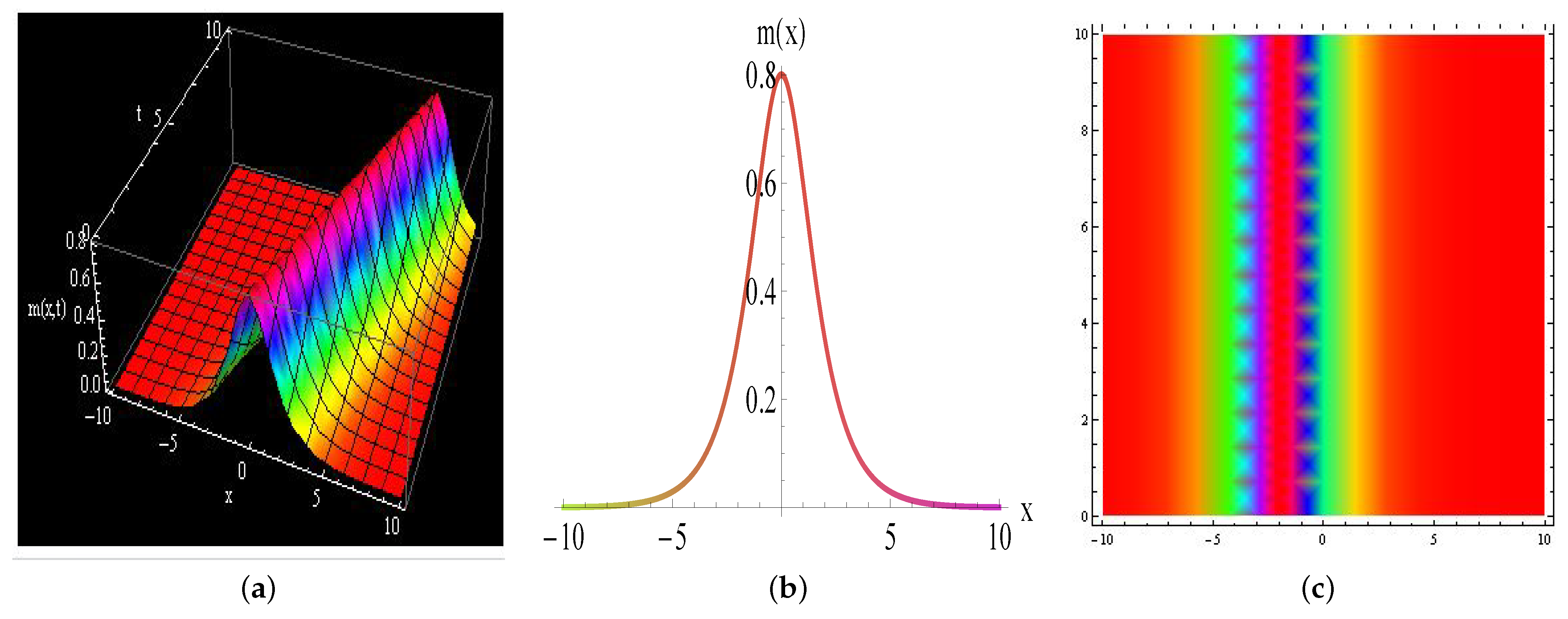
which represents a non-singular, localized single-soliton. The following figures show the one-soliton solution in contour, two-dimensional, and three-dimensional views.

4.2. Two-Soliton Solution

With the seed solution m = 0 , the second iteration m [ 2 ] can now be represented as follows:
m [ 2 ] = ι d d x ln ( L 1 ( X s , Y s ) [ 2 ] L 2 ( X s , Y s ) [ 2 ] ) ,
we can calculate the value for X 1 , Y 1 , X 2 and Y 2 from the linear system (12) at λ = λ 1 = ι k 1 and λ = λ 2 = ι k 2 respectively as below:
X 1 = cosh ( k 1 x 4 k 1 3 t ) + ι sinh ( k 1 x 4 k 1 3 t ) , Y 1 = cosh ( k 1 x 4 k 1 3 t ) ι sinh ( k 1 x 4 k 1 3 t ) ,
X 2 = cosh ( k 2 x 4 k 2 3 t ) + ι sinh ( k 2 x 4 k 2 3 t ) , Y 2 = cosh ( k 2 x 4 k 2 3 t ) ι sinh ( k x 4 k 2 3 t ) ,
so Equation (56) can be written as, which shows the two-soliton solution:
m [ 2 ] = 2 k 1 sinh ( k 1 x 4 k 1 3 t ) cosh ( k 2 x 4 k 2 3 t ) + k 2 sinh ( k 2 x 4 k 2 3 t ) cosh ( k 1 x 4 k 1 3 t ) cosh 2 ( k 1 x 4 k 1 3 t ) + cosh 2 ( k 2 x 4 k 2 3 t ) + 2 sinh ( k 1 x 4 k 1 3 t ) sinh ( k 2 x 4 k 2 3 t ) .
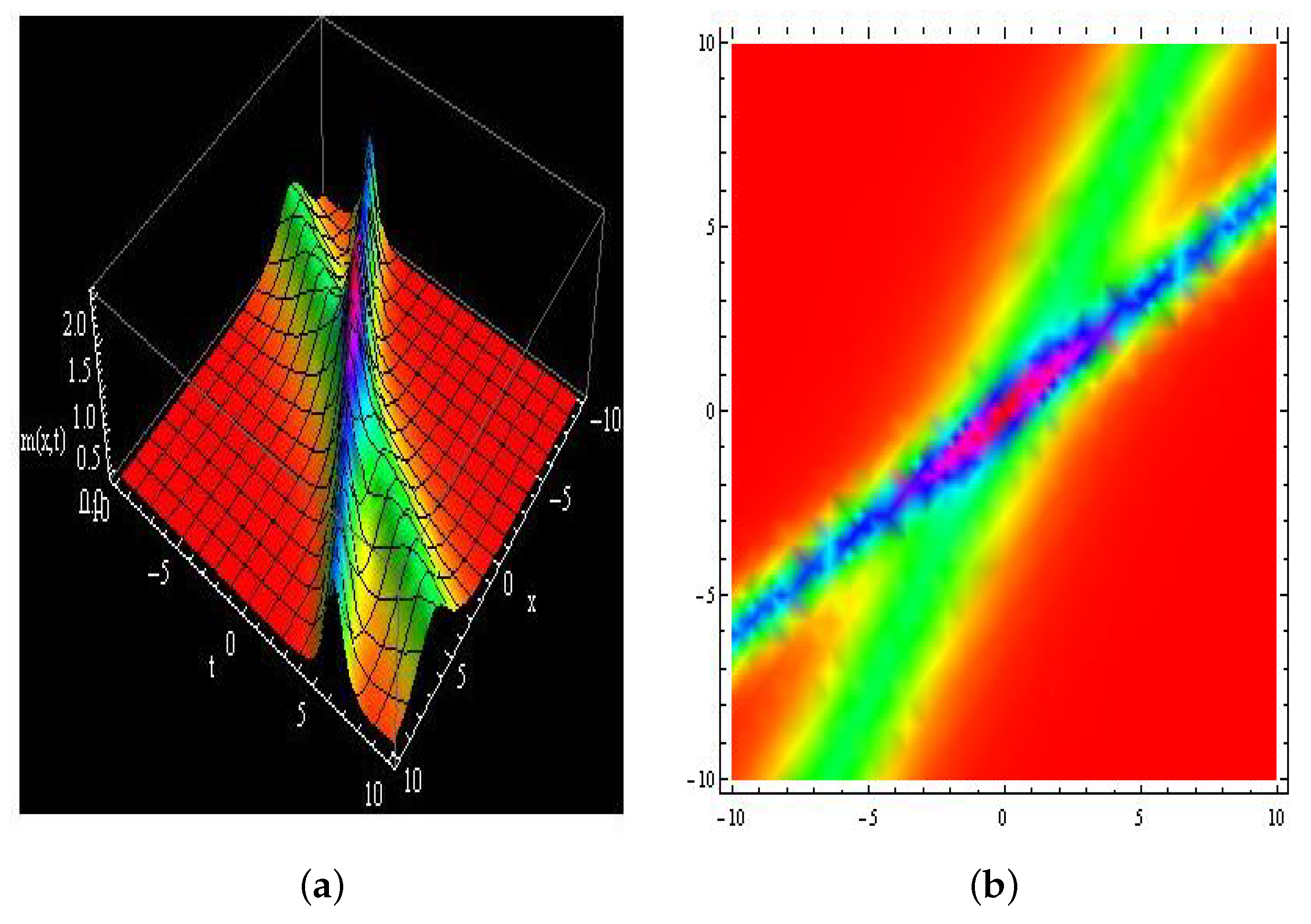
The following graphics illustrate the two-soliton solution in two-dimensional, three-dimensional, and contour representations.

4.3. Three-Soliton Solution

For the trivial initial solution m = 0 , the three-fold Darboux transformation (40) reduces to the following form:
m [ 3 ] = 1 ι d d x ln ( L 1 ( X s , Y s ) [ 3 ] L 2 ( X s , Y s ) [ 3 ] ) ,
the value of X 3 , Y 3 can be determined from system (12) by evaluating it at λ = λ 3 as follows:
X 3 = cosh ( k 3 x 4 k 3 3 t ) + ι sinh ( k 3 x 4 k 3 3 t ) , Y 3 = cosh ( k 3 x 4 k 3 3 t ) ι sinh ( k 3 x 4 k 3 3 t ) ,
substituting these values into Equation (60) and performing simplification, we have:
m [ 3 ] ( x , t ) = 1 i d d x ln H ( x , t ) I ( x , t ) ,
where:
χ 1 = k 1 x 4 k 1 3 t , χ 2 = k 2 x 4 k 2 3 t , χ 3 = k 3 x 4 k 3 3 t ,
and H ( x , t ) and I ( x , t ) are given as follows:
H ( x , t ) = cosh 2 ( χ 1 ) + cosh 2 ( χ 2 ) + cosh 2 ( χ 3 ) + ( k 1 k 2 ) 2 ( k 1 + k 2 ) 2 cosh 2 ( χ 1 + χ 2 ) + ( k 1 k 3 ) 2 ( k 1 + k 3 ) 2 cosh 2 ( χ 1 + χ 3 ) + ( k 2 k 3 ) 2 ( k 2 + k 3 ) 2 cosh 2 ( χ 2 + χ 3 ) + ( k 1 k 2 ) 2 ( k 1 k 3 ) 2 ( k 2 k 3 ) 2 ( k 1 + k 2 ) 2 ( k 1 + k 3 ) 2 ( k 2 + k 3 ) 2 cosh 2 ( χ 1 + χ 2 + χ 3 ) ,
I ( x , t ) = sinh 2 ( χ 1 ) + sinh 2 ( χ 2 ) + sinh 2 ( χ 3 ) + ( k 1 k 2 ) 2 ( k 1 + k 2 ) 2 sinh 2 ( χ 1 + χ 2 ) + ( k 1 k 3 ) 2 ( k 1 + k 3 ) 2 sinh 2 ( χ 1 + χ 3 ) + ( k 2 k 3 ) 2 ( k 2 + k 3 ) 2 sinh 2 ( χ 2 + χ 3 ) + ( k 1 k 2 ) 2 ( k 1 k 3 ) 2 ( k 2 k 3 ) 2 ( k 1 + k 2 ) 2 ( k 1 + k 3 ) 2 ( k 2 + k 3 ) 2 sinh 2 ( χ 1 + χ 2 + χ 3 ) ,
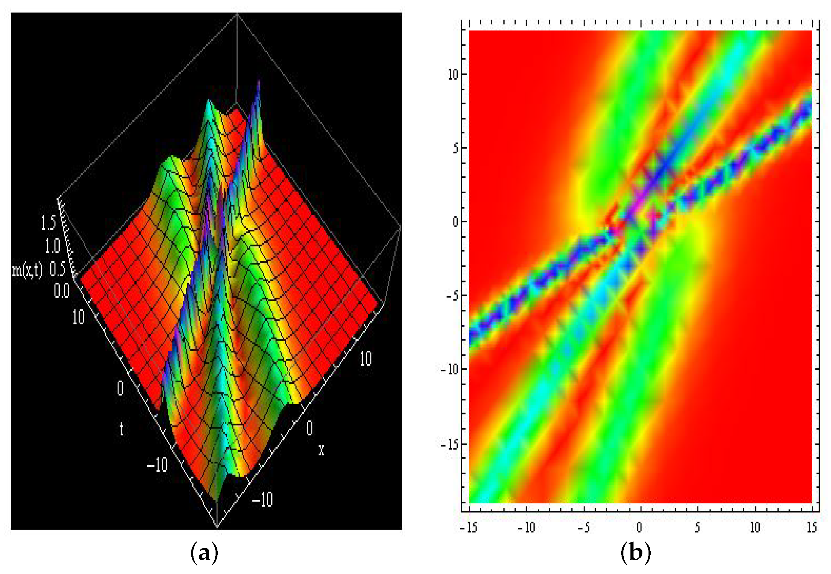
The explicit three-soliton solution for m corresponding to the combined KdV–mKdV equation is presented, along with the interactions between these solitons as illustrated below.
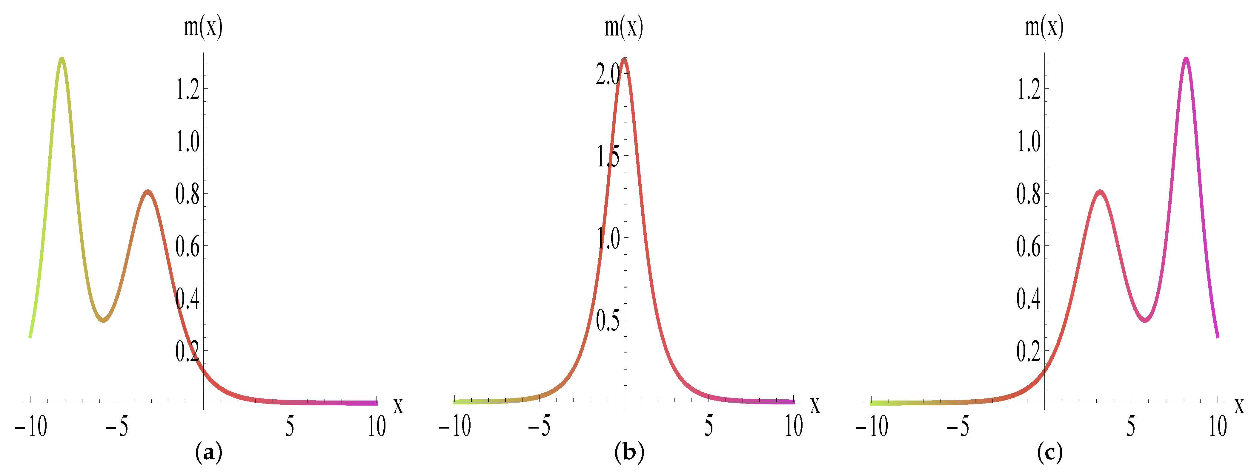
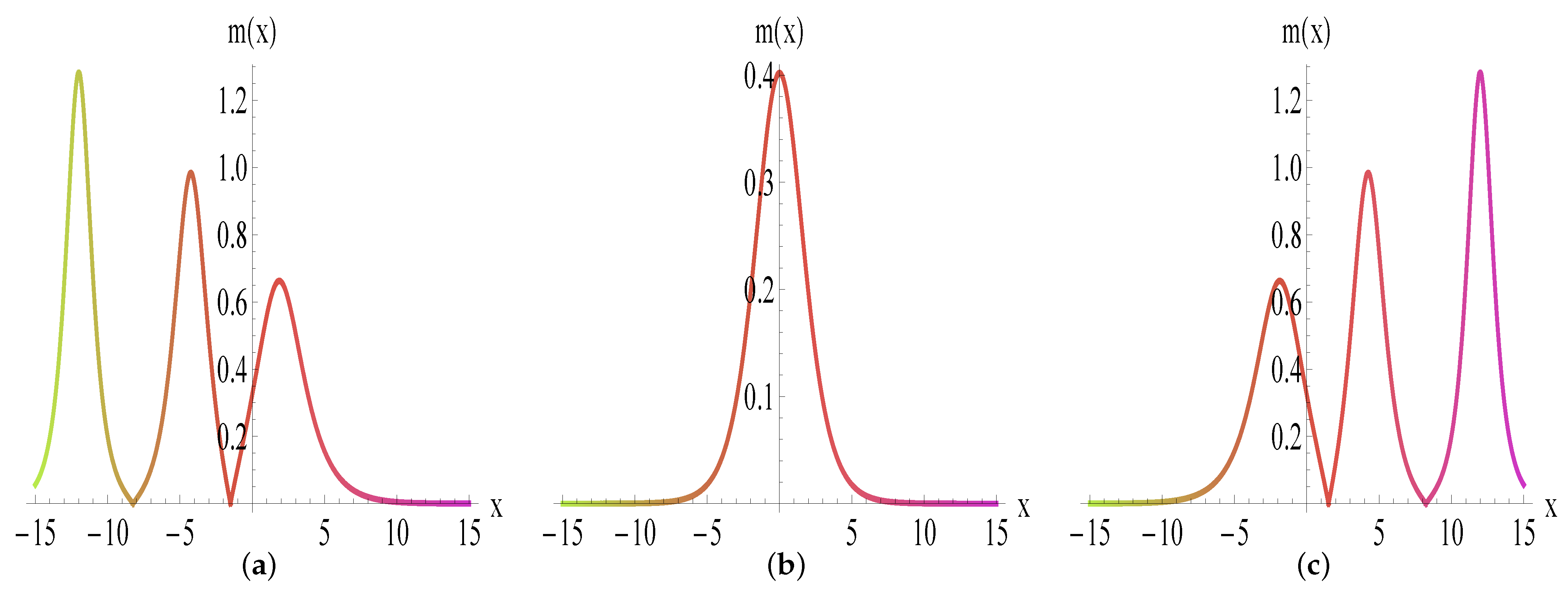
The one-soliton solution is shown in Figure 1, where the solitary wave’s amplitude, velocity, and localization are all controlled by the parameter k 1 . Figure 2 depicts the two-soliton solution, highlighting their nonlinear interaction as defined by parameters k 1 and k 2 . Figure 3, which depicts the solitons prior to, during, and following contact, highlights the elastic character of this interaction: aside from a phase shift, they briefly overlap before reemerging with their original forms and velocities. The three-soliton solution with parameters k 1 , k 2 , and k 3 is shown in Figure 4 and Figure 5, which demonstrate the resilience and the distinctive soliton trait of form preservation by displaying more intricate but still elastic interactions.

5. Multi-Wave and Periodic Cross-Kink Solutions

In this section, we present multi-wave and periodic cross-kink solutions. In order to derive these solution classes, the corresponding ordinary differential equation and its bilinear form must be created. To achieve the ordinary form of Equation (1), we employ the following ansatz into that equation [34].
m ( x , t ) = M ( ξ ) , ξ = x c t ,
where M is a scaling parameter and c denotes the wave velocity. By applying the traveling wave transformation given in Equation (66) to Equation (1), we arrive at the following reduced equation.
M c M 3 M 2 + 2 a M 3 = 0 .
The bilinear form [35] is constructed via the following transformation, implying the computation of different kinds of its solitary wave solutions:
M = 2 ( log f ) ξ ,
substituting Equation (68) into Equation (67) yields the corresponding bilinear form:
16 a f ξ 3 2 c f 2 f ξ + 4 f ξ 3 + 2 f 2 f ξ ξ ξ 6 f ξ ξ ( f f ξ ) 12 ( f f ξ ) 2 = 0 .

5.1. Multi-Wave Solution

In this section, the multi-wave solution is constructed [36], which combines trigonometric and hyperbolic functions, allowing the representation of both solitary and periodic wave structures in a unified form. To obtain these solutions, the following transformations are employed [37]:
f = k 0 cosh ( a 1 ξ + a 2 ) + k 1 cos ( a 3 ξ + a 4 ) + k 2 cosh ( a 5 ξ + a 6 ) ,
where k i ( i = 0 , 1 , 2 ) and a i ( 1 i 6 ) are real parameters. Inserting f into Equation (69) and collecting all the terms involving cos 2 ( a 4 + a 3 ξ ) sinh ( a 6 + a 5 ξ ) , cosh 2 ( a 2 + a 1 ξ ) sinh ( a 6 + a 5 ξ ) , cosh ( a 2 + a 1 ξ ) cosh ( a 6 + a 5 ξ ) sinh ( a 6 + a 5 ξ ) , etc, we obtain a system of equations that yields the following parameter values:
a 1 = i c 2 , a 3 = c 2 , a 4 = a 4 , k 2 = 0 , k 1 = k 1 ,
substituting these constants values in Equation (70), we get:
f = k 1 cos a 4 + c ξ 2 + k 0 cosh a 2 + i c ξ 2 ,
By inserting Equation (72) into Equation (68) and simplifying it, we obtain the expression as follows:
M = 2 c k 1 sin a 4 + c 2 ξ + i k 0 sinh a 2 + i c 2 ξ k 1 cos a 4 + c 2 ξ + k 0 cosh a 2 + i c 2 ξ
By inserting Equation (73) into Equation (66), we get the multi-wave solution of Equation (1):
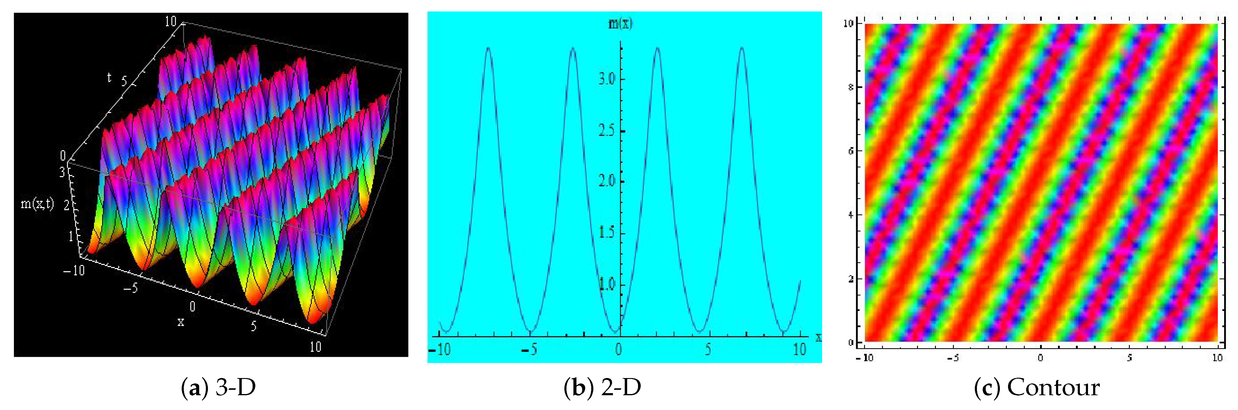
m = 2 c k 1 sin a 4 + c 2 ( x c t ) + i k 0 sinh a 2 + i c 2 ( x c t ) k 1 cos a 4 + c 2 ( x c t ) + k 0 cosh a 2 + i c 2 ( x c t ) .

5.2. Periodic Cross-Kink Wave Solution

In this section, we investigate the periodic cross-kink wave solution of the combined KdV-mKdV equation. This class of solutions is characterized by the interplay of hyperbolic, trigonometric, and exponential functions, supplemented with arbitrary coefficients that provide additional flexibility in shaping the wave profiles. To derive these solutions, we employ the transformation given below [36].
f = e ζ 1 + ζ 1 e ζ 1 + ζ 2 cos ( ζ 2 ) + ζ 3 cosh ( ζ 3 ) + d 7 , ζ 1 = d 1 ξ + d 2 , ζ 2 = d 3 ξ + d 4 , ζ 3 = d 5 ξ + d 6 ,
where d i ( 1 i 7 ) and ζ i ( i = 1 , 2 , 3 ) denote real parameters. By substituting the expression of f into Equation (69) and collecting all powers of e d 2 d 1 ξ ξ sinh 2 ( d 6 + d 5 ξ ) , e d 2 + d 1 ξ ξ sinh 2 ( d 6 + d 5 ξ ) , e d 2 + d 1 ξ ξ 2 sinh 2 ( d 6 + d 5 ξ ) , e d 2 + d 1 ξ ξ 3 sinh 2 ( d 6 + d 5 ξ ) , cos ( d 4 + d 3 ξ ) sinh 2 ( d 6 + d 5 ξ ) , e 3 d 2 3 d 1 ξ , e 2 d 2 2 d 1 ξ , ξ 3 sinh 3 ( d 6 + d 5 ξ ) , ξ 2 sinh 3 ( d 6 + d 5 ξ ) , ξ sinh 3 ( d 6 + d 5 ξ ) , sinh 3 ( d 6 + d 5 ξ ) , ξ 3 sin ( d 4 + d 3 ξ ) sinh 2 ( d 6 + d 5 ξ ) , and ξ 2 sin ( d 4 + d 3 ξ ) sinh 2 ( d 6 + d 5 ξ ) , etc., we obtain a set of algebraic equations that determine the values of the corresponding coefficients:
d 1 = 0 , d 2 = d 2 , d 3 = i c 3 , d 4 = d 4 , d 5 = 0 .
Using the values of unknown constants into Equation (75), we get the following form:
f = d 7 + e d 2 + d 2 e d 2 + d 4 i c ξ 3 cos d 4 i c ξ 3 + d 6 cosh ( d 6 ) + d 7 ,
By inserting Equation (77) into Equation (68), we get:
M = 2 i c cos d 4 i c ξ 3 d 4 i c ξ 3 sin d 4 i c ξ 3 3 d 7 + e d 2 + d 2 e d 2 + d 4 i c ξ 3 cos d 4 i c ξ 3 + d 6 cosh ( d 6 ) ,
By inserting Equation (78) into Equation (66), we obtain the periodic cross-kink wave solution associated with Equation (1):
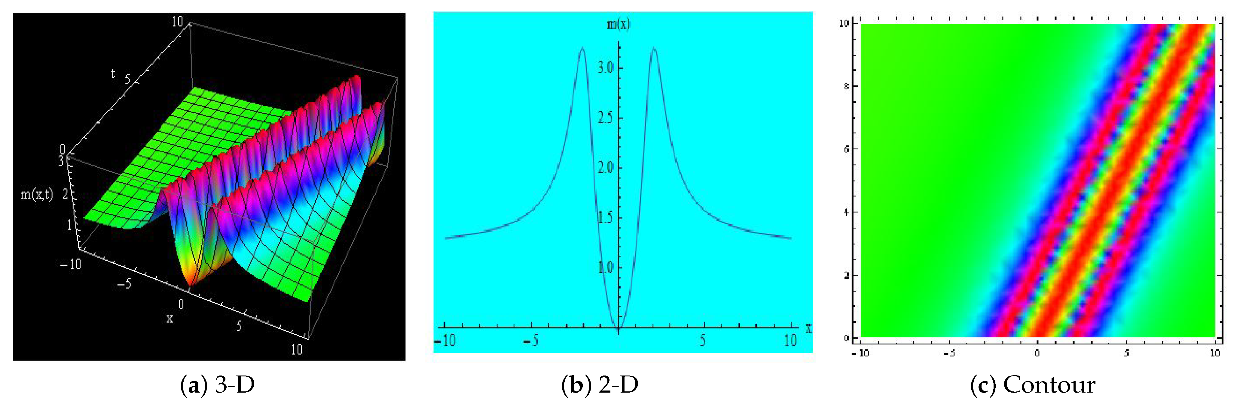
m = 2 i c cos d 4 i c ( c t + x ) 3 d 4 i c ( c t + x ) 3 sin d 4 i c ( c t + x ) 3 3 d 7 + e d 2 + d 2 e d 2 + d 4 i c ( c t + x ) 3 cos d 4 i c ( c t + x ) 3 + d 6 cosh ( d 6 ) .
Figure 6 and Figure 7 show the multi-wave and periodic cross-kink wave solutions. Unlike classical soliton solutions, these multi-wave and cross-kink structures arise from mixed hyperbolic-trigonometric forms in the bilinear representation, leading to more complex wave interactions. The modeling of intricate physical processes like energy localization and nonlinear wave interactions is greatly aided by these kinds of solutions. Such solutions are important for understanding wave propagation, pattern formation, and nonlinear excitations in systems like optical fibers, plasmas, and spin chains.

6. Conclusions

One of the paper’s key findings is the computational realization of the K-fold Darboux transformation for the combined KdV-mKdV model into Wronskians, which enables the development of multi-soliton solutions inside the Darboux framework. Figure 1, Figure 2, Figure 3, Figure 4 and Figure 5 provide exact solutions for one-, two-, and three-soliton profiles that highlight the practical and computational aspects of our approach. In addition, multi-wave and periodic cross-kink solutions to the combined KdV-mKdV model are generated, along with graphical representations for various parameter values. Our long-term goal is to build an algebraic Bäcklund transformation with a quadrilateral structure using the Darboux transformation. The formation of multi-soliton solutions in unique expressions with a collection of solitary wave solutions provides an alternative algebraic construction of the combined KdV-mKdV problem. The Darboux solutions described here provide a future impetus to examine the non-commutative analog of the combined KdV-mKdV model extension, as well as its quasideterminant solutions, which will be discussed in another paper. This extension may recover the results reported here in the commutative limit while also providing a broader grasp of the combined KdV-mKdV model’s integrability and advanced applications.

Author Contributions

Conceptualization, I.M.; Methodology, N.R. and E.H.; Software, N.R. and E.H.; Validation, I.M.; Investigation, N.R.; Resources, R.A.A.; Data curation, I.M.; Writing—original draft, N.R. and E.H.; Writing—review & editing, R.A.A. and E.H.; Supervision, I.M.; Project administration, R.A.A.; Funding acquisition, R.A.A. All authors have read and agreed to the published version of the manuscript.

Funding

This work was supported and funded by the Deanship of Scientific Research at Imam Mohammad Ibn Saud Islamic University (IMSIU) (grant number IMSIU-DDRSP2602).

Data Availability Statement

This study was not supported by newly created or examined data.

Conflicts of Interest

The authors declare no conflicts of interest.

References

  1. Ablowitz, M.J.; Clarkson, P.A. Solitons, Nonlinear Evolution Equations and Inverse Scattering; Cambridge University Press: Cambridge, UK, 1992. [Google Scholar]
  2. Lou, S.Y.; Tang, X.Y. Nonlinear Mathematical Physics Methods; Science Press: Beijing, China, 2006. (In Chinese) [Google Scholar]
  3. Malik, S.; Hashemi, M.S.; Kumar, S.; Rezazadeh, H.; Mahmoud, W.; Osman, M.S. Application of new Kudryashov method to various nonlinear partial differential equations. Opt. Quantum Electron. 2023, 55, 8. [Google Scholar] [CrossRef] [Scilit]
  4. Lin, Z.; Wen, X.Y. Hodograph transformation, various exact solutions and dynamical analysis for the complex Wadati-Konno-Ichikawa-II equation. Phys. D Nonlinear Phenom. 2023, 451, 133770. [Google Scholar] [CrossRef] [Scilit]
  5. Abdulwahhab, M.A. Comment on “Lie symmetry analysis, optimal system, new solitary wave solutions and conservation laws of the Pavlov equation’’ by Nardjess Benoudina and et al. [CNSNS 2021, 94: 105560]. Commun. Nonlinear Sci. Numer. Simul. 2021, 101, 105868. [Google Scholar] [CrossRef] [Scilit]
  6. Ali, A.; Ahmad, J.; Javed, S. Dynamic investigation to the generalized Yu–Toda–Sasa–Fukuyama equation using Darboux transformation. Opt. Quantum Electron. 2024, 56, 166. [Google Scholar] [CrossRef] [Scilit]
  7. Zabusky, N.J.; Galvin, C.J. Shallow-water waves, the Korteweg-deVries equation and solitons. J. Fluid Mech. 1971, 47, 811–824. [Google Scholar] [CrossRef] [Scilit]
  8. Khater, A.H.; Callebaut, D.K.; Seadawy, A.R. General soliton solutions for nonlinear dispersive waves in convective type instabilities. Phys. Scr. 2006, 74, 384. [Google Scholar] [CrossRef] [Scilit]
  9. Kartashov, Y.V.; Malomed, B.A.; Torner, L. Solitons in nonlinear lattices. Rev. Mod. Phys. 2011, 83, 247–305. [Google Scholar] [CrossRef] [Scilit]
  10. Wang, D.S.; Zhang, X.F.; Zhang, P.; Liu, W.M. Matter-wave solitons of Bose–Einstein condensates in a time-dependent complicated potential. J. Phys. B At. Mol. Opt. Phys. 2009, 42, 245303. [Google Scholar] [CrossRef] [Scilit]
  11. Wang, D.S.; Song, S.W.; Xiong, B.; Liu, W.M. Quantized vortices in a rotating Bose-Einstein condensate with spatiotemporally modulated interaction. Phys. Rev. A—Atomic Mol. Opt. Phys. 2011, 84, 053607. [Google Scholar] [CrossRef] [Scilit]
  12. Kartashov, Y.V.; Vysloukh, V.A.; Torner, L. Surface gap solitons. Phys. Rev. Lett. 2006, 96, 073901. [Google Scholar] [CrossRef] [Scilit] [PubMed]
  13. Zhao, W.; Huang, L. The optical solitons for the three-component Dirac–Manakov system via the Darboux transformation. Opt. Quant. Electron. 2024, 56, 1113. [Google Scholar] [CrossRef] [Scilit]
  14. Miura, R.M. Bäcklund Transformations, the Inverse Scattering Method, Solitons, and Their Applications: NSF Research Workshop on Contact Transformations; Springer: Berlin/Heidelberg, Germany, 1976. [Google Scholar]
  15. Ablowitz, M.J.; Kaup, D.J.; Newell, A.C.; Segur, H. The inverse scattering transformation Fourier analysis for nonlinear problems. Stud. Appl. Math. 1974, 53, 249–315. [Google Scholar] [CrossRef] [Scilit]
  16. Zhang, G.Q.; Yan, Z.Y.; Wen, X.Y.; Chen, Y. Interactions of localized wave structures and dynamics in the defocusing coupled nonlinear Schrödinger equations. Phys. Rev. E 2017, 95, 042201. [Google Scholar] [CrossRef] [Scilit] [PubMed]
  17. Zhang, Y.; Yang, J.W.; Chow, K.W.; Wu, C.F. Solitons, breathers and rogue waves for the coupled Fokas–Lenells system via Darboux transformation. Nonlinear Anal. Real World Appl. 2017, 33, 237–252. [Google Scholar] [CrossRef] [Scilit]
  18. Xu, S.W.; He, J.S.; Wang, L.H. The Darboux transformation of the derivative nonlinear Schrödinger equation. J. Phys. A Math. Theor. 2011, 44, 305203–305225. [Google Scholar] [CrossRef] [Scilit]
  19. Lv, N.N.; Huang, L. Breather-soliton molecules and breather-positons for the extended complex modified KdV equation. Commun. Nonlinear Sci. Numer. Simul. 2022, 107, 106148. [Google Scholar] [CrossRef] [Scilit]
  20. Berjawi, M.; Arwadi, T.E.; Israwi, S. A well-posedness result for an extended kdv equation. Partial. Differ. Equ. Appl. Math. 2024, 10, 100715. [Google Scholar] [CrossRef] [Scilit]
  21. Kaya, D.; İnan, I.E. A numerical application of the decomposition method for the combined KdV–MKdV equation. Appl. Math. Comput. 2005, 168, 915–926. [Google Scholar] [CrossRef] [Scilit]
  22. Yuan, R.R.; Shi, Y.; Zhao, S.L.; Zhao, J.X. The combined KdV-mKdV equation: Bilinear approach and rational solutions with free multi-parameters. Results Phys. 2023, 55, 107188. [Google Scholar] [CrossRef] [Scilit]
  23. Mohamad, M.N.B. Exact solutions to the combined KdV and mKdV equation. Math. Methods Appl. Sci. 1992, 15, 73–78. [Google Scholar] [CrossRef] [Scilit]
  24. Matveev, V.B.; Salle, M.A. Darboux Transformations and Solitons; Springer Series in Nonlinear Dynamics; Springer: Berlin/Heidelberg, Germany, 1991. [Google Scholar]
  25. Gu, C.; Hu, H.; Zhou, Z. Darboux Transformations in Integrable Systems: Theory and Their Applications to Geometry; Springer Science & Business Media: Berlin/Heidelberg, Germany, 2004. [Google Scholar]
  26. Trisetyarso, A. Application of Darboux Transformation to solve Multisoliton Solution on Non-linear Schrödinger Equation. arXiv 2009, arXiv:0910.0901. [Google Scholar]
  27. Trisetyarso, A. Correlation of Dirac potentials and atomic inversion in cavity quantum electrodynamics. J. Math. Phys. 2010, 51, 072103. [Google Scholar] [CrossRef] [Scilit]
  28. Trisetyarso, A. Dirac four-potential tunings-based quantum transistor utilizing the Lorentz force. arXiv 2010, arXiv:1003.4590. [Google Scholar] [CrossRef] [Scilit]
  29. Li, C.X.; Nimmo, J.J.C. Darboux transformations for a twisted derivation and quasideterminant solutions to the super kdv equation. Proc. R. Soc. A Math. Phys. Eng. Sci. 2010, 466, 2471–2493. [Google Scholar] [CrossRef] [Scilit]
  30. Zhang, J.; Cui, W.; Wang, H. Quasi-periodic solutions of a non-autonomous kdv-mkdv equation with periodic unbounded conditions. J. Comb. Math. Comb. Comput. 2025, 127, 7113–7139. [Google Scholar]
  31. Mahmood, I.; Li, Z.; Sohail, H.; Ditta, A.; Elansary, H.O.; Hussain, E. Multi-soliton solutions of ito-type coupled kdv equation with conservation laws in darboux framework. Int. J. Geom. Methods Mod. Phys. 2024, 21, 2450205. [Google Scholar] [CrossRef] [Scilit]
  32. Irfan, M. Lax pair representation and darboux transformation of noncommutative painlevé’s second equation. J. Geom. Phys. 2012, 62, 1575–1582. [Google Scholar] [CrossRef] [Scilit]
  33. Waseem, M.; Mahmood, I.; Sohail, H.; Hussain, E.; Elansary, H.O. Quantum painlevé second lax pair and quantum (matrix) analogues of classical painlevé ii equation. J. Phys. Soc. Jpn. 2024, 93, 054001. [Google Scholar] [CrossRef] [Scilit]
  34. Hussain, E.; Tedjani, A.H.; Murad, M.A.S. Exploring nonlinear dynamics of the (3+ 1)-dimensional boussinesq-type equation: Wave patterns and sensitivity insight. Axioms 2026, 15, 198. [Google Scholar] [CrossRef] [Scilit]
  35. Yang, J.Y.; Ma, W.X.; Qin, Z. Lump and lump-soliton solutions to the (2+1)-dimensional ito equation. Anal. Math. Phys. 2018, 8, 427–436. [Google Scholar] [CrossRef] [Scilit]
  36. Seadawy, A.R.; Younis, M.; Althobaiti, A. Various forms of m-shaped rational, periodic cross kink waves and breathers for bose-einstien condensate model. Opt. Quantum Electron. 2022, 54, 152. [Google Scholar] [CrossRef] [Scilit]
  37. Raees, N.; Tedjani, A.H.; Mahmood, I.; Hussain, E. Diversity of optical soliton solutions of akbota models in the application of heisenberg ferromagnet. Symmetry 2025, 17, 2149. [Google Scholar] [CrossRef] [Scilit]
Figure 1. For k 1 = 0.4 (a) 3-D profile of one-soliton solution. (b) 2-D profile of one-soliton solution. (c) Contour representation of one-soliton solution.
Mathematics 14 01488 g001
Figure 2. For k 1 = 0.4, k 2 = 0.64. (a) 3-D perspective of a two-soliton. (b) Contour representation of the two-soliton solution.
Mathematics 14 01488 g002
Figure 3. (a) 2-D profile of two-soliton before interaction ( t < 0). (b) 2-D profile of a two-soliton during interaction (t = 0). (c) 2-D profile of a two-soliton after interaction ( t > 0).
Mathematics 14 01488 g003
Figure 4. For k 1 = 0.4, k 2 = 0.64, k 3 = 0.35. (a) 3-D perspective of a three-soliton. (b) Contour representation of the three-soliton solution.
Mathematics 14 01488 g004
Figure 5. (a) 2-D profile of three-soliton before interaction ( t < 0). (b) 2-D profile of three-soliton during interaction (t = 0). (c) 2-D profile of three-soliton after interaction ( t > 0).
Mathematics 14 01488 g005
Figure 6. Represents the 3-D, 2-D and contour plot of Equation (74) for c = 0.9 , k 1 = 0.6 , a 4 = 0.4, a 2 = 0.8, and k 0 = 0.7.
Mathematics 14 01488 g006
Figure 7. Represents the 3-D, 2-D and contour plot of Equation (79) for c = 0.9 , d 4 = 0.6 , d 6 = 0.5 , d 2 = 0.3 , and d 7 = 0.2 .
Mathematics 14 01488 g007
Disclaimer/Publisher’s Note: The statements, opinions and data contained in all publications are solely those of the individual author(s) and contributor(s) and not of MDPI and/or the editor(s). MDPI and/or the editor(s) disclaim responsibility for any injury to people or property resulting from any ideas, methods, instructions or products referred to in the content.