Pseudodifferential Phase-Space Dynamics for SU(1,1) Systems and Numerical Evaluation Using Oscillatory Integrals

Abstract

We study the phase-space dynamics of quantum systems with $\mathrm{SU}(1,1)$ group symmetry using coherent-state representations on the Poincaré disk. The resulting evolution equation combines transport terms with nonlocal contributions generated with the spectral functions of the Casimir operator, which admit a natural interpretation as pseudodifferential operators associated with the hyperbolic Laplace–Beltrami operator. Using this pseudodifferential structure, we classify the phase-space generators according to the type of the underlying PDE: compact quadratic dynamics ($\widehat{H}\propto {\widehat{K}}_0^2$) yield a degenerate hyperbolic operator of the transport type, and noncompact dynamics ($\widehat{H}\propto {\widehat{K}}_2^2$) give rise to a mixed-order differential–pseudodifferential operator. For numerical evaluation, we reformulate the propagator as an oscillatory integral and develop two complementary strategies: a Fourier-series reduction exploiting the periodicity of compact orbits and a Levin-type spectral collocation method for the noncompact case. Both approaches are stable, accurate, and free of the stiffness issues that afflict direct PDE evolution on the Poincaré disk.

1. Introduction

Quantum systems possessing $\mathrm{SU}(1,1)$ group symmetry arise in a variety of physical contexts, including quantum optics, parametric amplification, and squeezed states [1,2,3,4,5,6]. Phase-space methods [7,8] provide a powerful framework for analyzing these systems by representing quantum states as functions on the curved phase space associated with the coherent-state manifold, which for $\mathrm{SU}(1,1)$ is the Poincaré disk [9].

Although numerical methods for phase-space dynamics are well-developed for systems with other relevant symmetries, such as the Heisenberg–Weyl and $\mathrm{SU}\left(2\right)$ groups, the corresponding literature for $\mathrm{SU}(1,1)$ group remains comparatively limited. In the canonical (Heisenberg–Weyl) setting, a broad range of techniques have been established for the numerical evolution of quasiprobability distributions, including deterministic and stochastic methods [10,11,12,13]. Similarly, for $\mathrm{SU}\left(2\right)$ systems, phase-space methods on the sphere have been extensively developed, with numerical schemes exploiting spherical harmonic expansions, discrete representations, and semiclassical approximations [14,15,16].

In contrast, only recently has a formal phase-space description of quantum systems with $\mathrm{SU}(1,1)$ group symmetry been developed [17], and explicit differential representations for the action of the generators on the corresponding phase-space functions have subsequently been derived [18,19,20]. However, systematic and efficient numerical methods for the evolution of quasidistributions on a hyperbolic disk remain limited.

In particular, the dynamics generated by quadratic Hamiltonians, which arise in several physically relevant settings [21,22,23,24], lead to evolution equations that combine transport behavior with nonlocal corrections induced by the Casimir operator of Lie algebra [19]. Understanding the structure of these equations requires tools from representation theory, differential geometry, and pseudodifferential analysis of manifolds, and their numerical treatment poses significant analytical and computational challenges.

In this setting, this work has two goals. First, we analyze the mathematical structure of the evolution equations and show that they can be interpreted as transport-type equations with pseudodifferential corrections on the hyperbolic disk; we further classify the resulting PDEs by type, identifying regimes of degenerate hyperbolic and mixed-order behavior. Second, in order to overcome the difficulties posed by the direct phase-space evolution equation, we develop an alternative strategy for evaluating the evolution of the phase-space function by means of an oscillatory propagator, which we compute using suitable numerical methods for highly oscillatory integrals [25,26].

This paper is organized as follows: Section 2 introduces the phase-space representation of $\mathrm{SU}(1,1)$ and the geometric form of the Casimir operator. Section 3 analyzes the pseudodifferential structure of the compact and noncompact quadratic generators. Section 4 presents the two numerical strategies and their validation. Section 5 summarizes the main results.

2. Phase-Space Representation

Let ${\widehat{K}}_0,{\widehat{K}}_1,{\widehat{K}}_2$ denote the generators of $\mathfrak{su}(1,1)$ algebra, satisfying

$$[{\widehat{K}}_0,{\widehat{K}}_1]=i{\widehat{K}}_2,[{\widehat{K}}_0,{\widehat{K}}_2]=-i{\widehat{K}}_1,[{\widehat{K}}_1,{\widehat{K}}_2]=-i{\widehat{K}}_0.$$

(1)

The Casimir operator is

$$J^2={\widehat{K}}_0^2-{\widehat{K}}_1^2-{\widehat{K}}_2^2.$$

(2)

For discrete series representations, labeled by the Bargmann index $k={\displaystyle \frac{1}{2}},1,{\displaystyle \frac{3}{2}},\dots$ [27], the generators admit a phase-space (D algebra [28]) realization as differential operators acting on functions on the Poincaré disk $\mathbb{D}=\{\zeta \in \mathbb{C}:|\zeta |<1\}$ [29].

This space can be identified with symmetric space $\mathrm{SU}(1,1)/\mathrm{U}\left(1\right)$ and has a natural invariant hyperbolic geometry. As a consequence, the Casimir operator admits a geometric realization in terms of the Laplace–Beltrami operator, which provides the key link between representation theory and pseudodifferential analysis [30,31].

Definition 1. 

The phase-space Casimir operator is

$${\mathcal{K}}^2={\mathcal{K}}_0^2-{\mathcal{K}}_1^2-{\mathcal{K}}_2^2,$$

(3)

acting on phase-space functions $W\left(\zeta \right)$.

Remark 1. 

The operators $J^2$ and ${\mathcal{K}}^2$ represent the same Casimir element of the universal enveloping algebra of $\mathfrak{su}(1,1)$ in different realizations: $J^2$ acts on the Hilbert space of the representation, while ${\mathcal{K}}^2$ is its phase-space counterpart obtained via D-algebra mapping. In particular, both operators share the same spectrum, and the D-algebra construction intertwines their functional calculi.

Introducing hyperbolic coordinates

$$\zeta =tanh\left({\displaystyle \frac{\tau }{2}}\right)e^{-i\varphi },\tau \ge 0,\varphi \in [0,2\pi ),$$

(4)

the phase-space Casimir operator takes the explicit form [32]

$${\mathcal{K}}^2=-\left({\partial }_{\tau }^2+coth\tau {\partial }_{\tau }+{\displaystyle \frac{1}{{sinh}^2\tau }}{\partial }_{\varphi }^2\right).$$

(5)

This is the content of the following lemma, which is used throughout; its proof is provided in Appendix A.

Lemma 1 

(Casimir as Laplace–Beltrami operator). In hyperbolic coordinates $(\tau ,\varphi )$, the phase-space Casimir operator coincides (up to sign convention) with the Laplace–Beltrami operator on a hyperbolic disk:

$${\mathcal{K}}^2=-{\Delta }_{\mathbb{H}}.$$

(6)

Its principal symbol is

$$p_h(\tau ,\varphi ;{\xi }_{\tau },{\xi }_{\varphi })={\xi }_{\tau }^2+{\displaystyle \frac{{\xi }_{\varphi }^2}{{sinh}^2\tau }},$$

(7)

so ${\mathcal{K}}^2$ is an elliptic operator of order two. The principal symbol $p_h$ characterizes the order of any spectral function $\Phi \left({\mathcal{K}}^2\right)$ and determines whether such functions define elliptic pseudodifferential operators.

3. Pseudodifferential Structure of $\mathrm{SU}(\mathbf{1},\mathbf{1})$ Phase-Space Equations

The geometric representation un Section 2 allows one to interpret the spectral functions of the Casimir operator within the framework of the pseudodifferential analysis of manifolds. A key structural distinction between the compact and noncompact generators is already apparent at the level of the principal symbol: the former leads to a degenerate hyperbolic (transport-type) operator characterized by angular advection with nonlocal radial dependence, while the latter gives rise to a nonelliptic operator of the mixed type, involving a coupled first- and second-order differential–pseudodifferential structure. The following propositions make this precise; their proofs are outlined in Appendix A.

The next result establishes the connection between the spectral functional calculus of the Casimir operator and its geometric realization on the hyperbolic disk.

Proposition 1 

(Pseudodifferential interpretation of Casimir multipliers). Let Φ be a smooth function. Then, in the sense of pseudodifferential calculus on manifolds, the operator $\Phi \left({\mathcal{K}}^2\right)$ is a pseudodifferential operator whose principal symbol is

$${\sigma }_{\mathrm{pr}}(\Phi \left({\mathcal{K}}^2\right))=\Phi \left(p_h\right).$$

(8)

If Φ is elliptic on the spectrum of ${\mathcal{K}}^2$, then $\Phi \left({\mathcal{K}}^2\right)$ is elliptic, and its inverse satisfies

$${\sigma }_{\mathrm{pr}}\left({\Phi }^{-1}\left({\mathcal{K}}^2\right)\right)=\Phi {\left(p_h\right)}^{-1}.$$

(9)

This result provides the key tool for identifying the order and ellipticity properties of the operators appearing in the phase-space evolution equations through their principal symbols.

3.1. Compact Quadratic Dynamics: $\widehat{H}\propto {\widehat{K}}_0^2$

The Wigner function evolves according to [19]

$$\begin{array}{cc}i{\partial }_{t}W(\zeta ,t)\hfill & =-[{\displaystyle \frac{1+{\left|\zeta \right|}^2}{1-{\left|\zeta \right|}^2}}(\zeta {\partial }_{\zeta }-{\zeta }^{*}{\partial }_{{\zeta }^{*}})\left(\frac{1}{2ϵ}\Phi \left({\mathcal{K}}^2\right)-\frac{ϵ}{2}{\Phi }^{-1}\left({\mathcal{K}}^2\right)\right)\hfill \\ \hfill & -ϵ\left(\zeta {\partial }_{\zeta }-{\zeta }^{*}{\partial }_{{\zeta }^{*}}+{\zeta }^2{\partial }_{\zeta }^2-{\zeta }^{*2}{\partial }_{{\zeta }^{*}}^2\right){\Phi }^{-1}\left({\mathcal{K}}^2\right)]W(\zeta ,t),\hfill \end{array}$$

(10)

where $ϵ={(2k-1)}^{-1}$, and $\zeta$ is given in Equation (4).

Using the identities

$$\zeta {\partial }_{\zeta }-{\zeta }^{*}{\partial }_{{\zeta }^{*}}=i{\partial }_{\varphi },{\displaystyle \frac{1+{\left|\zeta \right|}^2}{1-{\left|\zeta \right|}^2}}=cosh\tau ,$$

(11)

the evolution equation takes the form

$${\partial }_{t}W(\tau ,\varphi ,t)=-{\mathcal{L}}_{0}W(\tau ,\varphi ,t),{\mathcal{L}}_0=\mathcal{A}(\tau ,{\partial }_{\tau },{\mathcal{K}}^2){\partial }_{\varphi },$$

(12)

where $\mathcal{A}$ is a differential–pseudodifferential operator.

Within this framework, we now characterize the PDE type of the compact quadratic generator at the level of its principal symbol.

Proposition 2 

(Compact dynamics: degenerate hyperbolic structure). The generator ${\mathcal{L}}_0$ is nonelliptic. Its principal symbol is

$$\sigma \left({\mathcal{L}}_0\right)=-i{\xi }_{\varphi }cosh\tau \left(\frac{1}{2ϵ}\Phi \left(p_h\right)-\frac{ϵ}{2}{\Phi }^{-1}\left(p_h\right)\right)+ϵsinh\tau {\xi }_{\tau }{\xi }_{\varphi }{\Phi }^{-1}\left(p_h\right),$$

(13)

which vanishes when ${\xi }_{\varphi }=0$. Consequently, ${\mathcal{L}}_0$ is a degenerate operator: characteristics exist in the angular direction, and the evolution is of the transport type in ϕ, with nonlocal radial corrections encoded by $\Phi \left({\mathcal{K}}^2\right)$.

The evolution is driven by angular transport, while the radial dependence enters through nonlocal pseudodifferential coefficients. The degeneracy reflects the lack of ellipticity and the absence of regularizing effects.

3.2. Noncompact Quadratic Dynamics: $\widehat{H}\propto {\widehat{K}}_2^2$

The evolution equation reads [19]

$${\partial }_{t}W(\zeta ,t)={\mathcal{L}}_{2}W(\zeta ,t),{\mathcal{L}}_2={\mathcal{X}}_2{\mathcal{M}}_1\left({\mathcal{K}}^2\right)+{\mathcal{Y}}_2{\mathcal{M}}_2\left({\mathcal{K}}^2\right),$$

(14)

where ${\mathcal{X}}_2$ is a first-order and ${\mathcal{Y}}_2$ is a second-order differential operator arising from the D-algebra realization of ${\widehat{K}}_2$ (see Appendix A.4), and the spectral multipliers are

$${\mathcal{M}}_1\left({\mathcal{K}}^2\right)=-i\left(\frac{1}{2ϵ}\Phi \left({\mathcal{K}}^2\right)-\frac{ϵ}{2}{\Phi }^{-1}\left({\mathcal{K}}^2\right)\right),{\mathcal{M}}_2\left({\mathcal{K}}^2\right)=-i\frac{ϵ}{4}{\Phi }^{-1}\left({\mathcal{K}}^2\right).$$

(15)

We now analyze the structure of the noncompact quadratic generator within the same pseudodifferential framework.

Proposition 3 

(Noncompact dynamics: mixed-type structure). The generator ${\mathcal{L}}_2$ is a mixed-order differential–pseudodifferential operator. Its principal symbol is nonelliptic: it vanishes in the characteristic directions determined by the interplay between the first-order term ${\mathcal{X}}_2{\mathcal{M}}_1$ and the second-order term ${\mathcal{Y}}_2{\mathcal{M}}_2$. This reflects the coupled transport and hyperbolic diffusion-like character of the noncompact evolution, which is genuinely nonlocal and anisotropic.

The dynamics involve a coupling between transport and second-order diffusion-like effects mediated by nonlocal spectral multipliers, leading to anisotropic and nonlocal behavior.

Taken together, Propositions 1–3 provide a unified structural interpretation of $\mathrm{SU}(1,1)$ phase-space dynamics: spectral functions of the Casimir determine the pseudodifferential nature of the operators, while the specific algebraic generator selects the PDE type, ranging from degenerate hyperbolic transport to mixed-order nonelliptic behavior.

4. Numerical Strategies in $\mathrm{SU}(\mathbf{1},\mathbf{1})$ Phase Space

The operator-based pseudodifferential analysis and the integral representation of the unitary propagator are complementary descriptions of the same dynamics. The former reveals the structural content of the phase-space equations, namely, the role of the hyperbolic Casimir, the spectral multipliers, and the distinction between compact and noncompact generators, while the latter furnishes an explicit route for propagating coherent states under $\widehat{H}={\widehat{K}}_i^2$, $i\in \{0,1,2\}$, by transferring the dynamics to the known closed-form action of $e^{2ix\sqrt{t}{\widehat{K}}_i}$ on the coset manifold.

In the compact case $\widehat{H}={\widehat{K}}_0^2$, the subgroup generated by ${\widehat{K}}_0$ acts as a rotation on the hyperbolic manifold, inducing a regular oscillatory structure that admits an efficient Fourier treatment; it is therefore advantageous to reformulate that evolution directly in terms of the integral representation.

4.1. Integral Representation of the Unitary Evolution

Consider the evolution of an $\mathrm{SU}(1,1)$ coherent state [33] $|{\zeta }_0\rangle$ generated by the quadratic Hamiltonian $\widehat{H}={\widehat{K}}_i^2$. A Hubbard–Stratonovich-type linearization gives [20]

$$|\psi \left(t\right)\rangle =e^{-it\widehat{H}}|{\zeta }_0\rangle ={\displaystyle \frac{1}{\sqrt{i\pi }}}{\int }_{-\infty }^{\infty }dx{e}^{i(x^2+2x\sqrt{t}{\widehat{K}}_i)}|{\zeta }_0\rangle .$$

(16)

The nontrivial dynamics are encoded in $e^{2ix\sqrt{t}{\widehat{K}}_i}$, whose action on coherent states is known in closed form on the coset manifold; the remaining task is to evaluate an oscillatory integral with quadratic phase $e^{i{x}^2}$.

A key geometric distinction governs the evaluation strategy: the flow of ${\widehat{K}}_0$ is compact (rotation-like on the hyperbolic disk), whereas those of ${\widehat{K}}_1$ and ${\widehat{K}}_2$ are noncompact (boost-like). These two cases require different treatments, detailed in the following subsections.

4.2. Compact Evolution: $\widehat{H}={\widehat{K}}_0^2$ (Fourier Strategy)

For $\widehat{H}={\widehat{K}}_0^2$, Equation (16) specializes to

$$|\psi \left(t\right)\rangle ={\displaystyle \frac{1}{\sqrt{i\pi }}}{\int }_{-\infty }^{\infty }dx{e}^{i(x^2+2kx\sqrt{t})}|{\zeta }_0\left(x\sqrt{t}\right)\rangle ,$$

(17)

where k is the Bargmann index of the discrete-series representation, and the compact group action reads ${\zeta }_0\left(\theta \right)={\zeta }_0{e}^{2i\theta }$. Factor k arises because ${\widehat{K}}_0$ acts on coherent states as a phase rotation weighted by the representation label.

The Wigner function of the evolved state is

$$W_{{\zeta }_0}(\zeta ,t)={\displaystyle \frac{1}{\pi }}{\int }_{-\infty }^{\infty }{\int }_{-\infty }^{\infty }dxdy{e}^{i(x^2-y^2)}{e}^{2ik\sqrt{t}(x-y)}{W}_{{\zeta }_0\left(x\sqrt{t}\right),{\zeta }_0\left(y\sqrt{t}\right)}\left(\zeta \right),$$

(18)

where $W_{{\zeta }_1,{\zeta }_2}\left(\zeta \right)$ denotes the Wigner function of the rank-one operator $|{\zeta }_1\rangle \langle {\zeta }_2|$. Because ${\widehat{K}}_0$ generates compact flow, the kernel $W_{{\zeta }_0\left({\theta }_1\right),{\zeta }_0\left({\theta }_2\right)}\left(\zeta \right)$ is $\pi$-periodic in both arguments and admits the two-dimensional Fourier expansion

$$W_{{\zeta }_0\left({\theta }_1\right),{\zeta }_0\left({\theta }_2\right)}\left(\zeta \right)=\sum _{m,n=-\infty }^{\infty }{W}_{m,n}(\zeta ,{\zeta }_0)e^{2i(m{\theta }_1-n{\theta }_2)}.$$

(19)

Substituting Equation (19) into Equation (18) and evaluating the resulting Gaussian integrals yield

$$W_{{\zeta }_0}(\zeta ,t)=\sum _{m,n=-\infty }^{\infty }{W}_{m,n}(\zeta ,{\zeta }_0)e^{-it(m^2-n^2)}{e}^{-2ik(m-n)t}.$$

(20)

Exploiting the covariance of the Wigner function under the group action, this simplifies to

$$W_{{\zeta }_0}(\zeta ,t)=\sum _{m,n=-\infty }^{\infty }{W}_{m,n}(|\zeta |,|{\zeta }_0|)e^{-it(m^2-n^2)}{e}^{-2ik(m-n)t}{e}^{-i(m-n)(\phi -{\phi }_0)},$$

(21)

with $\phi =arg\left(\zeta \right)$, and ${\phi }_0=arg\left({\zeta }_0\right)$.

This formulation replaces the time stepping of a stiff advection-dominated PDE on a noncompact geometry with the precomputation of the Fourier coefficients $W_{m,n}$—obtainable via FFTs on a one-dimensional grid in $\left|\zeta \right|$ for fixed $|{\zeta }_0|$—after which the time dependence is recovered analytically through the phase factors in Equation (21). In practice, the expansion is truncated to modes $m,n=-N,\dots ,N$, where N is determined by the grid resolution used in the sampling. The number of Fourier modes required to achieve a given accuracy increases with both k and $|{\zeta }_0|$; however, since the time evolution enters only through phase factors, the accuracy of the reconstruction remains stable over arbitrarily long times.

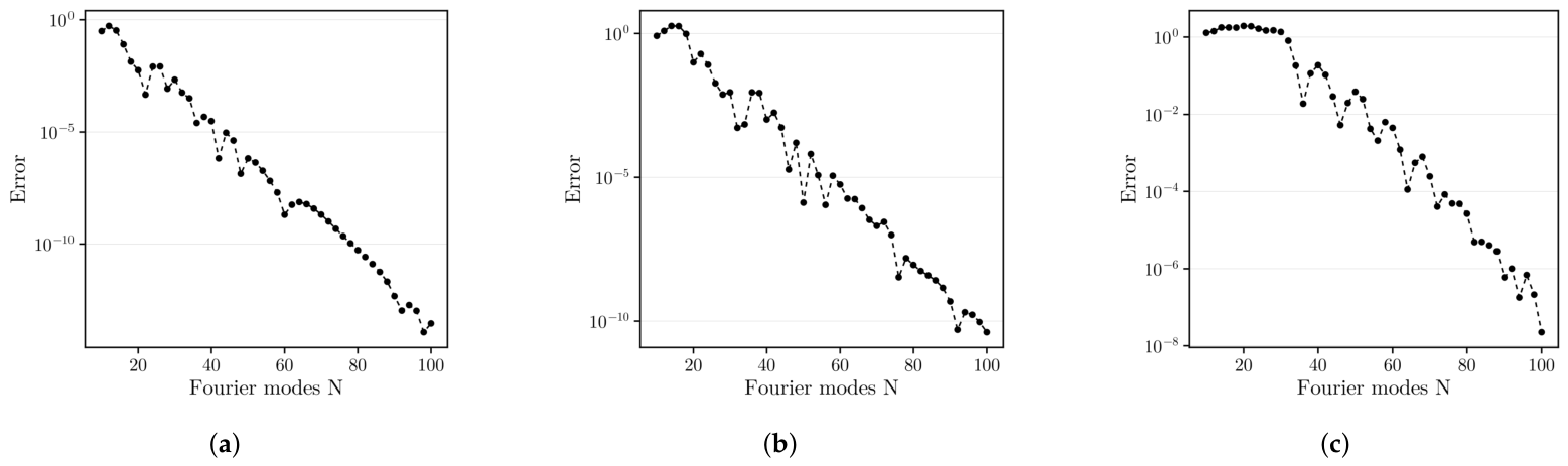
Figure 1 shows the approximation error as a function of the number of Fourier modes for $k=5,10,20$, with $|{\zeta }_0|=0.5$, evaluated at $W_{{\zeta }_0}({\zeta }_0{e}^{-i{\varphi }_t},t)$ with ${\varphi }_t=0.513,0.731,0.970$ and $t=0.0342,0.0231,0.0149$, respectively.

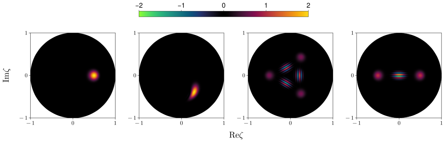
Figure 2 shows the resulting phase-space distribution for several evolution times. The initially localized coherent-state profile first undergoes a squeezing-like deformation. At later times,  nonlinear dynamics lead to the formation of multiple copies of the initial state, with interference fringes appearing in the regions between them; see [34] for a more detailed analysis of this phenomenon.

4.3. Noncompact Evolution: $\widehat{H}={\widehat{K}}_2^2$ (Levin-Type Method)

In the noncompact case, the one-parameter subgroup generated by ${\widehat{K}}_2$ acts as a boost on the Poincaré disk. The integral representation (16) remains valid, but the orbits are not periodic, so the Fourier reduction of the preceding subsection is unavailable, and the oscillatory integrals must be evaluated directly. The evolved state reads

$$|\psi \left(t\right)\rangle ={\displaystyle \frac{1}{\sqrt{i\pi }}}{\int }_{-\infty }^{\infty }dx{e}^{i{x}^2}{e}^{-ik\Phi \left(x\sqrt{t}\right)}|\gamma \left(x\sqrt{t}\right)\rangle ,$$

(22)

where the non-compact group action is parametrized by

$$\xi \left(x\right)=tanh\left(x\right),\gamma \left(x\right)={\displaystyle \frac{\xi \left(x\right)+{\zeta }_0}{1+\xi \left(x\right){\zeta }_0}},\Phi \left(x\right)=2\mathrm{Arg}\left(1+\xi \left(x\right){\zeta }_0\right).$$

(23)

The corresponding Wigner function is

$$W_{{\zeta }_0}(\zeta ,t)={\displaystyle \frac{2}{\pi (2k-1)}}{\int }_{-\infty }^{\infty }{\int }_{-\infty }^{\infty }dxdy{e}^{i(x^2-y^2)}f\left(\xi \left(x\sqrt{t}\right),\xi \left(y\sqrt{t}\right);{\zeta }_0\right)g_k\left(\Lambda (x\sqrt{t},y\sqrt{t};\zeta ,{\zeta }_0)\right),$$

(24)

with the amplitude and auxiliary functions defined by

$$\begin{array}{cc}\hfill f(u,v;{\zeta }_0)& ={(1-u^2)}^k{(1-v^2)}^k{\left(1-uv+{\displaystyle \frac{2i|{\zeta }_0|sin{\phi }_0}{1-|{\zeta }_0{|}^2}}(v-u)\right)}^{-2k},\hfill \end{array}$$

(25)

$$\begin{array}{cc}\hfill \Lambda (x,y;\zeta ,{\zeta }_0)& ={\displaystyle \frac{2\left(1-{\zeta }^{*}\gamma \left(x\right)\right)\left(1-\zeta \overline{\gamma \left(y\right)}\right)}{{(1-|\zeta |}^2)\left(1-\gamma \left(x\right)\overline{\gamma \left(y\right)}\right)}}-1,\hfill \end{array}$$

(26)

$$\begin{array}{cc}\hfill g_k\left(s\right)& ={\int }_0^{\infty }d\mu \mu tanh\left(\pi \mu \right){\Phi }_k^{1/2}\left(\mu \right)P_{-{\displaystyle \frac{1}{2}}+i\mu }\left(s\right),\hfill \end{array}$$

(27)

$$\begin{array}{cc}\hfill {\Phi }_k\left(\mu \right)& ={\displaystyle \frac{(2k-1){\left|\Gamma \left(2k-\frac{1}{2}+i\mu \right)\right|}^2}{{\Gamma }^2\left(2k\right)}},\hfill \end{array}$$

(28)

where in Equation (24) the function $g_k$ is evaluated at $s=\Lambda (x\sqrt{t},y\sqrt{t};\zeta ,{\zeta }_0)$ as defined above, and $P_{\nu }$ denotes the Legendre function of the first kind.

4.3.1. Levin-Type Numerical Evaluation

The rapid oscillations in Equation (24) are handled using a Levin-type method [25,26], which transforms the oscillatory integral into the solution of auxiliary differential equations. Starting from the generic two-dimensional oscillatory integral (mapped to the unit domain by an appropriate change in variables)

$$I={\int }_{-1}^1{\int }_{-1}^{1}dxdyf(x,y)e^{ig(x,y)},$$

(29)

we treat the integral in an iterated manner. For the inner integral in y, we introduce an auxiliary function $p(x,y)$ satisfying

$${\displaystyle \frac{\partial p}{\partial y}}+i{\displaystyle \frac{\partial g}{\partial y}}p=f(x,y),$$

(30)

so that

$$I\left(x\right)={\int }_{-1}^{1}dyf(x,y)e^{ig(x,y)}=p(x,1)e^{ig(x,1)}-p(x,-1)e^{ig(x,-1)}.$$

(31)

The differential Equation (30) is discretized using Chebyshev–Lobatto nodes

$$x_j=cos\left({\displaystyle \frac{j\pi }{N}}\right),y_m=cos\left({\displaystyle \frac{m\pi }{N}}\right),j,m=0,\dots ,N,$$

(32)

together with the Chebyshev differentiation matrix [35] ${\mathit{D}}^{\left(N\right)}\in {\mathbb{R}}^{(N+1)\times (N+1)}$ with entries

$$D_{ij}=\left\{\begin{array}{cc}{\displaystyle \frac{c_i}{c_j}}{\displaystyle \frac{{(-1)}^{i+j}}{x_i-x_j}},\hfill & i\ne j,\hfill \\ {\displaystyle -\sum _{\begin{array}{c}\ell =0\\ \ell \ne i\end{array}}^N{D}_{i\ell },}\hfill & i=j,\hfill \end{array}\right.c_0=c_N=2,c_j=1(1\le j\le N-1).$$

(33)

If $\mathit{f}={(f\left(x_0\right),\dots ,f\left(x_N\right))}^{\top }$ denotes the vector composed of the function values of f at the Chebyshev–Lobatto nodes, then ${\mathit{f}}^{\prime }={(f^{\prime }\left(x_0\right),\dots ,f^{\prime }\left(x_N\right))}^{\top }$ is given by the matrix product

$${\mathit{f}}^{\prime }=\mathit{D}\mathit{f}.$$

(34)

Then, for each fixed $x_j$, Equation (30) leads to the linear system

$$\left(\mathit{D}+i{\mathit{G}}_j\right){\mathit{p}}_j={\mathit{f}}_j,j=0,\dots ,N,$$

(35)

where

$${\mathit{p}}_j={\left(p(x_j,y_0),\dots ,p(x_j,y_N)\right)}^{\top },{\mathit{f}}_j={\left(f(x_j,y_0),\dots ,f(x_j,y_N)\right)}^{\top },$$

(36)

and ${\mathit{G}}_j$ is a diagonal matrix with entries ${\left({\mathit{G}}_j\right)}_{mm}={\partial }_{y}g(x_j,y_m)$.

Solving these $N+1$ systems yields the values of $p(x_j,y_m)$ at the full set of collocation nodes.

The outer integral is treated analogously by introducing auxiliary functions $q_{\pm }\left(x\right)$ satisfying

$${\displaystyle \frac{d{q}_{\pm }}{dx}}+i{\displaystyle \frac{\partial g}{\partial x}}(x,\pm 1)q_{\pm }=p(x,\pm 1),$$

(37)

which lead to

$$I=q_{+}\left(1\right)e^{ig(1,1)}-q_{+}(-1)e^{ig(-1,1)}-q_{-}\left(1\right)e^{ig(1,-1)}+q_{-}(-1)e^{ig(-1,-1)}.$$

(38)

Discretization in x yields the linear systems

$$(\mathit{D}+i{\mathit{G}}_{\pm }){\mathit{q}}_{\pm }={\mathit{p}}_{\pm },$$

(39)

where ${\left({\mathit{G}}_{\pm }\right)}_{mm}={\partial }_{x}g(x_m,\pm 1)$ and ${\mathit{p}}_{\pm }={\left(p(x_0,\pm 1),\dots ,p(x_N,\pm 1)\right)}^{\top }$.

Domain Truncation

Since the integration domain in Equation (24) is the entire plane, the Levin scheme is applied on a finite domain containing the effective support of the integrand. This is justified by the rapid suppression of the integrand away from the origin due to the combined effect of growing oscillations in the phase and the decay in the amplitude. Rescaling the integration variable makes the role of t explicit:

$$\begin{array}{cc}\hfill W_{{\zeta }_0}(\zeta ,t)={\displaystyle \frac{2}{t\pi (2k-1)}}{\int }_{-\infty }^{\infty }{\int }_{-\infty }^{\infty }dxdy& e^{i(x^2-y^2)/t}f\left(\xi \left(x\right),\xi \left(y\right);{\zeta }_0\right)\hfill \\ \hfill & \times g_k\left(\Lambda (x,y;\zeta ,{\zeta }_0)\right).\hfill \end{array}$$

(40)

In the short-time regime ($t\ll 1$), the factor $1/t$ in the oscillatory phase confines the dominant contribution to a small neighborhood of the origin via destructive interference (stationary-phase suppression). At later times, the effective support is instead governed by the amplitude decay of f and $g_k$. The integration domain therefore undergoes a crossover from a phase-controlled regime to an amplitude-controlled regime as t increases.

Because Chebyshev nodes cluster near the interval endpoints, the accuracy near the unique stationary point at the origin is enhanced by partitioning the domain into four quadrants so that the critical point lies at a corner of each subdomain, as recommended in [25].

Adaptive Refinement

The number of collocation nodes is increased progressively until a difference-based error estimator falls below a prescribed tolerance $\epsilon$. The procedure is summarized in Algorithm 1, where $I_N$ denotes the numerical approximation obtained using N Chebyshev nodes per dimension.

Algorithm 1 Adaptive Levin refinement.

1: Set initial resolution N; compute $I_0\leftarrow I_N$. 2: Compute refinement $I_{2N}$. 3: if  $|I_{2N}-I_0|<\epsilon max(1,|I_{2N}\left|\right)$  then 4:       Accept $I_{2N}$. 5: else 6:       Set $I_0\leftarrow I_{2N}$, $N\leftarrow 2N$; repeat from Step 2. 7: end if

Since Chebyshev–Lobatto nodes are nested ($\left\{x_j^{\left(N\right)}\right\}\subset \left\{x_j^{\left(2N\right)}\right\}$ with $x_j^{\left(N\right)}=x_{2j}^{\left(2N\right)}$), the previously computed function evaluations are reused at each refinement step, reducing the overall computational cost.

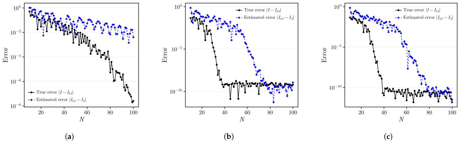
Figure 3 compares the true error $|I-I_{2N}|$ with the estimator $|I_{2N}-I_N|$ in the computation of $W_{{\zeta }_0}(0,t)$ for ${\zeta }_0=0$. The estimator overestimates the true error across the tested regime, indicating its conservative character and suitability for adaptive control.

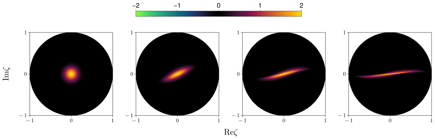
Figure 4 shows the resulting phase-space distribution for several evolution times. The initially localized coherent-state profile becomes progressively distorted as the nonlinear dynamics generate a squeezing-type deformation.

5. Conclusions

We analyzed the phase-space dynamics of $\mathrm{SU}(1,1)$ systems by combining geometric analysis, pseudodifferential operator theory, and numerical computation. The evolution equation naturally couples transport dynamics with the spectral functions of the Casimir operator, which act as pseudodifferential operators on the hyperbolic disk. The pseudodifferential structure yields a concrete PDE classification: the compact generator ${\widehat{K}}_0$ produces a degenerate hyperbolic operator of transport type, while the noncompact generator ${\widehat{K}}_2$ produces a mixed-order differential–pseudodifferential operator. In the compact case, periodicity of the group orbits enables a Fourier reduction with analytic time dependence; in the noncompact case, the resulting oscillatory integrals are handled efficiently by a Levin-type spectral collocation method. Both strategies are free of the stiffness and spurious oscillation issues that afflict direct PDE evolution near the noncompact boundary, and they produce phase-space dynamics consistent with the underlying unitary evolution.

Natural extensions of this framework include the treatment of more general quadratic combinations of the generators, the analysis of analogous systems with $\mathrm{SU}\left(2\right)$ symmetry on the compact phase space, and the application of the Levin-type method to initial states beyond the coherent class.

References

- Ou, Z.Y. Quantum SU(1,1) interferometers: Basic principles and applications. APL Photonics 2020, 5, 080902. [Google Scholar] [CrossRef]
- Metzner, J.; Quinn, A.; Brudney, S.; Moore, I.D.; Burd, S.C.; Wineland, D.J.; Allcock, D.T.C. Two-mode squeezing and SU(1,1) interferometry with trapped ions. arXiv 2023, arXiv:2312.10847. [Google Scholar] [CrossRef]
- Hudelist, F.; Kong, J.; Liu, C.; Jing, J.; Ou, Z.; Zhang, W. Quantum metrology with parametric amplifier-based photon correlation interferometers. Nat. Commun. 2014, 5, 3049. [Google Scholar] [CrossRef]
- Ojeda-Guillén, D.; Mota, R.D.; Granados, V.D. The SU(1,1) Perelomov number coherent states and the non-degenerate parametric amplifier. arXiv 2013, arXiv:1311.6867. [Google Scholar] [CrossRef]
- Teich, M.C.; Saleh, B.E.A. Squeezed states of light. Quantum Opt. 1990, 1, 153–191. [Google Scholar] [CrossRef]
- Shaterzadeh-Yazdi, Z.; Turner, P.S.; Sanders, B.C. SU(1,1) symmetry of multimode squeezed states. arXiv 2007, arXiv:0710.3205. [Google Scholar] [CrossRef]
- Zachos, C.; Fairlie, D.; Curtright, T. Quantum Mechanics in Phase Space: An Overview with Selected Papers; World Scientific: Singapore, 2005. [Google Scholar]
- Brif, C.; Mann, A. Phase-space formulation of quantum mechanics and quantum-state reconstruction for physical systems with Lie-group symmetries. Phys. Rev. A 1999, 59, 971–987. [Google Scholar] [CrossRef]
- Perelomov, A.M. Generalized Coherent States and Their Applications; Texts and Monographs in Physics; Springer: Berlin/Heidelberg, Germany, 1986. [Google Scholar] [CrossRef]
- Shao, S.; Lu, T.; Cai, W. Adaptive conservative cell average spectral element methods for transient Wigner equation in quantum transport. Commun. Comput. Phys. 2011, 9, 711–739. [Google Scholar] [CrossRef]
- Shao, S.; Sellier, J.M. Comparison of deterministic and stochastic methods for time-dependent Wigner simulations. J. Comput. Phys. 2015, 300, 167–185. [Google Scholar] [CrossRef]
- Cabrera, R.; Bondar, D.I.; Jacobs, K.; Rabitz, H.A. Efficient method to generate time evolution of the Wigner function for open quantum systems. Phys. Rev. A 2015, 92, 042122. [Google Scholar] [CrossRef]
- Xiong, Y.; Chen, Z.; Shao, S. An advective-spectral-mixed method for time-dependent many-body Wigner simulations. SIAM J. Sci. Comput. 2016, 38, B491–B520. [Google Scholar] [CrossRef]
- Klimov, A.B. Exact evolution equations for SU (2) quasidistribution functions. J. Math. Phys. 2002, 43, 2202–2213. [Google Scholar] [CrossRef]
- Kalmykov, Y.P.; Coffey, W.T.; Titov, S.V. Phase-space formulation of the nonlinear longitudinal relaxation of the magnetization in quantum spin systems. Phys. Rev. E 2007, 76, 051104. [Google Scholar] [CrossRef]
- Benkaddour, A.; Ouari, B. Unified quantum-classical description of spin dynamics via the Wigner–Stratonovich transformation. Appl. Phys. A 2026, 132, 259. [Google Scholar] [CrossRef]
- Klimov, A.B.; Seyfarth, U.; de Guise, H.; Sánchez-Soto, L.L. SU(1,1) covariant s-parametrized maps. J. Phys. A Math. Theor. 2021, 54, 065301. [Google Scholar] [CrossRef]
- Akhtar, N.; Sanders, B.C.; Xianlong, G. Sub-Planck phase-space structure and sensitivity for SU (1,1) compass states. Phys. Rev. A 2022, 106, 043704. [Google Scholar] [CrossRef]
- Baltazar, M.; Valtierra, I.F.; Klimov, A.B. Correspondence Rules for SU(1,1) Quasidistribution Functions and Quantum Dynamics in the Hyperbolic Phase Space. Entropy 2022, 24, 1580. [Google Scholar] [CrossRef]
- Baltazar, M.; Valtierra, I.F.; Klimov, A.B. Quantum systems in the hyperbolic phase-space: Explicit maps, differential form of the star product and their applications. Ann. Phys. 2025, 482, 170208. [Google Scholar] [CrossRef]
- Khorasani, S. Solution of cross-Kerr interaction combined with parametric amplification. Sci. Rep. 2019, 9, 1830. [Google Scholar] [CrossRef] [PubMed]
- Semião, F.L.; Vidiella-Barranco, A. Effective cross-Kerr nonlinearity and robust phase gates with trapped ions. Phys. Rev. A 2005, 72, 064305. [Google Scholar] [CrossRef]
- Zou, F.; Fan, L.B.; Huang, J.F.; Liao, J.Q. Enhancement of few-photon optomechanical effects with cross-Kerr nonlinearity. Phys. Rev. A 2019, 99, 043837. [Google Scholar] [CrossRef]
- Valtierra, I.F.; Klimov, A.B. Tunneling currents in the hyperbolic phase space. Entropy 2024, 26, 639. [Google Scholar] [CrossRef]
- Li, J.; Wang, X.; Wang, T.; Shen, C. Delaminating quadrature method for multi-dimensional highly oscillatory integrals. Appl. Math. Comput. 2009, 209, 327–338. [Google Scholar] [CrossRef]
- Li, J.; Wang, X.; Wang, T.; Xiao, S. An improved Levin quadrature method for highly oscillatory integrals. Appl. Numer. Math. 2010, 60, 833–842. [Google Scholar] [CrossRef]
- Bargmann, V. Irreducible unitary representations of the Lorentz group. Ann. Math. 1947, 48, 568–640. [Google Scholar] [CrossRef]
- Zhang, W.M.; Gilmore, R.; Feng, D.H. Coherent states: Theory and some applications. Rev. Mod. Phys. 1990, 62, 867. [Google Scholar] [CrossRef]
- Lindblad, G.; Nagel, B. Continuous bases for unitary irreducible representations of SU (1,1). Ann. Inst. H. Poincaré Sect. A 1970, 13, 27–56. [Google Scholar]
- Helgason, S. Groups and Geometric Analysis: Integral Geometry, Invariant Differential Operators, and Spherical Functions; Academic Press: Orlando, FL, USA, 1984. [Google Scholar]
- Wallach, N.R. Real Reductive Groups I; Academic Press: San Diego, CA, USA, 1988; Volume 132. [Google Scholar]
- Helgason, S. Geometric Analysis on Symmetric Spaces. In Mathematical Surveys and Monographs; American Mathematical Society: Providence, RI, USA, 2008; Volume 39. [Google Scholar] [CrossRef]
- Perelomov, A.M. Generalized coherent states and some of their applications. Sov. Phys. Uspekhi 1977, 20, 703–720. [Google Scholar] [CrossRef]
- Banerji, J.; Agarwal, G.S. Revival and fractional revival in the quantum dynamics of SU (1,1) coherent states. Phys. Rev. A 1999, 59, 4777. [Google Scholar] [CrossRef]
- Canuto, C.; Hussaini, M.Y.; Quarteroni, A.; Zang, T.A. Spectral Methods. In Scientific Computation Ser.; Springer: Berlin/Heidelberg, Germany, 2006; Volume 285, pp. e1–e4. [Google Scholar] [CrossRef]
- Varadarajan, V.S. Lie Groups, Lie Algebras, and Their Representations; Springer: New York, NY, USA, 1984. [Google Scholar]
- Hörmander, L. The Analysis of Linear Partial Differential Operators III: Pseudo-Differential Operators; Springer Science & Business Media: Berlin/Heidelberg, Germany, 2007. [Google Scholar]
- Taylor, M.E. Partial Differential Equations III; Springer: Berlin/Heidelberg, Germany, 1996; Volume 2. [Google Scholar]
- Shubin, M.A. Pseudodifferential Operators and Spectral Theory; Springer: Berlin/Heidelberg, Germany, 1987; Volume 57. [Google Scholar]