Hierarchical Multi-View Representation Learning via Generalized Deep Non-Negative Matrix Factorization

Abstract

Multi-view clustering aims to exploit complementary information from multiple views to uncover intrinsic grouping structures in data, where effective representation learning plays a critical role. Non-negative matrix factorization (NMF) has been widely used for multi-view representation learning due to its inherent interpretability; however, most existing NMF-based methods rely on shallow architectures and are therefore insufficient for capturing hierarchical characteristics. Although recent deep NMF models introduce multi-layer structures by factorizing either feature matrices or basis matrices, their performance may degrade when the data are limited or exhibit relatively simple structures. To address these issues, this paper proposes a generalized deep non-negative matrix factorization framework for multi-view representation learning, termed GDNMF-MRL, which jointly decomposes feature and basis matrices to learn hierarchical representations. By integrating shallow linear components with deep nonlinear structures, the proposed method enhances representation capability and yields more discriminative latent subspaces. Furthermore, a one-step variant, termed OS-GDNMF-MRL, is developed to simultaneously learn latent representations and clustering assignments within a unified optimization framework, enabling direct interaction between representation learning and clustering without requiring separate post-processing. Two efficient alternating optimization algorithms with guaranteed convergence of the objective function are derived, and extensive experiments on benchmark datasets demonstrate that the proposed methods consistently outperform several state-of-the-art multi-view clustering approaches.

1. Introduction

In recent years, increasing amounts of data have been generated from multiple views. For example, images can be described by different feature types, such as color, texture, and edge information; videos naturally contain both visual and audio components; and textual content may be represented in multiple languages [1,2]. In addition, the same object may have different representations owing to different data acquisition processes. Such data are generally referred to as multi-view data, in which each view captures useful characteristics of the underlying object while also introducing its own bias. Multi-view data arise naturally and frequently in practical applications, giving rise to a new learning paradigm known as multi-view representation learning (MRL) [3]. MRL aims to learn informative representations (or features) from multi-view data to support downstream predictive tasks. When these learned representations are used for clustering, the resulting problem is referred to as multi-view clustering (MVC), which exploits information from multiple views, leverages the strengths of each view, and mitigates their individual limitations to achieve accurate and robust clustering performance. This paradigm has attracted increasing attention in unsupervised learning and has been applied in many practical domains, including computer vision (CV) [4], natural language processing (NLP), social multimedia, bioinformatics, and health informatics [5]. In CV, MVC techniques have been widely used for image classification, motion segmentation, and group detection. In NLP, text documents can be represented in multiple languages, where each language serves as a distinct view, making MVC naturally applicable to document analysis tasks.

A variety of multi-view clustering methods have been proposed, leading to notable progress in this research area. An intuitive solution for multi-view representation learning is to directly concatenate features from all views and apply conventional single-view learning techniques [6]. However, this straightforward strategy often suffers from overfitting on small-scale datasets and fails to preserve the distinct statistical properties inherent to each view. To overcome these limitations, numerous approaches have been explored in recent years, including kernel-based techniques [7,8], subspace clustering methods [9,10], and spectral learning approaches [11], as well as representation learning frameworks based on autoencoders and matrix factorization [12,13], which aim to more effectively integrate complementary information across multiple views.

Non-negative matrix factorization (NMF) [14] factorizes each view into low-dimensional basis and coefficient matrices under non-negativity constraints, resulting in additive and interpretable representations. This property makes NMF well suited for real-world scenarios in which negative values lack physical meaning, such as image intensities, word frequencies, and gene expression data. To relax the strict non-negativity requirement, semi-NMF [15] removes the constraint on the basis matrix and the data matrix, thereby extending the applicability of NMF to more general data distributions. From a clustering perspective, semi-NMF can be interpreted such that the basis matrix represents cluster centroids, while the coefficient matrix encodes cluster assignments. Beyond unsupervised settings, semi-supervised NMF methods incorporate prior label information to guide representation learning and can be broadly divided into hard-constraint and soft-constraint approaches [16]. Hard-constraint methods [17,18] enforce identical representations for samples sharing the same labels, whereas soft-constraint methods [19,20] introduce regularization terms to encourage similarity while allowing flexibility among labeled samples. Owing to its ability to project high-dimensional data into compact non-negative spaces, NMF and its variants are particularly advantageous for multi-view clustering, where they preserve global structures while retaining view-specific characteristics, and have therefore attracted considerable attention in multi-view clustering research.

Conventional single-layer non-negative matrix factorization primarily captures shallow representations and is therefore insufficient for modeling the complex hierarchical structures commonly observed in real-world data. To address this limitation, deep NMF models with multi-layer architectures have been introduced, in which hierarchical representations are constructed by recursively factorizing either the feature matrix or the basis matrix into multiple components [21,22]. Through such layered decomposition, deep NMF can uncover latent hierarchical features and generate multi-level representations, leading to improved performance in representation learning and clustering. However, existing approaches still suffer from several critical limitations. First, most deep NMF methods are restricted to a single decomposition direction; that is, they can perform deep factorization on either the feature matrix or the basis matrix, but cannot jointly model hierarchical structures in both spaces within a unified framework. Second, current multi-view NMF methods mainly rely on shallow matrix factorization and therefore cannot effectively integrate deep hierarchical representation learning with cross-view information fusion. Third, most multi-view clustering frameworks decouple representation learning from clustering assignment, preventing clustering information from directly guiding representation learning during optimization.

To address the above limitations, this paper proposes GDNMF-MRL, a generalized deep non-negative matrix factorization framework for multi-view representation learning. In contrast to previous deep NMF or multi-view NMF methods, GDNMF-MRL jointly decomposes basis matrices and feature matrices for each view and combines a deep nonlinear reconstruction term with a shallow linear term, so that both hierarchical structure and simple linear information can be preserved within one multi-view model. On top of this framework, we further introduce OS-GDNMF-MRL. Importantly, OS-GDNMF-MRL is not a post-processing integration of k-means applied after representation learning; instead, it embeds the clustering label matrix directly into the objective function and jointly updates representation variables and clustering assignments during optimization. The main contributions of this work are summarized as follows:

• We propose GDNMF-MRL, a unified framework that simultaneously performs deep decomposition on both feature matrices and basis matrices, enabling hierarchical representations to be extracted at multiple levels. By integrating shallow linear components and deep nonlinear structures in a complementary manner, the proposed framework preserves both simple linear information and complex hierarchical patterns, improving the flexibility and discriminative power of the learned representations.
• We design a multi-view fusion mechanism that learns adaptive view weights while enforcing cross-view consistency through a shared consensus representation, allowing the model to effectively exploit complementary information across heterogeneous views.
• We further develop a one-step variant, OS-GDNMF-MRL, which jointly optimizes representation learning and clustering assignment within a unified objective function, enabling direct interaction between the two stages and avoiding the suboptimality of conventional two-step procedures.
• Extensive experiments on five benchmark datasets demonstrate that the proposed methods consistently outperform state-of-the-art shallow and deep multi-view clustering approaches, validating the effectiveness and robustness of the proposed framework.

The remainder of this paper is organized as follows. Section 2 reviews the foundations of single-view GDNMF and related multi-view representation learning methods. Section 3 introduces the proposed GDNMF-MRL and OS-GDNMF-MRL frameworks. Section 4 presents the corresponding optimization algorithms and computational complexity analysis. Experimental results and performance comparisons are presented in Section 5, followed by concluding remarks in Section 6.

2. Related Works

In this section, we first revisit the single-view generalized deep NMF model and then review the MRL methods most closely related to our work.

2.1. Single-View GDNMF

The original data are represented as $\mathbf{X}=[{\mathbf{x}}_1,{\mathbf{x}}_2,\cdots ,{\mathbf{x}}_n]\in {\mathbb{R}}^{p\times n}$, where each column represents a sample described by p features. Deep Semi-NMF (DSNMF) [21] extends shallow NMF by introducing a multi-layer factorization of the feature matrix, which can be written as

$$\widehat{\mathbf{X}}={\mathbf{W}}_1{\mathbf{W}}_2\cdots {\mathbf{W}}_m{\mathbf{H}}_m,$$

(1)

where the intermediate representations satisfy ${\mathbf{H}}_i={\mathbf{W}}_{i+1}{\mathbf{H}}_{i+1}$ for $i=1,2,\cdots$, $m-1$. Here, ${\mathbf{W}}_i$ and ${\mathbf{H}}_i$ denote the basis and feature matrices at the i-th layer, respectively. Although DSNMF is able to learn more expressive low-dimensional representations than shallow NMF, only the first-layer basis matrix ${\mathbf{W}}_1$ is directly related to the original data, which limits its ability to simultaneously model high-level and local bases. Nonlinear DSNMF further introduces nonlinear activation functions between successive layers to approximate nonlinear manifolds, but the above limitation still remains.

Different from deep feature decomposition, deep non-negative basis matrix factorization (DNBMF) [22] performs hierarchical decomposition on the basis matrix and represents the data as

$$\widehat{\mathbf{X}}={\mathbf{W}}_m{\mathbf{H}}_m\cdots {\mathbf{H}}_2{\mathbf{H}}_1,$$

(2)

with ${\mathbf{W}}_i={\mathbf{W}}_{i+1}{\mathbf{H}}_{i+1}$, $i=1,2,\cdots$, $m-1$. This strategy enables the extraction of deep local basis structures; however, since only the first-layer feature matrix ${\mathbf{H}}_1$ is directly associated with $\mathbf{X}$, hierarchical feature representations are not explicitly preserved.

To overcome these limitations, generalized deep non-negative matrix factorization (GDNMF) [23] simultaneously considers both feature and basis hierarchies. In the first layer, the data matrix $\mathbf{X}\in {\mathbb{R}}^{p\times n}$ is decomposed as

$$\begin{array}{cc}\hfill & \widehat{\mathbf{X}}={\mathbf{F}}_1{\mathbf{S}}_1{\mathbf{G}}_1,\hfill \\ \hfill \mathrm{s}.\mathrm{t}.& {\mathbf{F}}_1\ge 0,{\mathbf{S}}_1\ge 0,{\mathbf{G}}_1\ge 0,\hfill \end{array}$$

(3)

where ${\mathbf{F}}_1$ and ${\mathbf{G}}_1$ denote the basis and feature matrices, respectively, and ${\mathbf{S}}_1$ is an auxiliary matrix modeling their interactions.

For basis decomposition, ${\mathbf{F}}_1$ is recursively factorized according to ${\mathbf{F}}_i\approx {\mathbf{F}}_{i+1}{\mathbf{L}}_{i+1}$, leading to

$$\begin{array}{cc}\hfill & {\widehat{\mathbf{F}}}_1={\mathbf{F}}_{m_1}{\mathbf{L}}_{m_1}{\mathbf{L}}_{m_1-1}\cdots {\mathbf{L}}_2,\hfill \\ \hfill \mathrm{s}.\mathrm{t}.& {\mathbf{F}}_i\ge 0,{\mathbf{L}}_i\ge 0,i=1,2,\cdots ,m_1,\hfill \end{array}$$

(4)

where $m_1$ denotes the number of layers for basis decomposition.

Similarly, feature decomposition is performed by recursively factorizing ${\mathbf{G}}_1$ as ${\mathbf{G}}_i\approx {\mathbf{R}}_{i+1}{\mathbf{G}}_{i+1}$, which yields

$$\begin{array}{cc}\hfill & {\widehat{\mathbf{G}}}_1={\mathbf{R}}_2{\mathbf{R}}_3\cdots {\mathbf{R}}_{m_2}{\mathbf{G}}_{m_2},\hfill \\ \hfill \mathrm{s}.\mathrm{t}.& {\mathbf{G}}_i\ge 0,{\mathbf{R}}_i\ge 0,i=1,2,\cdots ,m_2,\hfill \end{array}$$

(5)

where $m_2$ is the depth of feature decomposition.

To capture nonlinear hierarchical relationships in real-world data, nonlinear activation functions $g(·)$ are introduced between successive layers: ${\widehat{\mathbf{F}}}_i=g\left({\mathbf{F}}_{i+1}{\mathbf{L}}_{i+1}\right)$ and ${\widehat{\mathbf{G}}}_i=g\left({\mathbf{R}}_{i+1}{\mathbf{G}}_{i+1}\right)$. However, when data are limited or exhibit relatively simple structures, purely deep nonlinear models may increase computational complexity without clear benefits. To alleviate this issue, shallow linear components are incorporated into the deep framework, enabling complementary modeling of both linear and nonlinear information. Consequently, the final optimization problem is formulated as

$$\begin{array}{cc}\hfill \underset{\mathbf{F},\mathbf{S},\mathbf{G},\mathbf{W}\ge 0}{\min }& {\displaystyle \frac{1}{2}}{\parallel \mathbf{X}-{\widehat{\mathbf{F}}}_1{\mathbf{S}}_1{\widehat{\mathbf{G}}}_1-\mathbf{W}{\mathbf{G}}_{m_2}\parallel }_F^2\hfill \\ \hfill \mathrm{s}.\mathrm{t}.& {\widehat{\mathbf{F}}}_1=g\left(g\left({\mathbf{F}}_{m_1}{\mathbf{L}}_{m_1}\right){\mathbf{L}}_{m_1-1}\cdots {\mathbf{L}}_2\right),\hfill \\ \hfill & {\widehat{\mathbf{G}}}_1=g\left({\mathbf{R}}_{2}g(\cdots {\mathbf{R}}_{m_2-1}g\left({\mathbf{R}}_{m_2}{\mathbf{G}}_{m_2}\right))\right).\hfill \end{array}$$

(6)

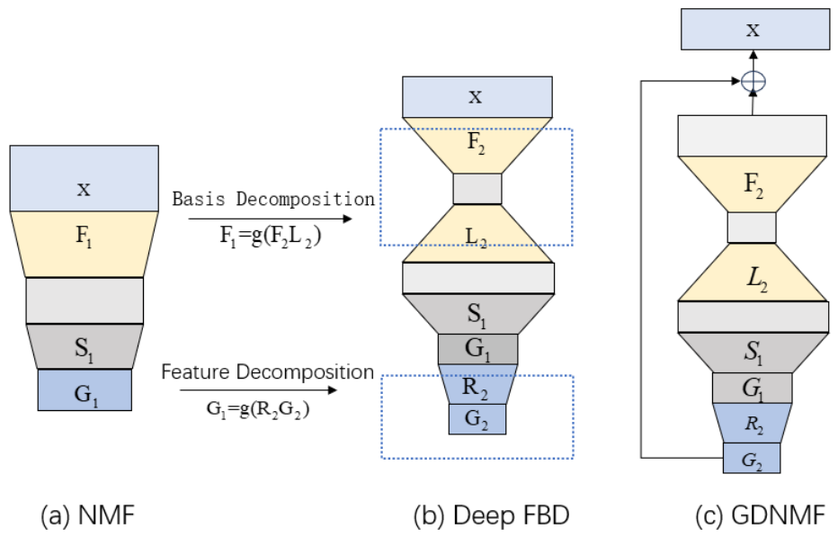
As shown in Figure 1, GDNMF uses the summation of deep nonlinear ${\widehat{\mathbf{F}}}_1{\mathbf{S}}_1{\widehat{\mathbf{G}}}_1$ and shallow linear $\mathbf{W}{\mathbf{G}}_2$ to reconstruct $\mathbf{X}$. However, advanced deep decomposition methods based on NMF have failed to address MRL problems.

2.2. Related Work

In recent years, a wide range of multi-view representation learning (MRL) methods have been developed to address the challenges posed by multi-view data analysis. Early attempts often extended classical learning techniques to the multi-view setting. Among them, k-nearest neighbor (KNN)-based methods have been successfully applied to graph learning [24], spectral learning, and multi-view learning tasks [25,26]. To alleviate the sensitivity of KNN to the choice of neighborhood size, Zhang et al. [27] proposed an adaptive KNN model that automatically learns optimal k values for different samples. Building upon this idea, Jiang et al. [28] further integrated adaptive KNN with multi-view spectral learning in a unified framework to better exploit heterogeneous information across views.

Canonical correlation analysis (CCA)-based approaches constitute another important branch of MRL. These methods aim to learn correlated representations across multiple views. Andrew et al. [29] extended classical CCA to deep CCA by learning nonlinear transformations for two views, enabling more expressive cross-view correlations. However, CCA-based methods are inherently limited to two-view scenarios and thus lack flexibility for general multi-view data.

Multi-view subspace clustering methods attempt to represent data segmentation in a shared low-dimensional space by learning low-rank representations [30,31]. To uncover common structures shared across views, Zhang et al. [32] introduced latent multi-view subspace clustering. By leveraging tensor learning, Xiao et al. [33] proposed a prior-knowledge-regularized multi-view self-representation model that captures high-order correlations and incorporates label information. Several spectral-based multi-view clustering models have also been proposed, including unified one-step spectral clustering [34] and graph-based multi-view clustering with automatic fusion strategies [35]. Despite their effectiveness, spectral methods usually suffer from high computational complexity, which limits their applicability to large-scale datasets.

Deep learning-based MRL methods have recently attracted increasing attention due to their powerful nonlinear modeling capabilities. Wang et al. [36] combined deep CCA with autoencoders to develop a deep canonical correlation autoencoder (DCCAE). Xu et al. [37] proposed a generative multi-view clustering framework based on variational autoencoders (multi-VAE) to learn disentangled representations. Zhang et al. [38] introduced an unsupervised framework with internal and external autoencoder networks, while Yang et al. [39] designed a unified autoencoder-based model to handle partial view misalignment and missing samples. Nevertheless, most deep autoencoder-based approaches neglect the non-negativity constraint of data, which reduces interpretability, and they generally lack theoretical convergence guarantees in unsupervised settings.

Non-negative matrix factorization (NMF) has been widely recognized as an effective tool for dimensionality reduction and representation learning due to its interpretability and ability to reveal latent data structures [14,40]. In the multi-view setting, Liu et al. [41] constructed view-specific coefficient matrices and encouraged them to converge to a consensus representation. Orthogonality constraints, which have shown strong performance in single-view NMF, were extended to multi-view scenarios by Wang et al. [42] through diversity-induced NMF (DiNMF). Liang et al. [43] further proposed co-orthogonal constraints on both basis and representation matrices, while Cao et al. [44] developed a diversity-induced multi-view subspace clustering method to exploit complementary information across views.

A representative line of work assumes that different views are intrinsically connected and seeks to maximize their consistency by learning a shared latent representation. MultiNMF is a seminal method in this category, which pulls view-specific low-rank representations toward a single consensus matrix. Following this idea, various extensions have been proposed, including manifold-regularized multi-view NMF [45], multi-manifold NMF [46], and three-factorization-based NMF for uniform distribution modeling [47]. Recent advances further incorporate hypergraph learning [48], unconstrained formulations [49], adaptive graph structures [50], and similarity-induced weighted consensus learning [51]. Semi-supervised and deep matrix factorization variants have also been explored, such as partial shared deep matrix factorization [52], diverse deep matrix factorization with hypergraph regularization [53], and exclusivity–consistency-induced NMF frameworks [54].

Despite their success, existing NMF-based MRL methods still suffer from several limitations. Most single-layer models only capture shallow data structures and fail to model complex hierarchical information. Although deep matrix factorization methods improve representation capacity, they typically focus on either deep feature decomposition or deep basis decomposition, making it difficult to simultaneously model high-level and local bases. Moreover, representation learning and clustering are often treated as two independent stages, preventing learned representations from being refined by clustering feedback. To address these challenges, we propose a generalized deep non-negative matrix factorization framework that integrates hierarchical representation learning and multi-view fusion, and further develop a one-step variant that jointly learns representations and clustering labels. By tightly coupling representation learning with clustering partition fusion, the proposed method avoids additional clustering steps and achieves improved clustering performance. To further clarify the structural differences among representative methods used in the experiments,

Table 1. Structural comparison of representative methods used in the experiments.

Method	Deep Structure	MVC Method	Basis Decomposition	Feature Decomposition	Clustering Integration	Interpretability
NMF						High
MultiNMF		✔				High
ECNMF		✔				High
2CMV		✔				Moderate
DMF	✔			✔		Moderate
DA2NMF	✔	✔		✔		Moderate
DMVC	✔	✔		✔		Moderate
GDNMF	✔		✔	✔		High
MDRNMF	✔	✔	✔	✔		Moderate
GDNMF-MRL	✔	✔	✔	✔		High
OS-GDNMF-MRL	✔	✔	✔	✔	✔	High

summarizes their characteristics in terms of deep structure, decomposition strategy, clustering integration, and interpretability.

Here, “Basis Decomposition” and “Feature Decomposition” denote explicit hierarchical decomposition on the basis side and feature side, respectively. “Clustering Integration” indicates that clustering assignments are optimized directly within the model objective rather than obtained via a separate post-processing step. “Interpretability” is qualitatively evaluated as High, Moderate, or Low according to the extent to which the learned representations preserve part-based semantics, hierarchical structure, and explicit matrix-factorization forms, thereby admitting clear semantic or physical interpretation.

3. Proposed Method

Table 2. Main notations used in Section 3 and Section 4.

Symbol	Description
V	Number of views.
$m_1,m_2$	Numbers of basis-side and feature-side decomposition layers, respectively.
n	Number of samples.
K	Number of clusters.
$\gamma$	Hyperparameter controlling the distribution of adaptive view weights.
$\lambda$	Graph regularization parameter.
${\alpha }^v$	Adaptive weight associated with the v-th view.
${\mathbf{X}}^v$	Data matrix of the v-th view.
${\mathbf{W}}^v$	Linear basis matrix for the shallow component in the v-th view.
${\mathbf{F}}_{m_1}^v$	Top-layer basis matrix in the basis-side deep decomposition of the v-th view.
${\widehat{\mathbf{F}}}_1^v$	Reconstructed basis matrix obtained from the basis-side deep decomposition of the v-th view.
${\mathbf{S}}_1^v$	Interaction matrix linking the reconstructed basis and feature representations in the v-th view.
${\mathbf{G}}_{m_2}^v$	Final latent representation learned from the v-th view.
${\widehat{\mathbf{G}}}_1^v$	Reconstructed feature matrix obtained from the feature-side deep decomposition of the v-th view.
${\mathbf{G}}^{*}$	Consensus latent representation shared by all views.
${\mathbf{L}}_i^v$	Transformation matrix in the i-th layer of basis-side decomposition for the v-th view.
${\mathbf{R}}_i^v$	Transformation matrix in the i-th layer of feature-side decomposition for the v-th view.
${\mathbf{L}}^v$	Graph Laplacian matrix of the v-th view.
${\mathbf{F}}^v$	View-specific centroid matrix in OS-GDNMF-MRL.
$\mathbf{Y}$	Cluster indicator matrix.

summarizes the main symbols used in Section 3 and Section 4 for ease of reference.

In this section, we present our proposed framework for multi-view representation learning based on generalized deep non-negative matrix factorization. We first introduce the GDNMF-MRL model that performs simultaneous deep decomposition of both features and bases. Then, we develop a one-step variant, OS-GDNMF-MRL, which integrates representation learning and clustering into a unified optimization framework.

3.1. GDNMF-MRL Model

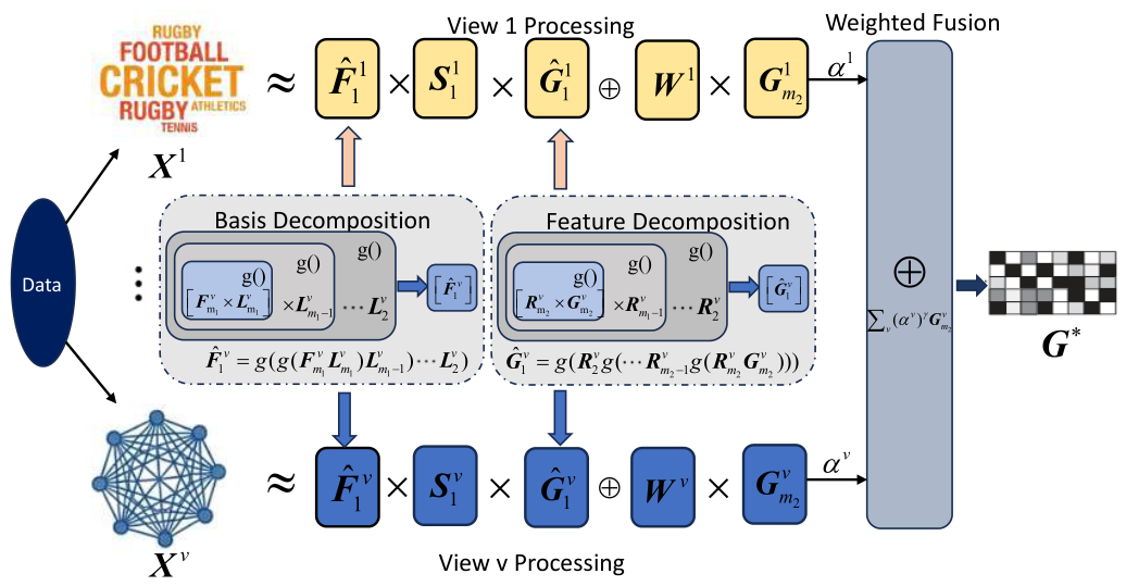
In the multi-view setting, we denote $\mathbf{X}=\{{\mathbf{X}}^1,\cdots$, ${\mathbf{X}}^V\}$ as the input data. As illustrated in Figure 2, GDNMF-MRL learns hierarchical representations by simultaneously decomposing both feature matrices and basis matrices across multiple views. From (6), we can naturally extend GDNMF as follows:

$$\begin{array}{cc}\hfill \underset{{\mathbf{F}}_1^v,{\mathbf{S}}_1^v,{\mathbf{G}}_1^v,{\mathbf{G}}_{m_2}^v,{\mathbf{W}}^v\ge 0}{\min }& \mathcal{O}=\sum _{v=1}^V\left(\parallel {\mathbf{X}}^v-{\widehat{\mathbf{F}}}_1^v{\mathbf{S}}_1^v{\widehat{\mathbf{G}}}_1^v-{\mathbf{W}}^v{\mathbf{G}}_{m_2}^v{\parallel }_F^2+\lambda \mathrm{tr}\left({\mathbf{G}}_{m_2}^v{\mathbf{L}}^v{\mathbf{G}}_{m_2}^{vT}\right)\right),\hfill \\ \hfill \mathrm{s}.\mathrm{t}.& {\widehat{\mathbf{F}}}_1^v=g\left(g\left(g\left({\mathbf{F}}_{m_1}^v{\mathbf{L}}_{m_1}^v\right){\mathbf{L}}_{m_1-1}^v\right)\cdots {\mathbf{L}}_2^v\right),\hfill \\ \hfill & {\widehat{\mathbf{G}}}_1^v=g\left({\mathbf{R}}_2^{v}g(\cdots {\mathbf{R}}_{m_2-1}^{v}g\left({\mathbf{R}}_{m_2}^v{\mathbf{G}}_{m_2}^v\right))\right),\hfill \end{array}$$

(7)

where ${\mathbf{L}}^v$ denotes the graph Laplacian matrix ${\mathbf{L}}^v={\mathbf{D}}^v-{\mathbf{A}}^v$, and ${\mathbf{D}}^v$ is a diagonal matrix whose entries are the row sums of ${\mathbf{A}}^v$, i.e., ${\mathbf{D}}_{jj}^v={\sum }_q{\mathbf{A}}_{jq}^v$.

We assume that although different views describe the data from heterogeneous perspectives, the underlying semantic patterns across views should be mutually compatible rather than contradictory. In other words, each view contains both view-specific information and shared latent structures that reflect the intrinsic characteristics of the data. Therefore, an effective multi-view model should not only preserve the individuality of each view, but also explicitly encourage consistency among their latent representations.

Motivated by this observation, we aim to explore the relevance of each view by learning a set of adaptive view weights, while simultaneously enforcing the latent representations of all views to align with a common representation. Let ${\mathbf{G}}^{*}$ denote the consensus latent representation shared by all views. To this end, the multi-view fusion term is formulated as

$$\begin{array}{cc}\hfill \underset{{\mathbf{G}}^{*},{\alpha }^v}{\min }& \mathcal{O}=\sum _{v=1}^V{\left({\alpha }^v\right)}^{\gamma }{\parallel {\mathbf{G}}_{m_2}^v-{\mathbf{G}}^{*}\parallel }_F^2\hfill \\ \hfill \mathrm{s}.\mathrm{t}.& {\mathbf{G}}^{*}\ge 0,\sum _{v=1}^V{\alpha }^v=1,\hfill \end{array}$$

(8)

where ${\mathbf{G}}_{m_2}^v$ denotes the latent representation learned from the v-th view, ${\alpha }^v$ is the corresponding view weight reflecting its contribution to the consensus representation, and $\gamma$ is a hyperparameter that controls the distribution of view weights. Specifically, a larger value of $\gamma$ encourages a more balanced weighting across views, whereas a smaller value allows the model to emphasize more informative views. By minimizing the weighted distances between individual view representations and the common representation, the proposed fusion term effectively promotes cross-view consistency while adaptively accounting for the relative importance of each view.

Therefore, considering both aspects mentioned above, the proposed GDNMF-MRL can be finally formulated as:

$$\begin{array}{cc}\hfill \underset{\begin{array}{c}{\mathbf{F}}_1^v,{\mathbf{S}}_1^v,{\mathbf{G}}_1^v,{\mathbf{G}}_{m_2}^v,\\ {\mathbf{G}}^{*},{\mathbf{W}}^v,\alpha \end{array}}{\min }\mathcal{O}& =\sum _{v=1}^V({\parallel {\mathbf{X}}^v-{\widehat{\mathbf{F}}}_1^v{\mathbf{S}}_1^v{\widehat{\mathbf{G}}}_1^v-{\mathbf{W}}^v{\mathbf{G}}_{m_2}^v\parallel }_F^2\hfill \\ \hfill & +\lambda \mathrm{tr}\left({\mathbf{G}}_{m_2}^v{\mathbf{L}}^v{\mathbf{G}}_{m_2}^{vT}\right)\hfill \\ \hfill & +{\left({\alpha }^v\right)}^{\gamma }{\parallel {\mathbf{G}}_{m_2}^v-{\mathbf{G}}^{*}\parallel }_F^2),\hfill \\ \hfill \mathrm{s}.\mathrm{t}.{\widehat{\mathbf{F}}}_1^v& =g\left(g\left(g\left({\mathbf{F}}_{m_1}^v{\mathbf{L}}_{m_1}^v\right){\mathbf{L}}_{m_1-1}^v\right)\cdots {\mathbf{L}}_2^v\right),\hfill \\ \hfill {\widehat{\mathbf{G}}}_1^v& =g\left({\mathbf{R}}_2^{v}g(\cdots {\mathbf{R}}_{m_2-1}^{v}g\left({\mathbf{R}}_{m_2}^v{\mathbf{G}}_{m_2}^v\right))\right),\hfill \\ \hfill {\mathbf{F}}_1^v,& {\mathbf{S}}_1^v,{\mathbf{G}}_1^v,{\mathbf{G}}_{m_2}^v,{\mathbf{G}}^{*},{\mathbf{W}}^v\ge 0,\sum _{v=1}^V{\alpha }^v=1.\hfill \end{array}$$

(9)

In our objective function, the first term consists of two complementary components: ${\widehat{\mathbf{F}}}_1^v{\mathbf{S}}_1^v{\widehat{\mathbf{G}}}_1^v$ and ${\mathbf{W}}^v{\mathbf{G}}_{m_2}^v$. Specifically, ${\widehat{\mathbf{F}}}_1^v{\mathbf{S}}_1^v{\widehat{\mathbf{G}}}_1^v$ is obtained via a deep nonlinear model to capture complex hierarchical and nonlinear structures, while ${\mathbf{W}}^v{\mathbf{G}}_{m_2}^v$ is modeled by a shallow linear framework to preserve linear information, where ${\mathbf{W}}^v$ denotes the linear basis matrix. When the nonlinear component is removed, GDNMF-MRL degenerates into a conventional NMF model applicable to multi-view data. Conversely, when the linear component is omitted and the feature matrix decomposition layer or the basis matrix decomposition layer is restricted to one, GDNMF-MRL reduces to DSNMF-MRL or DNBMF-MRL, respectively, extending DSNMF and DNBMF to the multi-view setting. In this sense, GDNMF-MRL provides a unified and generalized framework that encompasses various existing NMF and deep NMF models, offering high flexibility for diverse practical scenarios. The second term is a graph regularization term designed to preserve the intrinsic geometric structure of the original data. Moreover, the third term integrates multiple ${\mathbf{G}}_{m_2}^v$ to learn an updated consensus representation ${\mathbf{G}}^{*}$.

3.2. One-Step GDNMF-MRL

Although the GDNMF-MRL model introduced in Section 3.1 achieves competitive clustering performance for multi-view representation learning, it adopts a two-stage strategy: first learning a consensus representation matrix ${\mathbf{G}}^{*}$, and then applying the k-means algorithm to obtain clustering labels. Since representation learning and clustering are optimized independently, the lack of direct interaction between these two stages may restrict the model from fully exploiting the latent clustering structure.

To overcome this drawback, we propose a one-step GDNMF-MRL framework (OS-GDNMF-MRL) that directly integrates discrete label learning into the representation learning process. In traditional k-means clustering, the objective is to partition the learned representation ${\mathbf{G}}^{*}$ into K clusters by minimizing the reconstruction error with respect to cluster centroids, which can be formulated as

$$\begin{array}{cc}\hfill \underset{\mathbf{F},\mathbf{Y}}{\min }& \parallel {\mathbf{G}}^{*}{-\mathbf{F}\mathbf{Y}\parallel }_F^2,\hfill \\ \hfill \mathrm{s}.\mathrm{t}.& Y_{kj}\in \{0,1\},\sum _{k=1}^K{Y}_{kj}=1\forall j=1,\dots ,n,\hfill \end{array}$$

(10)

where $\mathbf{F}\in {\mathbb{R}}^{K\times K}$ denotes the centroid matrix and $\mathbf{Y}\in {\mathbb{R}}^{K\times n}$ is the cluster indicator matrix.

Motivated by this formulation, we construct a one-step multi-view fusion term by jointly considering representation alignment and clustering assignment, leading to

$$\begin{array}{cc}\hfill \underset{{\mathbf{F}}^v,\mathbf{Y},{\alpha }^v}{\min }& \sum _{v=1}^V{\left({\alpha }^v\right)}^{\gamma }{\parallel {\mathbf{G}}_{m_2}^v-{\mathbf{F}}^v\mathbf{Y}\parallel }_F^2,\hfill \\ \hfill \mathrm{s}.\mathrm{t}.& \sum _{v=1}^V{\alpha }^v=1,Y_{kj}\in \{0,1\},\sum _{k=1}^K{Y}_{kj}=1\forall j=1,\dots ,n.\hfill \end{array}$$

(11)

Considering that multi-view clustering aims to produce a unified partition of samples, we introduce view-specific centroid matrices ${\mathbf{F}}^v$ while enforcing a shared cluster indicator matrix $\mathbf{Y}$ across all views. By embedding this one-step fusion mechanism into the original GDNMF objective, we obtain the proposed OS-GDNMF-MRL model, whose overall optimization problem is given by

$$\begin{array}{cc}\hfill \underset{\begin{array}{c}{\mathbf{F}}_1^v,{\mathbf{S}}_1^v,{\mathbf{G}}_{m_2}^v,{\mathbf{F}}^v,\mathbf{Y},{\alpha }^v\end{array}}{\min }\mathcal{O}& =\sum _{v=1}^V({\parallel {\mathbf{X}}^v-{\widehat{\mathbf{F}}}_1^v{\mathbf{S}}_1^v{\widehat{\mathbf{G}}}_1^v-{\mathbf{W}}^v{\mathbf{G}}_{m_2}^v\parallel }_F^2\hfill \\ \hfill & +\lambda \mathrm{tr}\left({\mathbf{G}}_{m_2}^v{\mathbf{L}}^v{\left({\mathbf{G}}_{m_2}^v\right)}^T\right)\hfill \\ \hfill & +{\left({\alpha }^v\right)}^{\gamma }{\parallel {\mathbf{G}}_{m_2}^v-{\mathbf{F}}^v\mathbf{Y}\parallel }_F^2),\hfill \\ \hfill \mathrm{s}.\mathrm{t}.& {\mathbf{F}}_1^v,{\mathbf{S}}_1^v,{\mathbf{G}}_{m_2}^v,{\mathbf{F}}^v\ge 0,\hfill \\ \hfill & \sum _{v=1}^V{\alpha }^v=1,\hfill \\ \hfill & Y_{kj}\in \{0,1\},\sum _{k=1}^K{Y}_{kj}=1,\forall j=1,\dots ,n.\hfill \end{array}$$

(12)

Compared with the original GDNMF-MRL, the proposed OS-GDNMF-MRL jointly optimizes deep representation learning and clustering assignment within a unified framework, without introducing additional hyperparameters. Different from conventional approaches that perform clustering as a post-processing step after representation learning, OS-GDNMF-MRL integrates the clustering indicator matrix $\mathbf{Y}$ directly into the objective function and jointly optimizes representation and clustering variables in an alternating manner. By explicitly coupling representation learning with clustering, the model can better exploit latent cluster structures, resulting in more discriminative subspace representations and improved clustering accuracy.

4. Optimization

In this section, we present the optimization procedures for both the GDNMF-MRL and OS-GDNMF-MRL models, and provide a computational complexity analysis.

4.1. GDNMF-MRL Optimization

In this subsection, we introduce the optimization algorithm for GDNMF-MRL in Equation (9). The algorithm consists of two phases: pre-training and fine-tuning. For pre-training, we independently solve the subproblems of all layers. Then, we initialize the model in Equation (9) through pre-training and fine-tune it using an alternating algorithm with gradient backpropagation.

In the pre-training phase, for basis decomposition, we iteratively solve the following subproblems layer by layer:

$$\underset{{\mathbf{F}}_{i+1}^v,{\mathbf{L}}_{i+1}^v\ge 0}{\min }{\displaystyle \frac{1}{2}}{\parallel {\mathbf{F}}_i^v-g\left({\mathbf{F}}_{i+1}^v{\mathbf{L}}_{i+1}^v\right)\parallel }_F^2.$$

(13)

Here, we assume that the nonlinear mapping $g(·)$ is invertible, and that $g(·)$, $g^{-1}(·)$, and $g^{\prime }(·)$ are applied element-wise to matrices.

This is a non-convex problem with non-negative constraints; thus, we fix one factor and update the other alternately. To make the derivation explicit, let ${\mathbf{Z}}_{i+1}^v=g^{-1}\left({\mathbf{F}}_i^v\right)$. Then Equation (13) is equivalently rewritten as

$$\underset{{\mathbf{F}}_{i+1}^v,{\mathbf{L}}_{i+1}^v\ge 0}{\min }{\displaystyle \frac{1}{2}}{\parallel {\mathbf{Z}}_{i+1}^v-{\mathbf{F}}_{i+1}^v{\mathbf{L}}_{i+1}^v\parallel }_F^2.$$

(14)

Accordingly, the partial derivatives with respect to the two factors are

$${\displaystyle \frac{\partial \mathcal{O}}{\partial {\mathbf{F}}_{i+1}^v}}={\mathbf{F}}_{i+1}^v{\mathbf{L}}_{i+1}^v{\left({\mathbf{L}}_{i+1}^v\right)}^T-{\mathbf{Z}}_{i+1}^v{\left({\mathbf{L}}_{i+1}^v\right)}^T,$$

(15)

$${\displaystyle \frac{\partial \mathcal{O}}{\partial {\mathbf{L}}_{i+1}^v}}={\left({\mathbf{F}}_{i+1}^v\right)}^T{\mathbf{F}}_{i+1}^v{\mathbf{L}}_{i+1}^v-{\left({\mathbf{F}}_{i+1}^v\right)}^T{\mathbf{Z}}_{i+1}^v.$$

(16)

Using the KKT complementary conditions for the non-negative constraints, we express the gradient as the difference between its positive and negative parts. This allows us to derive the multiplicative update rules by enforcing the element-wise complementary condition.

$${\mathbf{F}}_{i+1}^v={\mathbf{F}}_{i+1}^v\odot {\displaystyle \frac{g^{-1}\left({\mathbf{F}}_i^v\right){\left({\mathbf{L}}_{i+1}^v\right)}^T}{{\mathbf{F}}_{i+1}^v{\mathbf{L}}_{i+1}^v{\left({\mathbf{L}}_{i+1}^v\right)}^T}}.$$

(17)

$${\mathbf{L}}_{i+1}^v={\mathbf{L}}_{i+1}^v\odot {\displaystyle \frac{{\left({\mathbf{F}}_{i+1}^v\right)}^T{g}^{-1}\left({\mathbf{F}}_i^v\right)}{{\left({\mathbf{F}}_{i+1}^v\right)}^T{\mathbf{F}}_{i+1}^v{\mathbf{L}}_{i+1}^v}}.$$

(18)

For feature decomposition, we independently solve a similar subproblem at layer i, i.e.,

$$\underset{{\mathbf{G}}_{i+1}^v,{\mathbf{R}}_{i+1}^v\ge 0}{\min }{\displaystyle \frac{1}{2}}{\parallel {\mathbf{G}}_i^v-g\left({\mathbf{R}}_{i+1}^v{\mathbf{G}}_{i+1}^v\right)\parallel }_F^2.$$

(19)

Similarly, let ${\mathbf{Q}}_{i+1}^v=g^{-1}\left({\mathbf{G}}_i^v\right)$. Then Equation (19) becomes

$$\underset{{\mathbf{G}}_{i+1}^v,{\mathbf{R}}_{i+1}^v\ge 0}{\min }{\displaystyle \frac{1}{2}}{\parallel {\mathbf{Q}}_{i+1}^v-{\mathbf{R}}_{i+1}^v{\mathbf{G}}_{i+1}^v\parallel }_F^2.$$

(20)

The corresponding partial derivatives are

$${\displaystyle \frac{\partial \mathcal{O}}{\partial {\mathbf{R}}_{i+1}^v}}={\mathbf{R}}_{i+1}^v{\mathbf{G}}_{i+1}^v{\left({\mathbf{G}}_{i+1}^v\right)}^T-{\mathbf{Q}}_{i+1}^v{\left({\mathbf{G}}_{i+1}^v\right)}^T,$$

(21)

$${\displaystyle \frac{\partial \mathcal{O}}{\partial {\mathbf{G}}_{i+1}^v}}={\left({\mathbf{R}}_{i+1}^v\right)}^T{\mathbf{R}}_{i+1}^v{\mathbf{G}}_{i+1}^v-{\left({\mathbf{R}}_{i+1}^v\right)}^T{\mathbf{Q}}_{i+1}^v.$$

(22)

Applying the same KKT-based multiplicative update strategy yields

$${\mathbf{R}}_{i+1}^v={\mathbf{R}}_{i+1}^v\odot {\displaystyle \frac{g^{-1}\left({\mathbf{G}}_i^v\right){\left({\mathbf{G}}_{i+1}^v\right)}^T}{{\mathbf{R}}_{i+1}^v{\mathbf{G}}_{i+1}^v{\left({\mathbf{G}}_{i+1}^v\right)}^T}}.$$

(23)

$${\mathbf{G}}_{i+1}^v={\mathbf{G}}_{i+1}^v\odot {\displaystyle \frac{{\left({\mathbf{R}}_{i+1}^v\right)}^T{g}^{-1}\left({\mathbf{G}}_i^v\right)}{{\left({\mathbf{R}}_{i+1}^v\right)}^T{\mathbf{R}}_{i+1}^v{\mathbf{G}}_{i+1}^v}}.$$

(24)

In the fine-tuning phase, the optimization problem of GDNMF-MRL in Equation (9) is solved based on alternating optimization. Let $\mathcal{O}$ denote the objective value in Equation (9). To improve reproducibility, we next give the intermediate chain-rule expansions used to derive the gradients and then state the corresponding variable updates. The algorithm repeats the following steps until convergence.

Update ${\mathbf{F}}_i^v$: To optimize $\mathcal{O}$ with respect to ${\mathbf{F}}_i^v$, we first consider the following sub-problem:

$$\begin{array}{cc}\hfill \underset{{\mathbf{F}}_i^v\ge 0}{\min }& {\mathcal{O}}_{\mathrm{obj}}\left({\mathbf{F}}_i^v\right)={\displaystyle \frac{1}{2}}{\parallel {\mathbf{X}}^v-{\widehat{\mathbf{F}}}_1^v{\mathbf{S}}_1^v{\widehat{\mathbf{G}}}_1^v-{\mathbf{W}}^v{\mathbf{G}}_{m_2}^v\parallel }_F^2,\hfill \\ \hfill \mathrm{s}.\mathrm{t}.& {\mathbf{F}}_{i-1}^v=g\left({\mathbf{F}}_i^v{\mathbf{L}}_i^v\right),i=2,\dots ,m_1.\hfill \end{array}$$

(25)

Based on the chain rule, the gradient with respect to the i-th basis layer is derived as

$$\begin{array}{cc}\hfill {\nabla }_{{\mathbf{F}}_i^v}\mathcal{O}& ={\displaystyle \frac{\partial {\mathcal{O}}_{\mathrm{obj}}}{\partial {\mathbf{F}}_i^v}}={\displaystyle \frac{\partial {\mathcal{O}}_{\mathrm{obj}}}{\partial {\mathbf{F}}_i^v{\mathbf{L}}_i^v}}{\left({\mathbf{L}}_i^v\right)}^T\hfill \\ \hfill & =\left[{\displaystyle \frac{\partial {\mathcal{O}}_{\mathrm{obj}}}{\partial g\left({\mathbf{F}}_i^v{\mathbf{L}}_i^v\right)}}\odot g^{\prime }\left({\mathbf{F}}_i^v{\mathbf{L}}_i^v\right)\right]{\left({\mathbf{L}}_i^v\right)}^T\hfill \\ \hfill & =[{\nabla }_{{\mathbf{F}}_{i-1}^v}\mathcal{O}\odot g^{\prime }\left({\mathbf{F}}_i^v{\mathbf{L}}_i^v\right)]{\left({\mathbf{L}}_i^v\right)}^T.\hfill \end{array}$$

(26)

For the first layer, the corresponding sub-problem is

$$\begin{array}{cc}\hfill \underset{{\mathbf{F}}_1^v\ge 0}{\min }& {\displaystyle \frac{1}{2}}{\parallel {\mathbf{X}}^v-{\mathbf{F}}_1^v{\mathbf{S}}_1^v{\mathbf{G}}_1^v-{\mathbf{W}}^v{\mathbf{G}}_{m_2}^v\parallel }_F^2.\hfill \end{array}$$

(27)

Thus, its derivative is

$${\nabla }_{{\mathbf{F}}_1^v}\mathcal{O}=-({\mathbf{X}}^v-{\mathbf{F}}_1^v{\mathbf{S}}_1^v{\mathbf{G}}_1^v-{\mathbf{W}}^v{\mathbf{G}}_{m_2}^v){\mathbf{G}}_1^{vT}{\mathbf{S}}_1^{vT}.$$

(28)

Update ${\mathbf{R}}_i^v$, ${\mathbf{L}}_i^v$, and ${\mathbf{S}}_1^v$: For ${\mathbf{L}}_i^v$ and ${\mathbf{R}}_i^v$, we similarly optimize each variable while fixing the others. In particular, the sub-problem for ${\mathbf{L}}_i^v$ is

$$\begin{array}{cc}\hfill \underset{{\mathbf{L}}_i^v\ge 0}{\min }& {\mathcal{O}}_{\mathrm{obj}}\left({\mathbf{L}}_i^v\right)={\displaystyle \frac{1}{2}}{\parallel {\mathbf{X}}^v-{\widehat{\mathbf{F}}}_1^v{\mathbf{S}}_1^v{\widehat{\mathbf{G}}}_1^v-{\mathbf{W}}^v{\mathbf{G}}_{m_2}^v\parallel }_F^2,\hfill \\ \hfill \mathrm{s}.\mathrm{t}.& {\mathbf{F}}_{i-1}^v=g\left({\mathbf{F}}_i^v{\mathbf{L}}_i^v\right),i=2,\dots ,m_1,\hfill \end{array}$$

(29)

which gives

$$\begin{array}{cc}\hfill {\nabla }_{{\mathbf{L}}_i^v}\mathcal{O}& ={\displaystyle \frac{\partial \mathcal{O}}{\partial {\mathbf{L}}_i^v}}={\mathbf{F}}_i^{vT}{\displaystyle \frac{\partial \mathcal{O}}{\partial {\mathbf{F}}_i^v{\mathbf{L}}_i^v}}\hfill \\ \hfill & ={\mathbf{F}}_i^{vT}\left[{\displaystyle \frac{\partial \mathcal{O}}{\partial g\left({\mathbf{F}}_i^v{\mathbf{L}}_i^v\right)}}\odot g^{\prime }\left({\mathbf{F}}_i^v{\mathbf{L}}_i^v\right)\right]\hfill \\ \hfill & ={\mathbf{F}}_i^{vT}[{\nabla }_{{\mathbf{F}}_{i-1}^v}\mathcal{O}\odot g^{\prime }\left({\mathbf{F}}_i^v{\mathbf{L}}_i^v\right)].\hfill \end{array}$$

(30)

The sub-problem for ${\mathbf{R}}_i^v$ is

$$\begin{array}{cc}\hfill \underset{{\mathbf{R}}_i^v\ge 0}{\min }& {\mathcal{O}}_{\mathrm{obj}}\left({\mathbf{R}}_i^v\right)={\displaystyle \frac{1}{2}}{\parallel {\mathbf{X}}^v-{\widehat{\mathbf{F}}}_1^v{\mathbf{S}}_1^v{\widehat{\mathbf{G}}}_1^v-{\mathbf{W}}^v{\mathbf{G}}_{m_2}^v\parallel }_F^2,\hfill \\ \hfill \mathrm{s}.\mathrm{t}.& {\mathbf{G}}_{i-1}^v=g\left({\mathbf{R}}_i^v{\mathbf{G}}_i^v\right),i=2,\dots ,m_2,\hfill \end{array}$$

(31)

and its gradient is

$$\begin{array}{cc}\hfill {\nabla }_{{\mathbf{R}}_i^v}\mathcal{O}& ={\displaystyle \frac{\partial \mathcal{O}}{\partial {\mathbf{R}}_i^v}}={\displaystyle \frac{\partial \mathcal{O}}{\partial {\mathbf{R}}_i^v{\mathbf{G}}_i^v}}{\mathbf{G}}_i^{vT}\hfill \\ \hfill & =\left[{\displaystyle \frac{\partial \mathcal{O}}{\partial g\left({\mathbf{R}}_i^v{\mathbf{G}}_i^v\right)}}\odot g^{\prime }\left({\mathbf{R}}_i^v{\mathbf{G}}_i^v\right)\right]{\mathbf{G}}_i^{vT}\hfill \\ \hfill & =[{\nabla }_{{\mathbf{G}}_{i-1}^v}\mathcal{O}\odot g^{\prime }\left({\mathbf{R}}_i^v{\mathbf{G}}_i^v\right)]{\mathbf{G}}_i^{vT}.\hfill \end{array}$$

(32)

For ${\mathbf{S}}_1^v$, we solve

$$\begin{array}{cc}\hfill \underset{{\mathbf{S}}_1^v\ge 0}{\min }& {\mathcal{O}}_{\mathrm{obj}}\left({\mathbf{S}}_1^v\right)={\displaystyle \frac{1}{2}}{\parallel {\mathbf{X}}^v-{\mathbf{F}}_1^v{\mathbf{S}}_1^v{\mathbf{G}}_1^v-{\mathbf{W}}^v{\mathbf{G}}_{m_2}^v\parallel }_F^2,\hfill \end{array}$$

(33)

which yields

$${\nabla }_{{\mathbf{S}}_1^v}\mathcal{O}=-{\mathbf{F}}_1^{vT}({\mathbf{X}}^v-{\mathbf{F}}_1^v{\mathbf{S}}_1^v{\mathbf{G}}_1^v-{\mathbf{W}}^v{\mathbf{G}}_{m_2}^v){\mathbf{G}}_1^{vT}.$$

(34)

Update ${\mathbf{G}}^v$: For ${\mathbf{G}}_1^v$, we solve the first-layer sub-problem

$$\begin{array}{cc}\hfill \underset{{\mathbf{G}}_1^v\ge 0}{\min }& {\mathcal{O}}_{\mathrm{obj}}\left({\mathbf{G}}_1^v\right)={\displaystyle \frac{1}{2}}{\parallel {\mathbf{X}}^v-{\mathbf{F}}_1^v{\mathbf{S}}_1^v{\mathbf{G}}_1^v-{\mathbf{W}}^v{\mathbf{G}}_{m_2}^v\parallel }_F^2,\hfill \end{array}$$

(35)

which yields

$${\nabla }_{{\mathbf{G}}_1^v}\mathcal{O}=-{\left({\mathbf{F}}_1^v{\mathbf{S}}_1^v\right)}^T({\mathbf{X}}^v-{\mathbf{F}}_1^v{\mathbf{S}}_1^v{\mathbf{G}}_1^v-{\mathbf{W}}^v{\mathbf{G}}_{m_2}^v).$$

(36)

For intermediate layers, i.e., $1<i<m_2$, the corresponding sub-problem is

$$\begin{array}{cc}\hfill \underset{{\mathbf{G}}_i^v\ge 0}{\min }& {\mathcal{O}}_{\mathrm{obj}}\left({\mathbf{G}}_i^v\right)={\displaystyle \frac{1}{2}}{\parallel {\mathbf{X}}^v-{\widehat{\mathbf{F}}}_1^v{\mathbf{S}}_1^v{\widehat{\mathbf{G}}}_1^v-{\mathbf{W}}^v{\mathbf{G}}_{m_2}^v\parallel }_F^2,\hfill \\ \hfill \mathrm{s}.\mathrm{t}.& {\mathbf{G}}_{i-1}^v=g\left({\mathbf{R}}_i^v{\mathbf{G}}_i^v\right),i=2,\dots ,m_2-1,\hfill \end{array}$$

(37)

and the gradient is

$$\begin{array}{cc}\hfill {\nabla }_{{\mathbf{G}}_i^v}\mathcal{O}& ={\displaystyle \frac{\partial \mathcal{O}}{\partial {\mathbf{G}}_i^v}}={\left({\mathbf{R}}_i^v\right)}^T{\displaystyle \frac{\partial \mathcal{O}}{\partial {\mathbf{R}}_i^v{\mathbf{G}}_i^v}}\hfill \\ \hfill & ={\left({\mathbf{R}}_i^v\right)}^T\left[{\displaystyle \frac{\partial \mathcal{O}}{\partial g\left({\mathbf{R}}_i^v{\mathbf{G}}_i^v\right)}}\odot g^{\prime }\left({\mathbf{R}}_i^v{\mathbf{G}}_i^v\right)\right]\hfill \\ \hfill & ={\left({\mathbf{R}}_i^v\right)}^T[{\nabla }_{{\mathbf{G}}_{i-1}^v}\mathcal{O}\odot g^{\prime }\left({\mathbf{R}}_i^v{\mathbf{G}}_i^v\right)].\hfill \end{array}$$

(38)

For the last feature layer, i.e., $i=m_2$, we consider

$$\begin{array}{cc}\hfill \underset{{\mathbf{G}}_{m_2}^v\ge 0}{\min }{\mathcal{O}}_{\mathrm{obj}}\left({\mathbf{G}}_{m_2}^v\right)& ={\displaystyle \frac{1}{2}}{\parallel {\mathbf{X}}^v-{\widehat{\mathbf{F}}}_1^v{\mathbf{S}}_1^v{\widehat{\mathbf{G}}}_1^v-{\mathbf{W}}^v{\mathbf{G}}_{m_2}^v\parallel }_F^2\hfill \\ \hfill & +\lambda \mathrm{tr}\left({\mathbf{G}}_{m_2}^v{\mathbf{L}}^v{\mathbf{G}}_{m_2}^{vT}\right)+{\left({\alpha }^v\right)}^{\gamma }{\parallel {\mathbf{G}}_{m_2}^v-{\mathbf{G}}^{*}\parallel }_F^2,\hfill \end{array}$$

(39)

which gives

$$\begin{array}{cc}\hfill {\nabla }_{{\mathbf{G}}_{m_2}^v}\mathcal{O}& ={\left({\mathbf{R}}_{m_2}^v\right)}^T[{\nabla }_{{\mathbf{G}}_{m_2-1}^v}\mathcal{O}\odot g^{\prime }\left({\mathbf{R}}_{m_2}^v{\mathbf{G}}_{m_2}^v\right)]\hfill \\ \hfill & -{\mathbf{W}}^{vT}({\mathbf{X}}^v-{\mathbf{F}}_1^v{\mathbf{S}}_1^v{\mathbf{G}}_1^v-{\mathbf{W}}^v{\mathbf{G}}_{m_2}^v)\hfill \\ \hfill & -\lambda {\mathbf{G}}_{m_2}^v{\mathbf{L}}^v-(1+{\left({\alpha }^v\right)}^{\gamma }){\mathbf{G}}_{m_2}^v-{\left({\alpha }^v\right)}^{\gamma }{\mathbf{G}}^{*}.\hfill \end{array}$$

(40)

Update ${\mathbf{W}}^v$: By fixing the remaining variables, the sub-problem with respect to ${\mathbf{W}}^v$ can be written as

$$\begin{array}{cc}\hfill \underset{{\mathbf{W}}^v\ge 0}{\min }& {\mathcal{O}}_{\mathrm{obj}}\left({\mathbf{W}}^v\right)={\displaystyle \frac{1}{2}}{\parallel {\mathbf{X}}^v-{\widehat{\mathbf{F}}}_1^v{\mathbf{S}}_1^v{\widehat{\mathbf{G}}}_1^v-{\mathbf{W}}^v{\mathbf{G}}_{m_2}^v\parallel }_F^2.\hfill \end{array}$$

(41)

Taking the derivative with respect to ${\mathbf{W}}^v$ yields

$${\nabla }_{{\mathbf{W}}^v}\mathcal{O}=-({\mathbf{X}}^v-{\mathbf{F}}_1^v{\mathbf{S}}_1^v{\mathbf{G}}_1^v-{\mathbf{W}}^v{\mathbf{G}}_{m_2}^v){\mathbf{G}}_{m_2}^{vT}.$$

(42)

Update ${\mathbf{G}}^{*}$: By fixing ${\left\{{\mathbf{G}}_{m_2}^v\right\}}_{v=1}^V$ and ${\left\{{\alpha }^v\right\}}_{v=1}^V$, the optimization problem for the consensus representation becomes

$$\underset{{\mathbf{G}}^{*}\ge 0}{\min }\sum _{v=1}^V{\left({\alpha }^v\right)}^{\gamma }{\parallel {\mathbf{G}}_{m_2}^v-{\mathbf{G}}^{*}\parallel }_F^2.$$

(43)

Setting the derivative with respect to ${\mathbf{G}}^{*}$ to zero gives

$$\sum _{v=1}^V{\left({\alpha }^v\right)}^{\gamma }({\mathbf{G}}^{*}-{\mathbf{G}}_{m_2}^v)=0,$$

(44)

from which we obtain

$${\mathbf{G}}^{*}={\displaystyle \frac{{\sum }_{v=1}^V{\left({\alpha }^v\right)}^{\gamma }{\mathbf{G}}_{m_2}^v}{{\sum }_{v=1}^V{\left({\alpha }^v\right)}^{\gamma }}}.$$

(45)

Update ${\alpha }^v$: By fixing ${\mathbf{G}}_{m_2}^v$ and ${\mathbf{G}}^{*}$, the optimization with respect to the view weights is reduced to

$$\underset{{\alpha }^v}{\min }\sum _{v=1}^V{\left({\alpha }^v\right)}^{\gamma }{\parallel {\mathbf{G}}_{m_2}^v-{\mathbf{G}}^{*}\parallel }_F^2,\mathrm{s}.\mathrm{t}.\sum _{v=1}^V{\alpha }^v=1.$$

(46)

Let $P^v={\parallel {\mathbf{P}}^v\parallel }_F^2$ with ${\mathbf{P}}^v={\mathbf{G}}_{m_2}^v-{\mathbf{G}}^{*}$. By introducing a Lagrange multiplier for the simplex constraint and solving the stationary condition, we obtain

$${\alpha }^v={\displaystyle \frac{{\left(P^v\right)}^{\frac{1}{1-\gamma }}}{{\sum }_{v=1}^V{\left(P^v\right)}^{\frac{1}{1-\gamma }}}},P^v={\parallel {\mathbf{P}}^v\parallel }_F^2,{\mathbf{P}}^v={\mathbf{G}}_{m_2}^v-{\mathbf{G}}^{*}.$$

(47)

4.2. OS-GDNMF-MRL Optimization

This subsection focuses on the optimization procedure of the proposed OS-GDNMF-MRL model. Specifically, the update strategies for most variables remain identical to those adopted in the original GDNMF-MRL framework, except for the representation matrix ${\mathbf{G}}_{m_2}^v$, the view-specific centroid matrix ${\mathbf{F}}^v$, the clustering indicator matrix $\mathbf{Y}$, and the view weight ${\alpha }^v$. As a result, only the optimization rules associated with these variables are elaborated in the following, while the remaining update steps follow the same scheme as in GDNMF-MRL.

(1) Update rule for representation matrix ${\mathbf{G}}_{m_2}^v$: Fixing other variables, the optimization problem for updating variable ${\mathbf{G}}_{m_2}^v$ can be rewritten as

$$\begin{array}{cc}\hfill \mathcal{O}\left({\mathbf{G}}_{m_2}^v\right)& =\mathrm{tr}({\mathbf{G}}_{m_2}^v{\mathbf{G}}_{m_2}^{vT}+{\mathbf{G}}_{m_2}^v{\left({\mathbf{W}}^v\right)}^T{\mathbf{W}}^v{\mathbf{G}}_{m_2}^{vT}\hfill \\ \hfill & -2{\left({\mathbf{X}}^v\right)}^T{\mathbf{W}}^v{\mathbf{G}}_{m_2}^{vT}+\lambda {\mathbf{G}}_{m_2}^v{\mathbf{L}}^v{\mathbf{G}}_{m_2}^{vT}\hfill \\ \hfill & +{\left({\alpha }^v\right)}^{\gamma }{({\mathbf{G}}_{m_2}^v-{\mathbf{F}}^v\mathbf{Y})}^T({\mathbf{G}}_{m_2}^v-{\mathbf{F}}^v\mathbf{Y})),\hfill \\ \hfill \mathrm{s}.\mathrm{t}.& {\mathbf{G}}_{m_2}^v\ge 0.\hfill \end{array}$$

(48)

The update rule for ${\mathbf{G}}_{m_2}^v$ is formulated as follows. To make Equation (48) reproducible, we first expand Equation (48) term by term:

$$\begin{array}{cc}\hfill \mathcal{O}\left({\mathbf{G}}_{m_2}^v\right)& =\mathrm{tr}\left({\mathbf{G}}_{m_2}^v{\mathbf{G}}_{m_2}^{vT}\right)+\mathrm{tr}\left({\mathbf{G}}_{m_2}^v{\left({\mathbf{W}}^v\right)}^T{\mathbf{W}}^v{\mathbf{G}}_{m_2}^{vT}\right)\hfill \\ \hfill & -2\mathrm{tr}\left({\left({\mathbf{X}}^v\right)}^T{\mathbf{W}}^v{\mathbf{G}}_{m_2}^{vT}\right)+\lambda \mathrm{tr}\left({\mathbf{G}}_{m_2}^v{\mathbf{L}}^v{\mathbf{G}}_{m_2}^{vT}\right)\hfill \\ \hfill & +{\left({\alpha }^v\right)}^{\gamma }\mathrm{tr}({\mathbf{G}}_{m_2}^v{\mathbf{G}}_{m_2}^{vT}-2{\mathbf{G}}_{m_2}^v{\mathbf{Y}}^T{\left({\mathbf{F}}^v\right)}^T+{\mathbf{F}}^v\mathbf{Y}{\mathbf{Y}}^T{\left({\mathbf{F}}^v\right)}^T).\hfill \end{array}$$

(49)

By using standard matrix derivative identities, we obtain

$$\begin{array}{cc}\hfill {\displaystyle \frac{\partial \mathcal{O}}{\partial {\mathbf{G}}_{m_2}^v}}& =2{\mathbf{G}}_{m_2}^v+2{\left({\mathbf{W}}^v\right)}^T{\mathbf{W}}^v{\mathbf{G}}_{m_2}^v-2{\left({\mathbf{W}}^v\right)}^T{\mathbf{X}}^v\hfill \\ \hfill & +2\lambda {\mathbf{G}}_{m_2}^v{\mathbf{L}}^v+2{\left({\alpha }^v\right)}^{\gamma }{\mathbf{G}}_{m_2}^v-2{\left({\alpha }^v\right)}^{\gamma }{\mathbf{F}}^v\mathbf{Y}.\hfill \end{array}$$

(50)

Substituting ${\mathbf{L}}^v={\mathbf{D}}^v-{\mathbf{S}}^v$ gives

$$\begin{array}{cc}\hfill {\displaystyle \frac{1}{2}}{\displaystyle \frac{\partial \mathcal{O}}{\partial {\mathbf{G}}_{m_2}^v}}& ={\mathbf{G}}_{m_2}^v+{\left({\mathbf{W}}^v\right)}^T{\mathbf{W}}^v{\mathbf{G}}_{m_2}^v+\lambda {\mathbf{G}}_{m_2}^v{\mathbf{D}}^v+{\left({\alpha }^v\right)}^{\gamma }{\mathbf{G}}_{m_2}^v\hfill \\ \hfill & -\left({\left({\mathbf{W}}^v\right)}^T{\mathbf{X}}^v+\lambda {\mathbf{G}}_{m_2}^v{\mathbf{S}}^v+{\left({\alpha }^v\right)}^{\gamma }{\mathbf{F}}^v\mathbf{Y}\right).\hfill \end{array}$$

(51)

Combining this decomposition with the KKT complementary condition yields the multiplicative update

$$\begin{array}{cc}\hfill {\mathbf{G}}_{m_2}^v& ={\mathbf{G}}_{m_2}^v\odot {\displaystyle \frac{2{\left({\mathbf{W}}^v\right)}^T{\mathbf{X}}^v+\lambda {\mathbf{G}}_{m_2}^v{\mathbf{S}}^v+{\left({\alpha }^v\right)}^{\gamma }{\mathbf{F}}^v\mathbf{Y}}{{\mathbf{G}}_{m_2}^v+{\left({\mathbf{W}}^v\right)}^T{\mathbf{W}}^v{\mathbf{G}}_{m_2}^v+\lambda {\mathbf{G}}_{m_2}^v{\mathbf{D}}^v+(1+{\left({\alpha }^v\right)}^{\gamma }){\mathbf{G}}_{m_2}^v}}.\hfill \end{array}$$

(52)

(2) Update rule for centroid matrix ${\mathbf{F}}^v$: By fixing ${\mathbf{G}}_{m_2}^v$ and the clustering indicator matrix $\mathbf{Y}$, the optimization problem in Equation (26) with respect to ${\mathbf{F}}^v$ can be reduced to the following form:

$$\mathcal{O}\left({\mathbf{F}}^v\right)=\mathrm{tr}\left({\mathbf{Y}}^T{\mathbf{F}}^{vT}{\mathbf{F}}^v\mathbf{Y}-2{\mathbf{G}}_{m_2}^v{\mathbf{Y}}^T{\mathbf{F}}^{vT}\right).$$

(53)

Taking the derivative of $\mathcal{O}\left({\mathbf{F}}^v\right)$ with respect to ${\mathbf{F}}^v$ and setting it to zero yields a closed-form solution. Specifically,

$${\displaystyle \frac{\partial \mathcal{O}\left({\mathbf{F}}^v\right)}{\partial {\mathbf{F}}^v}}=2{\mathbf{F}}^v\mathbf{Y}{\mathbf{Y}}^T-2{\mathbf{G}}_{m_2}^v{\mathbf{Y}}^T.$$

(54)

Setting the above derivative to zero gives

$${\mathbf{F}}^v\mathbf{Y}{\mathbf{Y}}^T={\mathbf{G}}_{m_2}^v{\mathbf{Y}}^T,$$

(55)

and therefore

$${\mathbf{F}}^v={\mathbf{G}}_{m_2}^v{\mathbf{Y}}^T{\left(\mathbf{Y}{\mathbf{Y}}^T\right)}^{-1}.$$

(56)

(3) Update rule for clustering label matrix $\mathbf{Y}$: When ${\mathbf{G}}_{m_2}^v$ and ${\mathbf{F}}^v$ are fixed, the optimization problem in Equation (26) with respect to $\mathbf{Y}$ simplifies to

$$\begin{array}{cc}\hfill \underset{\mathbf{Y}}{\min }& \sum _{v=1}^V{\left({\alpha }^v\right)}^{\gamma }{\parallel {\mathbf{G}}_{m_2}^v-{\mathbf{F}}^v\mathbf{Y}\parallel }_F^2,\hfill \\ \hfill \mathrm{s}.\mathrm{t}.& Y_{kj}\in \{0,1\},\sum _{k=1}^K{Y}_{kj}=1,\forall j=1,\dots ,n.\hfill \end{array}$$

(57)

Since the clustering assignment is discrete and independent across samples, the optimal solution of Equation (31) can be obtained by assigning each sample to the nearest cluster centroid across all views. To see this, let ${\mathbf{y}}_j$ denote the j-th column of $\mathbf{Y}$. Then Equation (31) decomposes over samples as

$$\sum _{j=1}^n\sum _{v=1}^V{\left({\alpha }^v\right)}^{\gamma }{\parallel {\left({\mathbf{G}}_{m_2}^v\right)}_j-{\mathbf{F}}^v{\mathbf{y}}_j\parallel }_F^2.$$

(58)

Because ${\mathbf{y}}_j$ is a one-hot vector, minimizing the above expression is equivalent to choosing the cluster index that yields the smallest weighted squared distance. Specifically, for the j-th sample, its label vector ${\mathbf{y}}_j$ is determined by

$${\mathbf{y}}_j=\left\{{\mathbf{e}}_k\mid k=arg\underset{k}{\min }\sum _{v=1}^V{\left({\alpha }^v\right)}^{\gamma }{\parallel {\left({\mathbf{G}}_{m_2}^v\right)}_j-{\left({\mathbf{F}}^v\right)}_k\parallel }_F^2\right\},$$

(59)

where ${\mathbf{e}}_k$ denotes the k-th canonical basis vector.

(4) Update rule for view weight ${\alpha }^v$: By fixing ${\mathbf{G}}_{m_2}^v$, ${\mathbf{F}}^v$, and $\mathbf{Y}$, the optimization with respect to the view weights is reduced to

$$\underset{{\alpha }^v}{\min }\sum _{v=1}^V{\left({\alpha }^v\right)}^{\gamma }{\parallel {\mathbf{G}}_{m_2}^v-{\mathbf{F}}^v\mathbf{Y}\parallel }_F^2,\mathrm{s}.\mathrm{t}.\sum _{v=1}^V{\alpha }^v=1.$$

(60)

Let $P^v={\parallel {\mathbf{P}}^v\parallel }_F^2$ with ${\mathbf{P}}^v={\mathbf{G}}_{m_2}^v-{\mathbf{F}}^v\mathbf{Y}$. By introducing a Lagrange multiplier for the simplex constraint and solving the stationary condition, we obtain

$${\alpha }^v={\displaystyle \frac{{\left(P^v\right)}^{\frac{1}{1-\gamma }}}{{\sum }_{v=1}^V{\left(P^v\right)}^{\frac{1}{1-\gamma }}}},P^v={\parallel {\mathbf{P}}^v\parallel }_F^2,{\mathbf{P}}^v={\mathbf{G}}_{m_2}^v-{\mathbf{F}}^v\mathbf{Y}.$$

(61)

Furthermore, the overall alternating optimization procedure of OS-GDNMF-MRL is outlined in Algorithm 1. Let $E_i$ denote the reconstruction error at the i-th iteration. The iterative process is terminated when the decrease in reconstruction error between two consecutive iterations satisfies the stopping criterion $E_i-E_{i+1}\le {10}^{-4}\max (1,E_i)$, indicating that the objective function has sufficiently converged.

4.3. Convergence of the Algorithm

Since the objective functions of GDNMF-MRL and OS-GDNMF-MRL are non-convex with respect to all variables jointly, convergence to a global optimum is not guaranteed. Therefore, the proposed optimization procedures are analyzed in terms of the monotonicity and convergence of the objective values.

Assumption 1.

The step sizes used in the projected gradient descent and projected backpropagation updates are sufficiently small such that each projected gradient-based update yields a descent step while preserving nonnegativity.

Algorithm 1 OS-GDNMF-MRL Algorithm

Input: Multi-view Data ${\left\{{\mathbf{X}}^v\right\}}_{v=1}^V$, the number of basis layers $m_1$, the number of feature layers $m_2$, layer sizes ${\left\{p_i\right\}}_{i=1}^{m_1}$, ${\left\{q_i\right\}}_{i=1}^{m_2}$, hyperparameters $\lambda$, $\gamma$. Output: The clustering results $\mathbf{Y}$. ▹Initialization phase: for $v=1$ to V do      Compute graph Laplacian matrix ${\mathbf{L}}^v$ from ${\mathbf{X}}^v$;      $({\mathbf{F}}_1^v,$ tmp_mat) $\leftarrow \mathrm{ShallowNMF}({\mathbf{X}}^v,p_1)$;      $({\mathbf{S}}_1^v,{\mathbf{G}}_1^v)\leftarrow \mathrm{ShallowNMF}(\mathrm{tmp}\_\mathrm{mat},q_1)$;      for $i=2$ to $m_1$ do            $({\mathbf{F}}_i^v,{\mathbf{L}}_i^v)\leftarrow \mathrm{ShallowNMF}({\mathbf{F}}_{i-1}^v,p_i)$;      end for      for $i=2$ to $m_2$ do            $({\mathbf{R}}_i^v,{\mathbf{G}}_i^v)\leftarrow \mathrm{ShallowNMF}({\mathbf{G}}_{i-1}^v,q_i)$;      end for      Initialize auxiliary matrix ${\mathbf{W}}^v$ randomly; end for Initialize $\mathbf{Y}$ and ${\mathbf{F}}^v$ using clustering initialization; ▹Fine-tuning phase: while not converged do      for $v=1$ to V do            Update ${\mathbf{S}}_1^v$ via projected gradient descent;            Update ${\mathbf{F}}_1^v$ via projected gradient descent;            Update ${\mathbf{G}}_1^v$ via projected gradient descent;            Update ${\mathbf{W}}^v$ via projected gradient descent;            for $i=2$ to $m_1$ do                  Update ${\mathbf{L}}_i^v$ and ${\mathbf{F}}_i^v$ via projected backpropagation;            end for            for $i=2$ to $m_2-1$ do                  Update ${\mathbf{R}}_i^v$ and ${\mathbf{G}}_i^v$ via projected backpropagation;            end for            Update ${\mathbf{R}}_{m_2}^v$ via projected backpropagation;            Update ${\mathbf{G}}_{m_2}^v$ via multiplicative update in Equation (52);            Reconstruct ${\mathbf{F}}_{i-1}^v$ from ${\mathbf{F}}_i^v$ and ${\mathbf{L}}_i^v$;            Reconstruct ${\mathbf{G}}_{i-1}^v$ from ${\mathbf{R}}_i^v$ and ${\mathbf{G}}_i^v$;            Update ${\alpha }^v$ via Equation (61);      end for      Update ${\mathbf{F}}^v$ via Equation (56);      Update $\mathbf{Y}$ via Equation (59); end while

Proposition 1.

Under Assumption 1, the objective value of GDNMF-MRL is non-increasing during iterations.

Proof. 

In GDNMF-MRL, the variables ${\mathbf{S}}_1^v$, ${\mathbf{F}}_1^v$, ${\mathbf{G}}_1^v$, and ${\mathbf{W}}^v$ are updated by projected gradient descent, while ${\mathbf{L}}_i^v$, ${\mathbf{R}}_i^v$, ${\mathbf{F}}_i^v$, and ${\mathbf{G}}_i^v$ are updated through projected backpropagation-based descent steps. Under Assumption 1, each projected block update yields a descent step and remains in the nonnegative feasible set. Let ${\mathcal{O}}^{\left(t\right)}$ denote the objective value after the t-th full alternating iteration. Then each update of a variable block $\mathbf{Z}$ satisfies

$$\mathcal{O}(\dots ,{\mathbf{Z}}^{\mathrm{new}},\dots )\le \mathcal{O}(\dots ,{\mathbf{Z}}^{\mathrm{old}},\dots ),$$

(62)

where all the other variable blocks are fixed. Therefore, after one full alternating iteration, we have

$${\mathcal{O}}^{(t+1)}\le {\mathcal{O}}^{\left(t\right)}.$$

(63)

Since the objective function is lower bounded, the sequence $\left\{{\mathcal{O}}^{\left(t\right)}\right\}$ is bounded and non-increasing, and thus convergent. □

Theorem 1.

Under the update rules in Equations (52), (56), (59) and (61), the updates of ${\mathbf{G}}_{m_2}^v$, ${\mathbf{F}}^v$, $\mathbf{Y}$ and ${\alpha }^v$ in OS-GDNMF-MRL are non-increasing with respect to the objective value.

Proof. 

For fixed ${\mathbf{F}}^v$ and $\mathbf{Y}$, the update of ${\mathbf{G}}_{m_2}^v$ in Equation (52) is a multiplicative update derived for the corresponding nonnegative subproblem and therefore does not increase the subproblem objective. For fixed ${\mathbf{G}}_{m_2}^v$ and $\mathbf{Y}$, Equation (56) gives the exact minimizer of the subproblem with respect to ${\mathbf{F}}^v$. For fixed ${\mathbf{G}}_{m_2}^v$ and ${\mathbf{F}}^v$, Equation (59) assigns each sample to the nearest centroid and thus exactly minimizes the subproblem with respect to $\mathbf{Y}$. For fixed ${\mathbf{G}}_{m_2}^v$, ${\mathbf{F}}^v$, and $\mathbf{Y}$, Equation (61) gives the closed-form minimizer of the simplex-constrained subproblem with respect to ${\alpha }^v$. Therefore, the OS-specific updates are non-increasing with respect to the objective value. Combined with the projected gradient-based updates inherited from GDNMF-MRL, the overall objective-value sequence of OS-GDNMF-MRL is bounded and non-increasing, and hence converges to a finite value. □

4.4. Algorithm Complexity Analysis

As can be seen from Algorithm 1, the implementation of the proposed algorithm consists of two phases: initialization phase and fine-tuning phase.

Initialization Phase: Computing graph Laplacian on all views requires $O\left(n^{2}V\right)$, where n is the number of samples and V is the number of views. The three-factor NMF decomposition ${\mathbf{X}}^v\to {\mathbf{F}}_1^v{\mathbf{S}}_1^v{\mathbf{G}}_1^v$ requires $O\left(t_i{d}_{v}n{p}_{1}V\right)$, where $d_v$ is the feature dimension of view v, $p_1$ is the first layer size, and $t_i$ is the number of initialization iterations. For deep decomposition, basis decomposition requires $O\left(t_i{\sum }_{i=2}^{m_1}{p}_{i-1}n{p}_{i}V\right)$ and feature decomposition requires $O\left(t_i{\sum }_{i=2}^{m_2}{q}_{i-1}n{q}_{i}V\right)$, where $m_1$ and $m_2$ are the numbers of basis and feature layers respectively.

Fine-tuning Phase: Let k denote the average number of non-zero elements in each row of the graph weight matrix. For each iteration, the gradient computation for first-layer matrices requires $O\left(d_{v}n{p}_{1}V\right)$. The backpropagation through deep layers requires $O\left((m_1+m_2)\overline{p}nV\right)$, where $\overline{p}$ is the average layer size. Graph regularization computation requires $O\left(nkV\right)$. The OS-GDNMF-MRL specific updates for ${\mathbf{F}}^v$ and $\mathbf{Y}$ require $O\left(n{K}^{2}V\right)$ and $O\left(nKV\right)$ respectively, where K is the number of clusters.

Therefore, letting $t_f$ be the number of fine-tuning iterations, the overall computational complexity is $O(n^{2}V+t_i\overline{d}n\overline{p}(m_1+m_2)V+t_f(\overline{d}n\overline{p}(m_1+m_2)+nk+n{K}^2)V)$, where $\overline{d}$ and $\overline{p}$ are the average feature dimension and layer size respectively.

The computational complexity comparison between GDNMF-MRL and OS-GDNMF-MRL is summarized in

Table 3. Computational Complexity Comparison Between GDNMF-MRL and OS-GDNMF-MRL.

Phase	GDNMF-MRL	OS-GDNMF-MRL
Initialization	$O(n^{2}V+t_i\overline{d}n\overline{p}(m_1+m_2)V)$	$O(n^{2}V+t_i\overline{d}n\overline{p}(m_1+m_2)V)$
Fine-tuning	$O\left(t_f(\overline{d}n\overline{p}(m_1+m_2)+nk)V\right)$	$O\left(t_f(\overline{d}n\overline{p}(m_1+m_2)+nk+n{K}^2)V\right)$
Overall	$O(n^{2}V+t_i\overline{d}n\overline{p}(m_1+m_2)V$ $+t_f(\overline{d}n\overline{p}(m_1+m_2)+nk)V)$	$O(n^{2}V+t_i\overline{d}n\overline{p}(m_1+m_2)V$ $+t_f(\overline{d}n\overline{p}(m_1+m_2)+nk+n{K}^2)V)$

.

5. Experiments

In this section, we first introduce the datasets, evaluation metrics, and baseline methods used in our experiments. Then, we investigate the sensitivity of key parameters in the proposed methods. Next, comprehensive clustering results and several important observations are reported on datasets of varying scales. Finally, the convergence behavior of both methods is discussed.

5.1. Dataset Description

In this subsection, five commonly used benchmark multi-view datasets are employed to evaluate the proposed methods, which are summarized as follows.

(1)

UCI: This dataset is obtained from the UCI Machine Learning Repository and contains 2000 handwritten digit images covering 10 digit categories, where each category includes 200 samples and is treated as a ground-truth class. Three feature views are adopted in our experiments, including intensity average features (view 1), Fourier coefficient features (view 2), and morphological features (view 3).

(2)

Mnist4: This dataset is a subset of the well-known MNIST handwritten digit database, consisting of four classes ranging from digit 0 to digit 3. Each class contains approximately 1000 samples.

(3)

MSRCV1: This dataset is a scene image collection composed of seven categories, namely trees, buildings, airplanes, cows, faces, cars, and bicycles. Each image is described using five types of features, including 24-dimensional color moments (CM), 576-dimensional histograms of oriented gradients (HOGs), 512-dimensional GIST descriptors, 256-dimensional local binary patterns (LBPs), and 254-dimensional CENTRIST features.

(4)

Leaf: This dataset contains 1600 samples collected from 100 plant species. Three types of features are used to describe each sample, including shape descriptors, fine-scale margin features, and texture histograms, each with 64 dimensions.

(5)

ALOI: This dataset consists of 11,025 images from 100 objects. Each image is represented by four different feature types, namely RGB features, HSV features, color similarity descriptors, and Haralick texture features.

The statistics of the datasets used in the experiments are summarized in

Table 4. Statistics of Datasets Used in Experiments.

Names	Sizes	Classes	Views	Feature Dimensions
UCI	2000	10	3	240, 76, 6
Mnist4	4000	4	3	30, 9, 30
MSRCV1	210	7	5	24, 576, 512, 256, 254
Leaf	1600	100	3	64, 64, 64
ALOI	11,025	100	4	77, 13, 64, 125

.

5.2. Competitors and Experimental Setup

For a comprehensive evaluation, the proposed GDNMF-MRL is compared with a variety of representative multi-view clustering methods. Detailed information about these methods is outlined below:

• NMF [14]: A classic matrix factorization baseline that decomposes the data matrix into two non-negative low-rank matrices. Applied independently to each view, with learned representations fused via weighted summation.
• MultiNMF [41]: Constructs view-specific low-rank representations and encourages them to converge to a shared consensus matrix, enabling cross-view information fusion.
• ECNMF [54]: Introduces exclusivity and consistency constraints into the multi-view NMF framework to simultaneously capture both complementary and shared information across views.
• 2CMV [55]: Integrates coupled matrix factorization with NMF to jointly extract shared and view-specific components, and constructs an optimal manifold to identify the most consistent latent representation across high-dimensional multi-view data.
• DMF [21]: Extends NMF to a multi-layer architecture to capture hierarchical representations. Applied to each view independently and fused via weighted summation.
• DA²NMF [56]: Adopts an autoencoder-inspired NMF architecture to extract linear low-dimensional features, while incorporating adaptive graph learning to model the nonlinear geometric structure of data. A dual auto-weighted mechanism is further designed to adaptively assign weights across different views.
• DMVC [57]: Applies deep matrix factorization to extract hierarchical features from each view, and incorporates a weight balance strategy to leverage complementary information across different views.
• GDNMF [23]: Simultaneously performs deep decomposition on both feature and basis matrices to learn hierarchical representations. Adapted to the multi-view setting by applying to each view independently.
• MDRNMF [58]: Proposes a deep NMF architecture that simultaneously performs deep decomposition on both representation and basis matrices, enabling reciprocal promotion between hierarchical representation learning and high-quality basis extraction. View-specific similarity graphs are adaptively constructed, and a Schatten p-norm-based low-rank regularization on the similarity tensor is introduced to capture high-order consistency across views.

Experimental Setup: Since NMF, DMF, and GDNMF are originally designed for single-view scenarios, we apply matrix factorization independently to each view and then fuse the learned representations through weighted summation to obtain a unified consensus representation. In addition, for methods that rely on graph regularization, including 2CMV, DMVC, MDRNMF, DA²NMF, and the proposed approaches, graph Laplacian matrices are constructed using the k-nearest neighbor (k-NN) strategy, where the neighborhood size is fixed to $k=5$ for all datasets. For the compared baselines, we followed the parameter settings suggested in the corresponding papers whenever available and further tuned key hyperparameters within comparable ranges on each dataset. To reduce the effect of randomness, all methods were evaluated under the same repeated-run protocol with random initialization, and the reported results correspond to the average performance. Moreover, the pre-training and fine-tuning stages in Algorithm 1 are intrinsic parts of the proposed model design rather than additional optimization advantages beyond the standard training procedure. All experiments were conducted in MATLAB R2022a on a Windows 10 machine equipped with an Intel Core i5-9300H CPU @ 2.40 GHz and 8 GB RAM.

Evaluation Metrics: To comprehensively assess clustering performance, four widely used evaluation metrics are adopted, including Accuracy (ACC), Normalized Mutual Information (NMI), Purity, and Adjusted Rand Index (ARI). Detailed definitions of these metrics can be found in [59]. For all metrics, higher values indicate better clustering performance.

5.3. Experimental Results and Analysis

To evaluate the effectiveness of the proposed GDNMF-MRL and OS-GDNMF-MRL, extensive experiments were conducted on five benchmark multi-view datasets. The clustering results are reported in

Table 5. Clustering Performance on the UCI Dataset (%).

Methods	ACC	NMI	Purity	ARI
NMF	10.60	10.70	13.25	0.15
MultiNMF	61.85	54.81	63.55	44.84
ECNMF	80.18	80.01	82.90	71.78
DA2NMF	85.45	80.45	85.45	74.82
2CMV	75.72	75.90	75.72	66.15
DMVC	43.60	52.01	43.65	31.59
DMF	52.75	47.57	54.85	32.19
MDRNMF	73.70	76.72	73.90	64.48
GDNMF	36.25	44.26	40.70	30.60
GDNMF-MRL	86.35	79.69	86.35	79.70
OS-GDNMF-MRL	87.03	80.56	87.45	81.36

,

Table 6. Clustering Performance on the Mnist4 Dataset (%).

Methods	ACC	NMI	Purity	ARI
NMF	52.78	31.25	56.53	26.96
MultiNMF	62.82	41.53	62.82	34.05
ECNMF	67.99	54.83	70.73	48.78
2CMV	60.26	60.51	60.26	62.96
DMF	56.35	27.00	56.35	24.55
DA2NMF	69.60	38.97	69.60	38.38
DMVC	44.18	22.87	49.70	16.59
GDNMF	25.02	1.06	25.07	1.78
MDRNMF	70.97	39.04	70.97	39.50
GDNMF-MRL	77.20	57.46	77.20	54.85
OS-GDNMF-MRL	80.85	62.84	80.85	61.08

,

Table 7. Clustering Performance on the MSRCV1 Dataset (%).

Methods	ACC	NMI	Purity	ARI
NMF	29.52	39.55	47.14	25.41
MultiNMF	35.24	25.67	39.52	13.01
ECNMF	71.90	71.12	77.46	58.08
2CMV	73.81	66.24	73.81	57.45
DMF	45.71	33.96	49.05	23.20
DA2NMF	71.24	63.47	71.52	53.25
DMVC	63.33	55.01	67.62	42.39
GDNMF	22.38	13.59	26.19	3.55
MDRNMF	72.86	76.41	72.86	55.14
GDNMF-MRL	73.68	72.34	76.59	60.12
OS-GDNMF-MRL	75.88	73.64	77.56	61.37

,

Table 8. Clustering Performance on the Leaf Dataset (%).

Methods	ACC	NMI	Purity	ARI
NMF	16.63	28.63	30.00	14.15
MultiNMF	76.15	91.75	79.63	71.08
ECNMF	80.14	93.57	83.34	75.87
2CMV	70.86	88.23	70.86	63.47
DMF	21.88	51.54	24.63	7.28
DA2NMF	83.31	93.22	85.46	77.23
DMVC	18.94	48.58	21.19	5.17
GDNMF	66.69	85.49	70.63	58.42
MDRNMF	72.50	89.38	76.77	66.42
GDNMF-MRL	83.50	93.91	85.50	78.08
OS-GDNMF-MRL	85.75	95.13	85.75	80.07

and

Table 9. Clustering Performance on the ALOI Dataset (%).

Methods	ACC	NMI	Purity	ARI
NMF	7.71	32.71	15.90	3.46
MultiNMF	51.91	71.70	54.87	39.00
ECNMF	53.34	74.57	56.46	40.05
2CMV	43.26	59.95	43.26	22.37
DMF	49.41	69.25	52.68	35.74
DA2NMF	56.07	75.74	59.26	43.46
DMVC	62.98	78.74	65.96	49.50
GDNMF	32.86	58.40	35.86	21.48
MDRNMF	27.73	47.66	30.47	11.29
GDNMF-MRL	67.36	80.54	68.93	55.63
OS-GDNMF-MRL	67.66	81.18	69.13	57.33

, where the best performance for each metric and dataset is highlighted in bold. Several important observations can be drawn from these results.

Based on the results, we have the following observations:

(1) Overall performance.

Overall, GDNMF-MRL and OS-GDNMF-MRL consistently achieve competitive and robust clustering performance compared with existing methods. In particular, on the UCI dataset, OS-GDNMF-MRL outperforms the second-best method DA²NMF by 1.58% in ACC and 0.11% in NMI. Similar trends are observed on the Leaf dataset, where OS-GDNMF-MRL improves ACC and NMI by 2.44% and 1.91%, respectively. Moreover, on the MSRCV1 dataset, OS-GDNMF-MRL achieves the best ACC, Purity, and ARI, reaching 75.88% ACC and 73.64% NMI. These results indicate that jointly modeling view consistency and complementarity within a unified deep framework leads to more discriminative representations and improved clustering accuracy.

(2) One-step versus two-step strategies.

From a global perspective, OS-GDNMF-MRL generally outperforms GDNMF-MRL across most datasets. For instance, on the MSRCV1 and MNIST-4 datasets, OS-GDNMF-MRL improves ACC by 2.20% and 3.65%, respectively, compared with GDNMF-MRL. Corresponding improvements of 1.30% and 5.38% are also observed in terms of NMI. This performance gain can be attributed to the tight coupling of representation learning and clustering assignment in OS-GDNMF-MRL, which allows the model to explicitly exploit latent clustering structures during optimization. In addition, OS-GDNMF-MRL demonstrates more stable performance across datasets, as it avoids the sensitivity to random initialization inherent in k-means-based post-processing.

(3) Multi-view versus single-view methods.

The proposed approaches substantially outperform traditional single-view methods such as NMF on all datasets. For example, on the UCI dataset, OS-GDNMF-MRL achieves 87.03% ACC, whereas NMF only attains 10.60% ACC. A similar performance gap is observed on the ALOI dataset, where OS-GDNMF-MRL reaches 67.66% ACC compared to 7.71% achieved by NMF. These results clearly demonstrate that exploiting complementary information across multiple views is crucial for effective clustering, while single-view methods fail to capture the rich structure inherent in multi-view data.

(4) Deep versus shallow multi-view models.

Compared with shallow multi-view approaches such as MultiNMF, the proposed deep architectures consistently yield superior performance. On the Leaf dataset, OS-GDNMF-MRL achieves 85.75% ACC, significantly outperforming MultiNMF, which obtains 76.15%. This improvement highlights the advantage of deep hierarchical modeling, which enables the extraction of multi-level and nonlinear feature representations that are difficult to capture using shallow factorization models.

5.4. Runtime Comparison

To further evaluate the practical computational cost of the proposed methods, we report the running time of several representative multi-view clustering algorithms on five benchmark datasets under the same hardware environment. For a fair comparison, all methods were run using their standard or publicly available implementations under comparable stopping settings, with the maximum number of iterations set to 100 when applicable. The running time is reported in seconds in

Table 10. Running Time Comparison of Representative Multi-View Clustering Methods on Five Datasets (s).

Dataset	OS-GDNMF-MRL	GDNMF-MRL	MultiNMF	ECNMF	DA2NMF	2CMV	DMVC	MDRNMF
MSRCV1	6.50	6.63	2.55	14.82	4.86	5.42	4.12	9.34
Leaf	12.58	10.93	3.86	98.64	36.42	9.74	8.36	45.04
Mnist4	25.23	22.29	5.43	186.35	15.28	23.15	13.26	93.84
UCI	17.63	17.73	4.62	56.48	11.64	19.26	11.42	48.67
ALOI	118.07	90.58	33.76	486.72	126.38	224.18	92.84	248.12

.

As shown in Table 10, MultiNMF is the fastest method on most datasets due to its relatively simple shallow factorization structure. In contrast, methods such as ECNMF, 2CMV, and MDRNMF usually require higher computational cost because of their more complex optimization procedures, especially on large-scale datasets. The proposed GDNMF-MRL and OS-GDNMF-MRL maintain moderate runtime compared with both shallow and computationally heavier methods. In particular, they are generally more efficient than ECNMF, 2CMV, and MDRNMF, especially on larger datasets. Although OS-GDNMF-MRL is slightly slower than GDNMF-MRL on several datasets, the additional overhead remains acceptable, especially considering its stronger clustering performance. Overall, the results demonstrate that the proposed methods achieve a favorable trade-off between clustering effectiveness and computational efficiency while maintaining a reasonable computational overhead. Although the proposed framework integrates multiple coupled components, the ablation results further show that the major modules each contribute positively to the final clustering performance, indicating that the increased model complexity is justified.

5.5. Parameter Sensitivity Analysis

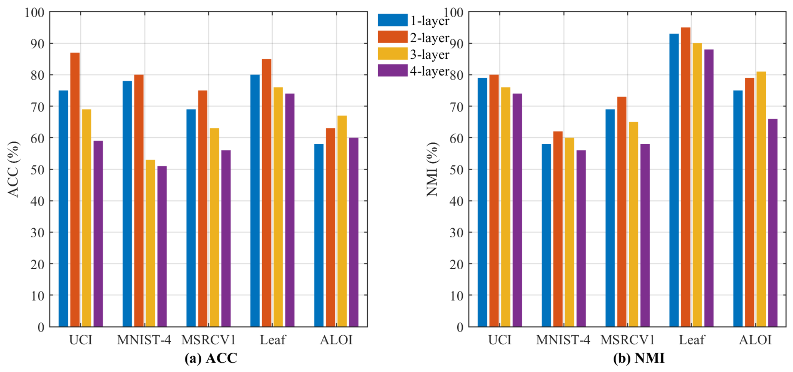
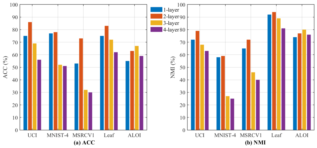
(1) Impact of Layer Numbers: To investigate the impact of different layer numbers adopted by the proposed method, we conducted numerical experiments on all five datasets by varying the number of layers, as shown in Figure 3 and Figure 4. Experiments were conducted by changing the number of layers m from 1 to 4, with corresponding layer sizes set to [50], [50, 100], [50, 100, 200], and [50, 100, 200, 300], respectively.

As illustrated in Figure 3 and Figure 4, multi-layer models consistently achieve better ACC and NMI scores than their single-layer counterparts across all datasets. This observation indicates that deep architectures are more capable of capturing hierarchical structures embedded in the data, thereby providing more expressive representations than shallow models. Moreover, the performance generally improves as the network depth increases, until an optimal depth is reached. Beyond this point, further increasing the number of layers leads to performance degradation, which can be attributed to overfitting. Consequently, selecting an appropriate model depth is crucial for different datasets. In our experiments, a two-layer GDNMF-MRL architecture is adopted for UCI, MSRCV1, MNIST-4, and Leaf, while a three-layer structure is employed for the ALOI dataset.

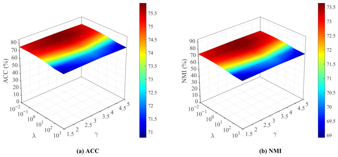
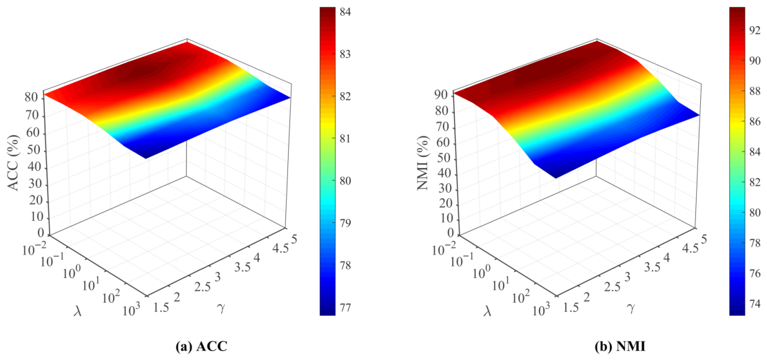
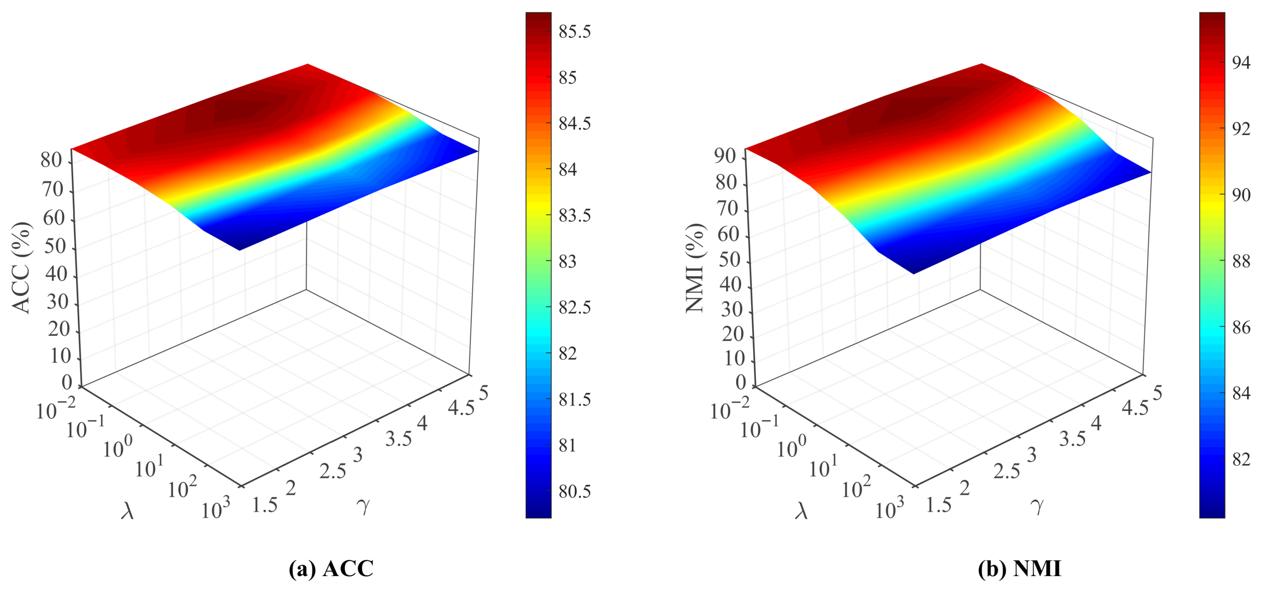
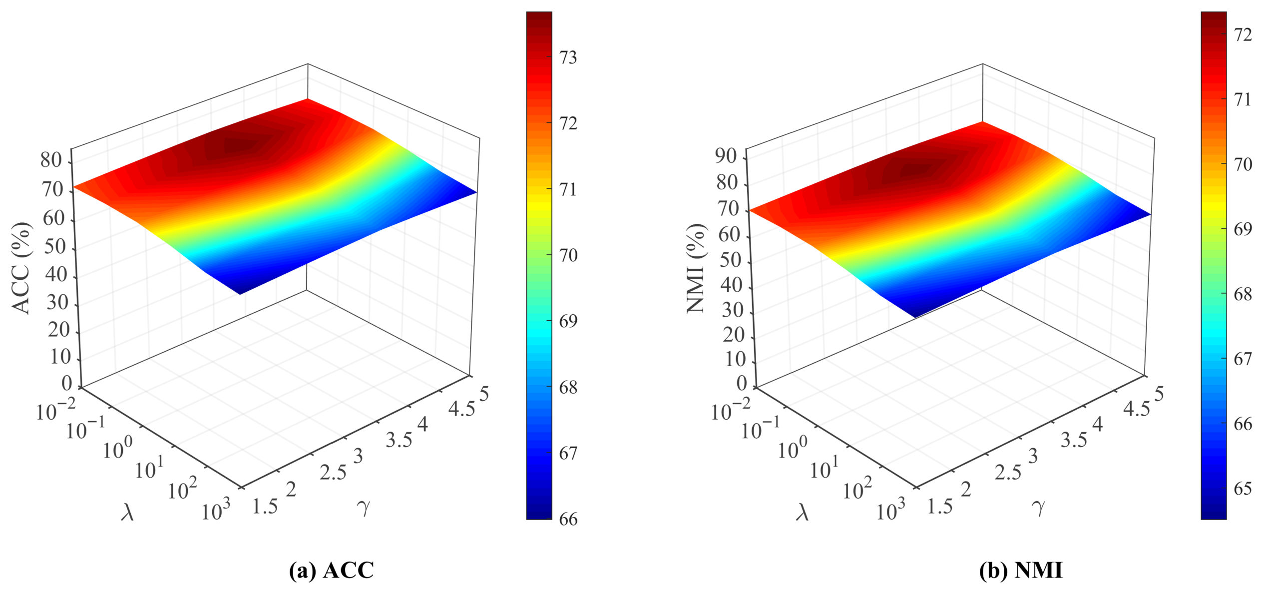
(2) Impact of Graph Regularization and Weight Distribution: To evaluate the impact of different components in the proposed model, we studied two important hyperparameters $\lambda$ and $\gamma$. Specifically, $\lambda$ and $\gamma$ control the contribution of graph regularization and the distribution of different views’ fusion weights $\alpha$, respectively. Based on the grid search strategy, $\lambda$ is selected from the range {0.01, 0.1, 1, 10, 100, 1000}, and $\gamma$ is selected from the range {1.5, 2, 2.5, 3, 3.5, 4, 4.5, 5}.

Figure 3. Clustering results of GDNMF-MRL with different numbers of layers on five datasets.

Figure 3. Clustering results of GDNMF-MRL with different numbers of layers on five datasets.

Figure 4. Clustering results of OS-GDNMF-MRL with different numbers of layers on five datasets.

Figure 4. Clustering results of OS-GDNMF-MRL with different numbers of layers on five datasets.

Taking the Leaf and MSRCV1 datasets as representative examples, as shown in Figure 5, Figure 6, Figure 7 and Figure 8, we can observe that both GDNMF-MRL and OS-GDNMF-MRL exhibit clear sensitivity to the graph regularization parameter $\lambda$, while showing relatively more stable behavior under varying $\gamma$ within a moderate range. On the Leaf dataset, GDNMF-MRL achieves its best performance when $\lambda =1.0$ and $\gamma =3.5$, reaching ACC of 83.5% and NMI of 93.91%. For OS-GDNMF-MRL, the best NMI performance (95.13%) is obtained when $\lambda$ is set to a small value and $\gamma =1.5$, while the ACC values remain robust across different parameter combinations. Similar trends can also be observed on the MSRCV1 dataset, where moderate $\lambda$ values consistently provide better clustering quality than excessively large ones. These observations suggest that both methods benefit from appropriate graph regularization strength, and that the overall parameter sensitivity patterns are relatively consistent across datasets with different characteristics.

5.6. Ablation and Convergence Study

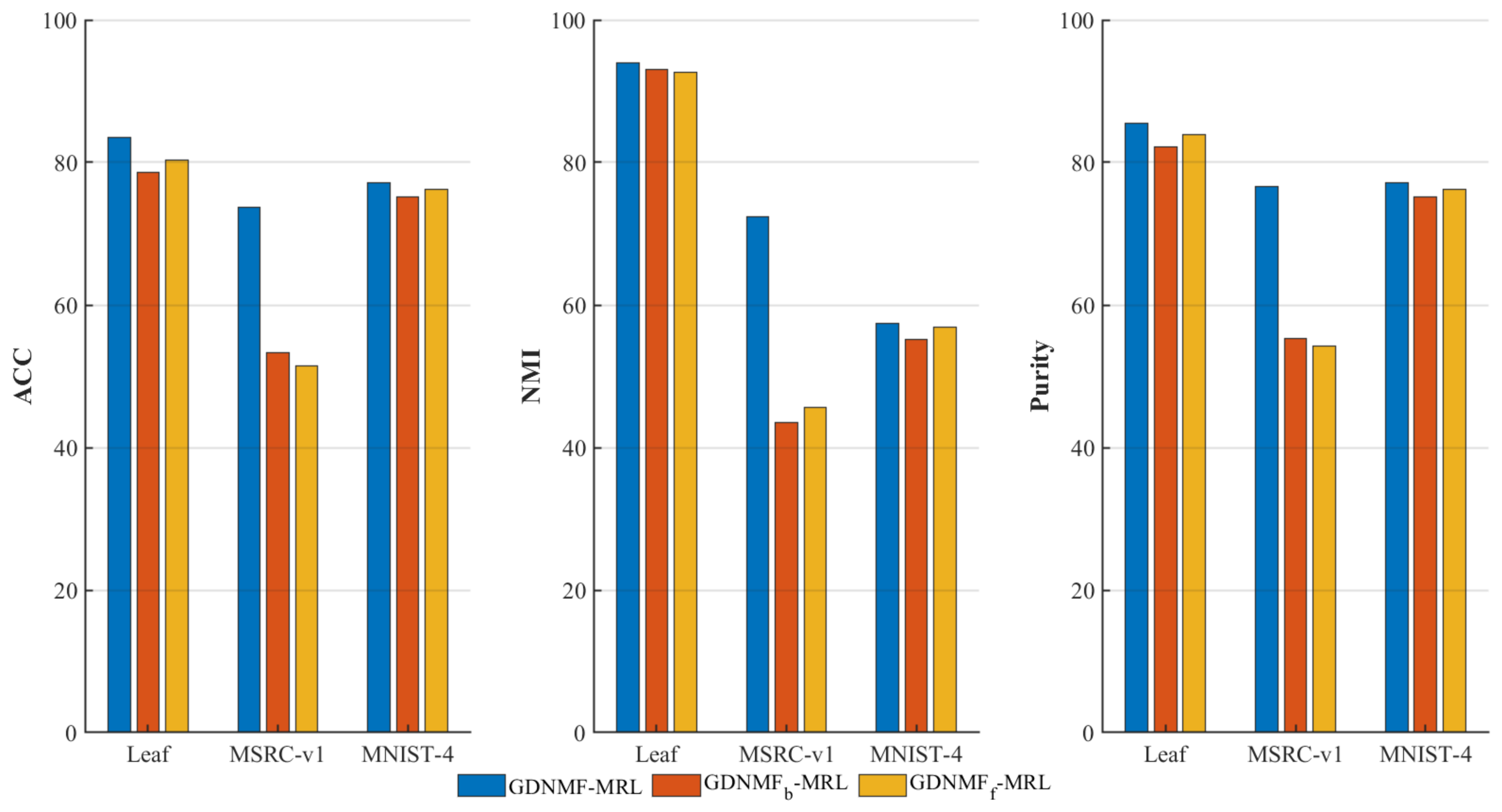
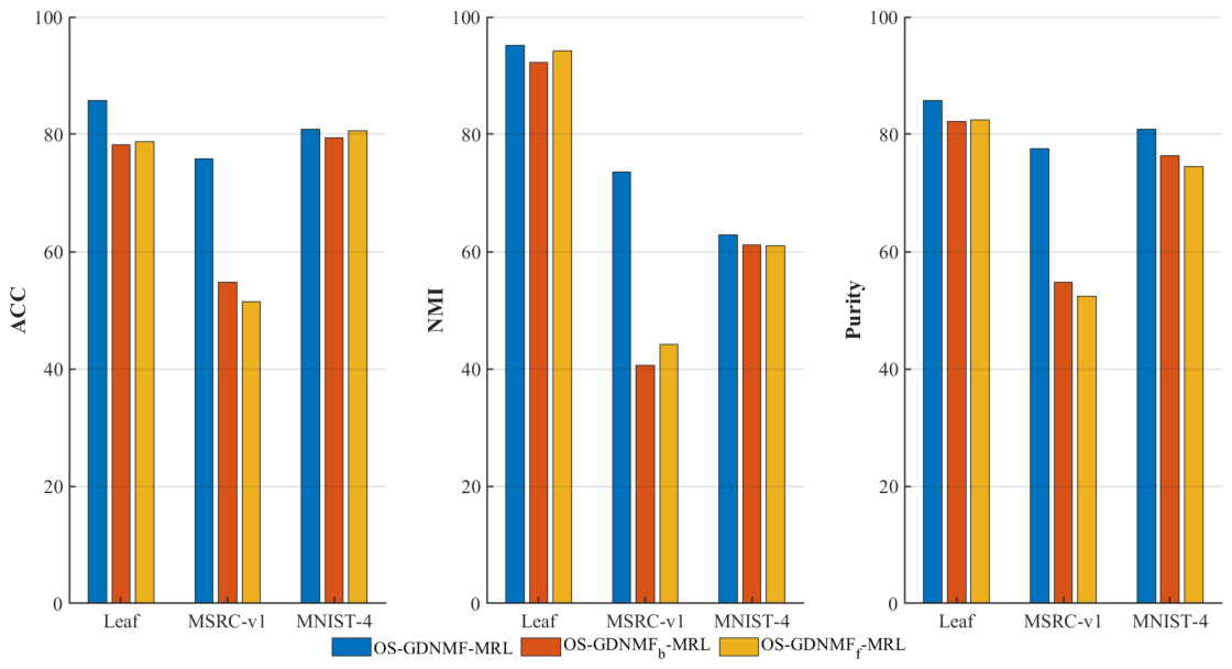
To investigate the effectiveness of deep decomposition on both features and bases in GDNMF-MRL, we conduct ablation studies by comparing the proposed model with two degraded variants: GDNMF-MRL with only basis decomposition (denoted as GDNMF_b) and GDNMF-MRL with only feature decomposition (denoted as GDNMF_f). Experiments are carried out on the Leaf, MSRCV1, and MNIST-4 datasets, and the corresponding results are presented in Figure 9. Similar trends are also observed on other datasets. For a fair comparison, all hyperparameters are kept identical across different variants. As shown in Figure 9, GDNMF-MRL consistently achieves better clustering performance than both GDNMF_b and GDNMF_f on all three datasets, which verifies that jointly performing deep decomposition on feature matrices and basis matrices leads to more expressive representations and improved clustering accuracy. In addition, analogous ablation experiments are conducted for OS-GDNMF-MRL, and similar conclusions are obtained, as illustrated in Figure 10.

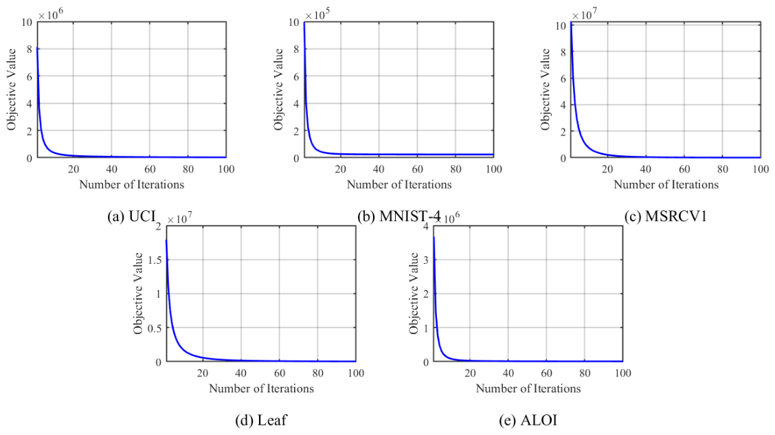
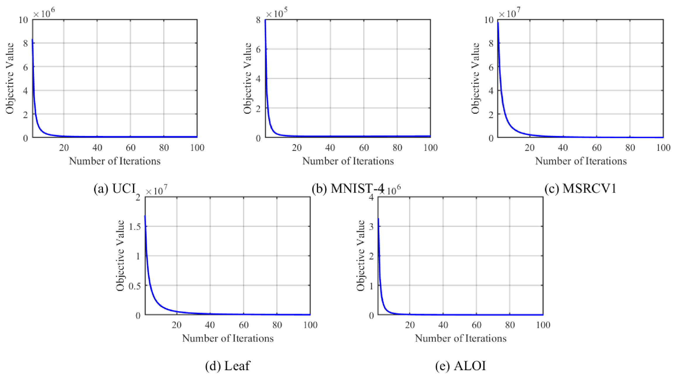
Furthermore, based on the update strategies described in the preceding optimization subsections, we empirically examine the convergence behavior of the proposed optimization algorithms. The convergence curves of GDNMF-MRL and OS-GDNMF-MRL are shown in Figure 11 and Figure 12, respectively, where the vertical axis denotes the objective function value and the horizontal axis represents the iteration number. It can be observed that both methods converge rapidly and typically stabilize within about 50 iterations. These results are consistent with the theoretical convergence analysis and demonstrate the efficiency and practicality of the proposed optimization schemes.

6. Conclusions

This paper presents a novel hierarchical multi-view representation learning framework, termed GDNMF-MRL, which extends generalized deep non-negative matrix factorization to the multi-view clustering setting. By jointly performing deep decomposition on both feature and basis matrices, the proposed model is capable of capturing multi-level hierarchical structures in multi-view data. Meanwhile, the integration of shallow linear and deep nonlinear components enables the model to preserve the favorable interpretability and robustness commonly associated with NMF-based methods.

Furthermore, a one-step variant, OS-GDNMF-MRL, is developed to unify representation learning and clustering assignment within a single optimization objective, thereby better exploiting latent cluster structures and avoiding the potential suboptimality of conventional two-stage approaches. Extensive experiments on multiple benchmark datasets demonstrate that the proposed methods consistently outperform several state-of-the-art shallow and deep multi-view clustering methods in terms of clustering accuracy, robustness, and stability.

Despite these encouraging results, several limitations of the proposed framework should be noted. First, the model involves multiple hyperparameters, including the graph regularization weight, the fusion-weight parameter, and the depth configuration, and its performance may be sensitive to their selection. Second, the effectiveness of the graph-regularized terms relies on the quality of the constructed affinity graphs, where inaccurate neighborhood relationships may adversely affect the learned representations. Third, the computational cost associated with graph construction and iterative deep matrix factorization may limit the scalability of the model when applied to very-large-scale datasets. In addition, similar to many deep factorization approaches, the optimization process may exhibit sensitivity to initialization and reduced stability when deeper architectures are adopted. These factors may also pose additional challenges in real-world applications, where large-scale data, noisy neighborhood relationships, and heterogeneous view quality are commonly encountered.

In future work, we will further investigate more scalable optimization strategies, adaptive hyperparameter selection mechanisms, robust graph learning approaches, and more stable deep factorization schemes.

References

1. Zhao, J.; Xie, X.; Xu, X.; Sun, S. Multi-view learning overview: Recent progress and new challenges. Inf. Fusion 2017, 38, 43–54. [Google Scholar] [CrossRef] [Scilit]
2. Xia, W.; Gao, Q.; Wang, Q.; Gao, X.; Ding, C.; Tao, D. Tensorized bipartite graph learning for multi-view clustering. IEEE Trans. Pattern Anal. Mach. Intell. 2023, 45, 5187–5202. [Google Scholar] [CrossRef] [Scilit] [PubMed]
3. Li, Y.; Yang, M.; Zhang, Z. A survey of multi-view representation learning. IEEE Trans. Knowl. Data Eng. 2019, 31, 1863–1883. [Google Scholar] [CrossRef] [Scilit]
4. Sun, K.; Zhang, J.; Liu, J.; Yu, R.; Song, Z. DRCNN: Dynamic routing convolutional neural network for multi-view 3D object recognition. IEEE Trans. Image Process. 2021, 30, 868–877. [Google Scholar] [CrossRef] [Scilit]
5. Zhang, X.; He, L.; Chen, K.; Luo, Y.; Zhou, J.; Wang, F. Multi-view graph convolutional network and its applications on neuroimage analysis for Parkinson’s disease. In AMIA Annual Symposium Proceedings; American Medical Informatics Association: Washington, DC, USA, 2018; p. 1147. [Google Scholar]
6. Xu, C.; Tao, D.; Xu, C. Multi-view intact space learning. IEEE Trans. Pattern Anal. Mach. Intell. 2015, 37, 2531–2544. [Google Scholar] [CrossRef] [Scilit]
7. Liu, X. Incomplete multiple kernel alignment maximization for clustering. IEEE Trans. Pattern Anal. Mach. Intell. 2021; early access.
8. Liu, J.; Liu, X.; Yang, Y.; Liao, Q.; Xia, Y. Contrastive multi-view kernel learning. IEEE Trans. Pattern Anal. Mach. Intell. 2023, 45, 9552–9566. [Google Scholar] [CrossRef] [Scilit] [PubMed]
9. Yu, J.; Zou, T.; Zhou, G. Online subspace learning and imputation by tensor-ring decomposition. Neural Netw. 2022, 153, 314–324. [Google Scholar] [CrossRef] [Scilit]
10. Vidal, R. Subspace clustering. IEEE Signal Process. Mag. 2011, 28, 52–68. [Google Scholar] [CrossRef] [Scilit]
11. Kang, Z.; Lu, X.; Yi, J.; Xu, Z. Self-weighted multiple kernel learning for graph-based clustering and semi-supervised classification. In Proceedings of the 27th International Joint Conference on Artificial Intelligence; AAAI Press: Stockholm, Sweden, 2018; pp. 2312–2318. [Google Scholar]
12. Yu, J.; Zhou, G.; Li, C.; Zhao, Q.; Xie, S. Low tensor-ring rank completion by parallel matrix factorization. IEEE Trans. Neural Netw. Learn. Syst. 2021, 32, 3020–3033. [Google Scholar] [CrossRef] [Scilit]
13. Wang, S.; Liu, X.; Zhu, X.; Zhang, P.; Zhang, Y.; Gao, F.; Zhu, E. Fast parameter-free multi-view subspace clustering with consensus anchor guidance. IEEE Trans. Image Process. 2022, 31, 556–568. [Google Scholar] [CrossRef] [Scilit]
14. Lee, D.D.; Seung, H.S. Algorithms for non-negative matrix factorization. In Proceedings of the 14th International Conference on Neural Information Processing Systems; MIT Press: Cambridge, MA, USA, 2000; pp. 535–541. [Google Scholar]
15. Ding, C.H.Q.; Li, T.; Jordan, M.I. Convex and semi-nonnegative matrix factorizations. IEEE Trans. Pattern Anal. Mach. Intell. 2008, 32, 45–55. [Google Scholar] [CrossRef] [Scilit]
16. Chen, W.-S.; Zeng, Q.; Pan, B. A survey of deep nonnegative matrix factorization. Neurocomputing 2022, 491, 305–320. [Google Scholar] [CrossRef] [Scilit]
17. Liu, H.; Wu, Z.; Li, X.; Cai, D.; Huang, T.S. Constrained nonnegative matrix factorization for image representation. IEEE Trans. Pattern Anal. Mach. Intell. 2011, 34, 1299–1311. [Google Scholar] [CrossRef] [Scilit]
18. Meng, Y.; Shang, R.; Shang, F.; Jiao, L.; Yang, S.; Stolkin, R. Semi-supervised graph regularized deep NMF with bi-orthogonal constraints for data representation. IEEE Trans. Neural Netw. Learn. Syst. 2019, 31, 3245–3258. [Google Scholar] [CrossRef] [Scilit]
19. Babaee, M.; Tsoukalas, S.; Babaee, M.; Rigoll, G.; Datcu, M. Discriminative nonnegative matrix factorization for dimensionality reduction. Neurocomputing 2016, 173, 212–223. [Google Scholar] [CrossRef] [Scilit]
20. Lan, L.; Guan, N.; Zhang, X.; Tao, D.; Luo, Z. Soft-constrained nonnegative matrix factorization via normalization. In 2014 International Joint Conference on Neural Networks (IJCNN); IEEE: Piscataway, NJ, USA, 2014; pp. 3025–3030. [Google Scholar]
21. Trigeorgis, G.; Bousmalis, K.; Zafeiriou, S.; Schuller, B.W. A deep matrix factorization method for learning attribute representations. IEEE Trans. Pattern Anal. Mach. Intell. 2016, 39, 417–429. [Google Scholar] [CrossRef] [Scilit] [PubMed]
22. Zhao, Y.; Wang, H.; Pei, J. Deep non-negative matrix factorization architecture based on underlying basis images learning. IEEE Trans. Pattern Anal. Mach. Intell. 2021, 43, 1897–1913. [Google Scholar] [CrossRef] [Scilit]
23. Yang, Z.; Li, Z.; Sun, L. Generalized discriminative deep non-negative matrix factorization based on latent feature and basis learning. In Proceedings of the 32nd International Joint Conference on Artificial Intelligenc, Macao, China, 19–25 August 2023; pp. 4486–4494. [Google Scholar]
24. Qiu, Y.; Zhou, G.; Wang, Y.; Zhang, Y.; Xie, S. A generalized graph regularized non-negative tucker decomposition framework for tensor data representation. IEEE Trans. Cybern. 2022, 52, 594–607. [Google Scholar] [CrossRef] [Scilit]
25. Zhang, S.; Li, X.; Zong, M.; Zhu, X.; Cheng, D. Learning k for kNN classification. ACM Trans. Intell. Syst. Technol. 2017, 8, 1–19. [Google Scholar] [CrossRef] [Scilit]
26. Yu, Y.; Zhou, G.; Huang, H.; Xie, S.; Zhao, Q. A semi-supervised label-driven auto-weighted strategy for multi-view data classification. Knowl.-Based Syst. 2022, 255, 109694. [Google Scholar] [CrossRef] [Scilit]
27. Zhang, S.; Li, X.; Zong, M.; Zhu, X.; Wang, R. Efficient kNN classification with different numbers of nearest neighbors. IEEE Trans. Neural Netw. Learn. Syst. 2018, 29, 1774–1785. [Google Scholar] [CrossRef] [Scilit]
28. Jiang, Z.; Liu, X. Adaptive KNN and graph-based autoweighted multi-view consensus spectral learning. Inf. Sci. 2022, 609, 1132–1146. [Google Scholar] [CrossRef] [Scilit]
29. Andrew, G.; Arora, R.; Bilmes, J.; Livescu, K. Deep canonical correlation analysis. In International Conference on Machine Learning; PMLR: New York, NY, USA, 2013; pp. 1247–1255. [Google Scholar]
30. Wang, C.; Chen, M.; Huang, L.; Cao, X.; Zhao, B. Smoothness regularized multiview subspace clustering with kernel learning. IEEE Trans. Neural Netw. Learn. Syst. 2021, 32, 5047–5060. [Google Scholar] [CrossRef] [Scilit] [PubMed]
31. Xie, Y.; Liu, J.; Qu, Y.; Tao, D.; Shen, H.T. Robust kernelized multiview self-representation for subspace clustering. IEEE Trans. Neural Netw. Learn. Syst. 2021, 32, 868–881. [Google Scholar] [CrossRef] [Scilit] [PubMed]
32. Zhang, C.; Fu, H.; Hu, Q.; Cao, X.; Xie, Y.; Tao, D.; Xu, D. Generalized latent multi-view subspace clustering. IEEE Trans. Pattern Anal. Mach. Intell. 2020, 42, 86–99. [Google Scholar] [CrossRef] [Scilit]
33. Xiao, X.; Chen, Y.; Gong, Y.; Zhou, Y. Prior knowledge regularized multiview self-representation and its applications. IEEE Trans. Neural Netw. Learn. Syst. 2021, 32, 1325–1338. [Google Scholar] [CrossRef] [Scilit]
34. Zhu, X.; Zhang, S.; He, W.; Hu, R.; Lei, C.; Zhu, P. One-step multiview spectral clustering. IEEE Trans. Knowl. Data Eng. 2019, 31, 2022–2034. [Google Scholar] [CrossRef] [Scilit]
35. Wang, H.; Yang, Y.; Liu, B. GMC: Graph-based multi-view clustering. IEEE Trans. Knowl. Data Eng. 2020, 32, 1116–1129. [Google Scholar] [CrossRef] [Scilit]
36. Wang, W.; Arora, R.; Livescu, K.; Bilmes, J. On deep multi-view representation learning. In International Conference on Machine Learning; PMLR: New York, NY, USA, 2015; pp. 1083–1092. [Google Scholar]
37. Xu, J.; Ren, Y.; Tang, H.; Yang, Z.; Pan, L.; Yang, Y.; Pu, X. Multi-VAE: Learning disentangled view-common and view-peculiar visual representations for multi-view clustering. In Proceedings of the IEEE/CVF International Conference on Computer Vision; IEEE: Piscataway, NJ, USA, 2021; pp. 9214–9223. [Google Scholar]
38. Zhang, C.; Geng, Y.; Han, Z.; Liu, Y.; Fu, Z.; Hu, Q. Autoencoder in autoencoder networks. IEEE Trans. Neural Netw. Learn. Syst. 2022, 35, 2263–2275. [Google Scholar] [CrossRef] [Scilit]
39. Yang, M.; Li, Y.; Hu, P.; Bai, J.; Lv, J.C.; Pei, M. Robust multiview clustering with incomplete information. IEEE Trans. Pattern Anal. Mach. Intell. 2023, 45, 1055–1069. [Google Scholar] [CrossRef] [Scilit]
40. Ding, C.; Li, T.; Peng, W.; Park, H. Orthogonal nonnegative matrix t-factorizations for clustering. In Proceedings of the 12th ACM SIGKDD International Conference on Knowledge Discovery and Data Mining; Association for Computing Machinery: New York, NY, USA, 2006; pp. 126–135. [Google Scholar]
41. Liu, J.; Wang, C.; Gao, J.; Han, J. Multi-view clustering via joint nonnegative matrix factorization. In Proceedings of the 2013 SIAM International Conference on Data Mining; Society for Industrial and Applied Mathematics: Philadelphia, PA, USA, 2013; pp. 252–260. [Google Scholar]
42. Wang, J.; Tian, F.; Yu, H.; Liu, C.H.; Zhan, K.; Wang, X. Diverse non-negative matrix factorization for multiview data representation. IEEE Trans. Cybern. 2018, 48, 2620–2632. [Google Scholar] [CrossRef] [Scilit]
43. Liang, N.; Yang, Z.; Li, Z.; Xie, S.; Su, C. Multi-view clustering by non-negative matrix factorization with co-orthogonal constraints. Knowl.-Based Syst. 2020, 194, 105582. [Google Scholar] [CrossRef] [Scilit]
44. Cao, X.; Zhang, C.; Fu, H.; Liu, S.; Zhang, H. Diversity-induced multi-view subspace clustering. In Proceedings of the IEEE/CVF Conference on Computer Vision and Pattern Recognition; IEEE: Piscataway, NJ, USA, 2015; pp. 586–594. [Google Scholar]
45. Wang, H.; Yang, Y.; Li, T. Multi-view clustering via concept factorization with local manifold regularization. In 2016 IEEE 16th International Conference on Data Mining (ICDM); IEEE: Piscataway, NJ, USA, 2016; pp. 1245–1250. [Google Scholar]
46. Zong, L.; Zhang, X.; Zhao, L.; Yu, H.; Zhao, Q. Multi-view clustering via multi-manifold regularized non-negative matrix factorization. Neural Netw. 2017, 88, 74–89. [Google Scholar] [CrossRef] [Scilit]
47. Yang, Z.; Liang, N.; Yan, W.; Li, Z.; Xie, S. Uniform distribution non-negative matrix factorization for multiview clustering. IEEE Trans. Cybern. 2021, 51, 3249–3262. [Google Scholar] [CrossRef] [Scilit] [PubMed]
48. Peng, S.; Yin, J.; Yang, Z.; Liu, Y.; Wang, J. Multiview clustering via hypergraph induced semi-supervised symmetric nonnegative matrix factorization. IEEE Trans. Circuits Syst. Video Technol. 2023, 33, 5510–5524. [Google Scholar] [CrossRef] [Scilit]
49. Deng, P.; Li, T.; Wang, D.; Wang, H.; Zhang, H. Multi-view clustering guided by unconstrained non-negative matrix factorization. Knowl.-Based Syst. 2023, 266, 110425. [Google Scholar] [CrossRef] [Scilit]
50. Li, C.; Che, H.; Leung, M.-F.; Liu, T. Robust multi-view non-negative matrix factorization with adaptive graph and diversity constraints. Inf. Sci. 2023, 634, 587–607. [Google Scholar] [CrossRef] [Scilit]
51. Liu, H.; Yu, X.; Lin, Y.; Chen, B.; Wang, L. Similarity-induced weighted consensus Laplacian matrix learning for multiview clustering. IEEE Trans. Syst. Man Cybern. Syst. 2024, 54, 6113–6126. [Google Scholar] [CrossRef] [Scilit]
52. Huang, H.; Liang, N.; Yan, W.; Wang, X.; Zhou, G. Partially shared semi-supervised deep matrix factorization with multi-view data. In 2020 International Conference on Data Mining Workshops (ICDMW); IEEE: Piscataway, NJ, USA, 2020; pp. 564–570. [Google Scholar]
53. Huang, H.; Zhou, G.; Liang, N.; Yang, Z.; Xie, S. Diverse deep matrix factorization with hypergraph regularization for multiview data representation. IEEE/CAA J. Autom. Sin. 2023, 10, 2154–2167. [Google Scholar] [CrossRef] [Scilit]
54. Huang, H.; Zhou, G.; Zheng, Y.; Yang, Z.; Zhao, Q. Exclusivity and consistency induced NMF for multi-view representation learning. Knowl.-Based Syst. 2023, 281, 111020. [Google Scholar] [CrossRef] [Scilit]
55. Luong, K.; Nayak, R. A Novel Approach to Learning Consensus and Complementary Information for Multi-View Data Clustering. In Proceedings of the 2020 IEEE 36th International Conference on Data Engineering (ICDE), Dallas, TX, USA, 20–24 April 2020; IEEE: Piscataway, NJ, USA, 2020; pp. 865–876. [Google Scholar]
56. Xiang, S.J.; Li, H.C.; Yang, J.H.; Feng, X.R. Dual Auto-Weighted Multi-View Clustering via Autoencoder-like Nonnegative Matrix Factorization. Inf. Sci. 2024, 667, 120458. [Google Scholar] [CrossRef] [Scilit]
57. Zhao, H.; Ding, Z.; Fu, Y. Multi-View Clustering via Deep Matrix Factorization. In Proceedings of the Thirty-First AAAI Conference on Artificial Intelligence, San Francisco, CA, USA, 4–9 February 2017; Singh, S., Markovitch, S., Eds.; AAAI Press: Washington, DC, USA, 2017; pp. 2921–2927. [Google Scholar]
58. Zhong, B.; Wu, J.-Y.; Wu, J.-S.; Min, W. Multi-view deep reciprocal nonnegative matrix factorization. Eng. Appl. Artif. Intell. 2025, 139, 109508. [Google Scholar]
59. Fu, L.; Chen, Z.; Chen, Y.; Wang, S. Unified low-rank tensor learning and spectral embedding for multi-view subspace clustering. IEEE Trans. Multimed. 2022; early access.
Figure 1. Illustration of GDNMF reconstruction using deep nonlinear and shallow linear components. Taking the two-layer case as an example, Deep FBD simultaneously conducts hierarchical decomposition on the feature component G 1 and the basis component F 1 .
Mathematics 14 01442 g001
Figure 2. Overview of the proposed GDNMF-MRL model.
Mathematics 14 01442 g002
Figure 5. ACC and NMI versus parameters λ and γ of GDNMF-MRL on the Leaf dataset.
Mathematics 14 01442 g005
Figure 6. ACC and NMI versus parameters λ and γ of OS-GDNMF-MRL on the Leaf dataset.
Mathematics 14 01442 g006
Figure 7. ACC and NMI versus parameters λ and γ of GDNMF-MRL on the MSRCV1 dataset.
Mathematics 14 01442 g007
Figure 8. ACC and NMI versus parameters λ and γ of OS-GDNMF-MRL on the MSRCV1 dataset.
Mathematics 14 01442 g008
Figure 9. Ablation study of GDNMF-MRL on the Leaf, MSRCV1, and MNIST-4 datasets in terms of ACC, NMI, and Purity. The degraded variants only consider basis decomposition and feature decomposition, respectively.
Mathematics 14 01442 g009
Figure 10. Ablation study of OS-GDNMF-MRL on the Leaf, MSRCV1, and MNIST-4 datasets in terms of ACC, NMI, and Purity. The degraded variants only consider basis decomposition and feature decomposition, respectively.
Mathematics 14 01442 g010
Figure 11. Convergence curves of GDNMF-MRL on five benchmark datasets. From left to right and top to bottom, the five panels correspond to UCI, MNIST-4, MSRCV1, Leaf, and ALOI, respectively.
Mathematics 14 01442 g011
Figure 12. Convergence curves of OS-GDNMF-MRL on five benchmark datasets. From left to right and top to bottom, the five panels correspond to UCI, MNIST-4, MSRCV1, Leaf, and ALOI, respectively.
Mathematics 14 01442 g012