Article

Multi-Objective Trajectory Optimization Method for Connected Autonomous Vehicles Based on Risk Potential Field

1
School of Mechanical and Automotive Engineering, Qingdao University of Technology, Qingdao 266525, China
2
Intelligent Manufacturing Institute, Qingdao Huanghai University, Qingdao 266427, China
3
School of Civil Engineering, Qingdao University of Technology, Qingdao 266525, China
*
Authors to whom correspondence should be addressed.
Mathematics 2026, 14(9), 1415; https://doi.org/10.3390/math14091415
Submission received: 24 March 2026 / Revised: 16 April 2026 / Accepted: 20 April 2026 / Published: 23 April 2026
(This article belongs to the Special Issue Advanced Methods in Intelligent Transportation Systems, 2nd Edition)

Abstract

The planning of trajectories for Connected Autonomous Vehicles (CAVs) represents a pivotal aspect of autonomous driving technologies, enabling secure navigation within traffic environments. Traditional models for trajectory control primarily focus on the efficiency and safety of individual vehicles but often overlook the dynamics involved in vehicle-to-vehicle and vehicle-to-infrastructure interactions. This study introduces a novel concept, the “driving risk field,” which imposes constraints on vehicular movement within designated road spaces to enhance safety. A vehicle dynamics model is developed, employing a non-linear fifth-degree polynomial to approximate the trajectory curves, with optimization performed using the Sequential Quadratic Programming (SQP) method. The efficacy of the optimized model is validated through simulations on the Prescan/Simulink platform, demonstrating a 17.9% reduction in trajectory angle slopes and a 23.4% decrease in lateral and longitudinal errors compared to conventional Model Predictive Control (MPC), Pure-Pursuit (PP) and Linear Quadratic Regulator (LQR) models. This approach significantly enhances vehicle control in traffic bottleneck areas, indicating superior trajectory adaptation.

1. Introduction

Trajectory planning control for autonomous vehicles is a critical challenge in current autonomous driving technology. Specifically, the goal of trajectory planning is to model road spatial constraints and vehicle dynamic constraints based on real-time analysis of the vehicle’s surrounding environment and its own motion state within complex traffic conditions. Prioritizing safety while balancing passenger comfort, trajectory smoothness, and traffic flow efficiency, this process generates the optimal driving path. Traditional trajectory planning methods primarily fall into four categories: graph-based search approaches [1], sampling-based methods [2], curve-based techniques [3], and numerical optimization methods [4,5].
With advancements in computer hardware performance and artificial neural network technology, the current frontier of trajectory planning research is shifting toward learning-based methods and game theory-based approaches. Borkar et al. [6] proposed a generative adversarial network-based trajectory planning algorithm that directly generates optimal paths using multimodal perception data as input. Piri [7] et al. compared the interaction behaviors of human drivers with two types of vehicles equipped with advanced driver assistance systems (ADAS) across different road types based on naturalistic driving study data. The results also indicated that human drivers exhibited overall safer driving behavior when following readily identifiable vehicles. This study emphasizes that the visibility of appearance features of autonomous vehicles should be fully considered in traffic management and vehicle design to optimize traffic flow and improve road safety. Rahmanidehkordi [8] et al. proposed a traffic management algorithm applicable to heterogeneous freeway corridors consisting of human-driven vehicles (HVs) and autonomous vehicles (AVs). The algorithm is modeled using the heterogeneous METANET model and adopts variable speed control to maintain desired vehicle densities. By associating constraints on virtual control inputs with actual control commands, it effectively improves road traffic efficiency. Yang et al. [9] introduced a novel deep reinforcement learning trajectory planning algorithm, DRL-PP, which identifies optimal action sequences from the vehicle’s initial position to the destination to derive optimal trajectories. Despite their advantages, current learning-based methods still face multiple challenges [10,11]. This approach relies heavily on large-scale, high-quality datasets to learn complex mappings between features and trajectories, creating strong dependency on such datasets. Current datasets are often limited to single scenarios (e.g., highways), resulting in trajectory planning strategies with insufficient generalization capabilities and inability to handle unexpected events. The black-box nature of algorithms leads to poor interpretability in learning-based methods, obscuring the underlying logic of vehicle trajectory optimization and posing risks to driving safety. Yan et al. [12] developed a game-theoretic framework for mixed-traffic trajectory planning. Utilizing Stackelberg games and cooperative game methods, they solved the interactive games among lead vehicles, human-driven vehicles (HVs), and autonomous vehicles (AVs) across various AH-HV mixed driving environments. Game-theoretic approaches account for dynamic interactions among multiple agents and balance multiple optimization objectives. However, these methods currently face significant challenges [13,14]: In complex real-world multi-vehicle scenarios, the number of possible game states and strategy combinations grows exponentially, leading to prohibitively high computational complexity that cannot meet real-time planning requirements. Current game modeling assumes rational agents, yet real-world driver and pedestrian behaviors exhibit high uncertainty and irrationality, making perfect alignment with theoretical models challenging. Game equilibrium solutions may not be unique, and stable solutions may even be nonexistent in complex interaction scenarios; existing game models predominantly focus on decision interactions and profit maximization, neglecting trajectory comfort and smoothness requirements.
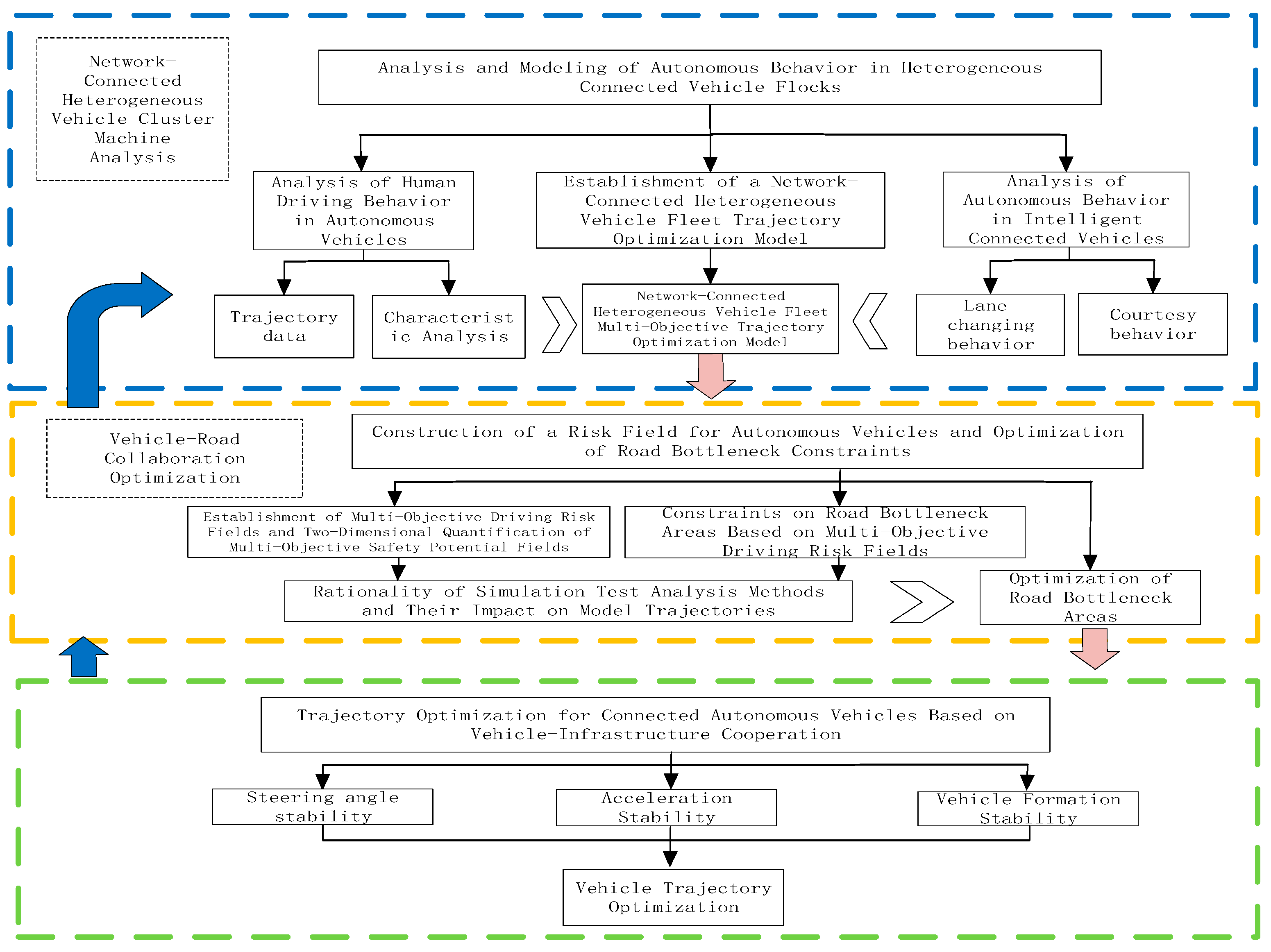
The concept of artificial potential fields originated from path planning research in robotics at the end of the 20th century. As traffic systems become increasingly intelligent, artificial potential fields have gradually been applied to transportation scenarios. In traffic systems, a vehicle’s behavior of neither getting too close to nor straying too far from the vehicle ahead can be viewed as the vehicle being influenced by field forces. Under the action of these forces, the vehicle continuously accelerates and decelerates in pursuit of equilibrium with the preceding vehicle. Within the traffic environment, each participant can be regarded as a field source, exerting forces on other sources. Inspired by this, researchers worldwide have extended artificial potential field concepts to autonomous vehicle motion planning. Qu Dayi et al. [15] constructed a Lennard-Jones potential field and proposed a vehicle following model based on this potential. Meng Yiming et al. [16] proposed a vehicle following behavior model based on molecular force fields; Wang Bo et al. [17] introduced a method for identifying highway driving risks based on a velocity risk potential field. Jia Yanfeng et al. [18] addressed the flaw of separating gravitational and repulsive forces in safety potential fields; Li Linhenget al. [19] developed a driving risk potential field based on acceleration and steering angle; Liu Peng et al. [20] conducted research on structured road obstacle safety potential fields; and Wang Jianqiang et al. [21] and Lu Shaobo et al. [22] focused on pedestrian crossing safety potential fields, quantifying pedestrian crossing risks. A. Li [23] et al. investigated the trajectory planning problem for obstacle avoidance of autonomous vehicles on structured roads and proposed a decoupled planning method for path and speed. They improved the obstacle repulsive potential field, gravitational potential field, and fitting approach in the traditional artificial potential field (APF), thereby significantly enhancing the driving safety and ride comfort of the vehicle. The introduction of artificial potential fields has largely resolved the challenge of quantifying vehicle risks, making risks during vehicle operation tangible and data-driven, thereby advancing autonomous driving technology. This paper proposes a driving risk field that accounts for phase-field coupling effects from multiple risk sources. The overall driving risk field incorporates various traffic elements (vehicles, pedestrians, static obstacles, lane lines, and lane boundaries). By superimposing these multi-source risk fields, it reflects the field-effect coupling between different risk factors. The vehicle risk field employs molecular mechanics modeling to quantify complex dynamic nonlinear interactions between vehicles. The pedestrian risk field utilizes an asymmetric dynamic field structure. Additionally, risk potential fields for lane lines and road boundaries are designed, implementing spatial constraints in road bottleneck zones that account for vehicle-vehicle, vehicle-road, and human-vehicle interactions. The vehicle risk field is further coupled with a vehicle dynamics model to generate trajectories that prioritize stability, safety, and comfort. Finally, trajectories are optimized through nonlinear polynomial fitting and solved using the SQP (Sequential Quadratic Programming) algorithm. The technical approach is shown in Figure 1:

2. Risk-Constrained Optimization in Traffic Bottleneck Areas

2.1. Construction of a Driving Risk Field

In the realm of physics, the term “field” denotes a region characterized by the interactions between objects and the transmission of energy, conceptualized as a continuous distribution of numerous particles. Each particle within this distribution is subject to the forces exerted by the field. Fields are categorized into two types: scalar fields, which represent a single physical quantity, and vector fields, which encompass multiple physical quantities such as force, speed, direction, and field intensity. Potential energy, defined as the energy stored within a system or field, is not confined to a single object but is distributed among interacting entities. The integration of a field with its potential energy results in what is known as a potential field. This field comprises both an attractive field, induced by a target point Uattr(q), and a repulsive field, caused by obstacles Urep(q). Therefore, a potential field effectively encapsulates the interactive forces within the space surrounding an object. In traffic systems, the concept of a potential field is particularly applicable. Here, each vehicle may be considered an individual particle within the field. The behavior of vehicles, influenced by surrounding vehicles to maintain optimal spacing and avoid collisions, parallels the dynamics observed in physical fields. For example, a proton is influenced by both attractive and repulsive forces as it seeks an optimal equilibrium. Within the context of an intelligent networked environment, driver-assistance decision systems play a crucial role. With the proliferation of CAVs (Connected Autonomous Vehicles), these otherwise invisible interacting forces are visualized and rendered comprehensible to human drivers. Each factor impacting a vehicle is considered a source within the field. The development of a multi-objective driving risk field integrates various risk potential fields, quantifying the interactions among them. This integration, in conjunction with the behavioral patterns of traffic entities, aids in the generation of safe and effective vehicle behavior decisions.
CAVs are required to interact not only with surrounding vehicles but also with road boundaries, pedestrians, various signs, and road obstacles. Consequently, a comprehensive driving risk field is constructed. This field includes vehicle risk potential fields, road boundary risk potential fields, road lane potential fields, asymmetric pedestrian potential fields, and road obstacle risk potential fields. The operation of CAVs within this field can be perceived as the result of the superposition of interactions among these various risk potential fields. As illustrated in Table 1, a Cartesian coordinate system is utilized to analyze these potential fields in two dimensions.

2.1.1. Vehicle Risk Potential Field

The vehicle risk potential field emerges from the interactive forces between vehicles. Drawing upon the principles of the Lennard-Jones potential, a unified vehicle potential field function has been developed. This function integrates considerations of the vehicle’s requisite risk distance and its following behavior. Thus, the vehicle risk potential field model is articulated as follows:
ψ c = ε p q q X r L p p X r L q · exp cos ν d · d d X L = β v + α v 2 + 0 T 0 λ [ a ( τ ) a p ( τ ) ] d τ d λ + 0 T [ v ( 0 ) v p ( 0 ) ] d t
where
ψ c symbolizes the vehicle risk potential field;
ε represents the magnitude of potential field energy;
p is the exponent governing the repulsive component;
q designates the exponent for the attractive component;
X r specifies the risk distance required by the vehicle;
L represents the actual vehicle spacing;
d is a coefficient that modifies the extent of the short-range repulsive potential field;
ν is the angle measured clockwise between any arbitrary point around the vehicle and the vehicle’s centroid;
v , v p are the speed of the following vehicle relative to the preceding vehicle;
a , a p are the acceleration of the following vehicle relative to the preceding vehicle;
β is the vehicle reaction time, take 1 s.;
α is the reciprocal of the square of the maximum deceleration for the vehicle is 0.07 m/s2;
T is the time to frontal collision between the vehicle and the preceding vehicle.

2.1.2. Lane Line Risk Potential Field

Within the framework of road traffic environments, lane markings typically fall into two categories: those delineating lanes for vehicles traveling in the same direction and those for vehicles traveling in opposite directions. The boundary line of the road serves as the y-axis origin, and a Gaussian-like function characterizes the potential field induced by lane markings, as depicted in the following:
ψ r = i = 1 N 1 P n · exp y y i 2 2 σ 2 · y y i y y i
where
N is the total number of lane markings present across a given road segment;
y is the y-coordinate of any given point;
P n is the potential field strength coefficient for different lane markings;
n indicates the type of lane marking, with n = 1 for white dashed lines and n = 2 for double yellow lines;
y i is the y-coordinate of the i -th lane marking;
σ is proportional to the road’s width, and reflects the rate at which the strength of the potential field diminishes at the road boundaries.
The risk potential field generated at the road’s boundary originates at the edge of the roadway. Its strength increases indefinitely as the distance from the vehicle extends. Contrasting with the vehicle risk potential field, the road boundary risk potential field is relatively static in location and demonstrates a significantly rapid and nonlinear enhancement in field strength as the proximity between the vehicle and the boundary reduces. Furthermore, the repulsive force exerted by the road boundary risk potential field on a vehicle considerably outweighs its attractive force. The refined repulsive function for the road boundary potential field is delineated in the following:
ψ l = a = 1 2 1 2 δ 1 d a y 2 · d a y d a y
d a y = y a y l
where
a designates the road boundaries, with a = 1 as the right boundary and a = 2 as the left boundary of the road;
d a y is the vertical coordinate difference between the vehicle at point y and the road boundary at the same point;
y a is the y-coordinate of the vehicle’s centroid;
y l is the y-coordinate of the road boundary;
δ is a positional gain function.
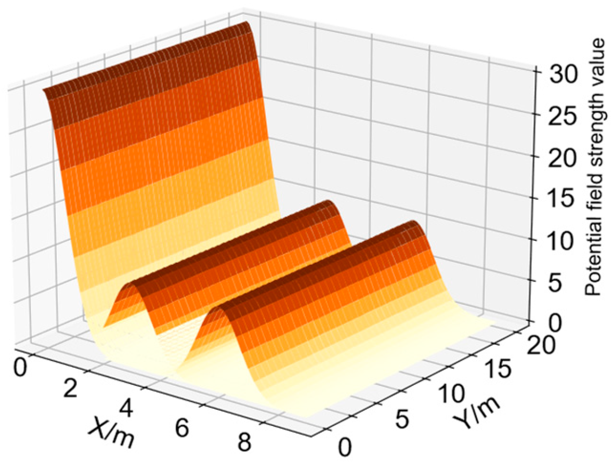
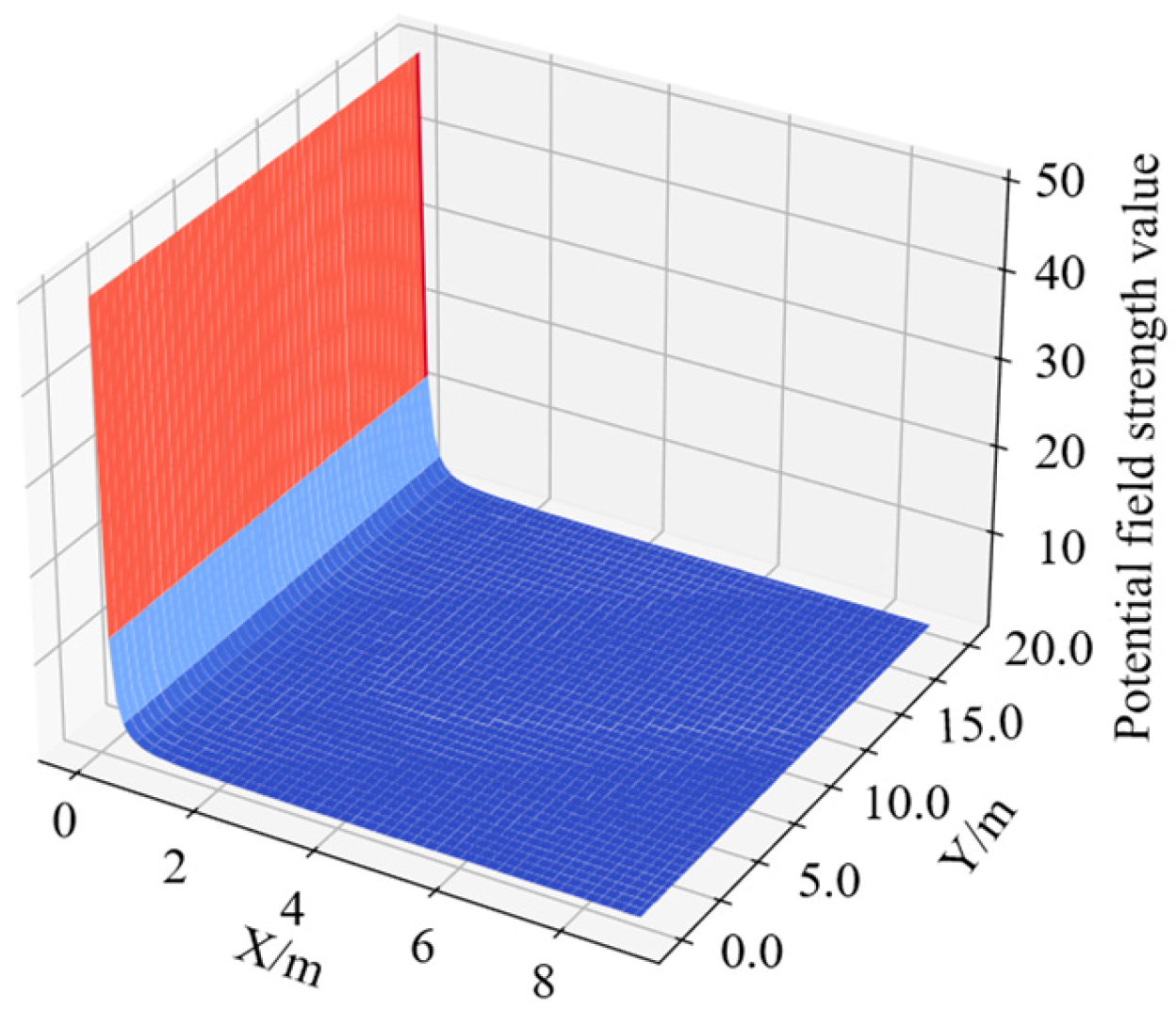
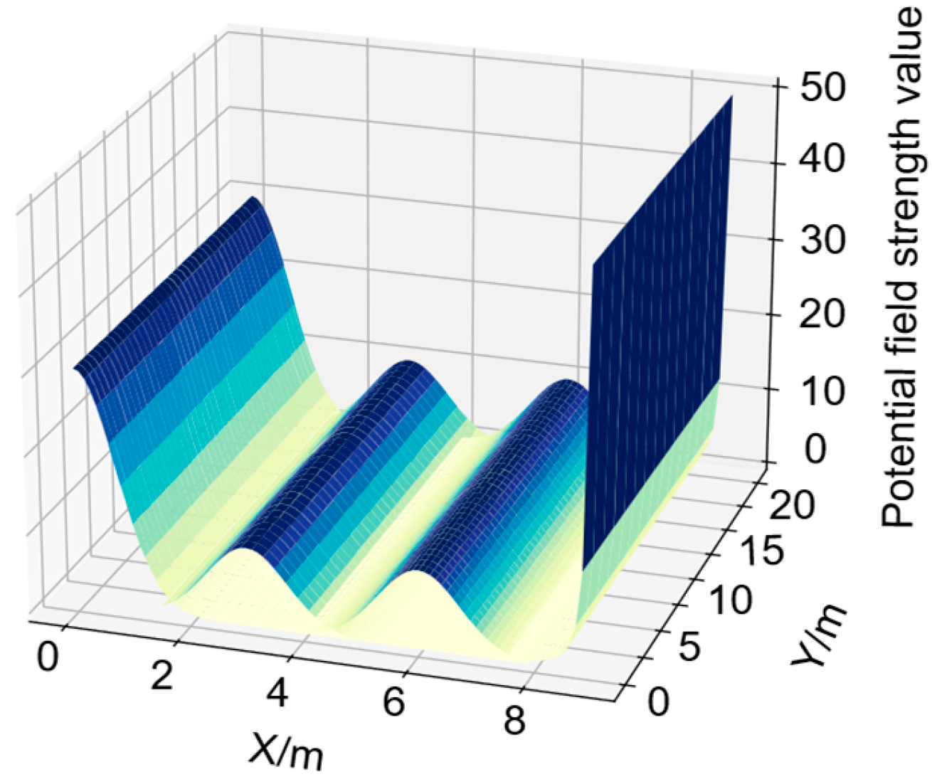
The integration of the lane risk potential field and the road boundary risk potential field is illustrated in Figure 2 for the lane risk potential field, Figure 3 for the road boundary risk potential field, and Figure 4 for the combined potential field subsequent to the overlay.
As depicted in Figure 4, the potential field intensity at the road boundary surpasses that adjacent to the double yellow line and is considerably higher than that near the white dashed line. The combined potential field strength reaches its peak at the road boundary and diminishes to its minimum at the road’s midpoint.

2.1.3. Static Obstacle Risk Potential Field

The risk potential field associated with static obstacles on roadways is determined by the presence of such obstructions and the inherent environmental factors of the road. This field emanates from the obstacles, viewed as discrete entities, and radiates outward, thereby establishing a surrounding risk potential field. This concept is expressed in the following:
ψ * = P * exp 1 2 x v x * λ 1 * ε 1 + y v y * λ 2 * ε 2
In this equation:
ψ * signifies the intensity of the risk potential field as influenced by road factors.
P * denotes the coefficient reflecting the impact of road influence factors on the risk potential field.
x v , y v are the longitudinal and lateral coordinates of the vehicle’s center of mass, respectively.
x * , y * are the longitudinal and lateral coordinates of the center of mass for the road influence factors.
ε 1 , ε 2 , λ 1 * , λ 2 * are the shape coefficients of the risk potential field, with λ 1 * , λ 2 * primarily determined by the geometric dimensions of the influence factors.
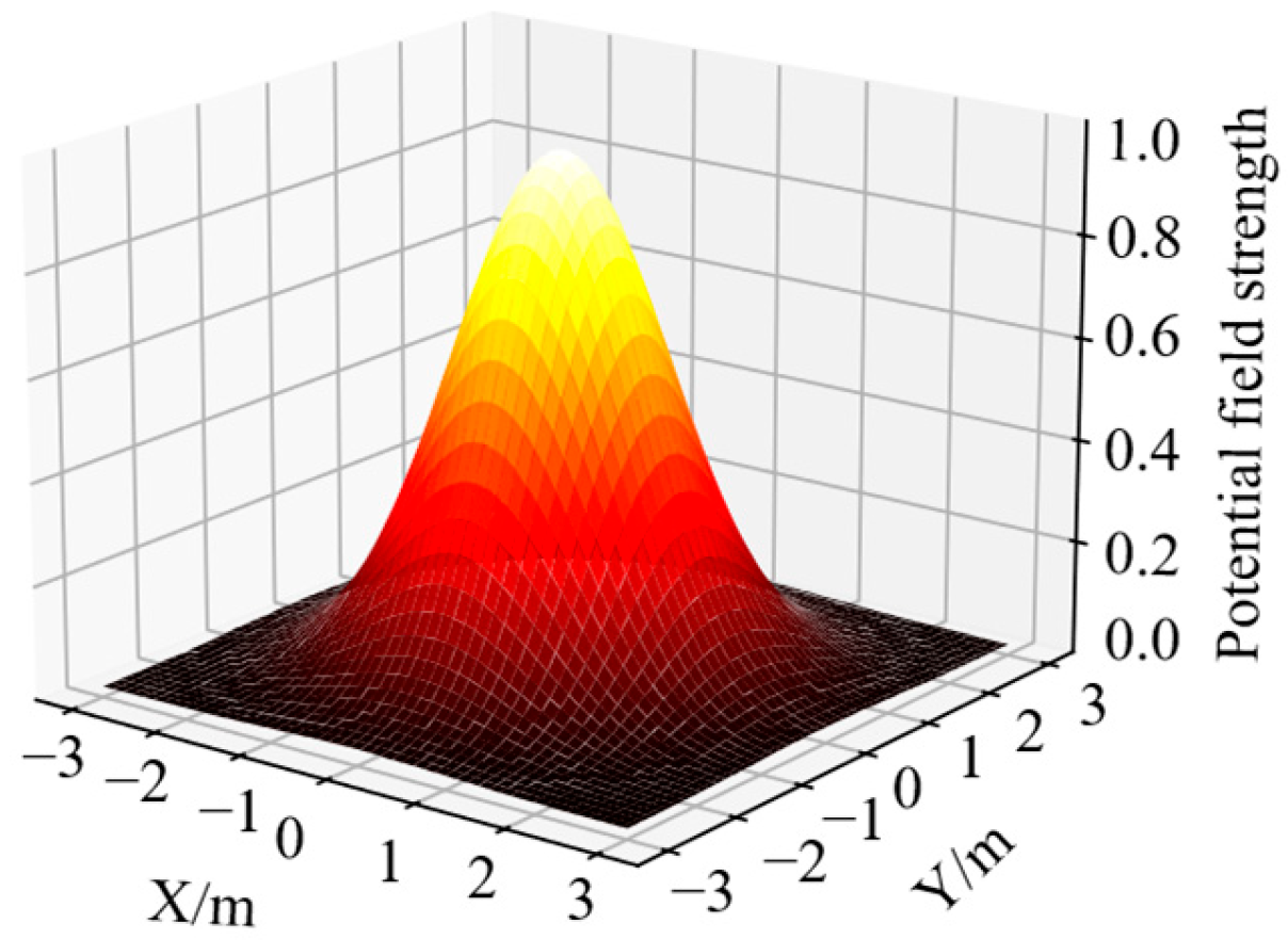
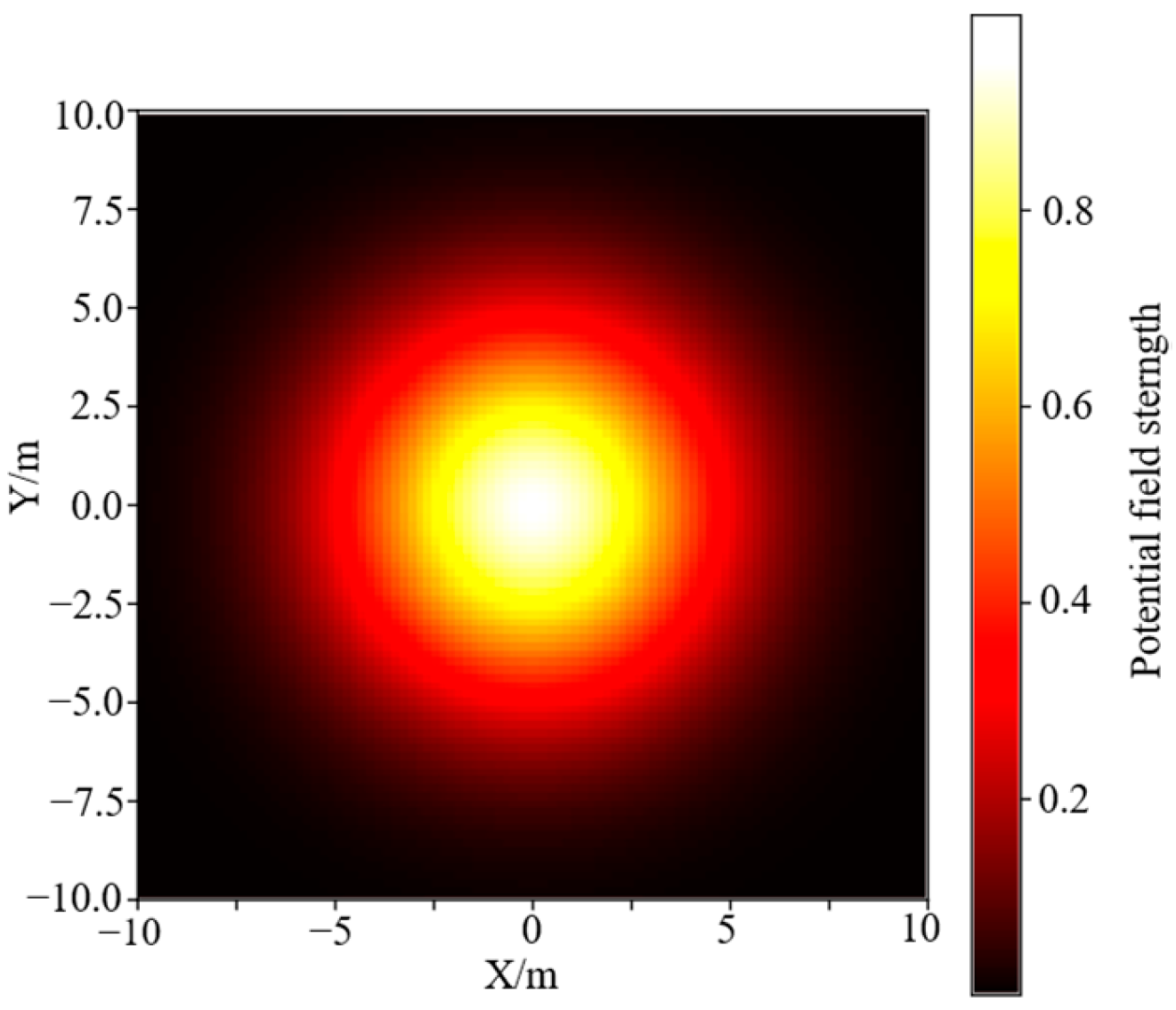
The boundaries of this risk potential field are relatively fixed. When a vehicle moves outside these boundaries, the interactive force exerted by the potential field diminishes rapidly. Visual representations of this risk potential field are provided in Figure 5 and Figure 6.

2.1.4. Asymmetric Pedestrian Risk Potential Fields

Analysis of pedestrian crossing and vehicle movement characteristics reveals that the pedestrian risk potential field exhibits asymmetry. Lateral risks within the pedestrian risk potential field significantly exceed longitudinal risks. Among lateral risks, the risk from oncoming vehicles far exceeds that from departing vehicles. Simultaneously, within longitudinal risks, the risk in the forward direction substantially surpasses that from the rear. Based on the characteristics of pedestrian crossing and vehicle operation [20], the primary objective of pedestrian crossing is to rapidly traverse the road to reach the opposite side. Regardless of their movement state (advancing or stationary), lateral risk is significantly greater than longitudinal risk. Among lateral risks, the risk from oncoming vehicles is far greater than that from departing vehicles. Simultaneously, among longitudinal risks, the risk in the forward direction is far greater than the risk in the backward direction. The pedestrian risk potential field should exhibit an asymmetric distribution.
Based on this, the asymmetric lateral dynamic pedestrian risk potential field is constructed as follows:
ψ H U M 1 = ω H 1 exp x λ x 1 2 + y λ y 1 2 + χ 1 ω H 2 x 2 λ x 1
where
ψ H U M 1 is the pedestrian lateral risk potential field;
ω H 1 , ω H 2 are the proportional adjustment coefficient of risk potential field;
x , y denote the differences in the lateral and longitudinal coordinates between the vehicle and the pedestrian, respectively, with a negative value indicating that the vehicle is to the pedestrian’s right ( χ 1 = 1 ), and vice versa for the left ( χ 1 = 0 );
λ   y 1 denotes the minimum longitudinal avoidance distance required by the vehicle, calculated as λ y 1 = v T min , where T min is the shortest obstacle avoidance time including driver reaction time;
λ x 1 indicates that the vehicle needs the shortest lateral obstacle avoidance distance:
ψ H U M 2 = ω H 2 exp x λ x 2 2 + y λ y 2 2 + χ 2 ω H 3 y 2 λ y 2 2
where
ψ H U M 2 denotes the longitudinal pedestrian risk potential field;
ω H 3 is the scaling coefficient for the potential field;
λ y 2 is the distance traveled by a pedestrian when a vehicle travels normally to the pedestrian, calculated as λ y 2 = x v · v h u m , where v h u m is the pedestrian’s walking speed.
Figure 7 and Figure 8 illustrate the variations within these asymmetric pedestrian crossing risk potential fields, demonstrating a significant increase in field intensity facing the direction of approaching vehicles compared to that from vehicles moving away. Similarly, the risk intensity facing the direction of pedestrian movement significantly exceeds that in the opposite direction. The field is thus segmented into lateral and longitudinal components. In the lateral segment, primary emphasis is placed on the side facing oncoming vehicles, allocating increased field intensity to allow for adequate deceleration and evasive maneuvers. Conversely, in the longitudinal segment, the focus is from the pedestrian’s perspective, ensuring that both pedestrians and vehicles, unaware of each other’s presence and maintaining constant velocities, can navigate the area safely. This necessitates a more pronounced field intensity in the direction of pedestrian travel compared to the opposite direction.

2.2. Quantification of Risk Fields in Two Dimensions on Roadways

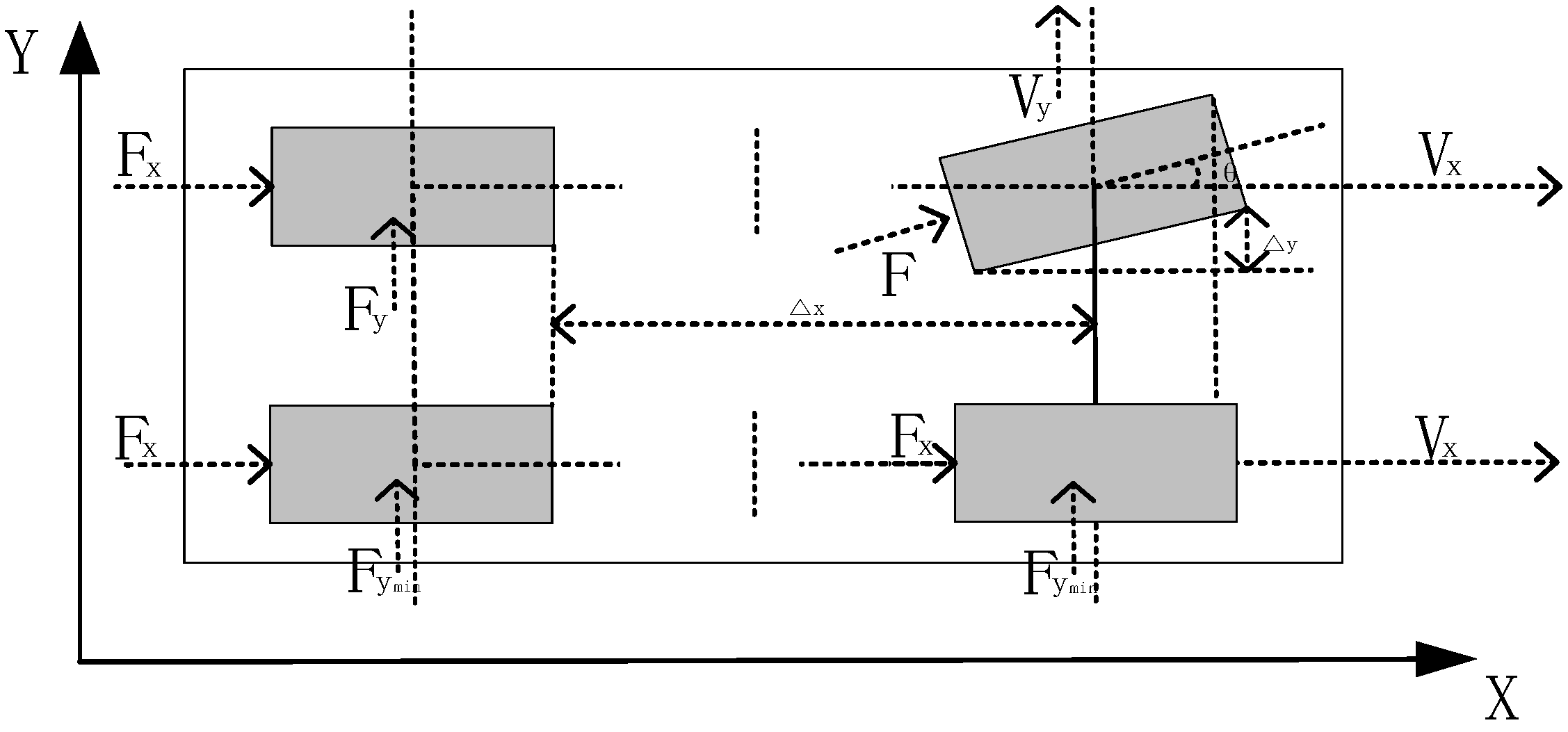
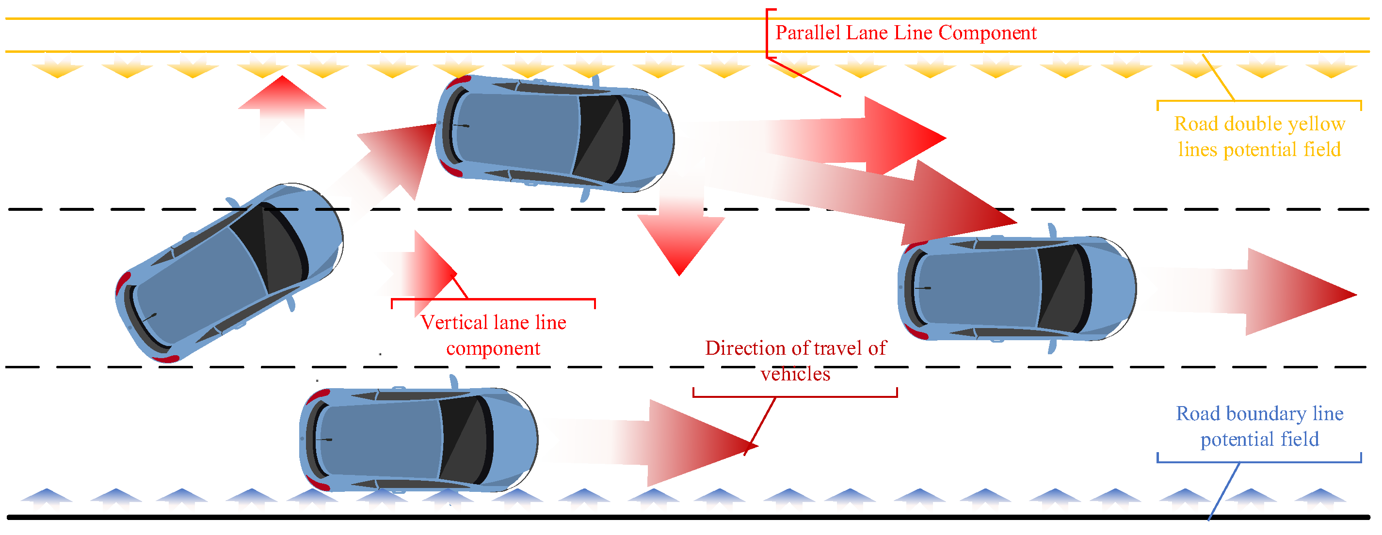
In practical scenarios, vehicular movement often deviates from a strictly longitudinal path, as illustrated in Figure 9.
This deviation in direction introduces a potential for interaction between the vehicle’s oblique trajectory and the pre-existing potential field. Within the established Cartesian coordinate system, the overall effective potential of the field is decomposed according to the directional vector. Specifically, the potential fields along lane markings and roadside boundaries are conceptualized as vector fields oriented along the y-axis, directed inward towards the center of the road. The interaction potential is then systematically decomposed in accordance with the directional vectors defined by the coordinate system.
ψ y = ψ * + ψ c · sin θ + ψ r + ψ l + ψ H U M
ψ x = ψ H U M + ψ * + ψ c · cos θ
Here, ψ y represents the y-axis component of the acting potential, ψ x represents the x-axis component of the acting potential, and γ is the clockwise angle between the vehicle’s direction of travel and the road’s centerline.

2.3. Optimization of Road Bottlenecks Based on the Driving Risk Field

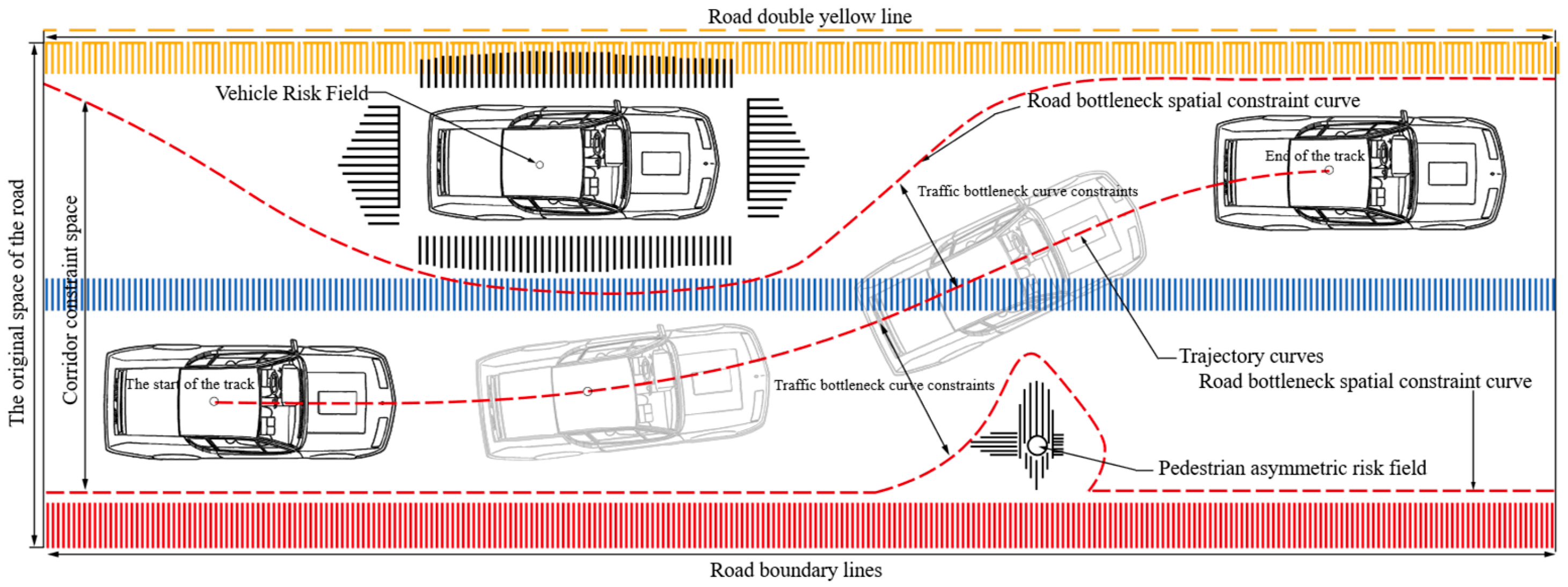
A road bottleneck is defined as a segment that becomes congested due to various traffic factors. In our approach, the quantified risk field is superimposed onto the existing road space, thereby constraining it to simulate the spatial configuration of a bottleneck area, as depicted in Figure 10.
As shown in Figure 10, the constraint curve of the traffic bottleneck area transforms the standard rectangular space, delineated by double yellow lines and road boundaries, into an irregularly shaped passable safety zone. The red dashed line in the figure delineates the constraint curve of the bottleneck area, defining the minimum and maximum bounds of potential vehicle trajectories. The red solid line illustrates the actual trajectory of the vehicle. The yellow area highlights the risk potential field associated with the double yellow lines, while the red area indicates the risk potential field of the road boundary. The blue area represents the centerline risk potential field. The trajectory generation adheres to the principle of following the steepest descent of the cost function gradient related to the bottleneck area constraints. The intensity of the risk potential fields progressively diminishes from red to blue, indicating a decrease in risk potential with distance from the road boundaries. A multi-objective driving risk potential field is constructed, focusing primarily on CAVs operating within traffic scenarios for trajectory planning. When making trajectory decisions, it is crucial to consider the variations in the surrounding risk potential fields, thereby excluding high-risk areas from the original road space to effectively form bottleneck areas. A trajectory curve, l = f s , is established, where sss represents the step count in the trajectory. Given the characteristic that the strength of the risk potential field decreases with distance, the trajectory curve l = f s is optimally positioned at the center of the bottleneck area at each step. Initially, the trajectory curve is subjected to an equality constraint.
Let l i = f s i , l i = f s i , l i = f s i , and assume the curve connecting l i and l i + 1 defined by f s is always l i + 1 l i Δ s . Taylor expansions are performed between l i and l i + 1 as follows:
l i + 1 = l i + l i Δ s + 1 2 l i Δ s 2 + 1 6 l i + 1 l i Δ s Δ s 3
l i + 1 = l i + l i Δ s + 1 2 l i Δ s + 1 2 l i + 1 l i Δ s Δ s 2
If A e q s r b = 1 Δ s Δ s 2 3 1 0 Δ s 2 6 0 1 Δ s 2 0 1 Δ s 2 , X = l 1 l 1 l 1 l n .
The equality constraint is then expressed as follows:
A e q s r b X = B e q s r b
Here, B e q s r b represents a zero matrix with 2 n 2 rows and 1 column.
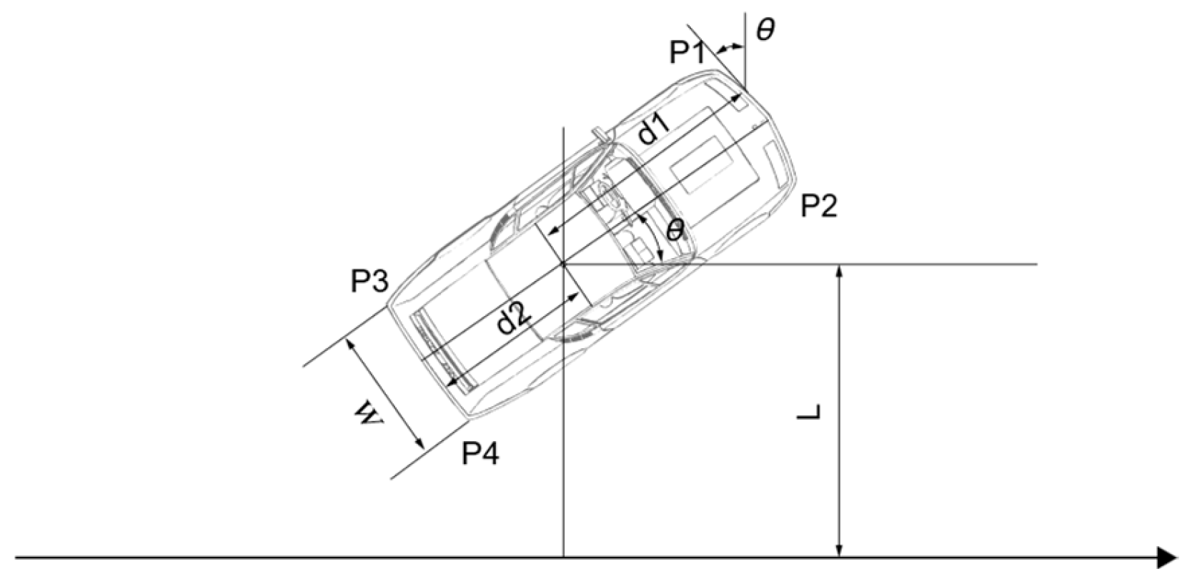
Initially, the trajectory curve is subjected to an equality constraint. Following this, inequality constraints generated by the road bottleneck areas are applied. Considering that a vehicle is not merely a point mass on the trajectory and possesses a collision volume, constraints are applied to the four corners of the vehicle.
As depicted in Figure 11, P 1 , P 2 , P 3 , and P 4 represent the four corners of the vehicle; d 1 is the distance from the vehicle’s center of mass to the front; d 2 is the distance from the vehicle’s center of mass to the rear; and W is the width of the vehicle. The constraints on the vehicle’s four corners are illustrated in the following equations:
l p 1 = l + d 1 sin θ + W 2 cos θ
l p 2 = l + d 1 sin θ W 2 cos θ
l p 3 = l d 2 sin θ + W 2 cos θ
l p 4 = l d 2 sin θ W 2 cos θ
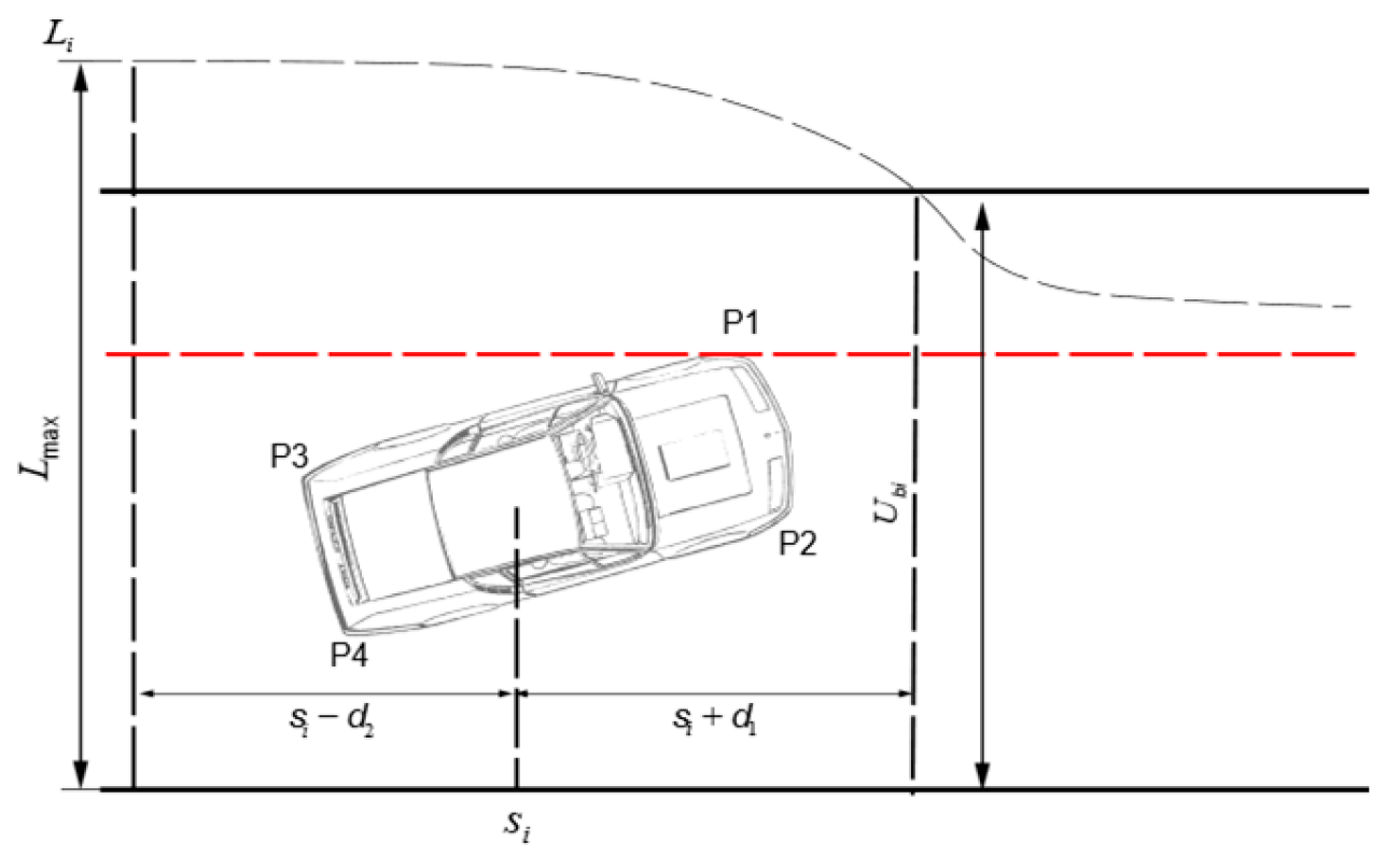
Setting sin θ = tan θ = l and cos θ = 1 , and as shown in Figure 12, we seek the minimum value of l max i within the interval s i d 2 , s i + d 1 , denoted as u b i . Similarly, the maximum value of l min i is denoted as l b i . The inequality constraints for the bottleneck area are established as follows:
l b i l p 1 u b i
l b i l p 2 u b i
l b i l p 3 u b i
l b i l p 4 u b i
These constraints are used to restrict the road space, and the trajectory cost function is designed as follows:
costfunction = W cos t r e f i l i 2 + W cos t d l i l i 2 + W cos t d d l i l i 2 + W cos t d d d l i l i + 1 l i 2 + W cos t m i d i l i l min i + l max i 2 2
where W cos t r e f is the cost for the road’s reference line, W cos t d l for the first derivative, W cos t d d l for the second derivative, W cos t d d d l for the third derivative, W cos t m i d for the central cost in the bottleneck area, and l i represents the position of the trajectory at step i , with l min i and l max i being the trajectory’s minimum and maximum constraints, respectively.
A simulation environment is constructed using Prescan 8.5.0 and Matlab/Simulink R2021a as shown in Figure 13 to validate the effectiveness of traffic bottleneck constraints across different road potential field scenarios.
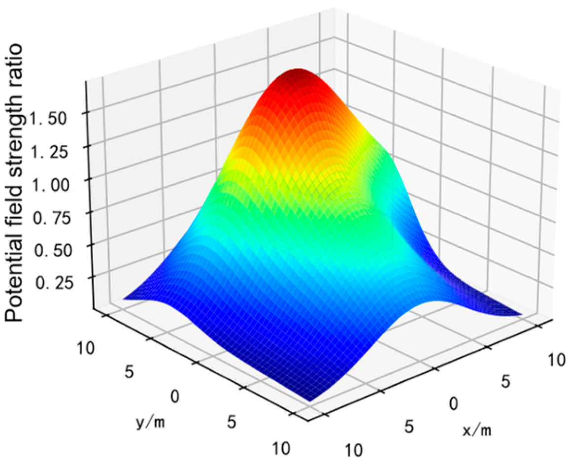
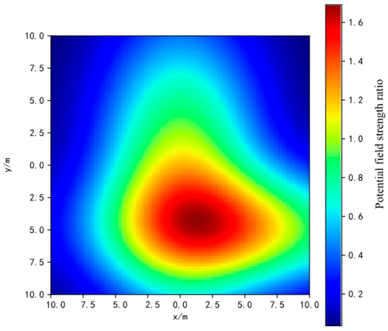
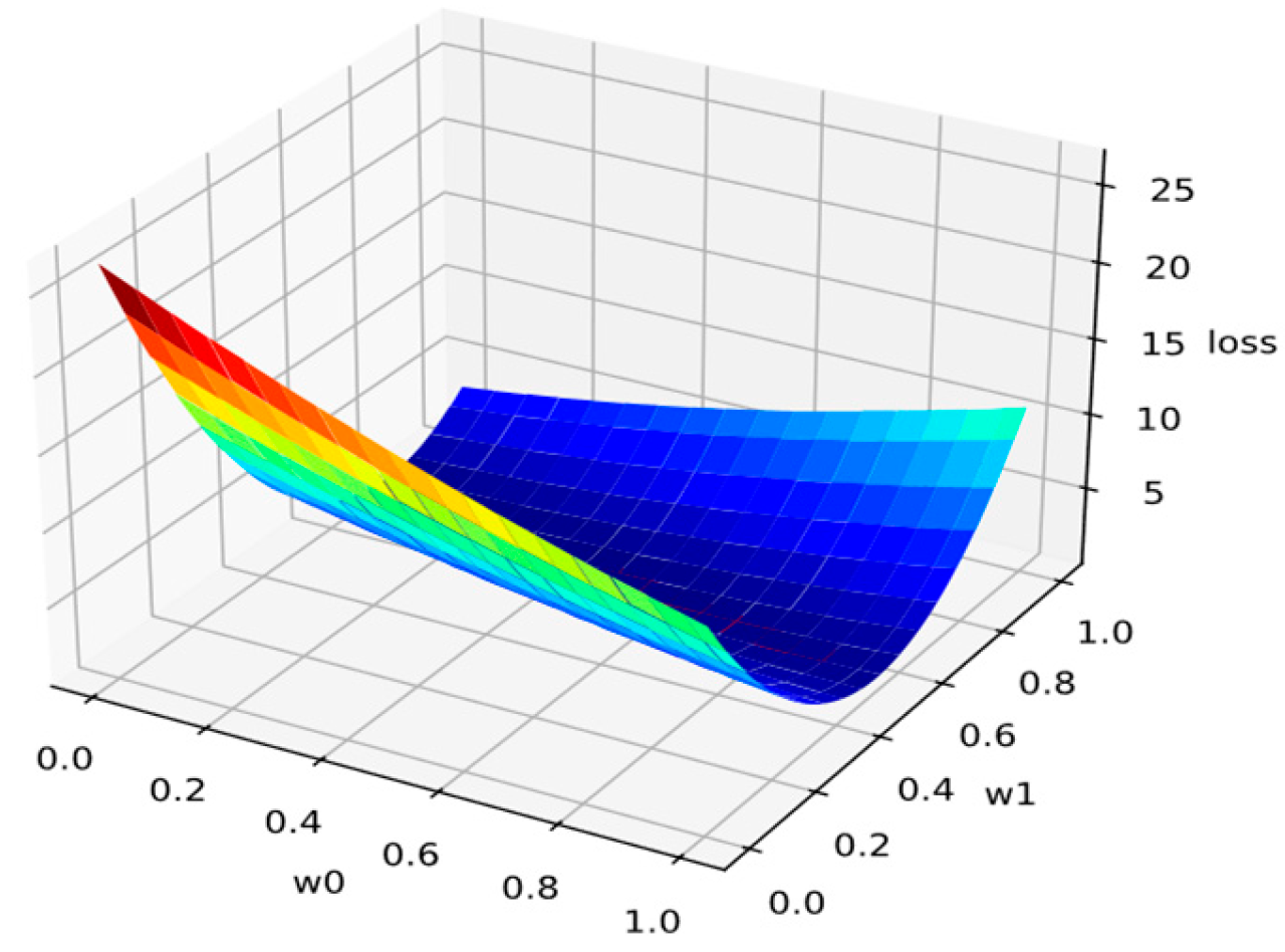
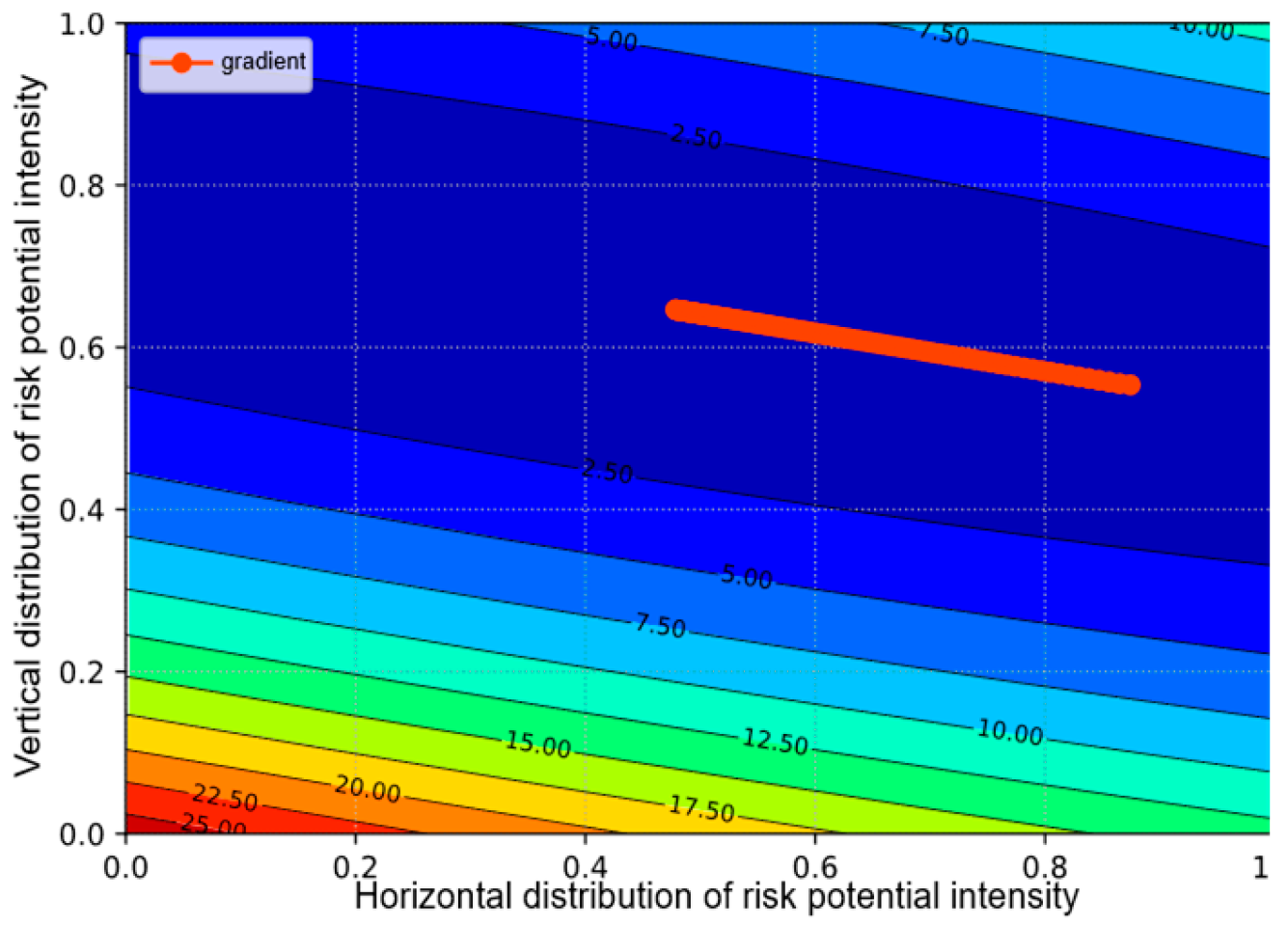
Upon optimization, the preliminary selection of parameters iteratively adjusts the trajectory along the gradient of lowest cost change, as shown in Figure 14 and Figure 15.

3. Vehicle Dynamics Model Construction

3.1. Vehicle Speed Stability

The vehicle’s speed potential energy at time t is denoted as P ( x , y ) t :
P ( x , y ) t = ξ x t · V y t
where P ( x , y ) t is the vehicle’s speed potential energy at time t , ξ x t is the lateral distribution coefficient at time t , and V y t is the vehicle’s speed at time t , measured in k m / h . The lateral distribution coefficients for different road lanes are shown in Table 2.
The direction of speed potential energy aligns with the trends in longitudinal speed and acceleration, pointing from lower to higher potential energy. Considering the typical design of roads in China, which are higher in the middle and lower on the sides, and the fact that the middle lanes have higher speeds than the outer lanes, a method for evaluating vehicle speed stability is established:
E y V E L = α · μ Δ P ( x , y ) d y
E x V E L = β μ Δ P ( x , y ) d x β μ Δ P ( x , y ) d x
α = 1.0 , i ¯ 2 % ; ( 100 ( i ¯ 1 ) , i ¯ 2 % .
E V V E L = E x V E L + k E y V E L
In these formulations:
Δ P ( x , y ) represents the difference in vehicle potential energy, expressed in km / h denotes the intensity coefficient of the velocity risk potential field.
α is the longitudinal risk impact factor.
β is the lateral risk impact factor.
i ¯ refers to the average longitudinal grade of the road segment, with i ¯ typically ranging from 2% to 3%.
d y and d x represent the longitudinal and lateral distances, respectively, directed from areas of higher to lower potential energy. d y is measured in km , and d x in m .
E y V E L indicates the intensity of the longitudinal velocity risk potential field.
E x V E L indicates the intensity of the lateral velocity risk potential field.
E V V E L denotes the strength of the velocity vector.
k is the coefficient for adjusting the direction of risk.

3.2. Stability of Vehicle Heading Angle

During maneuvers that involve lane changes, it is imperative to precisely control the magnitude of the vehicle’s steering angle. This control must be coordinated with the vehicle’s current speed and the varying conditions of the road. In congested road segments where vehicles are constrained to lower speeds, larger steering angles are typically employed. These larger angles enhance vehicular agility and improve traffic flow efficiency. Conversely, on open roads where vehicles can maintain higher speeds, smaller steering angles are utilized to ensure vehicular stability. This study delineates the relationship between steering angles and vehicle speed across different traffic conditions. It employs a motion model and a stability analysis method that accounts for changes in the kinetic energy associated with vehicle speed. Understanding this relationship is instrumental in defining the optimal entry angle for effective lateral vehicle control.
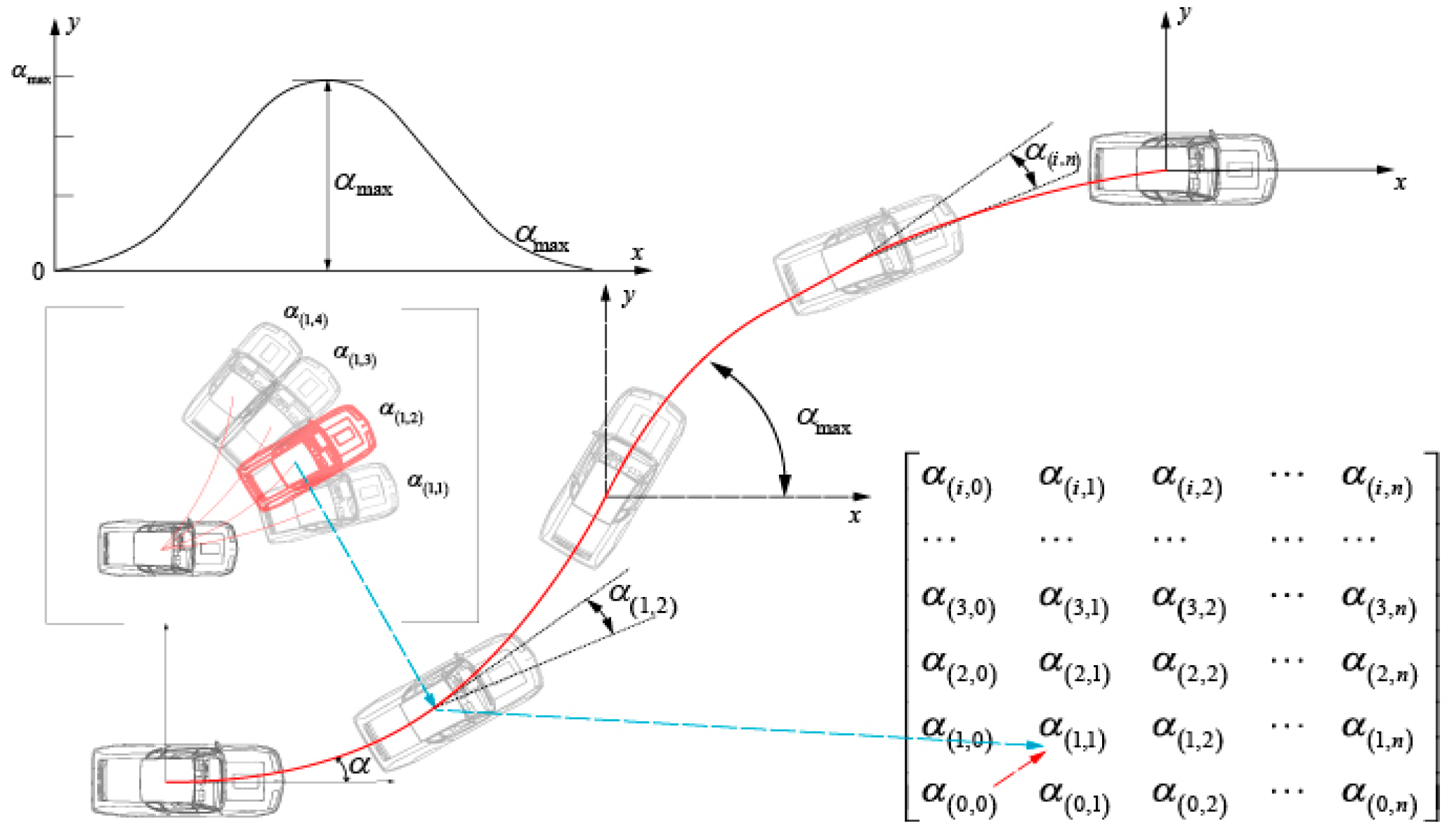
In scenarios where vehicles are part of a platoon, they exert a longitudinal force, F x , along the road direction. Under the influence of F x , a vehicle may move at a variable or constant speed along the road. Upon initiating a lane change, the vehicle is subjected to a lateral force, F y , perpendicular to the road direction. The action of F y facilitates the completion of the lane-changing maneuver. Consequently, the steering angle during the lane change correlates with the vehicle’s lateral and longitudinal displacement per unit time, as illustrated in Figure 16.
The longitudinal and lateral displacements of a vehicle per unit time are intrinsically linked to its respective longitudinal and lateral velocities. It thus becomes evident that controlling the vehicle’s steering angle fundamentally involves managing its longitudinal and lateral velocities. Prior to a lane change, while in a car-following state, a vehicle’s longitudinal velocity is typically zero. Upon initiating the lane change, the vehicle maintains this zero velocity but begins to experience a perpendicular acceleration relative to the vehicle’s orientation. Therefore, controlling the steering angle is tantamount to managing the vehicle’s longitudinal and lateral accelerations.
The acceleration of a vehicle profoundly affects passenger comfort, as summarized in Table 3. When the vehicle’s acceleration is below 1.8 m/s2 passengers experience high comfort levels, with minimal perception of the disturbances caused by changes in vehicle speed. When acceleration ranges between 1.8 m/s2 and 3.6 m/s2, passengers are subjected to a moderate comfort state, where changes in vehicle speed and resultant disturbances are noticeable but tolerable. Accelerations exceeding 3.6 m/s2 result in significant discomfort due to a pronounced perception of disturbances. Therefore, in the control of vehicle trajectory and speed, maintaining acceleration below 3.6 m/s2 is imperative to ensure both passenger comfort and vehicle stability.
As a vehicle progresses, its trajectory is continuous, and the heading angle changes accordingly. The function that describes the heading angle in relation to the time during lane-changing behavior is continuous and uninterrupted, capturing the variations in the entry angle throughout the lane change. Within a specific time interval, during maneuvers such as a lane change or obstacle avoidance, the closer the entry angle is to the current heading angle, the higher the comfort level experienced. This increased comfort is attributed to the stability of the angular velocity of the clockwise angle θ relative to time t. We define the ideal state heading angle as a function of velocity, formalized in Equation (27).
θ θ = arccos 1 1.8 v c 2
By employing this optimal entry angle function, the longitudinal acceleration of the vehicle can be adjusted based on its lateral acceleration, thus facilitating the transition to the optimal entry angle.

3.3. Calibration of Trajectory Stability Parameters

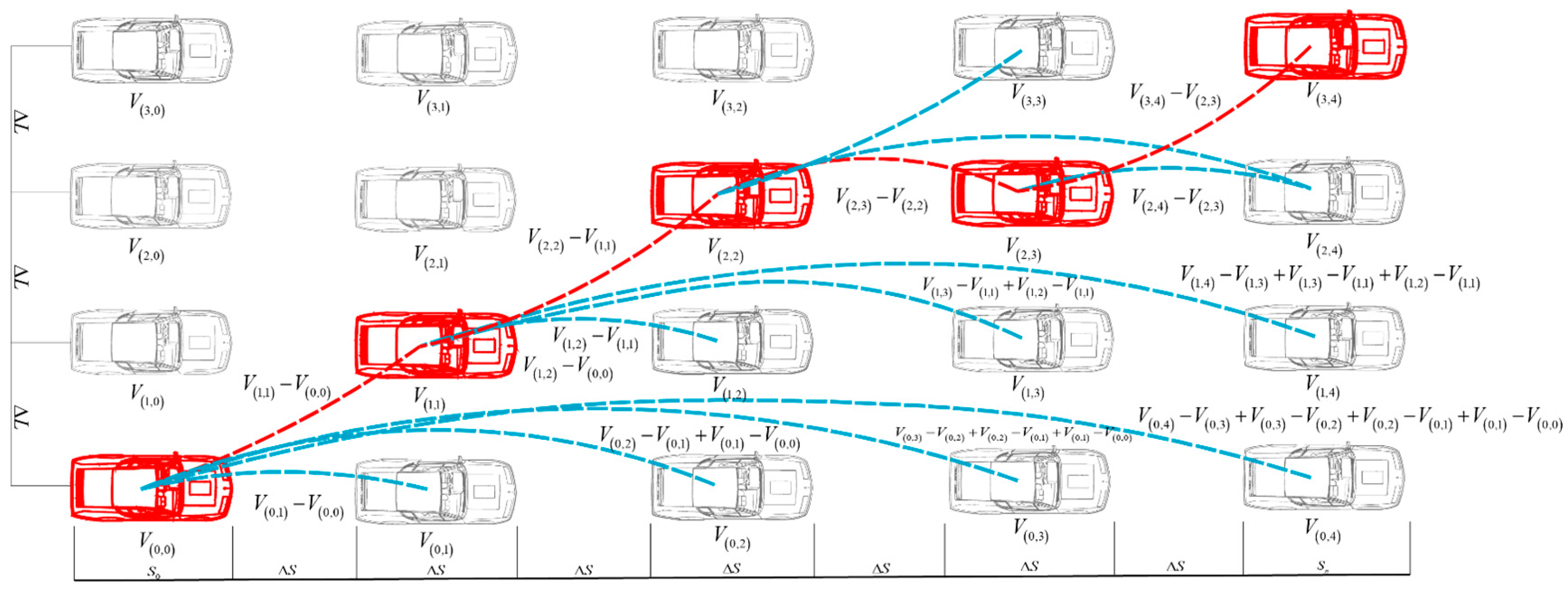
Based on the dynamics model of the vehicle, key stability indicators such as the heading angle, tilt, and changes in kinetic potential energy are selected to gauge the stability of the vehicular body. To quantify these indicators, as depicted in Figure 17, the vehicular environment is segmented into multiple road sections. For each segment, the kinetic potential energy is calculated using the designated formula. This process defines the feasible trajectories connected to the current road segment, culminating in a matrix of kinetic potential energy changes.
Select the path where the change in kinetic energy meets the requirements:
Δ V = Δ V d e s Δ V s t a Δ V d e s Δ V s t a 3.24
After selecting the path, further parameter calibration is performed based on the vehicle’s optimal approach angle:
As shown in Figure 18, starting from the vehicle’s initial position, the road’s centerline is utilized as the baseline for angles. Depending on the vehicle’s traveling speed, feasible angle intervals θ 1 2 , θ 1 3 are identified. From these intervals, the most appropriate angle θ 1 2 is selected to serve as the initial state of the vehicle. Using the direction of vehicle travel as a reference, feasible angle intervals are sought sequentially until the vehicle completes its lane change. In this context, the matrix of changes in kinetic potential energy in this section is denoted as V m × n , the tilt matrix as i ¯ m × n , and the heading angle matrix as θ m × n . Consequently, the vehicle stability parameter ω s t a b i l i t y is established, as defined in Equation (28).
ω s t a b i l i t y = V m × n i ¯ m × n θ m × n

4. Optimization of Vehicle Lane-Changing Trajectories Based on a Nonlinear Polynomial Model

4.1. Development of the Nonlinear Polynomial Model

Vehicle lane-changing trajectory optimization based on polynomial models typically employs parametric curves to describe trajectories. Compared to traditional autonomous driving trajectory algorithms, this approach offers advantages in intuitiveness, accuracy, and reduced computational complexity. To address the aforementioned requirements for safety, efficiency, and smoothness in lane-changing trajectories, a fifth-degree polynomial-based optimization method is proposed. This approach replaces the spline curve method—which requires multiple segment and node adjustments and may introduce discontinuities at junctions—with a more streamlined solution. Polynomial parameterization provides a compact and continuous representation. This compactness reduces the dimensionality of decision variables and enables efficient integration into the SQP framework. Furthermore, the closed-form derivatives of the polynomial explicitly impose spatial constraints derived from risk field evolution, ensuring both stability and comfort.
The function f X , Y , u is utilized to describe the vehicle’s trajectory, effectively representing the vehicle’s movement from its initial position to its target position. The function governing the vehicle lane-changing trajectory is defined as follows:
X ( u ) = i = 0 5 ω ( i , x ) u i = ω ( 0 , x ) + ω ( 1 , x ) u + ω ( 2 , x ) u 2 + ω ( 3 , x ) u 3 + ω ( 4 , x ) u 4 + ω ( 5 , x ) u 5 Y ( u ) = i = 0 5 ω ( i , y ) u i = ω ( 0 , y ) + ω ( 1 , y ) u + ω ( 2 , y ) u 2 + ω ( 3 , y ) u 3 + ω ( 4 , y ) u 4 + ω ( 5 , y ) u 5
where
u = t / t m ; t m denotes the duration of the vehicle lane change;
X ( u ) represents the vehicle’s lateral position in the Cartesian coordinate system;
Y ( u ) represents the vehicle’s longitudinal position in the Cartesian coordinate system;
ω ( 0 , x ) and ω ( 0 , y ) denote the initial lateral and longitudinal positions of the vehicle in the Cartesian coordinate system, respectively;
ω ( 4 , x ) , ω ( 5 , x ) , ω ( 4 , y ) , and ω ( 4 , y ) are trajectory adjustment parameters designed to prevent abrupt changes at specific points along the trajectory.
The control of the vehicle lane-changing trajectory primarily involves determining the values of ω i as illustrated in Figure 19. By imposing constraints on ω i , multiple clusters of vehicle trajectories can be generated.
Subsequent to the fitting of vehicle trajectory clusters with polynomial curves, the derivative of the generated fitting curve is computed to ascertain the slope of the curve. The vehicle’s initial and target positions are defined, and three constraint parameters are established. As a result, the fourth derivative of the polynomial curve is calculated, ensuring the fulfillment of the three parameter constraints. This process also guarantees the reasonableness and smoothness of the curve, with the design of vehicle trajectory adjustment parameters aiming to prevent sudden changes in the trajectory derivative, which could yield non-existent trajectory slopes and thus impact the trajectory planning outcome.
X ( 0 ) = X A , X ( 1 ) = X B Y ( 0 ) = Y A , Y ( 1 ) = Y B
X ( u ) = ω ( 1 , x ) + 2 ω ( 2 , x ) u + 3 ω ( 3 , x ) u 2 + 4 ω ( 4 , x ) u 3 + 5 ω ( 5 , x ) u 4 X ( u ) = 2 ω ( 2 , x ) + 6 ω ( 3 , x ) u + 12 ω ( 4 , x ) u 2 + 20 ω ( 5 , x ) u 3 X ( u ) = 6 ω ( 3 , x ) + 12 ω ( 4 , x ) u + 60 ω ( 5 , x ) u 2 X ( u ) = 12 ω ( 4 , x ) + 120 ω ( 5 , x ) u
Y ( u ) = ω ( 1 , y ) + 2 ω ( 2 , y ) u + 3 ω ( 3 , y ) u 2 + 4 ω ( 4 , y ) u 3 + 5 ω ( 5 , y ) u 4 Y ( u ) = 2 ω ( 2 , y ) + 6 ω ( 3 , y ) u + 12 ω ( 4 , y ) u 2 + 20 ω ( 5 , y ) u 3 Y ( u ) = 6 ω ( 3 , y ) + 12 ω ( 4 , y ) u + 60 ω ( 5 , y ) u 2 Y ( u ) = 12 ω ( 4 , y ) + 120 ω ( 5 , y ) u
where X ( 0 ) , Y ( 0 ) represent the initial lateral and longitudinal positions of the vehicle, and X ( 1 ) , Y ( 1 ) denote the target lateral and longitudinal positions for the vehicle’s lane change.
The parameters influencing the lane-changing model include ( X A , Y A , ω ( i , x ) , θ A ) and ( X B , Y B , ω ( i , y ) , θ B ) . According to the requirements for the lane-changing trajectory, these parameters must be calibrated as follows:
(1) The vehicle’s heading angle at the initial lane-changing position, θ A = 0 , is set to 0, and at the target lane-changing position, θ B = 0 , is also set to 0.
(2) The curvature of the vehicle’s trajectory at both the initial and target lane-changing positions is set to zero.
(3) During the lane change, the trajectory generation must comply with the stability parameters, denoted as ω s t a b i l i t y .
(4) In compliance with national road construction standards, the lateral travel distance within the lane is set at 3.75 m.
Based on the aforementioned formulas and constraints, the unknowns within the trajectory model, ω ( i , x ) , ω ( i , y ) , X B , Y B , θ , can be calibrated. The objective function for parameter optimization involving vehicle trajectories is given by the following:
f ω ( i , x ) , ω ( i , y ) = min ( ω s t a b i l i t y Δ s sin θ + ω s t a b i l i t y Δ s cos θ )
where Δ s represents the differential element of the lane-changing trajectory length, with s being s = 0 u X ( u ) . 2 + Y ( u ) . 2 d u .
With the above conditions ensured, parameter constraints for the stability of the trajectory are established, where the curvature of the trajectory can be expressed as follows:
K ( Δ u ) = X ( Δ u ) Y ( Δ u ) X ( Δ u ) Y ( Δ u ) X ( Δ u ) 2 + Y ( Δ u ) 2 3 / 2
where K ( Δ u ) represents the slope at point Δ u along the curve.
The constraints on trajectory stability are such that under the premises of meeting the specified vehicle trajectory objectives, changes in trajectory curvature should be minimized:
K = min ( ω s t a b i l i t y R ) E K ( Δ u ) = K i j
where R is a matrix in the range (0,1); the matrix point value corresponding to the angle that meets the requirements of Equation (35) is 1, and 0 otherwise; and E is the unit matrix.
After satisfying the two aforementioned equations, a final selection among the remaining clusters of trajectories is conducted based on system throughput efficiency and vehicle passage efficiency:
V ( u ) = max ( 0 t m ( X ( u ) + Y ( u ) ) d v i = 0 n X ( i ) )
where X i represents the delay in traffic efficiency caused by lane-changing activities of vehicles queuing in the target lane; n denotes the number of vehicles queuing in the target lane.
The objective function described above constitutes a nonlinear programming problem. This study employs Sequential Quadratic Programming (SQP) as its core optimization framework. The trajectory planning task involves nonlinear vehicle dynamics, multi-source risk field constraints, and the synergistic optimization of safety, stability, and comfort. The SQP algorithm transforms the original complex nonlinear optimization problem into a series of subproblems approximated by quadratic programming at each iteration point. By solving the quadratic subproblem to obtain a new solution point, the original problem is then approximated using quadratic programming at this new point. Unlike Model Predictive Control (MPC), which requires repeated optimization at each control step, SQP solves the problem only once per planning cycle, thereby reducing computational cost and enhancing real-time performance. Furthermore, vehicle dynamics constraints and spatial constraints based on driving risk fields can be explicitly incorporated into the SQP optimization process. The specific procedure is as follows:
There exists a constrained nonlinear programming problem of the following form:
min y ( x ) G i ( x ) = 0 ( i = 1 , 2 , 3 , , n e ) g i ( x ) 0 ( i = n e + 1 , n e + 2 , n )
where x is the vector to be optimized, x = x 1 , x 2 , x 3 , , x n , and for i n e + 1 , n e + 2 , n , g i ( x ) represents inequality constraints and G i ( x ) represents equality constraints.

4.2. Solution of Nonlinear Polynomial Models Using the SQP Method

The SQP algorithm solves subproblems through a quadratic approximation of the Lagrange function:
L ( x , λ ) = y ( x ) + i = 1 m λ i g i ( x )
Here, λ i represents the Lagrange multipliers.
By concurrently linearizing and non-linearizing the constraint conditions, the SQP subproblem related to the original problem can be formulated, with the objective function described as follows:
min d R * 1 2 d T H k d + ( y ( x k ) ) T d
In this formulation: d represents a global variable; denotes the gradient; and H k is the Hessian matrix of the Lagrange function, approximated using a quasi-Newton method. The constraints of the objective function are as follows:
( g i ( x ) ) T d + g i ( x ) = 0 ( i = 1 , 2 , 3 , n e ) ( g i ( x ) ) T d + g i ( x ) 0 ( i = n e + 1 , n e + 2 , , n )
The solution to the problem is calculated using a semi-definite Newton approximation method, and is represented in the new iterative equation as follows:
x k + 1 = x k + a k d k
Here, d k is a vector pointing from x k towards x k + 1 , and a k is a scalar step size determined during a line search to ensure a sufficient reduction in a specified performance function.
The SQP algorithm is widely acknowledged as a highly effective method for addressing nonlinear optimization problems. In comparison to conventional algorithms, SQP offers numerous merits such as excellent convergence characteristics, superior computational efficiency, and robust capability in boundary searching. Accordingly, this study utilizes the SQP method to optimize trajectory parameters and presents the outcomes of the nonlinear optimization challenge.
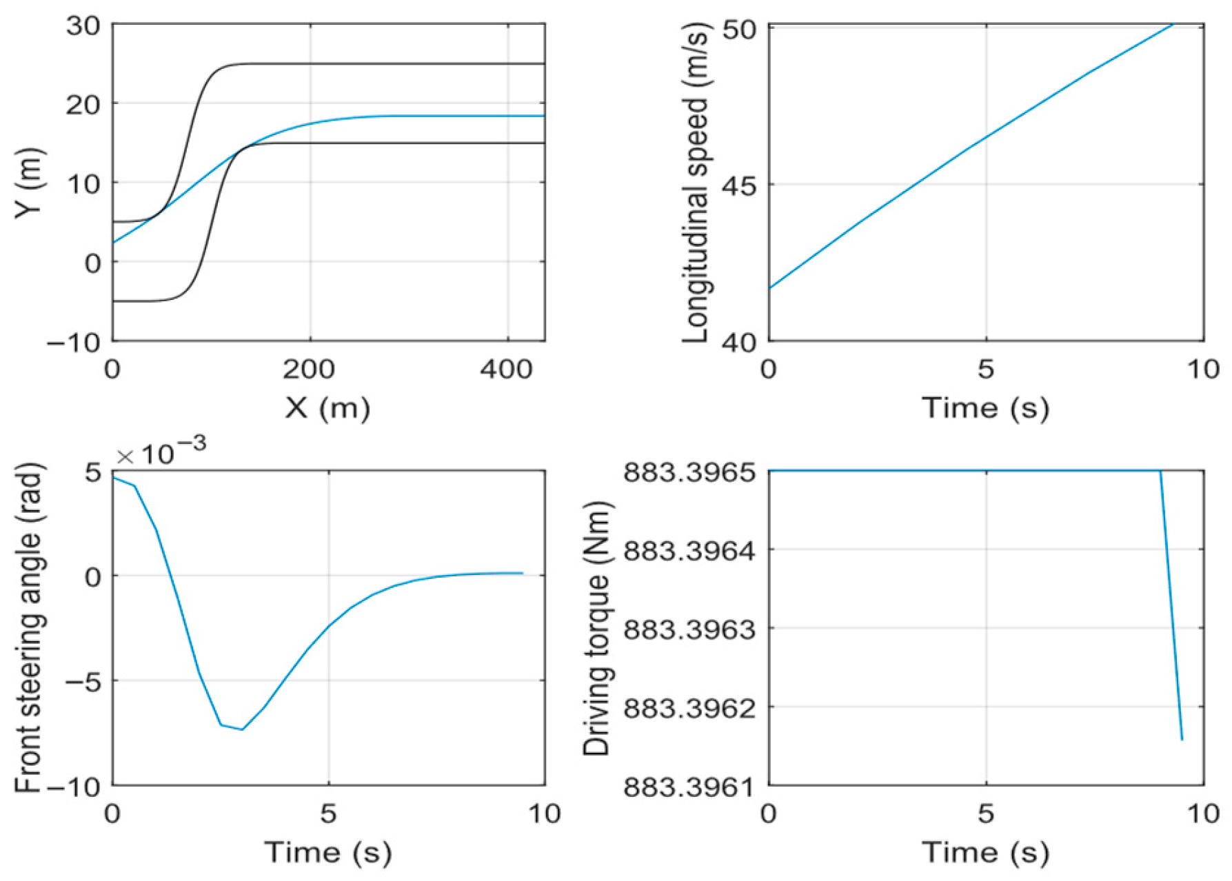
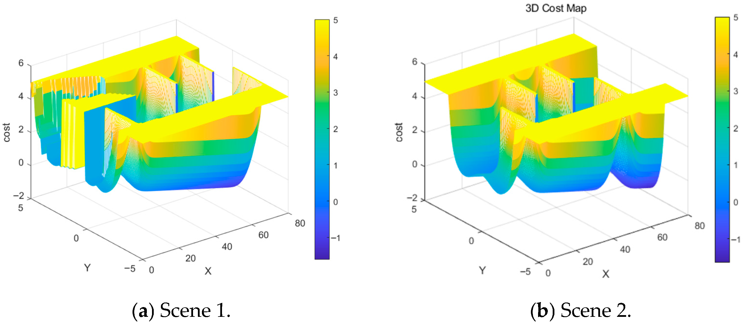
To demonstrate the practicality of the method, the curve-function-fitting vehicle trajectories are solved. To reduce the computation time for trajectory curves while ensuring smoothness and symmetry in lane-change curves, the target curve function is solved by setting and specifying zero acceleration at both the initial and final positions. It should be noted that despite using a simplified quintic polynomial, this approach differs fundamentally from directly employing a cubic polynomial. First, the quintic polynomial possesses six free coefficients, enabling simultaneous satisfaction of position, velocity, and acceleration boundary conditions at both the start and end points of the trajectory. In contrast, the cubic polynomial has only four coefficients, incapable of fully characterizing acceleration boundary constraints. Second, the quintic polynomial explicitly provides an expression for acceleration change rate (acceleration rate), enabling the implementation of comfort constraints related to acceleration changes. Finally, the quintic polynomial is structurally compatible with the Sequential Quadratic Programming (SQP) framework, allowing flexible utilization of higher-order terms for optimization when nonlinear dynamics or safety constraints are present. Lane changes were performed with initial vehicle speeds of 30 km/h, 40 km/h, and 50 km/h. The optimized curve solutions are presented in Table 4. As shown in the table, the algorithm achieves an average iteration time of 5.29 s, demonstrating high computational efficiency. While the curve curvature meets stability requirements, the degree of constraint violation gradually decreases with increasing iterations. This indicates that the vehicle trajectory curve progressively approaches a reasonable trajectory curve within the specified range. This is illustrated in Figure 20.

5. Simulation Experiments and Result Analysis

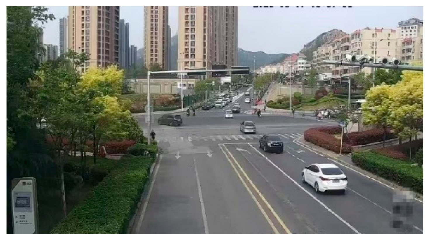
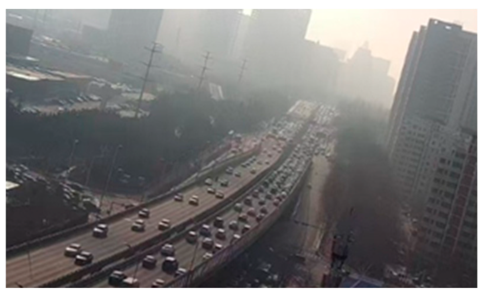
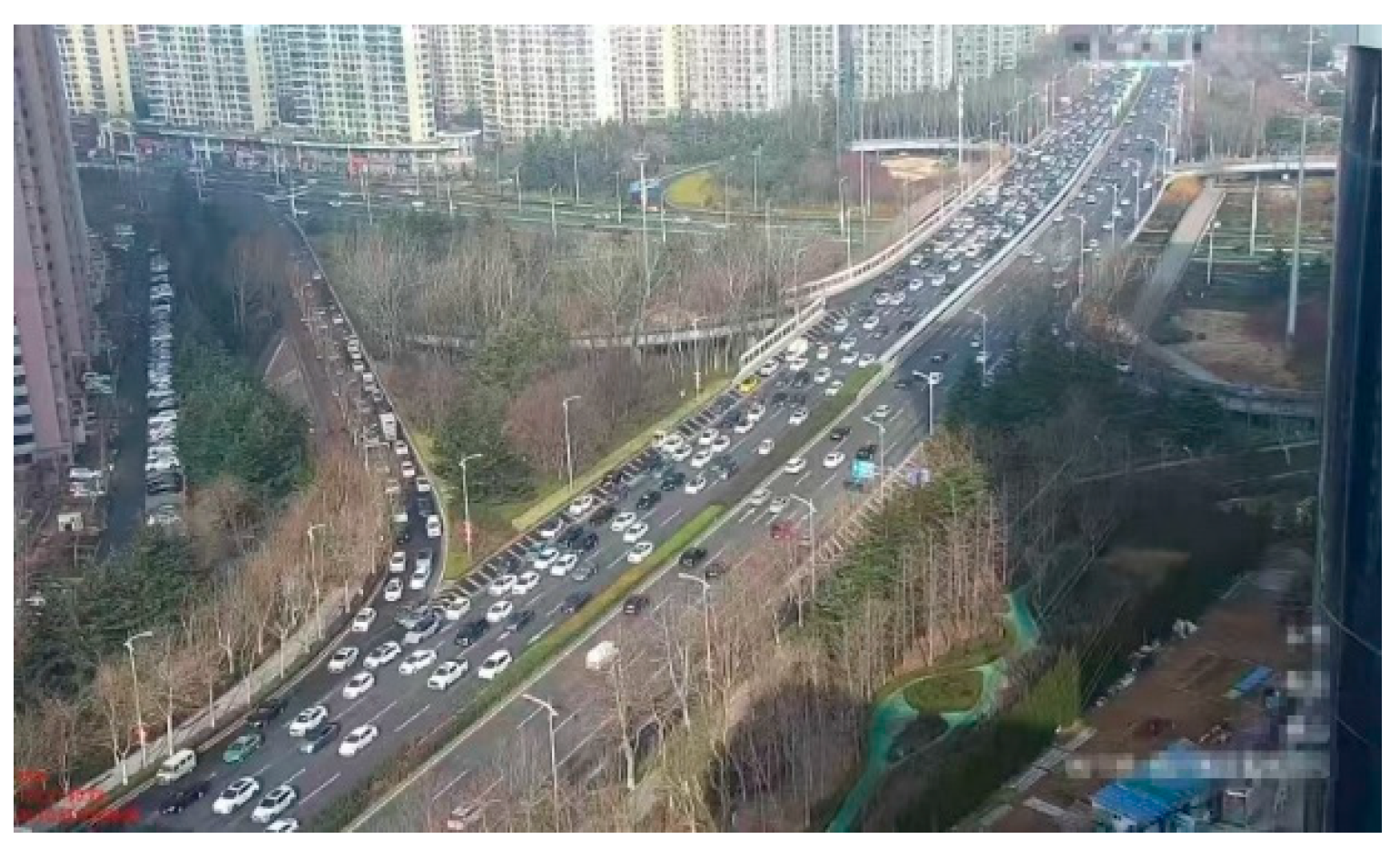
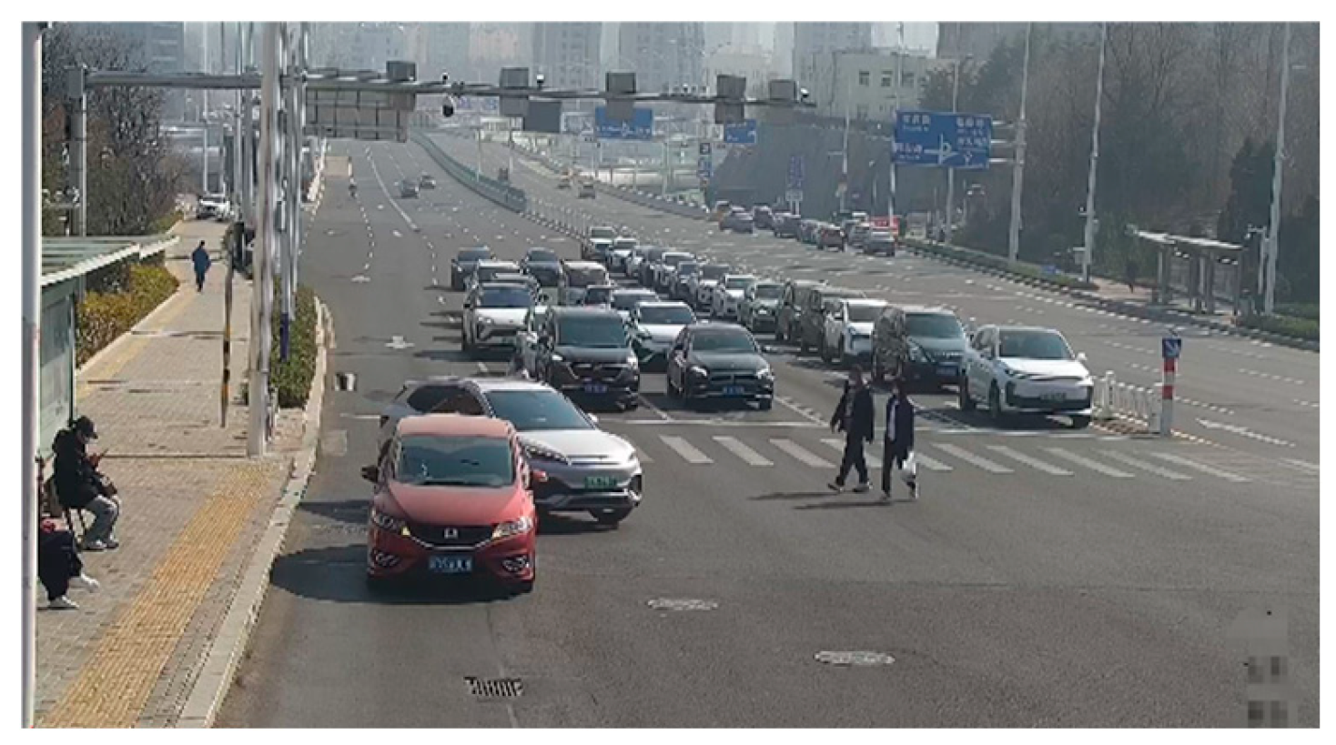
The model’s reference data are based on a general dataset, combined with real-world video datasets, and utilize authentic datasets from actual scenarios for testing and simulation. The figure below depicts a real-world data collection scenario, specifically a mixed traffic environment on an urban expressway. After collecting scenario data, this scenario was simulated and tested within a simulation environment. We validated the results using data from real traffic scenarios, sourced from real-world traffic camera video data, as shown in Figure 21 and Figure 22:
In addition to utilizing the High-D dataset and NGSIM dataset for vehicle risk fields and employing generic data such as pedestrian crossing feature data from the Paddle platform for pedestrian risk fields, we also incorporated real video data for calibration and validation of vehicle risk fields and asymmetric pedestrian risk fields. This shown in Figure 23 and Figure 24.
The control of vehicle trajectories has been implemented using an optimized MPC controller. MPC is fundamentally a state-space-based optimal control method designed to optimize a control sequence over a finite time horizon, aiming to align the system state as precisely as possible with the desired trajectory. During each control cycle, the MPC algorithm computes an optimal solution based on current states and a predictive model, thereby determining the most effective control strategy for the subsequent period. Only the first control action from this sequence is executed. In the following control cycle, the algorithm reevaluates and optimizes, thus achieving closed-loop control. The control process is structured as follows:
(1) Develop an appropriate mathematical model for the monitored object to serve as a predictive model, describing its future states.
(2) Set the control function within the SQP trajectory optimization algorithm to optimize the trajectory of the monitored object according to the defined optimization objective.
(3) Define constraints for the objective function, calculating control parameters from the initial conditions to bring the monitored object closer to the reference state.
(4) Apply these control parameters to the execution module. As the system progresses to the next sampling moment, it reassesses the initial state and repeats the aforementioned steps for rolling optimization. The simulation parameters are presented in Table 5.
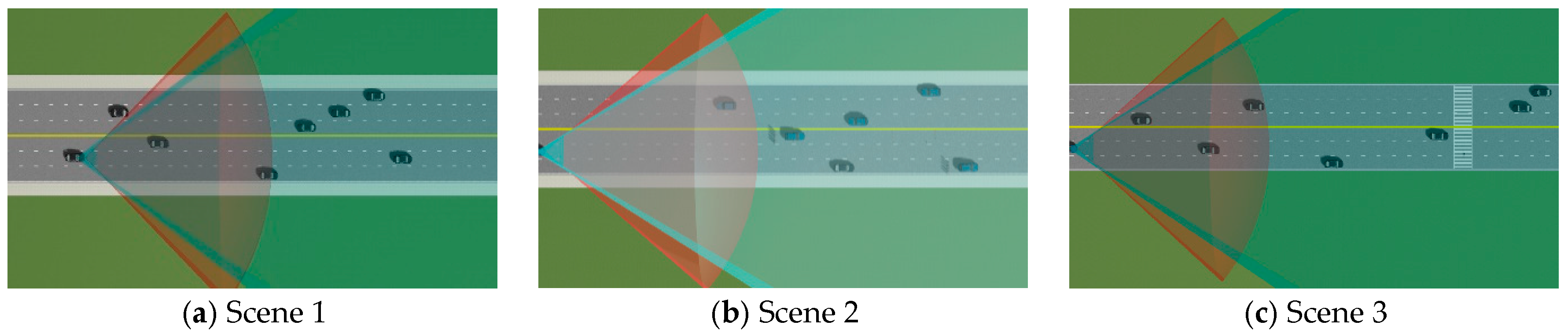
Simulation Scenario 1 is configured as follows: The lead vehicle enters an on-ramp at an initial velocity of 40 km/h. Owing to the constraints imposed by the freeway interchange, a compulsory lane change into the main roadway is necessitated. The path for the lane change is complicated by the presence of multiple obstructive vehicles, offering opportunities to merge into either Lane 1 or Lane 2. In Lane 1, obstructive vehicles CAV1 and CAV2 are positioned, while CAV3 and CAV4 are located in Lane 2.
Simulation Scenario 2 is delineated as follows: Operating in Lane 2 at an initial velocity of 40 km/h, the lead vehicle prepares for a lane change. The lane change trajectory intersects four obstructive vehicles: CAV1 and CAV4 in the adjacent Lane 2 and CAV2 and CAV3 in Lane 1. The proximities to these vehicles are detailed in Table 6.
The construction of each specific simulation scenario is illustrated in Figure 25, and the distribution status of the risk potential field in each scenario is depicted in Figure 26.
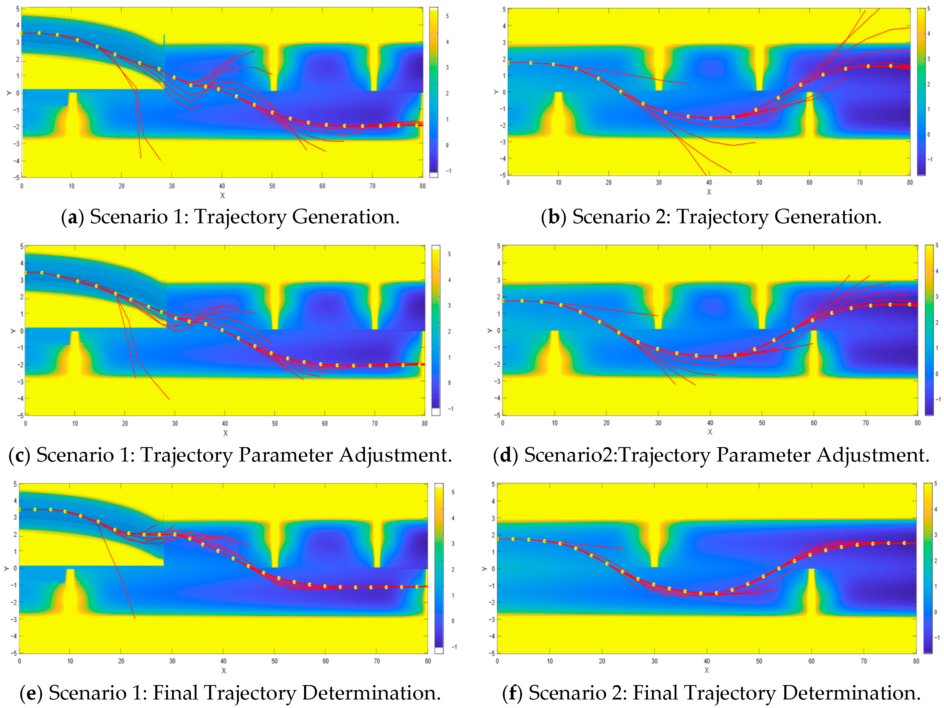
In scenarios involving four predefined obstructive vehicles, the intensity of the potential field is set to infinity when a vehicle is at the road boundary or proximate to an obstacle. The trajectory planning algorithm is employed to design the movement trajectory of the main vehicle. The generation and selection of trajectory clusters are subject to a functional assessment, as depicted in Figure 27. The trajectory refinement process entails adjustments to parameters for trajectories that surpass predefined constraints, thereby ensuring that the selected trajectory curves are smooth and continuous.
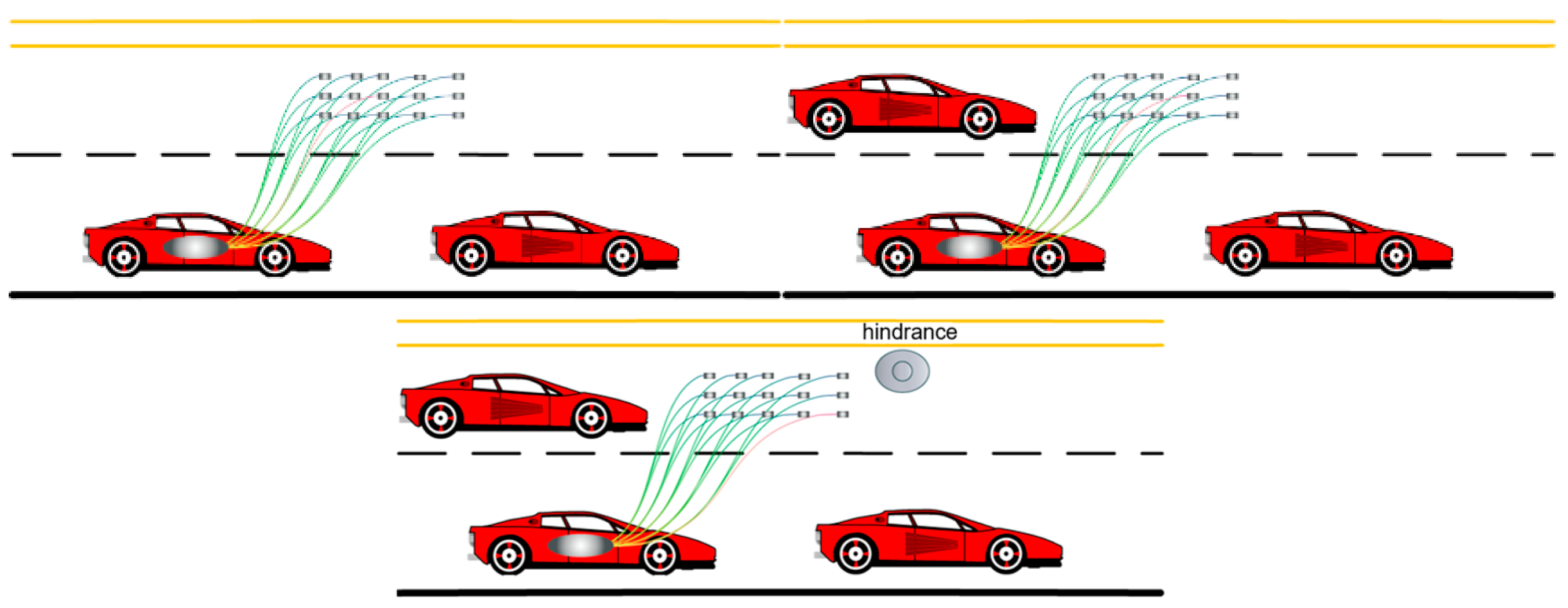
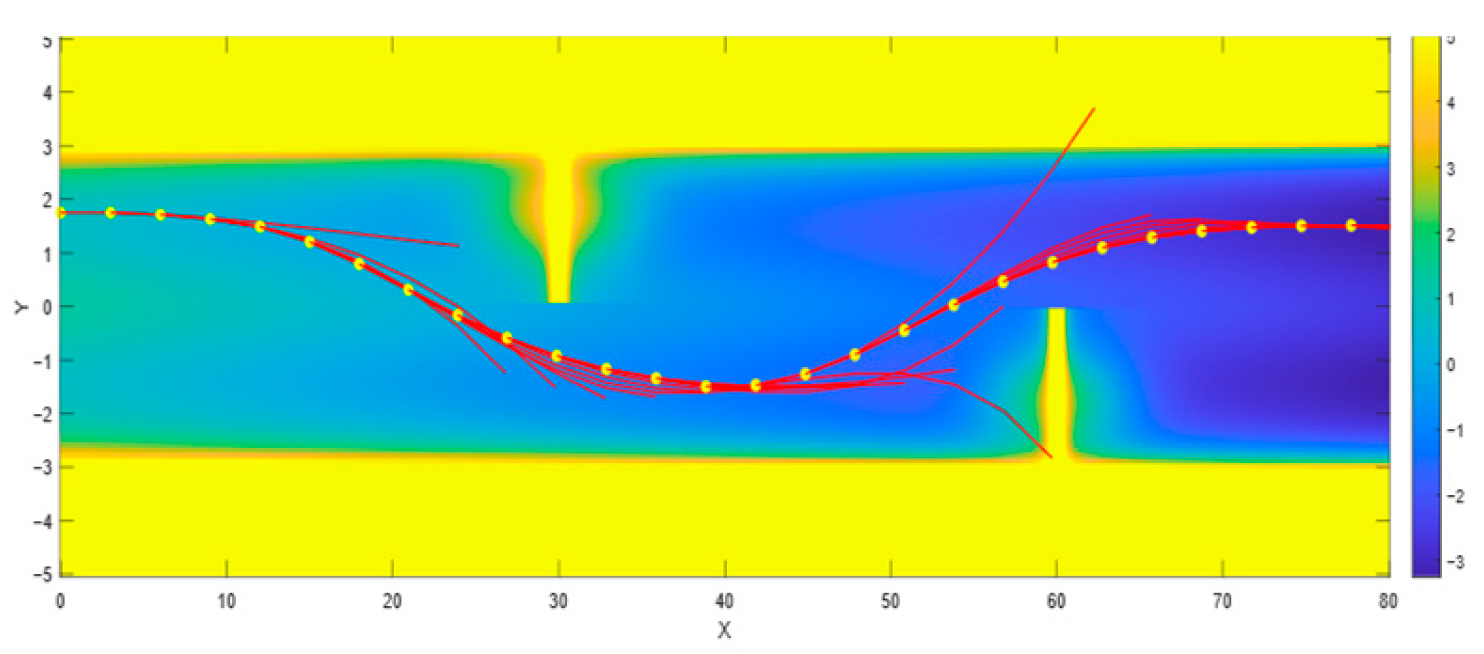
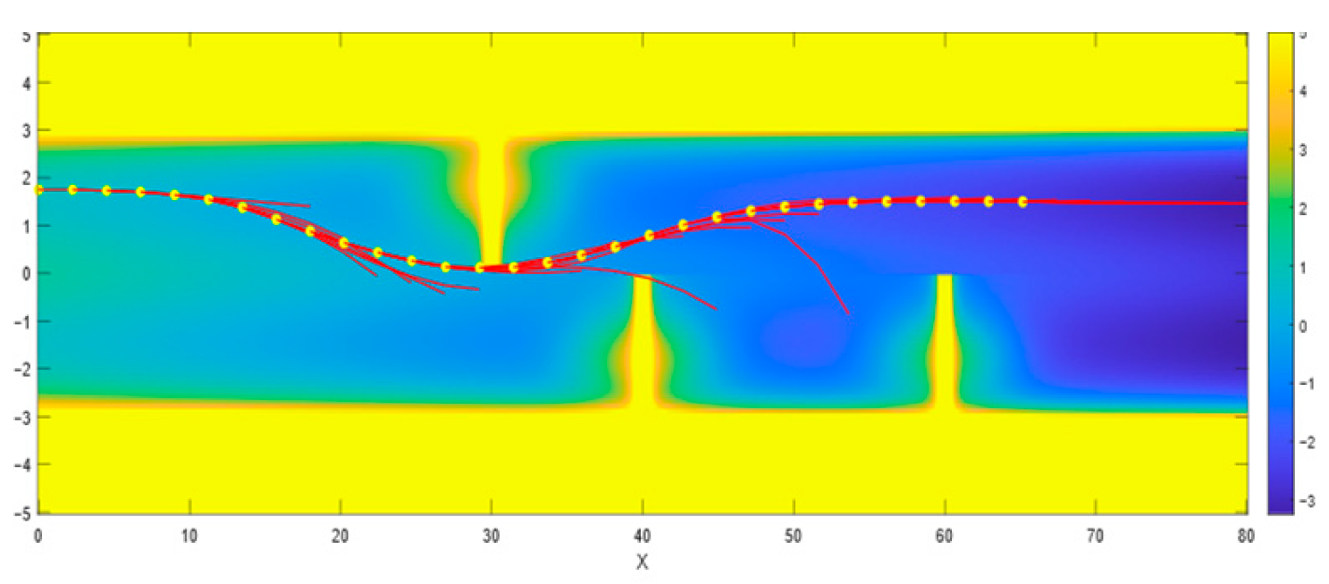
To validate the advantages of the Driving Risk Field in quantifying road spatial constraints, we conducted ablation experiments. The experiments comprised two main parts: the Driving Risk Field ablation study section performed dual tests on key simulation scenarios with identical initial conditions—once with full Driving Risk Field constraints enabled and once with them disabled; the partial risk field ablation study section demonstrated the contribution of individual components by removing single risk fields. The experimental results are shown in Figure 28 and Figure 29. The findings indicate that the “driving risk field” continues to demonstrate trajectory optimization effects even within the ablation experiments.
In the process of trajectory generation, it can be seen from Figure 22 that after adjusting the polynomial parameters, the trajectory curve of the vehicle is getting closer and closer to the optimal trajectory curve. By manipulating variables such as market weight, incremental weight, and acceleration thresholds, trajectory parameters are adjusted. The optimized method demonstrates significant enhancements over traditional control algorithms, including LQR, MPC, and PP algorithms. These improvements are evidenced in subsequent figures.
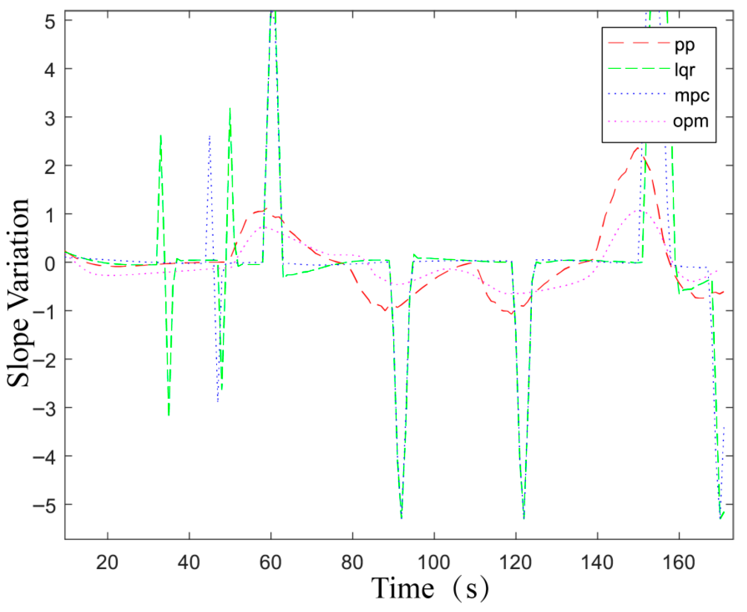
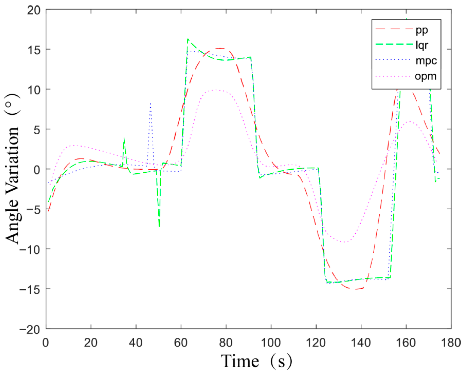
Figure 30 illustrates the variation of the vehicle’s heading angle over a simulation step time under the trajectory optimization algorithm. Figure 31 shows the slope of the heading angle variation along the trajectory. Compared to the baseline models (LQR, MPC, PP), the proposed model reduces the average trajectory angle slope by approximately 17.9%. Both metrics exhibit fluctuations within reasonable ranges, satisfying the stability constraints of the vehicle trajectory. Compared to other traditional algorithms, the optimized algorithm achieves smoother transitions in heading angle switching and angular change rates, aligning more closely with the vehicle’s optimal trajectory. Simultaneously, the trajectory angle slope directly corresponds to the vehicle’s angular velocity. Lower angular velocity translates to reduced lateral centrifugal forces during lane changes and obstacle avoidance, effectively enhancing ride comfort. Furthermore, lower angular velocity significantly diminishes the vehicle’s disturbance to overall traffic flow, thereby improving local flow stability and increasing average traffic efficiency.
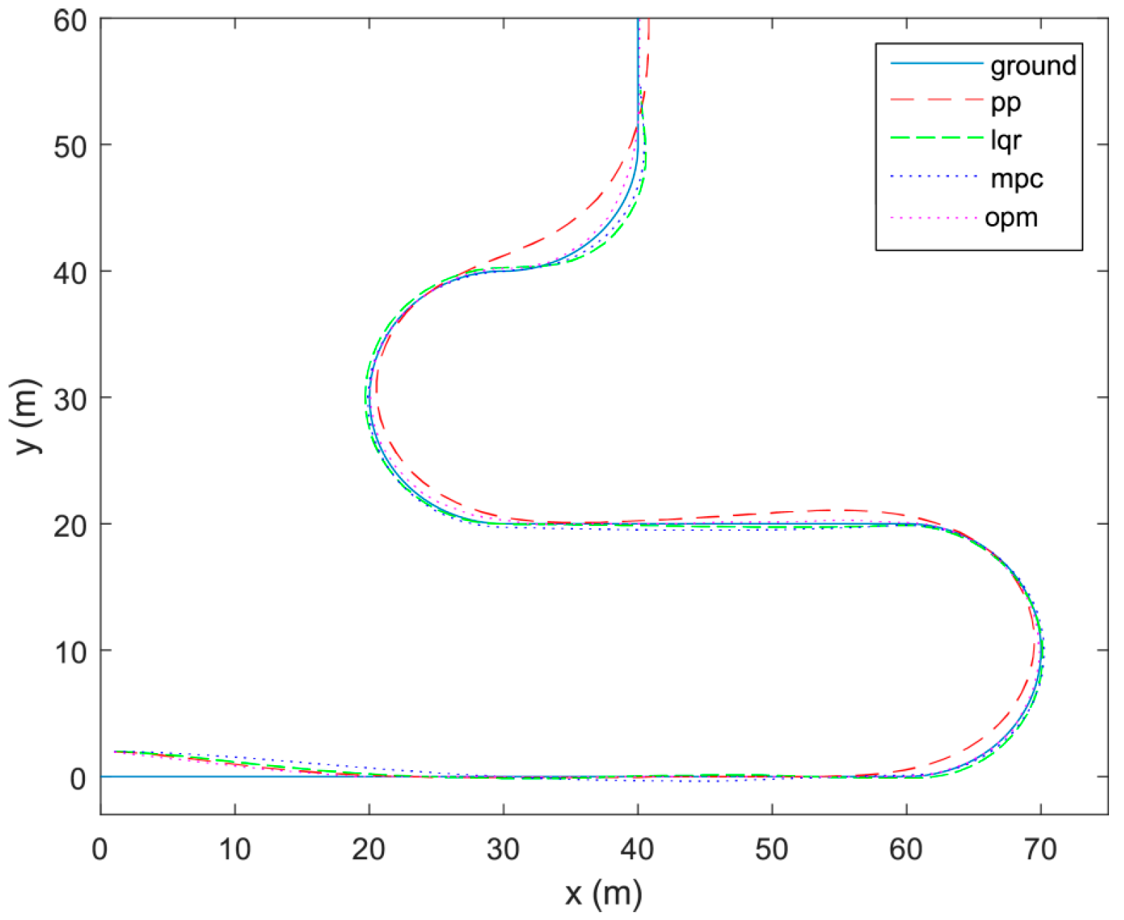
Figure 32 contrasts the vehicle trajectories under the trajectory optimization algorithm with those derived from traditional control methods. The trajectory generated by the optimized algorithm more closely matches the predefined optimal trajectory, indicating a higher adherence to trajectory optimization constraints. The optimized results are validated in groups by RMSE means, and the validation results are shown in Table 7.
p-values were calculated based on the F-method test, and the p-value was set at 0.05 as the threshold for significant difference. A total of 50 samples were selected for the test, and the comparison of p-values of RMSE for different methods is shown in Table 8.
Using a p-value of 0.05 as the significant difference threshold, both MPC and LQR are not significantly different from this paper’s method in terms of p-value comparisons, but they are improved by approximately 7.5% and 10.7%, respectively, relative to the RMSE mean, and thus, in comparison, this paper’s method still has some advantages.
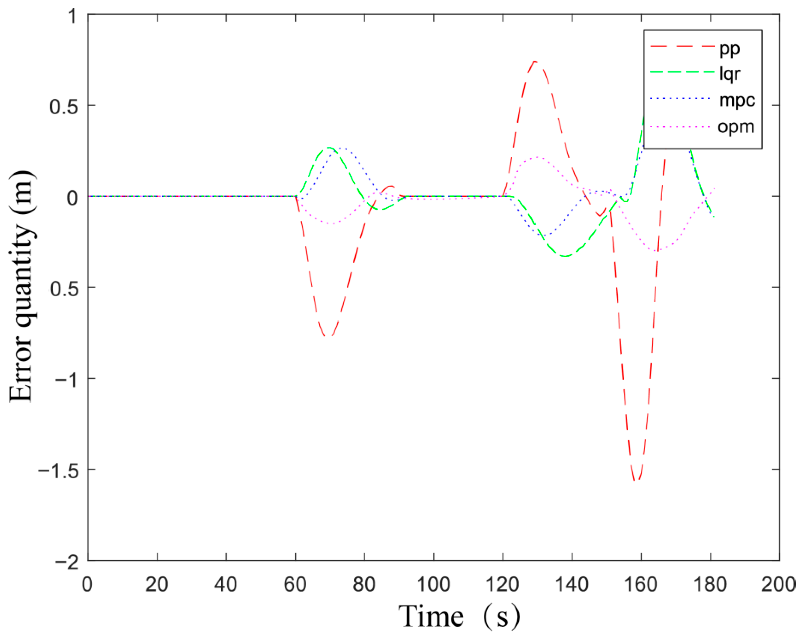
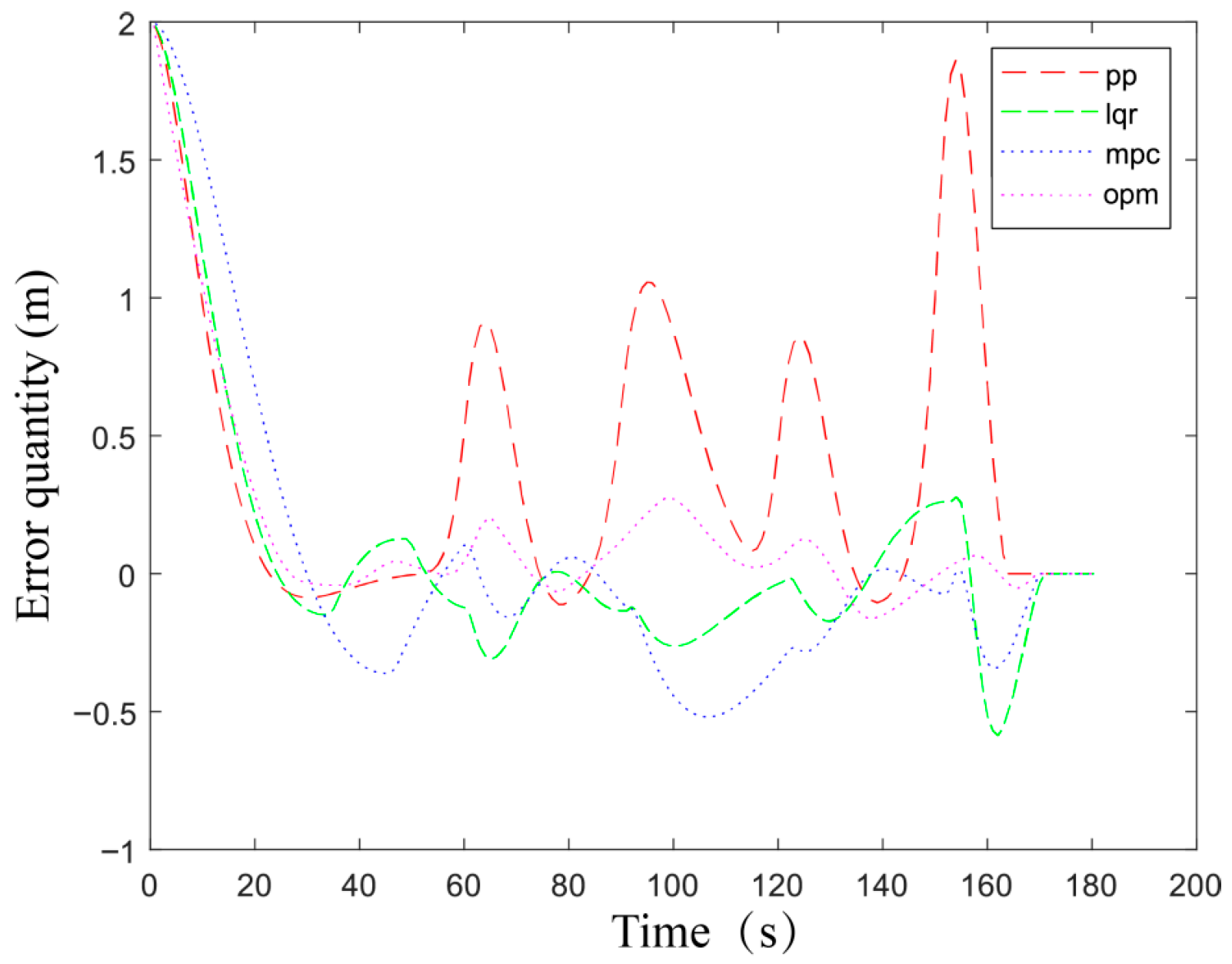
The lateral and longitudinal errors of the main vehicle trajectory are shown in Figure 33 and Figure 34. Compared to the traditional trajectory control algorithm, the optimized algorithm exhibits a maximum lateral error of 0.41 m and a maximum longitudinal error of 0.43 m. Relative to the baseline model, the proposed algorithm reduces lateral and longitudinal errors by an average of approximately 23.4%, with a smoother curve slope. It is evident that the optimized algorithm exhibits minimal deviation from the optimal route without significant disturbances. The trajectory curve generated by the algorithm is smoother and more stable, aligning with vehicle dynamic constraints. Simultaneously, reduced lateral and longitudinal errors significantly increase the vehicle’s clearance relative to lane boundaries and surrounding vehicles. In scenarios such as proximity to lane edges or narrow roads, this enhanced clearance substantially lowers collision risks and improves driving safety. Reduced longitudinal and lateral errors also diminish uncertainty in estimating inter-vehicle distance/relative speed, reducing abrupt braking and acceleration caused by misjudgments and enhancing local traffic flow stability. For overall traffic flow, smaller errors significantly decrease trajectory corrections and lane occupancy time during lane changes and obstacle avoidance, boosting overall traffic efficiency.
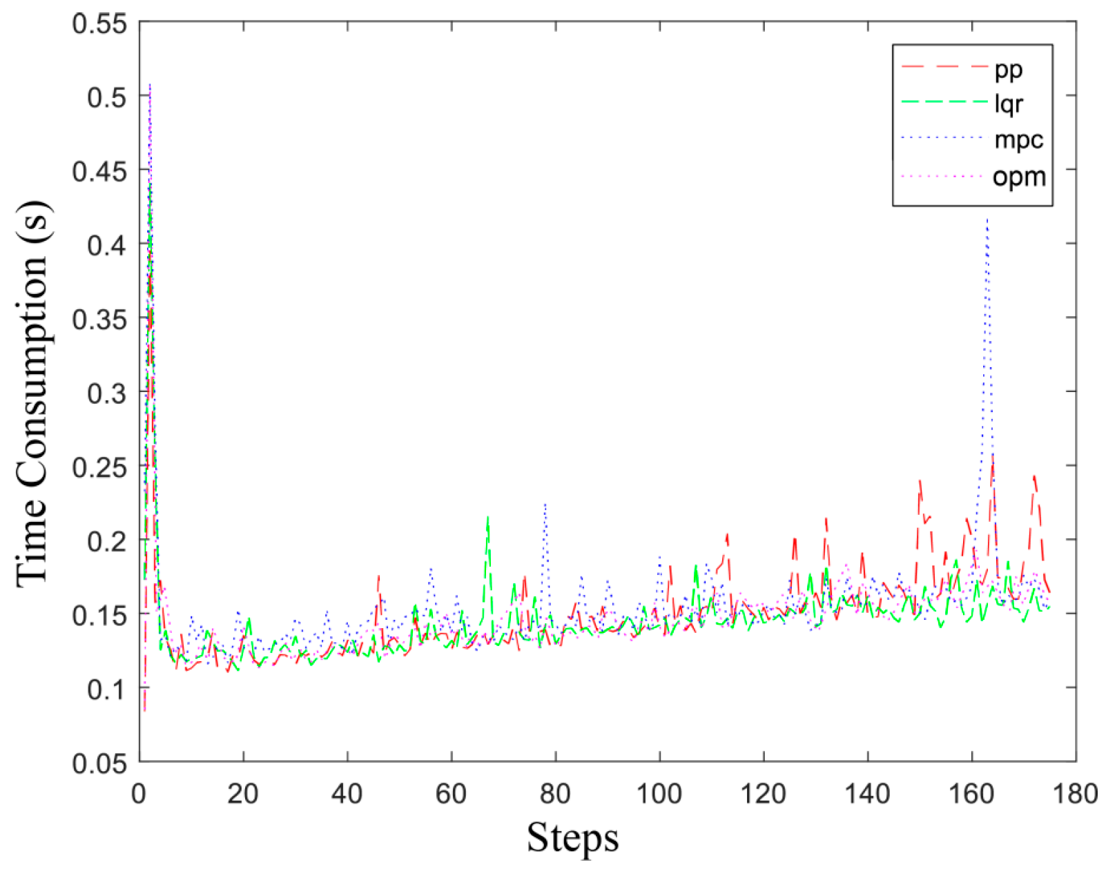
As shown in Figure 35, the algorithm’s computational time demonstrates that while improving trajectory performance and reducing trajectory errors, the processing time does not increase significantly. The per-frame computation time is approximately 0.12 s, aligning with the minimum response time of human drivers.

6. Conclusions

Compared to traditional trajectory control methods for connected autonomous vehicles, the multi-objective trajectory optimization approach based on risk potential fields addresses three key aspects: risk potential fields, vehicle dynamics models, and multi-objective trajectory optimization. It constrains traffic bottleneck zones using driving risk fields to define safe vehicle passage areas and establishes vehicle dynamics models to constrain motion trajectories; nonlinear polynomials are selected to fit the constrained trajectory, and finally, the trajectory is controlled via the SQP algorithm. The optimized method possesses the following characteristics and advantages:
(1) Safety. It establishes a multi-objective driving risk field for CAVs, achieving spatial constraints in road bottleneck areas that consider vehicle-to-vehicle, vehicle-to-road, and human-to-vehicle interactions.
(2) Stability. It constructs a vehicle dynamics model to ensure the stability, safety, and comfort of the selected vehicle trajectory.
(3) Efficiency. Nonlinear polynomial trajectory fitting combined with SQP algorithm control enhances the optimized method’s trajectory fitting accuracy and stability.
Future research may extend the driving risk field theoretical framework to more accurately capture the randomness and highly dynamic characteristics of real traffic environments. Specifically, introducing random disturbance terms into the risk field model can validate its robustness under highly random scenarios in actual traffic. Furthermore, integrating existing cutting-edge research could enable the design of hybrid architecture solutions. By treating the driving risk field as an interpretable safety layer and modeling higher-level random interactions using learning-based or game-theoretic methods, the driving risk field model can be more effectively extended to complex, heterogeneous traffic environments.

Author Contributions

Conceptualization, K.W. and Z.Y.; Methodology, Y.Y.; Software, Z.Y. and Y.Y.; Validation, K.W. and S.C.; Formal analysis, Y.Y.; Investigation, S.C.; Resources, K.W.; Data curation, Z.Y.; Writing—original draft, K.W. and D.Q.; Writing—review and editing, K.W., D.Q. and Z.Y.; Supervision, Y.Y.; Project administration, D.Q.; Funding acquisition, K.W. and D.Q. All authors have read and agreed to the published version of the manuscript.

Funding

This research was funded by the National Natural Science Foundation of China under Grant 52272311 and Grant 51678320 and in part by the Qingdao West Coast New District College President’s Fund under Grant GXXZJJ202301.

Data Availability Statement

The raw data supporting the conclusions of this article will be made available by the authors on request.

Acknowledgments

We are grateful to the anonymous reviewers for their constructive comments that improved the quality of this manuscript. The authors have reviewed and edited the output and take full responsibility for the content of this publication.

Conflicts of Interest

This paper is original and does not contain any content that violates laws and regulations or infringes on the rights of others.

References

  1. Li, X.; Lu, Y.; Zhao, X.; Deng, X.; Xie, Z. Path planning for intelligent vehicles based on improved D* Lite. J. Supercomput. 2024, 80, 1294–1330. [Google Scholar] [CrossRef]
  2. Wang, B.; Ju, D.; Xu, F.; Feng, C. Bi-RRT*: An improved bidirectional RRT* path planner for robot in two-dimensional space. IEEJ Trans. Electr. Electron. Eng. 2023, 18, 1639–1652. [Google Scholar] [CrossRef]
  3. Ding, W.; Zhang, L.; Chen, J.; Shen, S. Safe trajectory generation for complex urban environments using spatio-temporal semantic corridor. IEEE Robot. Autom. Lett. 2019, 4, 2997–3004. [Google Scholar] [CrossRef]
  4. Li, T.; Zhang, L.; Liu, S.; Shen, S. Marc: Multipolicy and risk-aware contingency planning for autonomous driving. IEEE Robot. Autom. Lett. 2023, 8, 6587–6594. [Google Scholar] [CrossRef]
  5. Qie, T.; Wang, W.; Yang, C.; Li, Y.; Zhang, Y.; Liu, W.; Xiang, C. An improved model predictive control-based trajectory planning method for automated driving vehicles under uncertainty environments. IEEE Trans. Intell. Transp. Syst. 2022, 24, 3999–4015. [Google Scholar] [CrossRef]
  6. Borkar, K.K.; Singh, M.K.; Dasari, R.K.; Babbar, A.; Pandey, A.; Jain, U.; Mishra, P. Path planning design for a wheeled robot: A generative artificial intelligence approach. Int. J. Interact. Des. Manuf. 2025, 19, 1315–1326. [Google Scholar] [CrossRef]
  7. Piri, M.; Ash, J.E.; Amani, M.J. Does the Conspicuity of Automated Vehicles with Visible Sensor Stacks Influence the Car-Following Behavior of Human Drivers? A Pilot Study. Transp. Res. Rec. 2025, 2680, 319–335. [Google Scholar] [CrossRef]
  8. Rahmanidehkordi, A.; Ghasemi, A.H. Traffic Density Control for Heterogeneous Highway Systems with Input Con-straints. IEEE Control Syst. Lett. 2024, 8, 2787–2792. [Google Scholar] [CrossRef]
  9. Yang, K.; Liu, L. An improved deep reinforcement learning algorithm for path planning in unmanned driving. IEEE Access 2024, 12, 67935–67944. [Google Scholar] [CrossRef]
  10. Aradi, S. Survey of deep reinforcement learning for motion planning of autonomous vehicles. IEEE Trans. Intell. Transp. Syst. 2020, 23, 740–759. [Google Scholar] [CrossRef]
  11. Liu, X.; Hong, L.; Lin, Y. Vehicle lane change models—A historical review. Appl. Sci. 2023, 13, 12366. [Google Scholar] [CrossRef]
  12. Yan, Y.; Peng, L.; Shen, T.; Wang, J.; Pi, D.; Cao, D.; Yin, G. A multi-vehicle game-theoretic framework for decision making and planning of autonomous vehicles in mixed traffic. IEEE Trans. Intell. Veh. 2023, 8, 4572–4587. [Google Scholar] [CrossRef]
  13. Li, G.; Shi, W. Research on lane-changing decision and control of autonomous vehicles based on game theory. Proc. Inst. Mech. Eng. Part D J. Automob. Eng. 2025, 239, 1566–1576. [Google Scholar] [CrossRef]
  14. Qu, D.; Zhang, K.; Song, H.; Jia, Y.; Dai, S. Analysis and modeling of lane-changing game strategy for autonomous driving vehicles. IEEE Access 2022, 10, 69531–69542. [Google Scholar] [CrossRef]
  15. Qu, D.; Zhao, Z.; Jia, Y.; Wang, T.; Liu, Q. Characterization and modeling of vehicle following dynamics based on Lennard-Jones potential. J. Jilin Univ. (Eng. Ed.) 2022, 52, 2549–2557. [Google Scholar]
  16. Qu, D.; Meng, Y.; Wang, T.; Song, H.; Chen, Y. Car-following Model and Safety Characteristics of Connected Autonomous Vehicle Based on Molecular Force Field. J. Transp. Syst. Eng. Inf. Technol. 2023, 23, 33–41. [Google Scholar]
  17. Wang, B.; Zhang, C.; Ren, S.; Liu, C.; Xie, Z. Expressway driving risk identification method based on velocity risk potential field. J. Zhejiang Univ. (Eng. Sci.) 2023, 57, 997–1008. [Google Scholar]
  18. Jia, Y.F.; Qu, D.Y.; Zhao, Z.X.; Wang, T.; Song, H. Car-following Decision-making and Model for Connected and Autonomous Vehicles Based on Safety Potential Field. J. Transp. Syst. Eng. Inf. Technol. 2022, 22, 85–97. [Google Scholar]
  19. Li, L.; Gan, J.; Ji, X.; Qu, X.; Ran, B. Dynamic Driving Risk Potential Field Model Under the Connected and Automated Vehicles Environment and Its Application in Car-Following Modeling. IEEE Trans. Intell. Transp. Syst. 2020, 99, 122–141. [Google Scholar] [CrossRef]
  20. Liu, P.; Jia, H.; Zhang, L.; Wang, Z. Lane-changing Trajectory Planning for Autonomous Vehicles on Structured Roads. J. Mech. Eng. 2023, 59, 271–281. [Google Scholar]
  21. Wang, J.; Wu, J.; Li, Y. Concept, Principle and Modeling of Driving Risk Field Based on Driver-vehicle-road Interaction. China J. Highw. Transp. 2016, 29, 105–114. [Google Scholar]
  22. Lu, S.; Xie, F.; Zhang, B. Human-Vehicle Cooperative Game Collision Avoidance Based on Asymmetric Potential Fields. Automot. Eng. 2022, 44, 1484–1493. [Google Scholar]
  23. Li, Y.; Li, G.; Peng, K. Research on Obstacle Avoidance Trajectory Planning for Autonomous Vehicles on Structured Roads. World Electr. Veh. J. 2024, 15, 168. [Google Scholar] [CrossRef]
  24. Xu, J.; Yang, K.; Shao, Y.; Lu, G. An experimental study on lateral acceleration of cars in different environments in Sichuan, Southwest China. Discret. Dyn. Nat. Soc. 2015, 2015, 494130. [Google Scholar] [CrossRef]
Figure 1. Technical roadmap of the article.
Mathematics 14 01415 g001
Figure 2. Lane line risk field strength maps.
Mathematics 14 01415 g002
Figure 3. Road Boundary Line Risk Field.
Mathematics 14 01415 g003
Figure 4. Stacked Risk Field Strength Map.
Mathematics 14 01415 g004
Figure 5. Risk potential field distribution map.
Mathematics 14 01415 g005
Figure 6. Schematic representation of risk.
Mathematics 14 01415 g006
Figure 7. Distribution of asymmetric risk potential fields for pedestrians.
Mathematics 14 01415 g007
Figure 8. Schematic diagram of asymmetric risk potential for pedestrians.
Mathematics 14 01415 g008
Figure 9. Vector decomposition of the longitudinal and transverse risk potential fields.
Mathematics 14 01415 g009
Figure 10. Traffic Bottleneck Area Curve Constraints.
Mathematics 14 01415 g010
Figure 11. Vehicle volume calibration.
Mathematics 14 01415 g011
Figure 12. Vehicle corner point constraints.
Mathematics 14 01415 g012
Figure 13. Simulation scenario.
Mathematics 14 01415 g013
Figure 14. Simulated potential field.
Mathematics 14 01415 g014
Figure 15. Movement along the gradient direction.
Mathematics 14 01415 g015
Figure 16. Schematic diagram of the force on the vehicle during lane change.
Mathematics 14 01415 g016
Figure 17. Schematic diagram of velocity potential energy matrix generation.
Mathematics 14 01415 g017
Figure 18. Calibration of optimal angle of incision parameters.
Mathematics 14 01415 g018
Figure 19. Schematic diagram of vehicle trajectory clusters.
Mathematics 14 01415 g019
Figure 20. Nonlinear trajectory fitting via SQP algorithm..
Mathematics 14 01415 g020
Figure 21. Video Data Acquisition Scenario 1.
Mathematics 14 01415 g021
Figure 22. Video Data Acquisition Scenario 2.
Mathematics 14 01415 g022
Figure 23. Video Data Acquisition Scenario 3.
Mathematics 14 01415 g023
Figure 24. Video Data Acquisition Scenario 4.
Mathematics 14 01415 g024
Figure 25. Simulation Scene Construction.
Mathematics 14 01415 g025
Figure 26. Risk potential field quantification.
Mathematics 14 01415 g026
Figure 27. Schematic diagram of trajectory parameter correction.
Mathematics 14 01415 g027
Figure 28. Ablation Experiment 1.
Mathematics 14 01415 g028
Figure 29. Ablation Experiment 2.
Mathematics 14 01415 g029
Figure 30. Angle change under different algorithm controls.

Mathematics 14 01415 g030
Figure 31. Angular slope variation under different algorithmic controls.
Mathematics 14 01415 g031
Figure 32. Comparison of trajectories under different algorithms.
Mathematics 14 01415 g032
Figure 33. Trajectory lateral error with different algorithms.
Mathematics 14 01415 g033
Figure 34. Longitudinal error with different algorithms.
Mathematics 14 01415 g034
Figure 35. Time consumed for different algorithmic trajectories.
Mathematics 14 01415 g035
Table 1. Meaning of Parameters in the Cartesian Coordinate System.
ParameterMeaning
X Lateral coordinate of the vehicle in the Cartesian system
Y Longitudinal coordinate of the vehicle in the Cartesian system
v = d x / d t 2 + d y / d t 2 Speed of the vehicle in the Cartesian system
a = d 2 x / d t 2 2 + d 2 y / d t 2 2 Acceleration of the vehicle in the Cartesian system
θ Heading angle of the vehicle in the Cartesian system
Table 2. Lateral distribution coefficients for different road lanes [15].
Number of LanesDirection of DecreaseRatio of Lateral Distribution Coefficients
Four-lane bidirectionalFrom inner to outer lanes1:0.85
Six-lane bidirectionalFrom inner to outer lanes1:0.9:0.75
Table 3. Relationship between vehicle acceleration and passenger comfort [24].
Vehicle Acceleration (m/s2)Passenger Comfort
a 1.8 High comfort, minimal perception of bumps
1.8 a 3.6 Moderate comfort, bumps noticeable but acceptable
3.6 a Low comfort, strong perception of bumps
Table 4. SQP Computational Data Results.
Vehicle SpeedIteration NumberVariable ChangeComputational CostConstraint ViolationMean CurvatureTrajectory LengthIteration Time
3011.091.099−9.4260.004750.4635.28
22.781.337−8.880
32.121.436−7.937
41.781.150−6.740
52.141.044−5.550
4011.421.113−9.4800.003372.3615.33
23.511.275−8.861
32.631.136−7.945
42.651.215−6.584
52.711.131−4.656
5011.651.126−9.1760.002992.5035.27
23.231.133−7.917
33.481.317−6.692
43.121.236−5.356
53.691.147−5.014
Table 5. Simulation parameters.
ParameterValue
Road potential field A _ r o a d 2
Lane marking parameter A _ l a n e 1
Potential field weight ρ 100
Prediction horizon N p 20
Control horizon N c 5
Simulation step T 0.2
Table 6. Simulation scenario configuration.
Obstructive Vehicle IDLaneLateral Distance to Lead Vehicle (m)Initial Speed (km/h)
CAV122033
CAV214035
CAV316030
CAV429033
Table 7. RMSE validation of different methods.
MethodologiesClustersRMS Average Value (m)RMSE Average
DRF11.7360.9694
20.634
30.985
40.871
50.621
MPC11.8121.048
20.712
30.963
40.921
50.832
PP11.7421.6056
20.754
31.655
41.863
52.014
LQR11.7561.0864
20.814
31.045
40.964
50.853
Table 8. Comparison of p-values for RMSE of different methods.
Validation MethodsMethods of Comparisonp-Value Comparison
Optimization Methods MPC0.393
PP0.0404
LQR0.3454
Disclaimer/Publisher’s Note: The statements, opinions and data contained in all publications are solely those of the individual author(s) and contributor(s) and not of MDPI and/or the editor(s). MDPI and/or the editor(s) disclaim responsibility for any injury to people or property resulting from any ideas, methods, instructions or products referred to in the content.