4.1. Development of the Nonlinear Polynomial Model
Vehicle lane-changing trajectory optimization based on polynomial models typically employs parametric curves to describe trajectories. Compared to traditional autonomous driving trajectory algorithms, this approach offers advantages in intuitiveness, accuracy, and reduced computational complexity. To address the aforementioned requirements for safety, efficiency, and smoothness in lane-changing trajectories, a fifth-degree polynomial-based optimization method is proposed. This approach replaces the spline curve method—which requires multiple segment and node adjustments and may introduce discontinuities at junctions—with a more streamlined solution. Polynomial parameterization provides a compact and continuous representation. This compactness reduces the dimensionality of decision variables and enables efficient integration into the SQP framework. Furthermore, the closed-form derivatives of the polynomial explicitly impose spatial constraints derived from risk field evolution, ensuring both stability and comfort.
The function
is utilized to describe the vehicle’s trajectory, effectively representing the vehicle’s movement from its initial position to its target position. The function governing the vehicle lane-changing trajectory is defined as follows:
where
; denotes the duration of the vehicle lane change;
represents the vehicle’s lateral position in the Cartesian coordinate system;
represents the vehicle’s longitudinal position in the Cartesian coordinate system;
and denote the initial lateral and longitudinal positions of the vehicle in the Cartesian coordinate system, respectively;
, , , and are trajectory adjustment parameters designed to prevent abrupt changes at specific points along the trajectory.
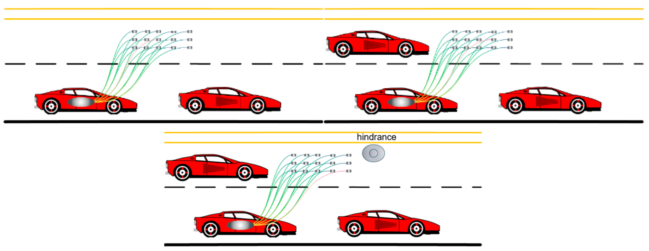
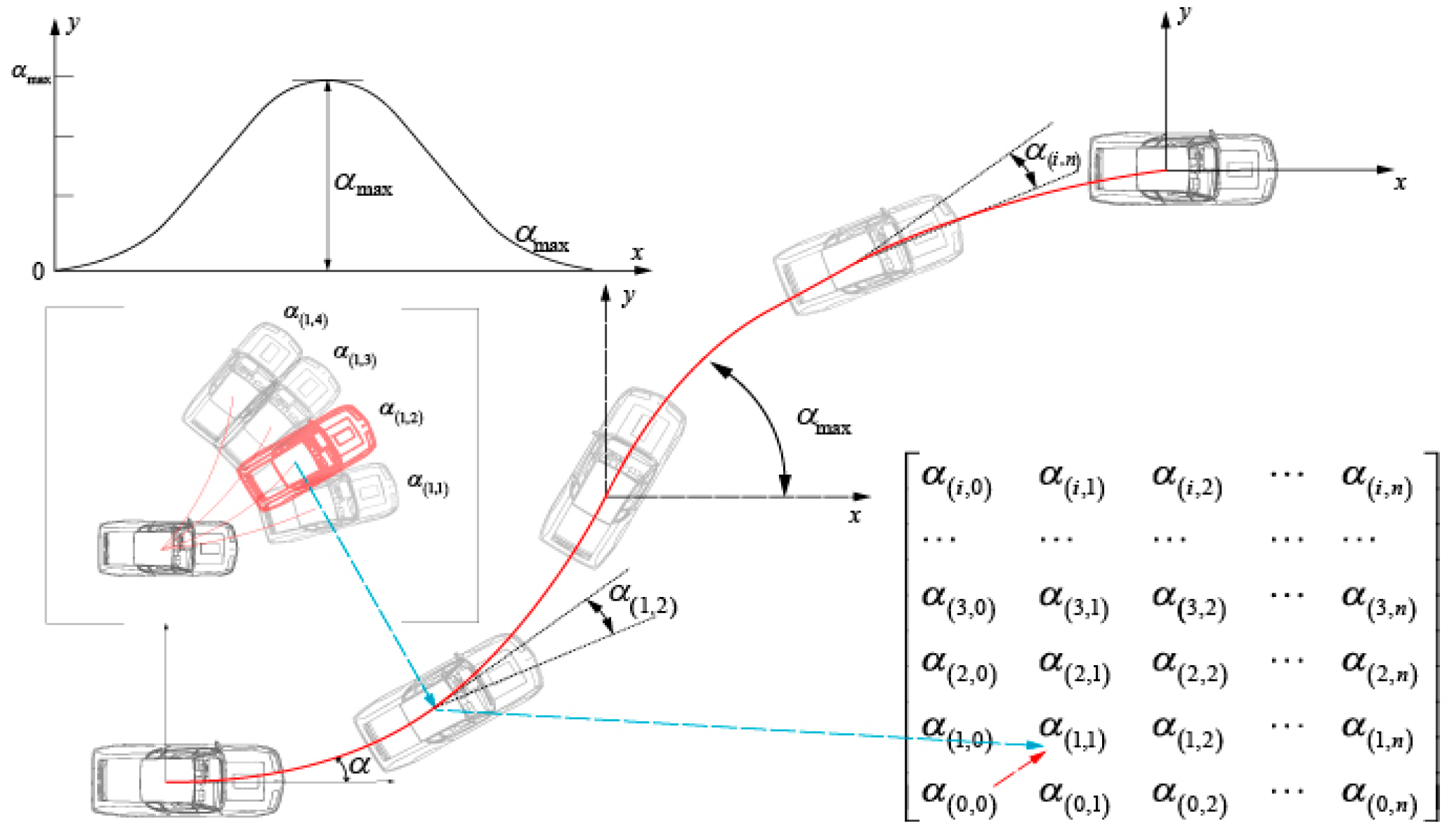
The control of the vehicle lane-changing trajectory primarily involves determining the values of
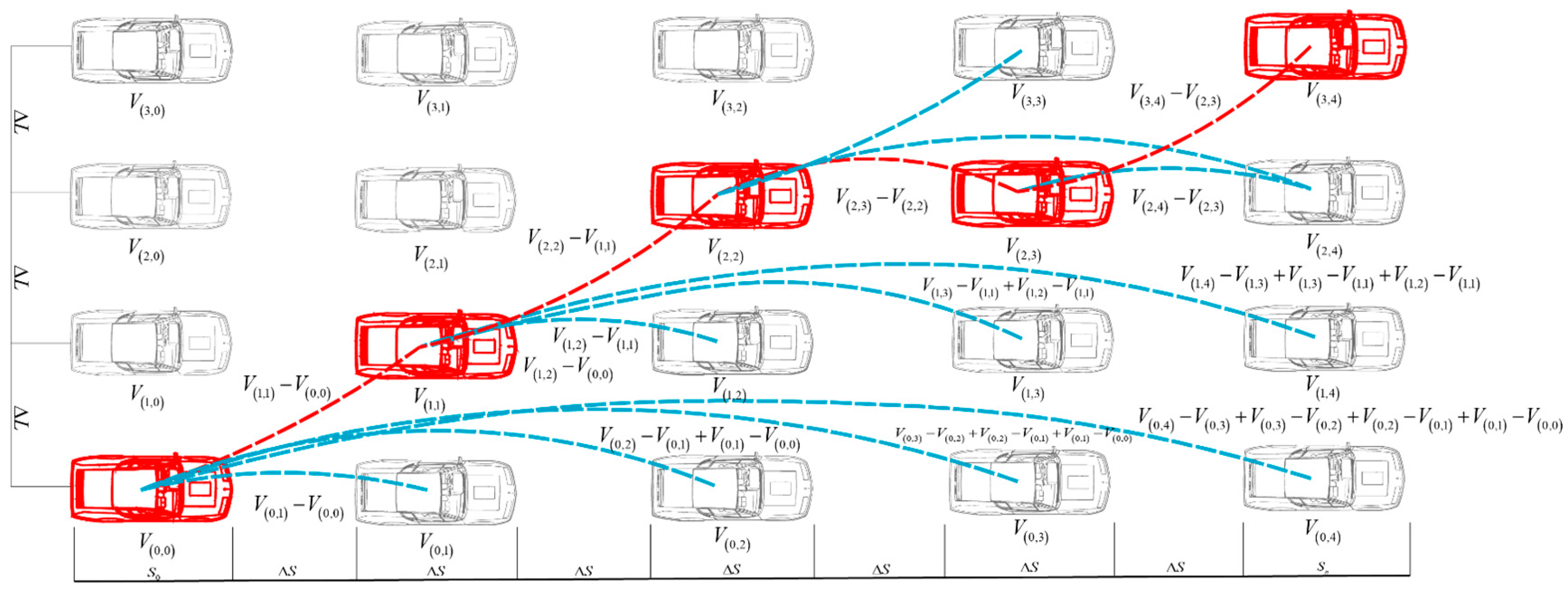
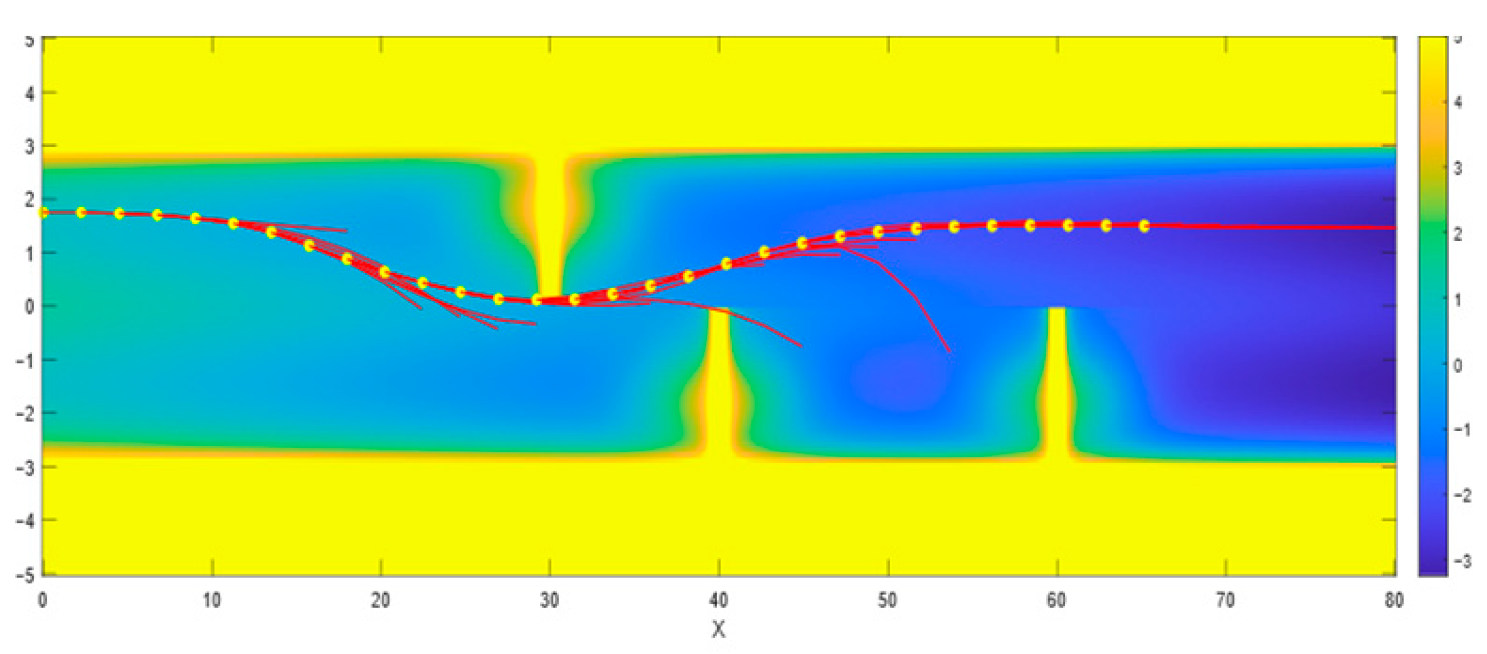
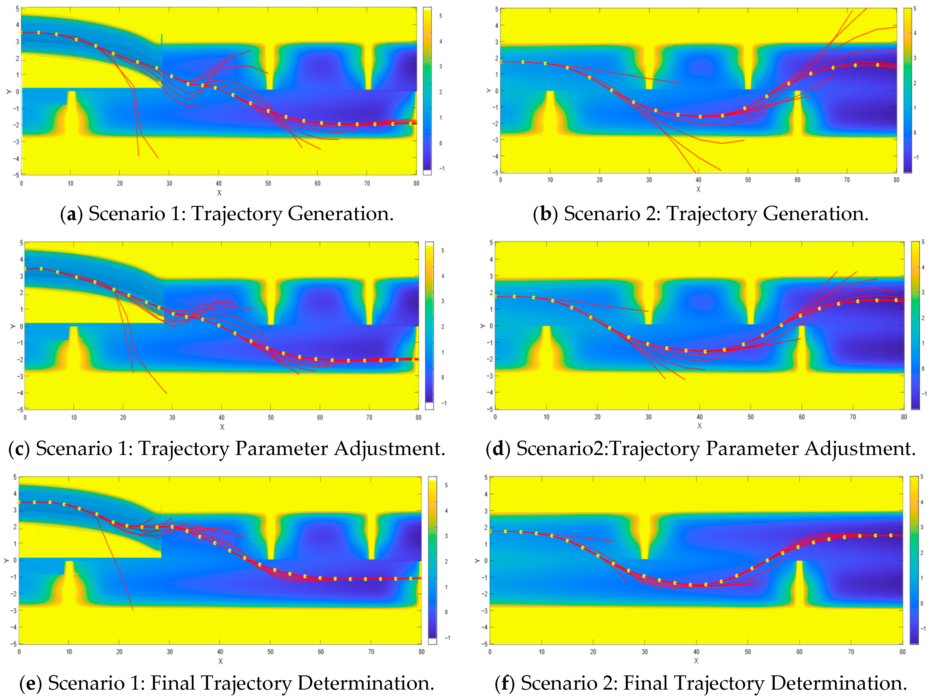
as illustrated in
Figure 19. By imposing constraints on
, multiple clusters of vehicle trajectories can be generated.
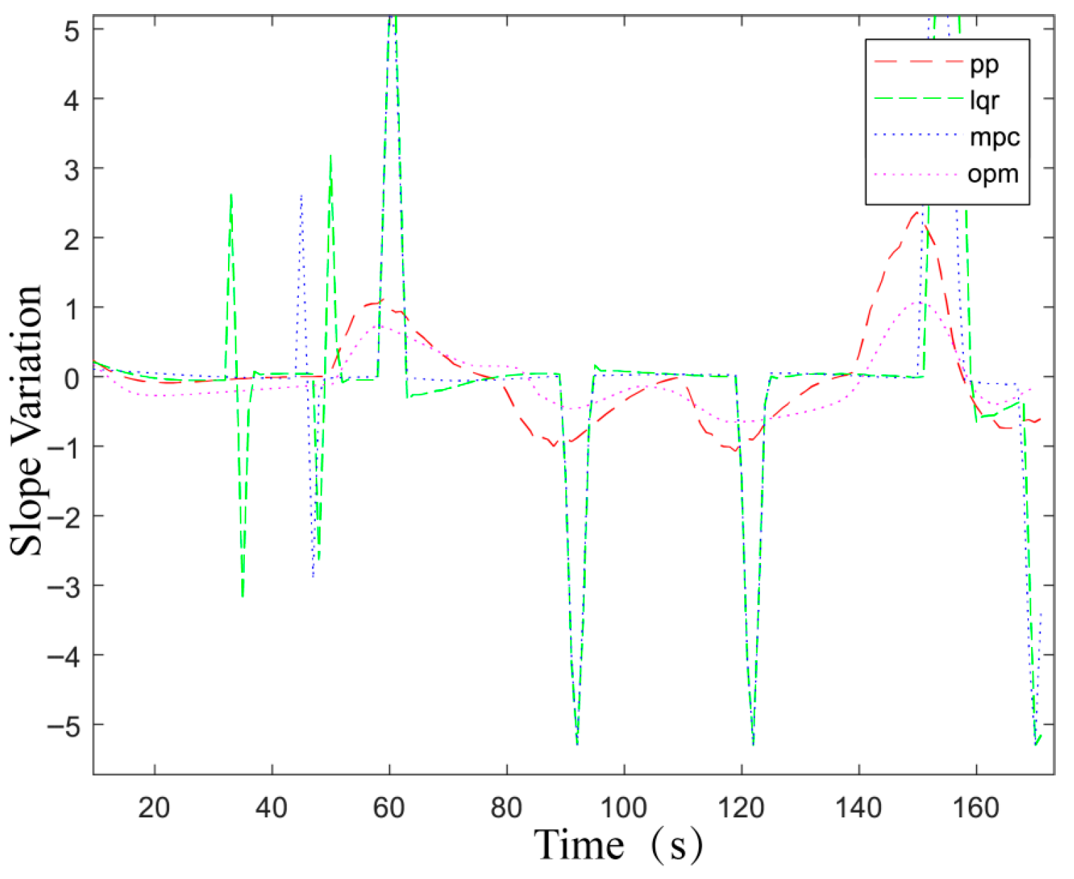
Subsequent to the fitting of vehicle trajectory clusters with polynomial curves, the derivative of the generated fitting curve is computed to ascertain the slope of the curve. The vehicle’s initial and target positions are defined, and three constraint parameters are established. As a result, the fourth derivative of the polynomial curve is calculated, ensuring the fulfillment of the three parameter constraints. This process also guarantees the reasonableness and smoothness of the curve, with the design of vehicle trajectory adjustment parameters aiming to prevent sudden changes in the trajectory derivative, which could yield non-existent trajectory slopes and thus impact the trajectory planning outcome.
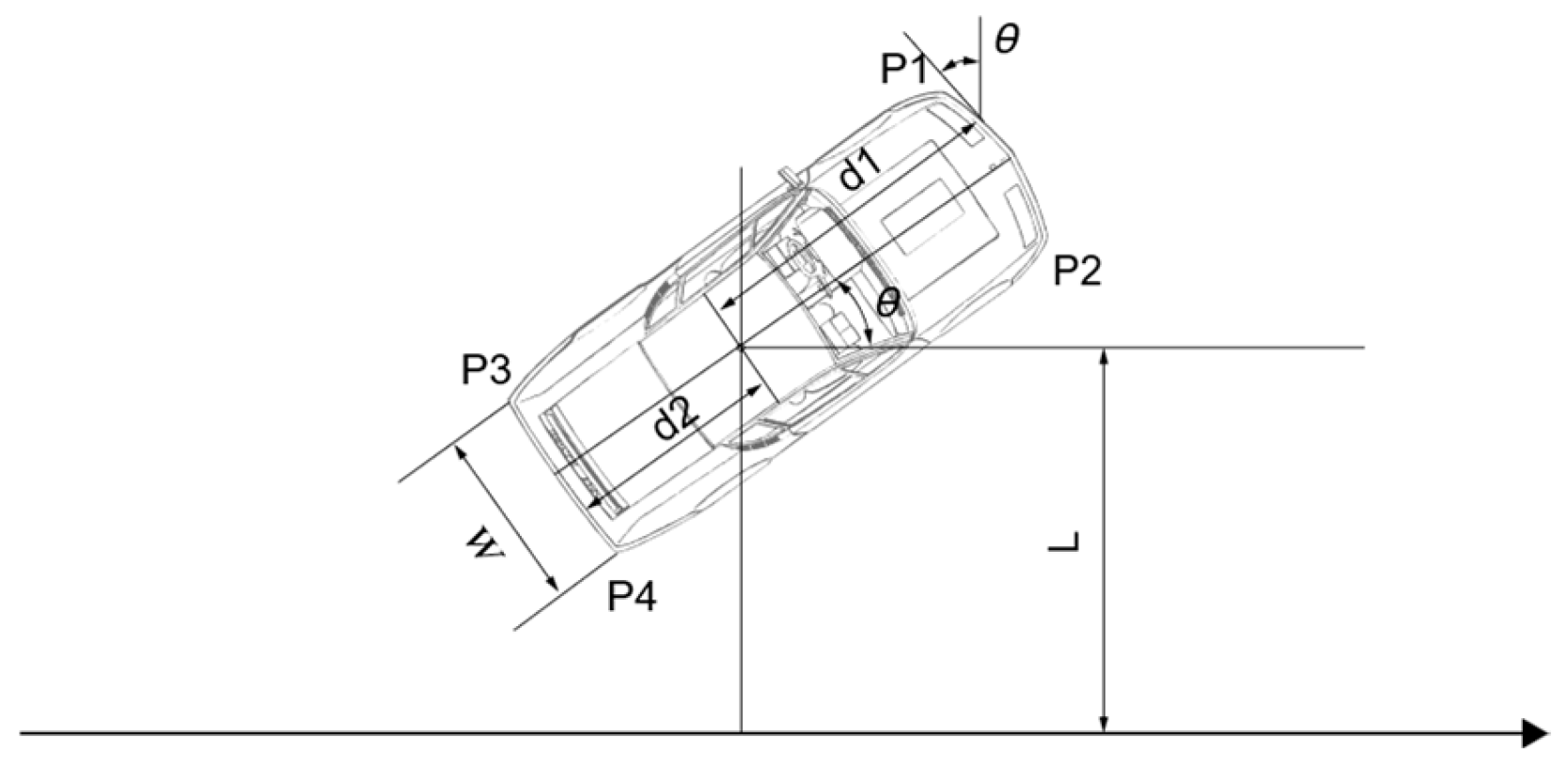
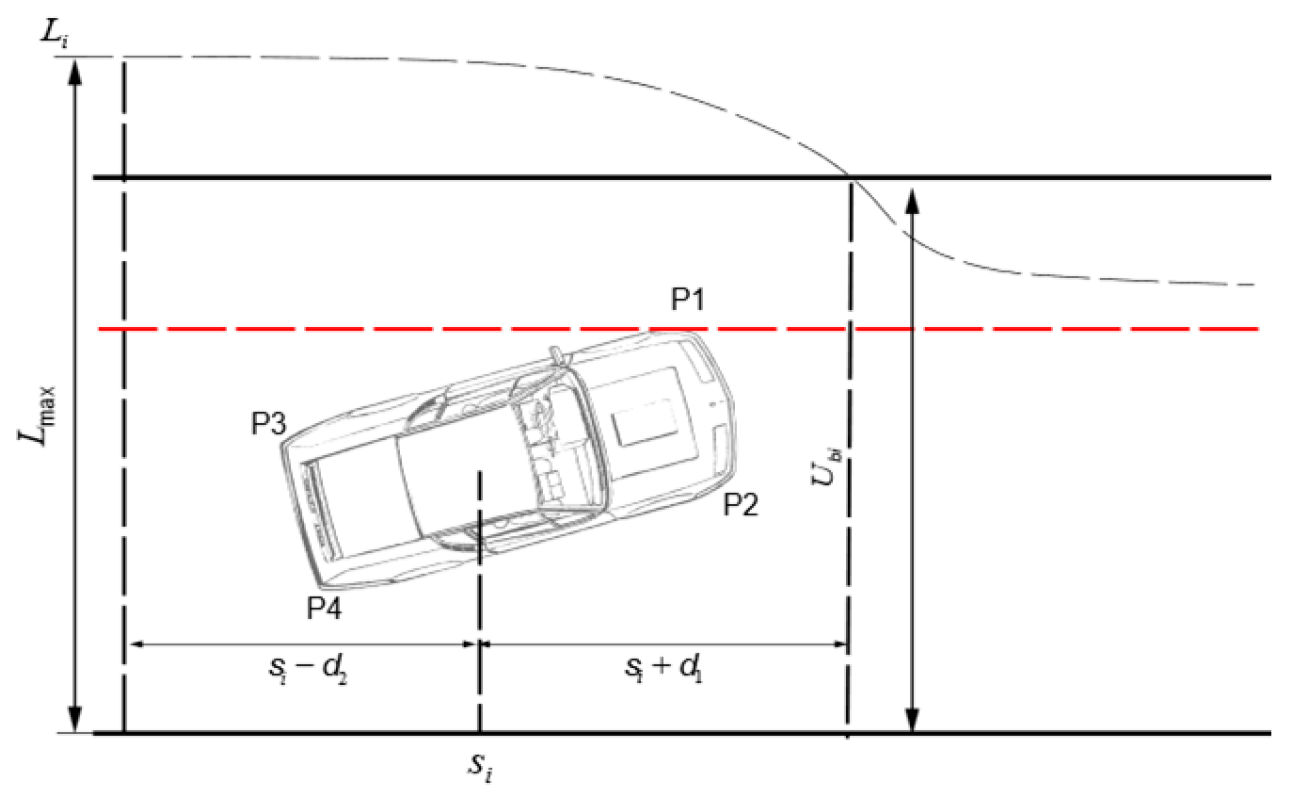
where
,
represent the initial lateral and longitudinal positions of the vehicle, and
,
denote the target lateral and longitudinal positions for the vehicle’s lane change.
The parameters influencing the lane-changing model include and . According to the requirements for the lane-changing trajectory, these parameters must be calibrated as follows:
(1) The vehicle’s heading angle at the initial lane-changing position, , is set to 0, and at the target lane-changing position, , is also set to 0.
(2) The curvature of the vehicle’s trajectory at both the initial and target lane-changing positions is set to zero.
(3) During the lane change, the trajectory generation must comply with the stability parameters, denoted as .
(4) In compliance with national road construction standards, the lateral travel distance within the lane is set at 3.75 m.
Based on the aforementioned formulas and constraints, the unknowns within the trajectory model,
, can be calibrated. The objective function for parameter optimization involving vehicle trajectories is given by the following:
where
represents the differential element of the lane-changing trajectory length, with s being
.
With the above conditions ensured, parameter constraints for the stability of the trajectory are established, where the curvature of the trajectory can be expressed as follows:
where
represents the slope at point
along the curve.
The constraints on trajectory stability are such that under the premises of meeting the specified vehicle trajectory objectives, changes in trajectory curvature should be minimized:
where
is a matrix in the range (0,1); the matrix point value corresponding to the angle that meets the requirements of Equation (35) is 1, and 0 otherwise; and
E is the unit matrix.
After satisfying the two aforementioned equations, a final selection among the remaining clusters of trajectories is conducted based on system throughput efficiency and vehicle passage efficiency:
where
represents the delay in traffic efficiency caused by lane-changing activities of vehicles queuing in the target lane; n denotes the number of vehicles queuing in the target lane.
The objective function described above constitutes a nonlinear programming problem. This study employs Sequential Quadratic Programming (SQP) as its core optimization framework. The trajectory planning task involves nonlinear vehicle dynamics, multi-source risk field constraints, and the synergistic optimization of safety, stability, and comfort. The SQP algorithm transforms the original complex nonlinear optimization problem into a series of subproblems approximated by quadratic programming at each iteration point. By solving the quadratic subproblem to obtain a new solution point, the original problem is then approximated using quadratic programming at this new point. Unlike Model Predictive Control (MPC), which requires repeated optimization at each control step, SQP solves the problem only once per planning cycle, thereby reducing computational cost and enhancing real-time performance. Furthermore, vehicle dynamics constraints and spatial constraints based on driving risk fields can be explicitly incorporated into the SQP optimization process. The specific procedure is as follows:
There exists a constrained nonlinear programming problem of the following form:
where
is the vector to be optimized,
, and for
,
represents inequality constraints and
represents equality constraints.
4.2. Solution of Nonlinear Polynomial Models Using the SQP Method
The SQP algorithm solves subproblems through a quadratic approximation of the Lagrange function:
Here, represents the Lagrange multipliers.
By concurrently linearizing and non-linearizing the constraint conditions, the SQP subproblem related to the original problem can be formulated, with the objective function described as follows:
In this formulation:
represents a global variable;
denotes the gradient; and
is the Hessian matrix of the Lagrange function, approximated using a quasi-Newton method. The constraints of the objective function are as follows:
The solution to the problem is calculated using a semi-definite Newton approximation method, and is represented in the new iterative equation as follows:
Here, is a vector pointing from towards , and is a scalar step size determined during a line search to ensure a sufficient reduction in a specified performance function.
The SQP algorithm is widely acknowledged as a highly effective method for addressing nonlinear optimization problems. In comparison to conventional algorithms, SQP offers numerous merits such as excellent convergence characteristics, superior computational efficiency, and robust capability in boundary searching. Accordingly, this study utilizes the SQP method to optimize trajectory parameters and presents the outcomes of the nonlinear optimization challenge.
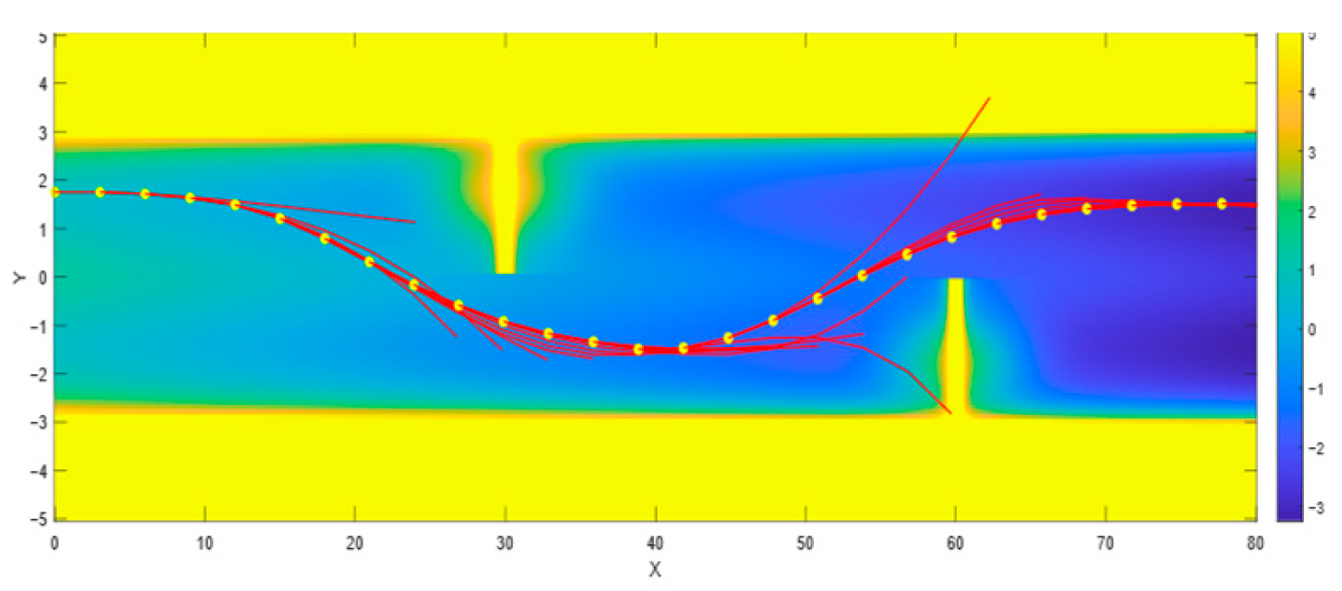
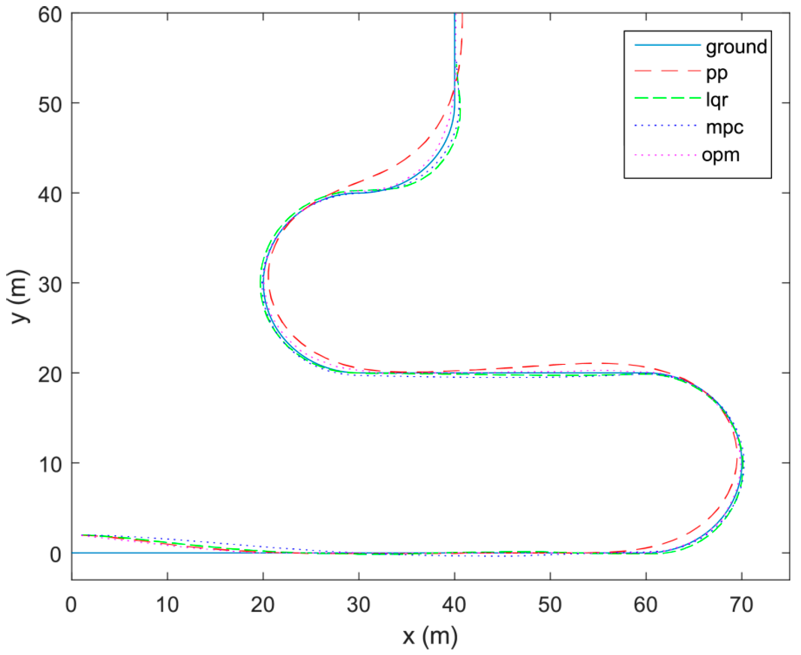
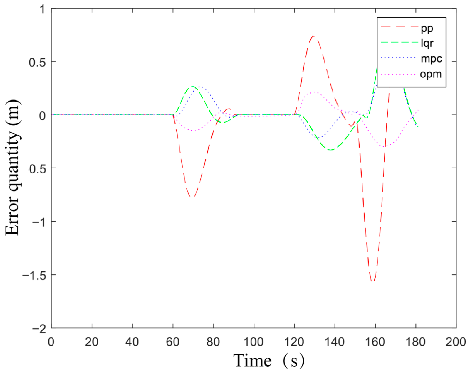
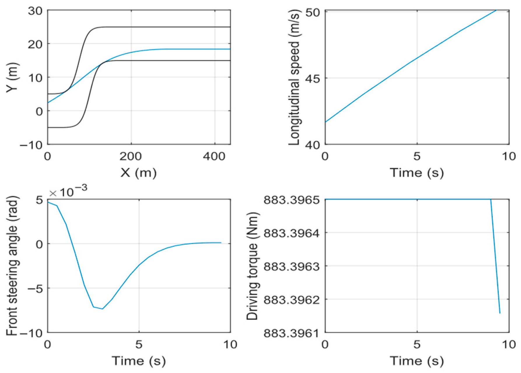
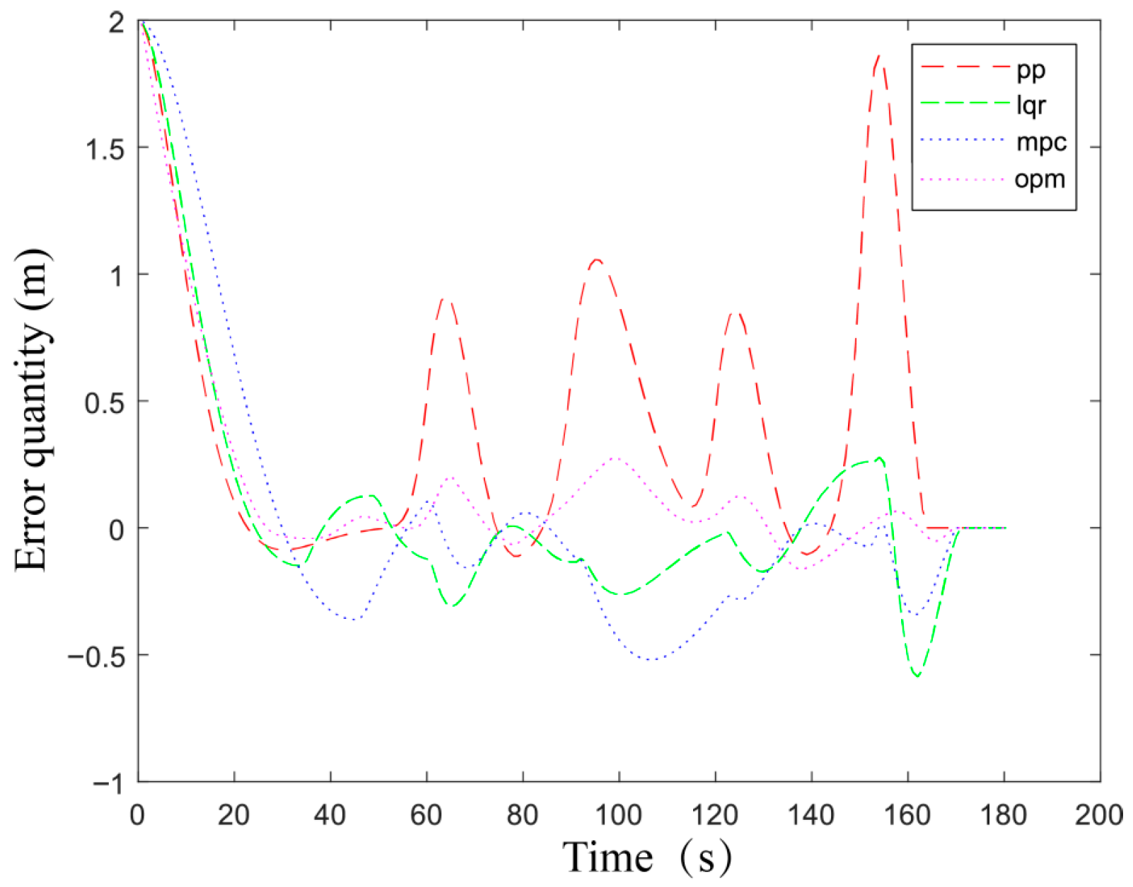
To demonstrate the practicality of the method, the curve-function-fitting vehicle trajectories are solved. To reduce the computation time for trajectory curves while ensuring smoothness and symmetry in lane-change curves, the target curve function is solved by setting and specifying zero acceleration at both the initial and final positions. It should be noted that despite using a simplified quintic polynomial, this approach differs fundamentally from directly employing a cubic polynomial. First, the quintic polynomial possesses six free coefficients, enabling simultaneous satisfaction of position, velocity, and acceleration boundary conditions at both the start and end points of the trajectory. In contrast, the cubic polynomial has only four coefficients, incapable of fully characterizing acceleration boundary constraints. Second, the quintic polynomial explicitly provides an expression for acceleration change rate (acceleration rate), enabling the implementation of comfort constraints related to acceleration changes. Finally, the quintic polynomial is structurally compatible with the Sequential Quadratic Programming (SQP) framework, allowing flexible utilization of higher-order terms for optimization when nonlinear dynamics or safety constraints are present. Lane changes were performed with initial vehicle speeds of 30 km/h, 40 km/h, and 50 km/h. The optimized curve solutions are presented in
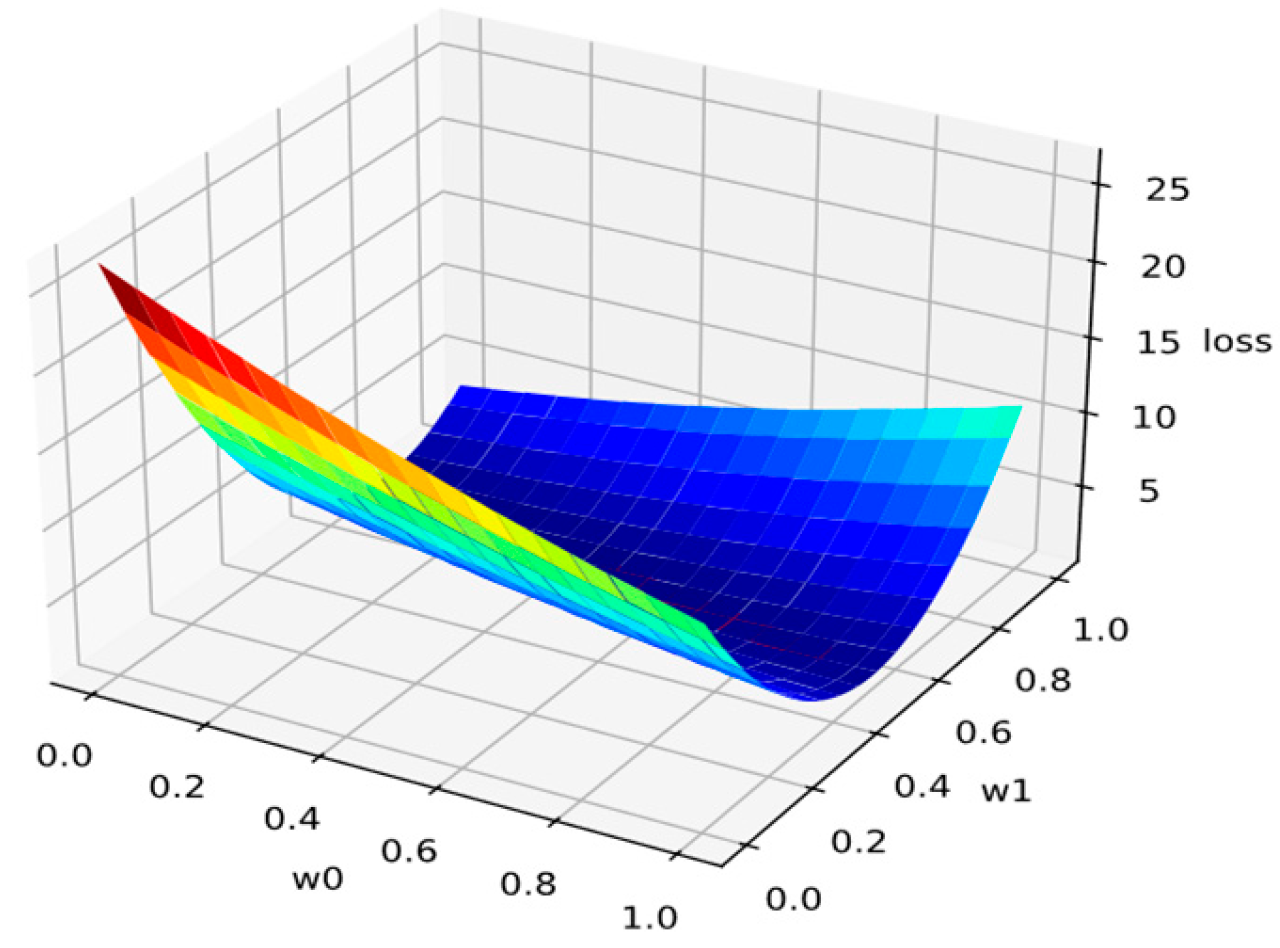
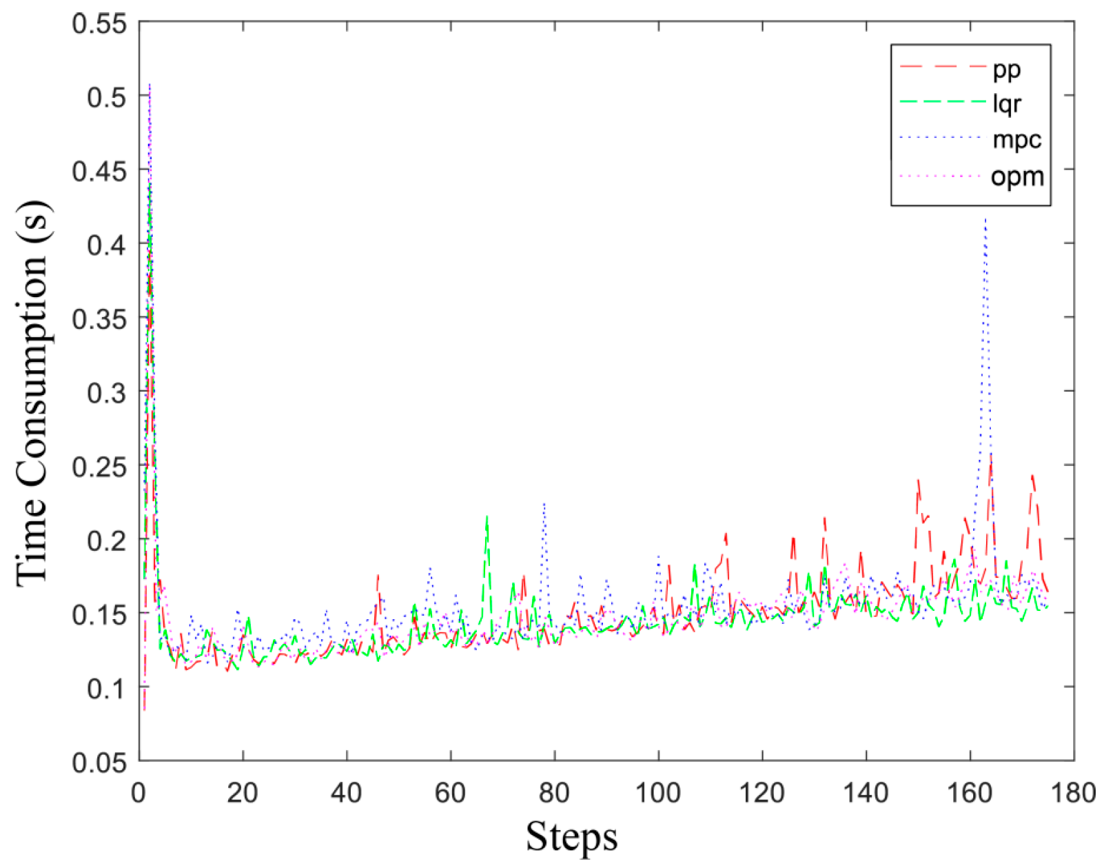
Table 4. As shown in the table, the algorithm achieves an average iteration time of 5.29 s, demonstrating high computational efficiency. While the curve curvature meets stability requirements, the degree of constraint violation gradually decreases with increasing iterations. This indicates that the vehicle trajectory curve progressively approaches a reasonable trajectory curve within the specified range. This is illustrated in
Figure 20.