A Transformer-Based Deep Reinforcement Learning Method for Controller Parameter Modulation in Fault-Tolerant Control

Abstract

This paper proposes a Transformer-based deep reinforcement learning method for adaptive controller parameter modulation. Unlike conventional approaches relying on metaheuristic optimization with fault-specific tuning or model-based gain scheduling, the proposed method learns a unified parameter modulation policy through direct environment interaction without requiring pre-computed optimal solutions. The key innovation lies in a parameter tokenization mechanism that represents each controller parameter as an independent token, enabling self-attention to capture cross-parameter dependencies for coordinated adaptation. A sequential state encoder extracts temporal fault evolution patterns, while fault-aware cross-attention integrates fault context to guide parameter adjustment according to varying fault types and severities. The policy is trained end-to-end using Proximal Policy Optimization with randomized fault injection. Experiments across three systems demonstrate consistent improvements: compared with GA-based tuning, the proposed method achieves lower ISE using a single policy without fault-specific re-optimization; against PSO-based backstepping control, the proposed method achieves tighter error bounds; compared with TD3-based PI scheduling, RMSE is reduced by 55% and recovery time by 47% under time-varying faults. These results validate that the proposed architecture enables effective fault-aware parameter modulation while preserving baseline controller structure.

1. Introduction

Fault-tolerant control (FTC) plays a crucial role in ensuring the safety and reliability of mobile robotic systems operating in uncertain environments. Traditional FTC approaches are primarily model-based, including multiple-model switching and observer-based fault estimation strategies [1,2]. Although these methods are effective when fault characteristics are well understood, their performance strongly depends on the availability of accurate system models and predefined fault patterns.

Recent advances have introduced artificial intelligence techniques into fault diagnosis and recovery. Deep learning approaches such as convolutional neural networks (CNNs) and long short-term memory networks (LSTMs) have demonstrated strong capabilities in temporal fault pattern recognition and data-driven fault isolation [3,4,5,6,7]. These developments have significantly improved the reliability of fault detection and isolation (FDI), providing a solid foundation for subsequent fault recovery and control reconfiguration.

While FDI techniques have reached considerable maturity, restoring system performance after fault occurrence remains a challenging problem. Traditional recovery strategies typically rely on gain scheduling or rule-based parameter adjustment, which are straightforward to implement but lack adaptability under complex or time-varying fault conditions. More advanced model-based methods, including sliding mode control and model predictive control, have been investigated to enhance robustness and recovery capability [8,9,10]. However, their effectiveness often depends on accurate system modeling and careful controller tuning. In parallel, intelligent control techniques such as adaptive neuro-fuzzy inference systems (ANFIS) and neural-network-based controllers have been explored for actuator fault compensation and adaptive control [11,12,13,14]. Although these methods provide flexible control structures, their parameters are typically optimized offline for specific operating conditions, which limits their adaptability to evolving fault scenarios.

Deep reinforcement learning (DRL) has recently emerged as a promising paradigm for adaptive control and fault recovery. Unlike model-based approaches that rely on explicit fault characterization, DRL agents can learn control policies directly through interaction with the environment [15,16,17]. Several studies have demonstrated the effectiveness of DRL in fault-tolerant control of aerial and robotic systems [18]. However, most existing DRL-based FTC approaches employ multilayer perceptron (MLP) policies that struggle to capture long-term temporal dependencies in fault evolution. Recurrent architectures such as RNNs and LSTMs partially address this issue but often suffer from vanishing gradient problems and limited parallelization.

Transformer architectures provide a powerful alternative for modeling sequential and multivariate dependencies through attention mechanisms. By leveraging self-attention, Transformers can capture both long-range temporal correlations and cross-variable interactions while enabling efficient parallel computation. Recent studies have explored Transformer-based controllers for aerial vehicles and adaptive control systems, demonstrating improved adaptability under structural damage or environmental uncertainty [19,20].

Despite these advances, most existing learning-based FTC approaches generate control actions directly, effectively replacing the baseline controller. Although such end-to-end control strategies offer flexibility, they may compromise interpretability, safety guarantees, and certification compatibility provided by well-established control architectures [21]. In safety-critical applications, maintaining a stable baseline controller while adaptively tuning its parameters is often a more practical strategy.

Controller parameter modulation provides a promising pathway for achieving adaptive fault recovery while preserving the structure of conventional control systems. By dynamically adjusting controller gains and internal parameters, system performance degradation caused by faults can be mitigated without replacing the underlying control architecture [22,23,24]. However, classical approaches such as gain scheduling and metaheuristic optimization typically require fault-specific re-optimization and struggle to handle nonlinear coupling between controller parameters [25].

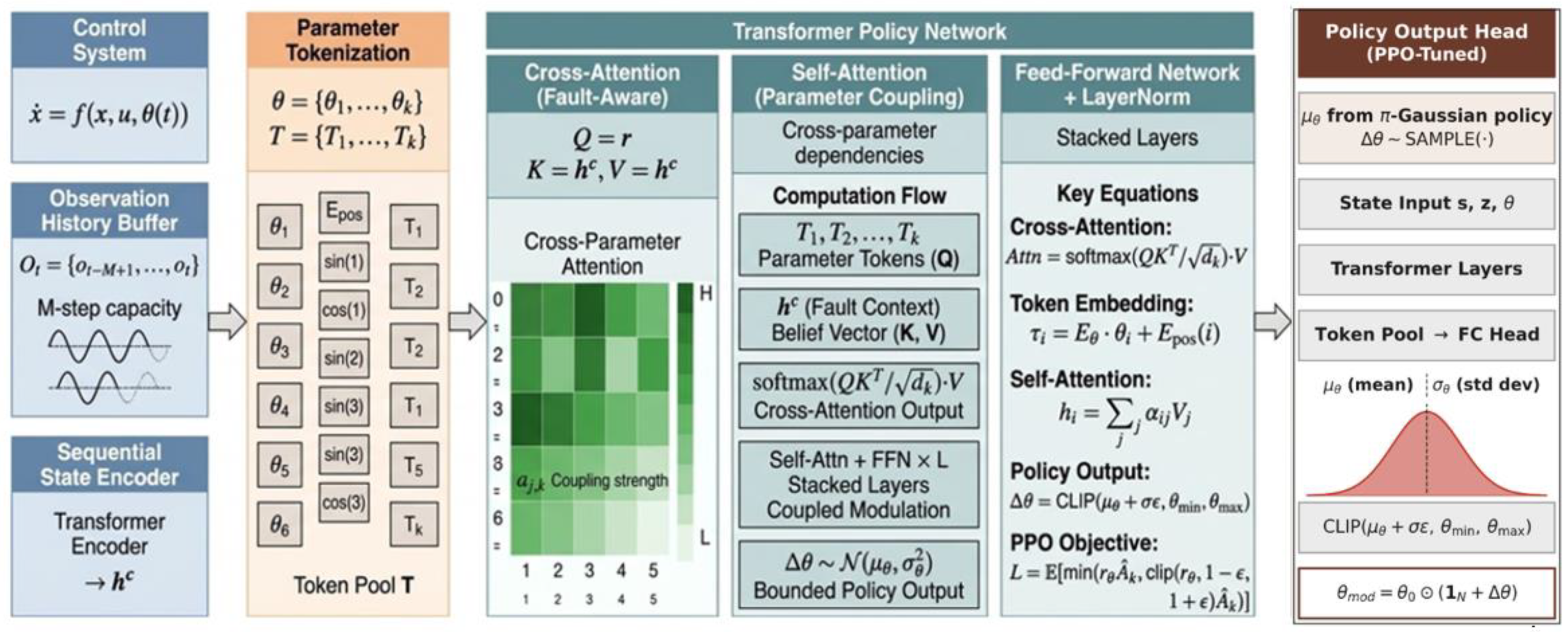
Motivated by these challenges, this paper proposes a Transformer-guided deep reinforcement learning framework for adaptive controller parameter modulation in fault recovery. The proposed method maintains the baseline controller structure while learning a policy that adjusts controller parameters according to system observations and fault conditions. Figure 1 illustrates the overall architecture of the proposed method. The left block represents the Control System and Observation History Buffer, which store the M most recent state-fault estimate pairs O_t. The Parameter Tokenization block converts each nominal controller parameter ${\theta }_i$ into a token T_i combined with positional embedding E_pos, forming the Token Pool T. The central Transformer Policy Network processes these tokens through Cross-Attention (Fault-Aware), which uses fault context h^c as Key and Value; Self-Attention (Parameter Coupling), which captures cross-parameter dependencies via coupling strength ${\alpha }_{j,k}$; and a Feed-Forward Network. The right Policy Output Head samples modulation $\Delta \theta$ from a Gaussian policy parameterized by mean ${\mu }_{\theta }$ and standard deviation ${\sigma }_{\theta }$, and applies the bounded update ${\theta }_{mod}={\theta }_0\odot (1_N+\Delta \theta )$.

The main contributions of this work are summarized as follows:

(1)

Transformer-guided parameter modulation framework. A deep reinforcement learning framework is proposed for adaptive controller parameter modulation, enabling online fault recovery without replacing the baseline controller structure.

(2)

Parameter tokenization and attention-based coupling modeling. Controller parameters are represented as token embeddings and processed using a Transformer policy network, allowing self-attention mechanisms to capture cross-parameter dependencies and coordinate parameter adaptation.

(3)

Fault-aware cross-attention mechanism for adaptive recovery. A cross-attention mechanism is introduced to incorporate fault type and severity information into the policy network, enabling context-aware parameter adjustment under diverse fault conditions.

(4)

Temporal belief representation for fault evolution modeling. A sequential state encoder is designed to extract temporal patterns from historical system observations, allowing the controller to anticipate fault evolution and perform proactive parameter adaptation.

2. Problem Formulations

2.1. System Modeling and Adaptive Parameter Modulation

Consider a general nonlinear dynamical system operating under system faults, anomalies, and performance-degrading conditions, modeling uncertainties and external disturbances. The system dynamics are described by

$$\dot{x}\left(t\right)=f\left(x\left(t\right),u\left(t\right),{\varphi }_a\left(t\right)\right)$$

(1)

where $x\left(t\right)\in {\mathbb{R}}^n$ denotes the system state, $u\left(t\right)\in {\mathbb{R}}^m$ is the control input, and ${\varphi }_a\left(t\right)\in {\mathbb{R}}^{n_f}$ represents a generalized degradation vector capturing the type, location, severity, or evolution of system performance loss.

A baseline controller with adjustable parameters generates control commands according to:

$$u\left(t\right)=C\left(x\left(t\right),x_{ref}(t),{\theta }_0\right)$$

(2)

where $x_{ref}(t)$ is the reference trajectory, $C(\cdot )$ denotes a parameterized control law such as PID control, fuzzy control, or neural-network-based controllers, and ${\theta }_0\in {\mathbb{R}}^N$ denotes the nominal controller parameters designed to achieve satisfactory closed-loop performance under fault-free conditions, with N being the total number of adjustable parameters. However, when faults or degradations occur, the nominal parameter set becomes suboptimal, leading to degraded tracking accuracy, increased control effort, or even instability.

The objective of this work is to learn an adaptive parameter modulation policy that dynamically adjusts controller parameters in response to observed system behavior and degradation information:

$$\Delta \theta \left(t\right)={\pi }_{\varphi }\left(s\left(t\right)\right)$$

(3)

where ${\pi }_{\varphi }(\cdot )$ denotes the learned policy network parameterized by weights $\varphi$, and $s\left(t\right)=\left(h_c\right(t),{\theta }_0)$ is the policy input state comprising the belief representation $h_c(t)\in {\mathbb{R}}^d$ extracted from observation history by the sequential state encoder (Section 3.1), and the nominal parameter vector ${\theta }_0$. The output $\Delta \theta \left(t\right)\in [-ϵ,ϵ{]}^N$ is the bounded parameter modulation vector, where N denotes the total number of adjustable controller parameters, so that ${\theta }_0,\Delta \theta \left(t\right)\in {\mathbb{R}}^N$.

$${\theta }^{\prime }\left(t\right)={\theta }_0\odot \left(1_N+\Delta \theta \left(t\right)\right)$$

(4)

Here $1_N\in {\mathbb{R}}^N$ denotes the all-ones vector of dimension N, and $\odot$ denotes the Hadamard (element-wise) product. This formulation ensures that each parameter is scaled independently by its corresponding modulation factor $\left(1+\Delta {\theta }_i\left(t\right)\right)$, preserving the physical units and sign of each parameter. The bound $ϵ>0$ is a scalar hyperparameter defining the trust region of parameter modulation. It is selected empirically via grid search to balance recovery aggressiveness against closed-loop stability margins, and is treated as fixed throughout training and deployment. The resulting modulated control input is given by

$$u\left(t\right)=C\left(x\left(t\right),x_{ref}\left(t\right),{\theta }^{\prime }\left(t\right)\right)$$

(5)

Remark 1. 

The control law (5) assumes availability of the full state vector $x\left(t\right)$ for feedback. In the considered experimental platforms—quadrotor UAVs, transformable quadrotors, and DC motor systems—the full state comprising position, velocity, and attitude can be obtained through standard onboard sensor fusion (IMU, encoders, optical flow), which is standard practice in robotics and motion control. Accordingly, the full state feedback assumption is practically justified for the target application class. Extension to partial-observation settings, where only an output $y\left(t\right)=h\left(x\right(t\left)\right)$ is available, can be addressed by replacing $x\left(t\right)$ in (5) with a state estimate $\widehat{x}(t)$ from a Luenberger observer or extended Kalman filter, which is left as future work.

Accordingly, the closed-loop dynamics under the proposed framework can be expressed as:

$$\dot{x}\left(t\right)=f(x\left(t\right),C\left(x\left(t\right),x_{ref}\left(t\right),{\theta }_0\odot \left(1_N+{\pi }_{\varphi }\left(s\left(t\right)\right)\right)\right),{\varphi }_a\left(t\right))$$

(6)

2.2. Optimization Model

The design variable is the parameter modulation vector $\Delta \theta \left(t\right)\in [-ϵ,ϵ{]}^N$, representing real-time adjustments to the nominal controller parameters ${\theta }_0$, where N is the number of adjustable parameters. The objective is to minimize the cumulative tracking error $e(t)=x(t)-x_{ref}(t)$ over the recovery horizon $\left[t_f,t_f+T_r\right]$ following fault onset at t_f. Here ${\varphi }_a(t)\in {\mathbb{R}}^{n_f}$ is the generalized degradation vector introduced in (1), capturing fault type, location and severity. Three regularization terms are additionally incorporated to penalize excessive control effort and large parameter excursions, weighted by coefficients $a_1,a_2,a_3>0$. A fourth term $-a_4\cdot {\mathcal{R}}_{rec}$ is included as a recovery bonus, where ${\mathcal{R}}_{rec}$ measures the duration for which $\parallel e\left(t\right)\parallel <{ϵ}_r$ is sustained within the recovery horizon, explicitly incentivizing rapid and stable fault recovery beyond mere error minimization. Therefore, the optimization problem is formulated as:

$$\underset{\Delta \theta }{\mathrm{m}\mathrm{i}\mathrm{n}}J=a_1{\int }_{t_f}^{t_f+T_r}{‖e\left(t\right)‖}^{2}dt+a_2{\int }_{t_f}^{t_f+T_r}{‖u\left(t\right)‖}^{2}dt+a_3{\int }_{t_f}^{t_f+T_r}{‖\Delta \theta \left(t\right)‖}^{2}dt-a_4{\mathcal{R}}_{rec}$$

(7)

$$s.t.\mathrm{ }\mathrm{ }\mathrm{ }\mathrm{ }C1:\dot{x}(t)=f(x(t),C\left(x(t),x_{ref}(t),{\theta }_0\odot \left(1_N+{\pi }_{\varphi }\left(s\left(t\right)\right)\right)\right),{\varphi }_a(t)),\mathrm{ }\mathrm{ }\mathrm{ }\forall t\in \left[t_f,\mathrm{ }{t}_f+T_r\right]$$

$$C2:a_t=\Delta {\theta }_t\in {\left[-ϵ,ϵ\right]}^N, \forall t\in \left[t_f,t_f+T_r\right]$$

The optimization problem in (7) is solved via deep reinforcement learning rather than classical optimization, as $f(\cdot )$ is nonlinear and ${\varphi }_a(t)$ is only partially observable. The cumulative tracking error is minimized indirectly through the design of the instantaneous reward signal r_t in (27), which serves as the discrete-time surrogate for the continuous-time objective J. Specifically, the term $-a_1\parallel e\left(t\right){\parallel }^2$ directly penalizes tracking deviation at each timestep, incentivizing the policy to reduce e(t) continuously throughout the recovery horizon $\left[t_f,t_f+T_r\right]$. The term $-a_2\parallel u\left(t\right){\parallel }^2$ penalizes excessive control effort to prevent aggressive compensation that may destabilize the system, while $-a_3\parallel \Delta {\theta }_t{\parallel }^2$ discourages unnecessary parameter excursions away from the nominal design. The recovery bonus $+a_4\cdot 1_{recovered}$ provides an explicit incentive for the policy to achieve and sustain tracking error below the threshold ${ϵ}_r$, directly targeting the recovery objective J_rec in (26). At each timestep, the PPO algorithm updates the policy ${\pi }_{\varphi }$ to maximize the expected cumulative reward $\mathbb{E}\left[{\sum }_t{\gamma }^t{r}_t\right]$, ** which serves as a surrogate objective aligned with minimizing the cumulative tracking error J over the recovery horizon while satisfying constraints C1 and C2.

Remark 2. 

In the ideal case of perfect tracking where $x(t)\equiv x_{ref}(t)$, the first term vanishes since $e\left(t\right)\equiv 0$. However, the control input $u\left(t\right)$ is not necessarily zero: in the fault-tolerant control setting considered here, maintaining $x(t)=x_{ref}(t)$ against persistent fault-induced disturbances inherently requires sustained control effort. Similarly, $\Delta \theta \left(t\right)$ generally does not vanish under persistent faults, as the modulation policy must continuously counteract the fault effect to maintain tracking, so that ${\theta }^{\prime }(t)\ne {\theta }_0$ even at steady state. The regularization terms $a_2\parallel u\left(t\right){\parallel }^2$ and $a_3\parallel \Delta \theta \left(t\right){\parallel }^2$ penalize excessive control energy and unnecessary parameter drift, respectively, ensuring well-posedness of the optimization problem and avoiding degenerate policies. In the discrete-time reinforcement learning implementation, the recovery objective is realized as an indicator-based reward $a_4\cdot 1_{recovered}$, which is equivalent to the continuous-time formulation up to a sign convention.

Constraint C1, given by Equation (6), enforces the complete closed-loop dynamics under the proposed modulation framework, ensuring that system evolution is always governed by the modulated controller within the recovery horizon $\left[t_f,t_f+T_r\right]$. Constraint C2 restricts the modulation vector to the bounded region $\left[-ϵ,ϵ{]}^N\right.$, preserving stability margins and maintaining proximity to the nominal controller design. The weighting coefficients $a_1,a_2,a_3,a_4>0$ are treated as hyperparameters and determined via grid search. Since $f(\cdot )$ is nonlinear and ${\varphi }_a(t)$ is only partially observable, this problem is intractable by classical optimization methods. To address this, the problem is solved via deep reinforcement learning, which learns an adaptive modulation policy through direct environment interaction without requiring explicit system models or fault-specific re-optimization, as detailed in Section 3.

3. Methodology

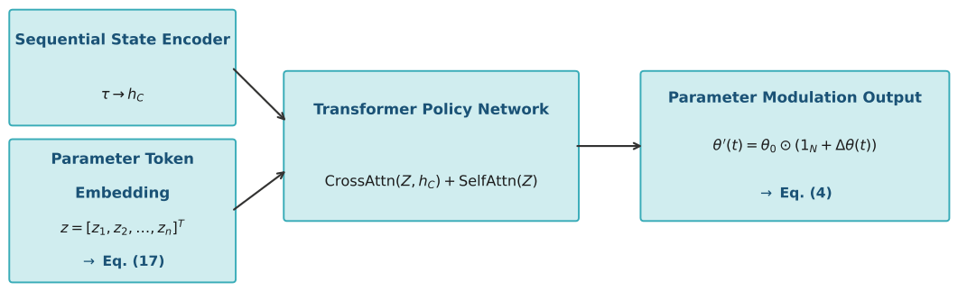
To solve the optimization problem formulated in Section 2, this paper proposes a Transformer-based deep reinforcement learning method that learns an adaptive parameter modulation policy through direct interaction with the fault-affected environment. The proposed method consists of four modules: Sequential State Encoder, Parameter Token Embedding, Transformer Policy Network, and Parameter Modulation Output. At each timestep, the sequential encoder processes observation history to extract belief state h_c. Then controller parameters are embedded as token representations and the Transformer policy models cross-parameter dependencies through self-attention and integrates fault context through cross-attention. After then, bounded modulation values are output to adjust the controller. Figure 2 shows the three-module pipeline. The Sequential State Encoder takes observation history $\mathcal{T}$ and produces belief vector $h_c\in {\mathbb{R}}^d$. The Parameter Token Embedding maps ${\theta }_0$ to token sequence $z=[z_1,\dots ,z_n{]}^T\in {\mathbb{R}}^{N\times d}$. Both are fed to the Transformer Policy Network, which applies $\mathrm{CrossAttn}(Z,h_c)+\mathrm{SelfAttn}\left(Z\right)$ and outputs modulation via ${\theta }^{\prime }(t)={\theta }_0\odot (1_N+\Delta \theta (t))$.

3.1. Sequential State Encoder

In practical systems, fault or degradation variables $\varphi \left(t\right)$ are generally not directly observable. Instead, only noisy and delayed estimates $\widehat{\varphi }\left(t\right)$ may be available from monitoring, diagnosis, or estimation modules. Fault estimation is subject to two fundamental limitations. First, diagnostic algorithms introduce a latency T > 0 due to the finite time required for data acquisition and fault isolation, so the most recent available estimate reflects the fault state at time t − T rather than the current instant. Second, estimation algorithms introduce stochastic noise $\xi \left(t\right)$ due to sensor imperfections and model mismatch. Consequently, the available fault estimate is modeled as:

$${\widehat{\varphi }}_a\left(t\right)=\xi \left(t\right)+{\varphi }_a\left(t-T\right)$$

(8)

where T > 0 denotes the estimation latency and $\xi \left(t\right)$ is zero-mean estimation noise. This model motivates the use of a history-based belief representation rather than instantaneous fault observation. Moreover, degradation processes often exhibit nonstationary and time-varying behavior:

$${\dot{\varphi }}_a\left(t\right)=g\left({\varphi }_a\left(t\right),t\right)$$

(9)

which cannot be inferred reliably from instantaneous observations alone. As a result, the decision-making problem cannot be accurately modeled as a fully observable Markov Decision Process (MDP). To address this challenge, the control adaptation problem is formulated as a Partially Observable Markov Decision Process (POMDP), where the decision states depend on a history of observations:

$$O_{t-M+1:t}=\left\{{(x}_{t-M+1},{\widehat{\varphi }}_{a,t-M+1}),\dots ,{(x}_t,{\widehat{\varphi }}_{a,t})\right\}$$

(10)

A sequential encoder is employed to extract a latent belief representation $h_c\left(t\right)$ from observation history, which serves as a sufficient statistic for decision making. This transforms the original POMDP into an approximate MDP in the belief space, providing a principled justification for temporal modeling.

Given observation history $\left\{(x_{t-M+1},{\widehat{\varphi }}_{a,t-M+1}),\dots ,(x_t,{\widehat{\varphi }}_{a,t})\right\}$, each observation is embedded:

$${\mathrm{e}}_{\mathrm{i}}=W_e\left[x_{\mathrm{i}};{\widehat{\varphi }}_{a,i}\right]+b_e e_i\mathit{\in }{\mathbb{R}}^d$$

(11)

where $W_e\in {\mathbb{R}}^{d\times (n+n_f)}$ is a learnable projection matrix mapping the concatenated observation to the embedding space ${\mathbb{R}}^d$, and $b_e\in {\mathbb{R}}^d$ is a learnable bias vector that provides an affine shift to improve the expressiveness of the linear projection. Both W_e and b_e are trained end-to-end with the policy network. Sinusoidal positional encoding preserves temporal ordering. The encoding uses alternating sine and cosine functions at geometrically spaced frequencies, ensuring each timestep receives a unique positional signature:

$${PE}_{(i+2k)}={\mathrm{s}\mathrm{i}\mathrm{n}(i/10000}^{2k/d}),{PE}_{(i+2k+1)}={\mathrm{c}\mathrm{o}\mathrm{s}(i/10000}^{2k/d})$$

(12)

$${\tilde{e}}_i=e_i+{PE}_i$$

(13)

the result ${\tilde{e}}_i$ carries both content and positional information, enabling the Transformer to reason about the temporal structure of fault evolution. A multi-layer Transformer encoder processes the sequence:

$$H=TransformerEncoder(\left[{\tilde{e}}_{t-M+1,\dots ,}{\tilde{e}}_t\right])$$

(14)

This design follows the standard practice of using the final token representation of a Transformer encoder as a global sequence summary [26], which has been widely adopted in sequential decision-making and belief state estimation tasks. As a result, the final timestep output serves as the fault context representation:

$$h_C=H\left[-1\right]\in {\mathbb{R}}^d$$

(15)

here vector h_c summarizes the fault evolution history and serves as the Key and Value input to the cross-attention mechanism in Section 3.3, providing fault context for parameter-aware modulation.

3.2. Parameter Token Embedding

Conventional DRL-based controller tuning methods concatenate all parameters into a flat vector processed by an MLP, which discards the structural relationships among parameters. To enable explicit modeling of cross-parameter dependencies through attention, the proposed method represents each controller parameter as an independent token embedding. Each controller parameter ${\theta }_i$ is mapped to a learnable token embedding:

$$z_i=E_{param}(i)+E_{pos}(i),z_i\in {\mathbb{R}}^d$$

(16)

where $E_{param}\in {\mathbb{R}}^{N\times d}$ is the parameter embedding matrix and $E_{pos}\in {\mathbb{R}}^{N\times d}$ encodes parameter structural information. Here $E_{param}(i)$ is a learnable look-up embedding indexed by the parameter identity i, encoding the functional role of each parameter (e.g., distinguishing a proportional gain from an integral gain) rather than its numerical value. This design is motivated by the fact that the nominal parameter vector ${\theta }_0$ is fixed throughout training and deployment; since modulation is applied as a relative scaling ${\theta }_0\odot (1_N+\Delta \theta )$, the identity of each parameter is sufficient for the policy to determine the appropriate modulation direction and magnitude, while state-dependent adaptation is provided by the fault context h_c through the cross-attention mechanism in Section 3.3. The learnable structural embedding $E_{pos}(i)$ encodes grouping information such as control channel or subsystem membership, deliberately assigning distinct representations to parameters that serve different structural roles within the controller. The complete token sequence is:

$$z={\left[z_1,z_2,\dots ,z_N\right]}^T\in {\mathbb{R}}^{N\times d}$$

(17)

This tokenization enables the Transformer to treat each parameter as a discrete element while learning their interdependence through attention. The token representations in Z serve as Query inputs to the cross-attention and self-attention layers described in Section 3.3, where fault-aware modulation values $\Delta \theta$ are computed through Equations (18)–(24).

3.3. Transformer Policy Network

The policy network consists of L layers alternating between cross-attention and self-attention. In the cross-attention layer, parameter tokens attend to fault context, enabling fault-aware modulation:

$$\begin{gathered} Q=Z{W}_Q, K=h_c{W}_K, V=h_c{W}_V \\ \mathrm{C}\mathrm{r}\mathrm{o}\mathrm{s}\mathrm{s}\mathrm{A}\mathrm{t}\mathrm{t}\mathrm{n}\left(\mathrm{Z},h_c\right)=softmax\left({\displaystyle \frac{Q{k}^T}{\sqrt{d_k}}}\right)V \\ {z}^{\prime }=LayerNorm(Z+CrossAttn\left(Z,h_c\right)) \end{gathered}$$

(18)

where $W_Q\in {\mathbb{R}}^{d\times d_k}$, $W_K\in {\mathbb{R}}^{d\times d_k}$, $W_V\in {\mathbb{R}}^{d\times d_k}$ are learnable projection matrices for queries, keys and values, respectively, and d_k is the key/query dimension used for scaling to prevent dot-product magnitudes from growing with dimensionality, which would cause softmax saturation. Since h_c is a single vector, the cross-attention operates as a global conditioning mechanism: the fault context is projected into a shared representation $V=h_c{W}_V$ and injected into all parameter tokens uniformly. However, due to the residual connection and layer normalization, each token $z_i^{\prime }$ retains its parameter-specific identity while being conditioned on the same fault information. This design allows the subsequent self-attention and feed-forward layers to produce parameter-differentiated modulation responses based on the combination of each token’s identity and the shared fault context, analogous to FiLM-style conditioning in conditional models. During the self-attention layer, cross-parameter dependencies are modeled, allowing each parameter’s modulation to consider other parameters’ representations:

$$\begin{gathered} SelfAttn\left(z^{\prime }\right)=softmax({\displaystyle \frac{Z^{\prime }{W}_Q{\left(z^{\prime }{w}_k\right)}^T}{\sqrt{d_k}}})Z^{\prime }{w}_V \\ {Z}^{″}=LayerNorm(Z^{\prime }+SelfAttn\left(Z^{\prime }\right)) \end{gathered}$$

(19)

where all three projection matrices here are distinct from those in (18) and are learned independently, enabling parameters to query and attend to one another’s representations. This layer captures structural coupling among controller parameters: adjusting one parameter often necessitates compensatory changes in others to maintain closed-loop performance. The self-attention scores ${\alpha }_{ij}$ encode these coupling relationships, enabling each token to aggregate information from related parameters before computing its own modulation value. These coupling patterns are learned end-to-end from training episodes, allowing the policy to discover parameter interactions that may not be apparent from the control law structure alone. Since the number of adjustable controller parameters N is typically small (e.g., fewer than 20 for PID or ANFIS controllers), the $O\left(N^2\right)$ self-attention cost is negligible relative to environment simulation. While the final modulation Equation (4) applies element-wise scaling, cross-parameter coupling is implicitly encoded through the attention mechanism. Although each $\Delta {\theta }_i$ is applied independently to its corresponding nominal parameter, the value of $\Delta {\theta }_i$ itself is not computed independently: through the self-attention layers, the representation of token i aggregates information from other parameter tokens through learned attention weights before being decoded into a modulation value. Consequently, changes in the representation of one parameter token can influence other tokens via the attention weights, so that the resulting modulation vector $\Delta \theta$ reflects coordinated adjustment across the parameter set. For interpretive purposes, the modulation value for parameter i can be approximated as:

$$a_i=f_i\left(\sum _{j=1}^N{a}_{ij}\cdot g\left(z_j\right)\right)$$

(20)

where ${\alpha }_{ij}$ are learned attention weights capturing the influence of parameter j on the modulation of parameter i. Here $g(\cdot )$ is the value projection applied to each token and $f_i(\cdot )$ a shared feed-forward network applied independently to each token. In practice, the full pipeline involves L stacked layers of cross-attention, self-attention, and feed-forward transformations; Equation (20) provides a single-layer abstraction to illustrate the coupling mechanism. This enables coordinated adaptation: adjusting one parameter automatically influences related parameters through shared attention patterns, without requiring explicit analytical coupling in the control law. The feed forward network is computed as:

$$\begin{gathered} FFN\left(x\right)=ReLU\left(x{W}_1+b_1\right)W_2+b_2 \\ \tilde{Z}=LayerNorm(Z^{″}+FFN\left(Z^{″}\right)) \end{gathered}$$

(21)

where $W_1\in {\mathbb{R}}^{d\times d_{ff}}$ and $W_2\in {\mathbb{R}}^{d_{ff}\times d}$ are learnable weight matrices, $b_1\in {\mathbb{R}}^{d_{ff}}$ and $b_2\in {\mathbb{R}}^d$ are bias vectors, and d_ff is the feed-forward hidden dimension. The ReLU nonlinearity introduces the expressive capacity needed to model nonlinear parameter interactions. After L Transformer layers, each token outputs its modulation value. The token sequence is pooled and passed through policy heads:

$$u_{\varphi }=ML{P}_u(Pooling(\tilde{Z}\left)\right)$$

(22)

$${\sigma }_{\varphi }=softplus\left(ML{P}_{\sigma }\right(Pooling(\tilde{Z}\left)\right))$$

where $Pooling(\cdot )$ aggregates the token sequence into a fixed-size representation, $u_{\varphi }\in {\mathbb{R}}^N$ is the predicted mean of the modulation distribution for all N parameters, and ${\sigma }_{\varphi }\in {\mathbb{R}}^N$ is the predicted standard deviation. The softplus activation ensures ${\sigma }_{\varphi }>0$. Actions are sampled from the Gaussian distribution:

$$a~N\left(u_{\varphi },{\sigma }_{\varphi }^2\right)$$

(23)

where sampling from a Gaussian distribution rather than taking the mean deterministically encourages exploration during training, allowing the policy to discover better parameter configurations under diverse fault conditions. This research introduced bounded modulation for stability, so the modulation values are constrained as:

$$\Delta \theta =ϵ\cdot \tanh \left(a\right)$$

(24)

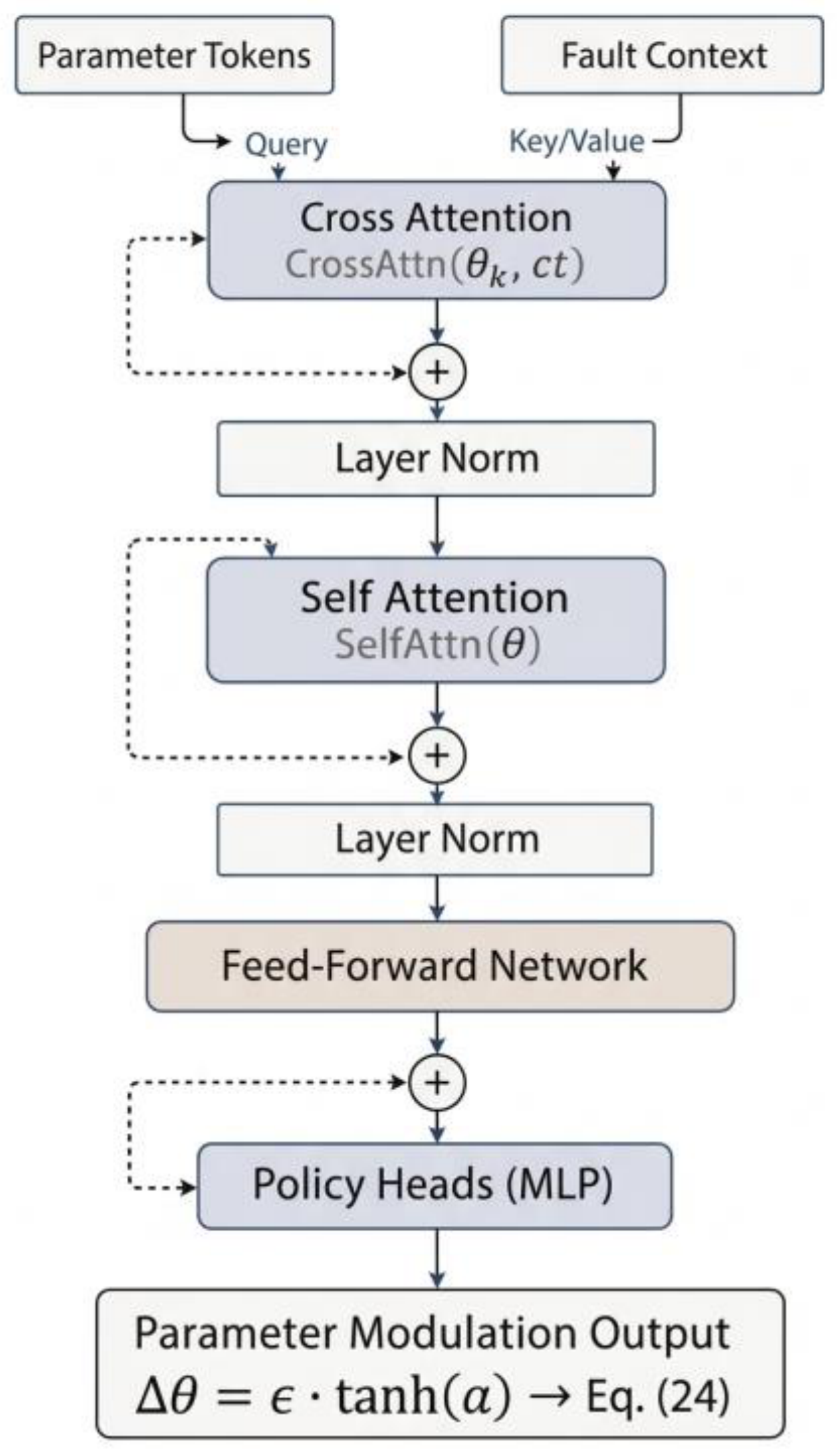
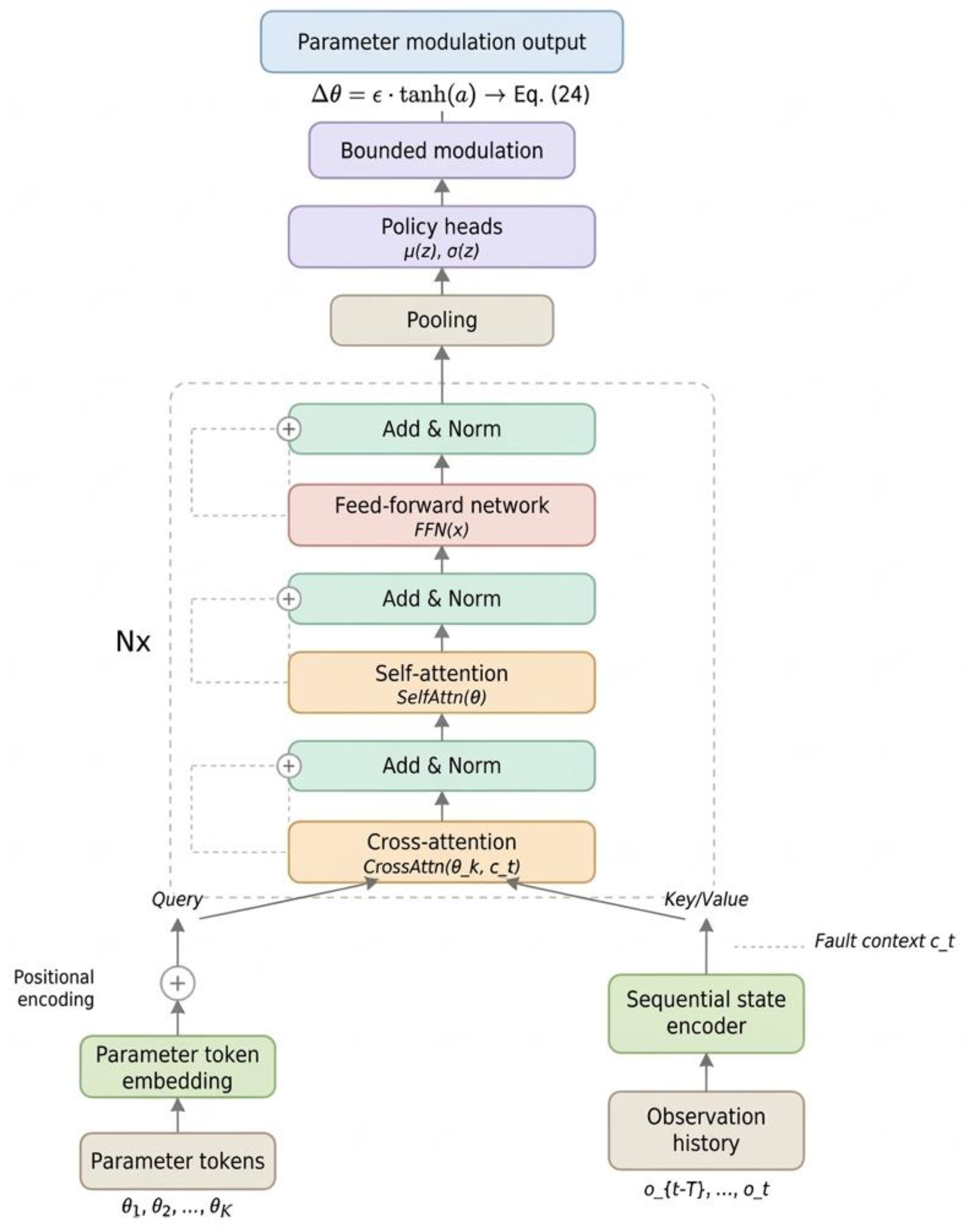
ensuring $\Delta \theta \in [-ϵ,ϵ{]}^N$. This acts as a trust region on parameter space, limiting deviation from nominal design. Figure 3 shows the internal structure of a single Transformer layer repeated L times. Parameter Tokens enter as Query and Fault Context h_c enters as Key/Value into Cross-Attention $\mathrm{CrossAttn}({\theta }_k,ct)$, which integrates fault information into each parameter token. Self-Attention $\mathrm{SelfAttn}\left(\theta \right)$ then allows each parameter token to attend to all others via learned weights ${\alpha }_{ij}$, capturing cross-parameter dependencies. The Feed-Forward Network applies a two-layer MLP $\mathrm{FFN}\left(x\right)=\mathrm{ReLU}(x{W}_1+b_1)W_2+b_2$ with hidden dimension d_ff. Each sublayer is wrapped with residual connection and Layer Norm for training stability. Policy Heads output mean $\mu (\cdot )$ and standard deviation $\sigma (\cdot )$, and the final bounded modulation $\Delta \theta =ϵ\cdot \mathrm{t}\mathrm{a}\mathrm{n}\mathrm{h}\left(a\right)$ constrains the output to $\left[-ϵ,ϵ{]}^N\right.$.

3.4. Training via Proximal Policy Optimization

Based on the belief representation, the adaptive control problem is formulated as an MDP $\left(\mathcal{S},\mathcal{A},\mathcal{P},\mathcal{R},\gamma \right)$. The action space corresponds to bounded parameter modulation:

$$a_t=\Delta {\theta }_t\in {\left[-ϵ,ϵ\right]}^N$$

(25)

The transition dynamics are implicitly defined by the closed-loop system in (6). Rather than optimizing only instantaneous tracking accuracy, the learning objective explicitly emphasizes performance recovery after degradation onset. Let t_f denote the time at which degradation occurs; the recovery cost is defined as:

$$J_{rec}={\int }_{t_f}^{t_f+T_r}{‖e\left(t\right)‖}^{2}dt$$

(26)

where $e\left(t\right)=x\left(t\right)-x_{\mathrm{r}\mathrm{e}\mathrm{f}}\left(t\right)$ and T_r is the recovery horizon.

As illustrated in Figure 4, the Transformer policy network processes two input streams: parameter tokens embedded with positional encoding on the left, and observation history encoded into a fault context representation through a sequential state encoder on the right. These inputs enter the N× repeated Transformer block, where cross-attention integrates fault context as Key/Value with parameter tokens as Query, followed by self-attention to capture cross-parameter dependencies. Each sub-layer is wrapped with residual connections and layer normalization to stabilize gradient flow. The processed token sequence is then pooled and passed through policy heads to produce the mean and variance of a Gaussian distribution, from which actions are sampled. Finally, a bounded modulation function $\Delta \theta =ϵ\cdot \mathrm{t}\mathrm{a}\mathrm{n}\mathrm{h}\left(a\right)$ constrains the output to ensure parameter adjustments remain within a safe trust region around the nominal controller design.

Figure 4 shows how the parameter token stream and observation history stream are combined. On the left, Parameter Tokens ${\theta }_1,\dots ,{\theta }_K$ combined with Positional Encoding form the Query stream, carrying both parameter identity and structural information. On the right, Observation History $o_{t-T},\dots ,o_t$ is processed by the Sequential State Encoder to produce Fault Context $c_t\in {\mathbb{R}}^d$, which encodes temporal fault evolution and enters as Key/Value. Inside the $N\times$ repeated Transformer block, Cross-Attention fuses fault context into each parameter token, Self-Attention captures cross-parameter coupling via learned weights ${\alpha }_{ij}$, and the Feed-Forward Network applies per-token nonlinear transformation, each wrapped with Add\ & Norm. The merged representation is aggregated via Pooling and decoded through Policy Heads to produce mean $\mu \left(z\right)$ and variance $\sigma \left(z\right)$, from which actions are sampled. The Bounded Modulation $\Delta \theta =ϵ\cdot \mathrm{t}\mathrm{a}\mathrm{n}\mathrm{h}\left(a\right)$ enforces the trust region $\left[-ϵ,ϵ{]}^N\right.$ before the modulated parameters are applied.

The instantaneous reward is designed to minimize this objective:

$$r_t=-a_1{‖e(t)‖}^2-a_2{‖u(t)‖}^2-a_3{‖\Delta {\theta }_t‖}^2+a_4{1}_{recovered}$$

(27)

where the recovery indicator is defined as:

$$1_{recovered}=1 \mathrm{if} ‖e(t)‖<{ϵ}_r for t\in \left[t_S,t_S+T_S\right]$$

(28)

Otherwise $1_{recovered}=0$. This explicitly defines recovery success as maintaining tracking error below threshold ${ϵ}_r$ for a sustained duration T_s.

The policy is trained using PPO with the clipped surrogate objective:

$$L^{CLIP}\left(\varphi \right)=E_t\left[{\mathrm{m}\mathrm{i}\mathrm{n}(r_t\left(\varphi \right)\widehat{A}}_t,clip{r}_t\left(\varphi \right),1-\delta ,1+\delta ){\widehat{A}}_t\right]$$

(29)

where $r_t(\varphi )={\displaystyle \frac{{\pi }_{\varphi }(a_t\mid s_t)}{{\pi }_{{\varphi }_{old}}(a_t\mid s_t)}}$ is the probability ratio and ${\widehat{A}}_t$ is the generalized advantage estimate. The advantage is estimated using a critic network $V_{\psi }(s_t)$, which takes the same belief state s_t as input and predicts the expected cumulative discounted return under the current policy. Given the collected rewards $\left\{r_t\right\}$, the generalized advantage estimate (GAE) is computed as:

$${\widehat{A}}_t=\sum _{t=0}^{T-t}{\left(\gamma \lambda \right)}^l{\delta }_{t+i}$$

(30)

where $d_t=r_t+\gamma V_{\psi }(s_{t+1})-V_{\psi }(s_t)$ is the temporal-difference residual, $\gamma$ is the discount factor, $\lambda \in \left[\mathrm{0,1}\right]$ is the GAE smoothing parameter that controls the bias-variance tradeoff, and T is the episode horizon. The critic network is trained by minimizing the mean squared error between its predictions and the observed returns:

$$L^v\left(\psi \right)=E_1\left[{\left(v_{\psi }\left(S_t\right)-{\widehat{R}}_t\right)}^2\right]$$

(31)

where ${\widehat{R}}_t={\sum }_{l=0}^{T-t}{\gamma }^l{r}_{t+l}$ is the discounted return. During each PPO update epoch, the policy parameters $\varphi$ are updated by maximizing $L^{CLIP}\left(\varphi \right)$ while the critic parameters $\psi$ are updated by minimizing $L^V\left(\psi \right)$, forming a joint actor-critic training loop. The critic provides a state-dependent baseline that reduces the variance of policy gradient estimates, enabling stable training under the randomized fault injection described in Algorithm 1. The clipping mechanism provides implicit regularization on policy updates by limiting the deviation between the updated and behavior policies, complementing the bounded modulation constraint. The complete training procedure is summarized in Algorithm 1.

Algorithm 1. Transformer-DRL Parameter Modulation training

Input: Environment E, nominal params θ0, bound ε, hyperparams a1, a2, a3, a4

1:    Initialize policy πϕ (Transformer), value network Vψ

2:    Initialize replay buffer B ← ∅

3:    for episode = 1, 2, …, Nep do

4:        Sample fault scenario ϕa ∼ p(ϕ)

5:        Reset environment; observe s0

6:        for t = 0, 1, …, T do

7:            Encode history: hc = SequentialEncoder(O{t – M + 1:t})                      ▷ Equations (11)–(15)

8:            Tokenize params: Z = ParamEmbedding(θ0)                        ▷ Equations (16) and (17)

9:            Compute (μϕ, σϕ) = TransformerPolicy(Z, hC)                        ▷ Equations (18)–(22)

10:          Sample at ∼ N(${\mathsf{\mu }}_{\mathsf{\varphi }}, {\sigma }_{\psi }^2$)                                    ▷ Equation (23)

11:       Modulate: Δθt = ϵ · tanh(at)                                 ▷ Equation (24)

12:       Apply: θ′_t = θ0$\odot (1_N$+ Δθ_t)                                     ▷ Equation (4)

13:       Execute ut = C(xt, xref, θ′t); observe rt, st+1       ▷ Equation (5)

$14: {\mathrm{r}}_{\mathrm{t}}=-{\mathrm{a}}_1{‖\mathrm{e}\left(\mathrm{t}\right)‖}^2-{\mathrm{a}}_2{‖\mathrm{u}\left(\mathrm{t}\right)‖}^2-{\mathrm{a}}_3{‖\Delta {\mathsf{\theta }}_{\mathrm{t}}‖}^2+{\mathrm{a}}_4{1}_{\mathrm{r}\mathrm{e}\mathrm{c}\mathrm{o}\mathrm{v}\mathrm{e}\mathrm{r}\mathrm{e}\mathrm{d}}$       ▷ Equation (27)

15:       Store (st, at, rt, st+1) in B

16:      end for

17:      Compute advantages Ât via GAE

18:      for k = 1, …, K do

19:       Compute ratio rt(ϕ) = πϕ(at|st)/πϕold(at|st)

20:       LCLIP(ϕ) = Et[min(rt(ϕ)Ât, clip(rt(ϕ), 1 − δ, 1 + δ)Ât)]    ▷ Equation (29)

21:       Update ϕ by maximizing LCLIP(ϕ)

22:       Update ψ by minimizing value loss

23:      end for

24:   end for

25:   return πϕ*

The algorithm proceeds as follows. Lines 1–2 initialize the Transformer policy ${\pi }_{\varphi }$, critic network $V_{\psi }$, and replay buffer. Lines 3–4 sample a randomized fault scenario ${\varphi }_a\sim p(\varphi )$ at the start of each episode, covering diverse fault types and severities to prevent overfitting to specific fault patterns. Line 5 resets the environment. Lines 6–16 execute the inner timestep loop: Line 7 encodes observation history into belief representation h_c via the Sequential State Encoder; Line 8 maps nominal parameters ${\theta }_0$ to token embeddings Z; Line 9 computes the modulation distribution $\left({\mu }_{\varphi },{\sigma }_{\varphi }\right)$ via the Transformer Policy Network; Line 10 samples action $a_t\sim \mathcal{N}({\mu }_{\varphi },{\sigma }_{\varphi }^2)$ for exploration; Lines 11–12 apply the bounded modulation $\Delta {\theta }_t=ϵ\cdot \mathrm{t}\mathrm{a}\mathrm{n}\mathrm{h}\left(a_t\right)$ and compute modulated parameters ${\theta }_t^{\prime }={\theta }_0\odot (1+\Delta {\theta }_t)$; Line 13 executes the modulated controller and observes r_t, $s_{t+1}$; Line 14 computes the reward from Equation (27); Line 15 stores the transition. Line 17 computes generalized advantage estimates ${\widehat{A}}_t$ via GAE to reduce gradient variance. Lines 18–23 perform K epochs of PPO updates by maximizing $L^{CLIP}\left(\varphi \right)$ and minimizing the value loss. Line 25 returns the converged policy ${\pi }_{\varphi }^{*}$.

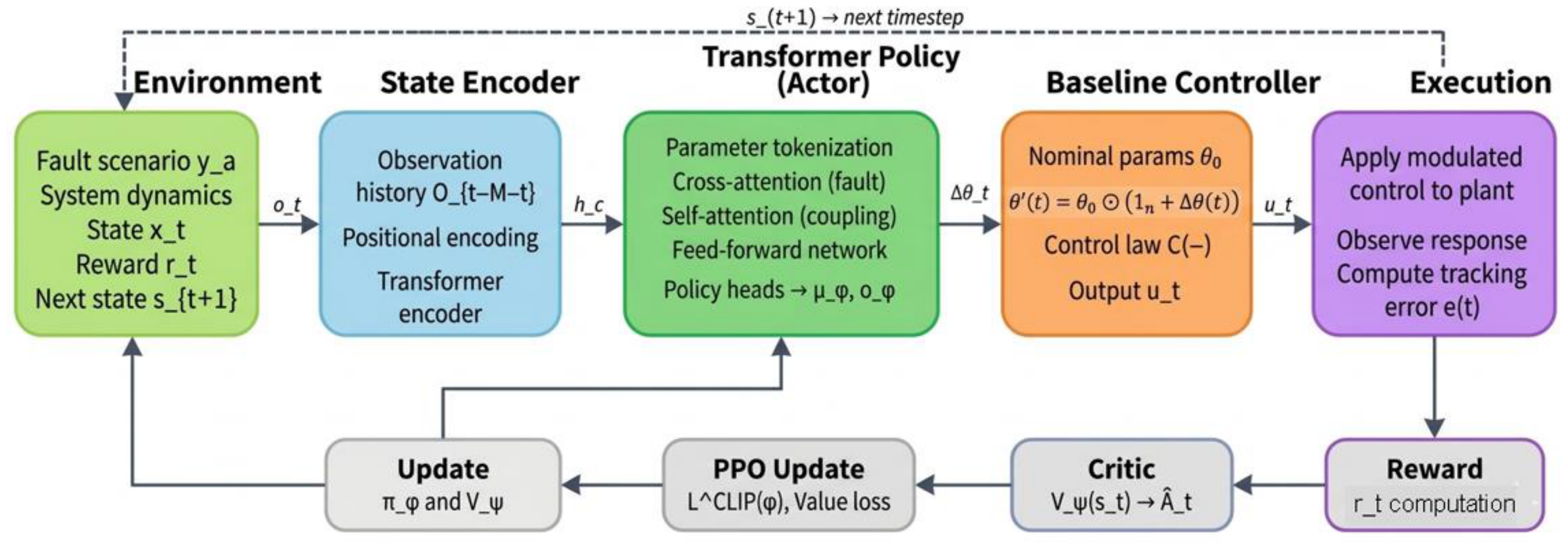
The PPO training loop, as illustrated in Figure 5, operates as a closed-loop interaction between the Transformer policy and the fault-affected environment. At each timestep, the sequential state encoder processes observation history into a belief representation, which the Transformer policy network uses to generate bounded parameter modulation values Δθ_t. These modulated parameters are applied to the baseline controller, which executes control actions on the plant and produces tracking error and reward signals. The Critic network estimates the advantage function from the collected rewards, which drives the PPO clipped surrogate objective to update both the policy and value networks. This process repeats over successive episodes with randomized fault injections, enabling the policy to generalize across diverse fault conditions without fault-specific re-optimization.

Figure 5 shows the closed-loop PPO training process across five functional modules. The Environment block provides fault scenario ${\phi }_a$, system state x_t, reward r_t, and next state $s_{t+1}$. The State Encoder processes observation history $O_{\left\{t-M:t\right\}}$ with positional encoding and a Transformer encoder to produce belief representation h_c. The Transformer Policy (Actor) applies parameter tokenization, cross-attention with fault context, self-attention for cross-parameter coupling, and policy heads to output $\Delta {\theta }_t$ with parameters ${\mu }_{\varphi },{\sigma }_{\varphi }$. The Baseline Controller applies ${\theta }^{\prime }={\theta }_0\odot (1_N+\Delta {\theta }_t)$ via the control law $C(\cdot )$ and outputs u_t. The Execution block applies u_t to the plant and computes tracking error e(t). The Reward block computes r_t from Equation (27). The Critic estimates advantage ${\widehat{A}}_t=V_{\psi }(s_t)$, which drives the PPO Update to maximize $L^{CLIP}(\varphi )$ and update both ${\pi }_{\varphi }$ and $V_{\psi }$.

3.5. Stability Analysis

The proposed framework applies bounded parameter modulations $\Delta \theta \left(t\right)\in [-ϵ,ϵ{]}^N$ to the baseline controller, which can be interpreted as a structured perturbation to the nominal closed-loop system. The following result establishes the uniform ultimate boundedness of the modulated closed-loop system.

Assumption 1. 

The nominal closed-loop system under $C(\cdot ,{\theta }_0)$ is asymptotically stable, admitting a continuously differentiable Lyapunov function $V\left(x\right)$ satisfying $\dot{V}(x)\le -{\alpha }_3(\parallel x\parallel )$ along nominal trajectories, for some class ${\mathcal{K}}_{\infty }$ functions ${\alpha }_3$ and ${\alpha }_4$, where $\parallel {\displaystyle \mathit{\nabla }}V\left(x\right)\parallel \le {\alpha }_4(\parallel x\parallel )$.

Assumption 2. 

The closed-loop vector field is locally Lipschitz in $\theta$ with constant $L>0$:

$$\begin{gathered} ‖f\left(x,C\left(x,x_{ref,}{\theta }_1\right),{\varphi }_a\right),-f\left(\left(x,C\left(x,x_{ref,}{\theta }_2\right),{\varphi }_a\right)\right)‖ \\ \le L‖{\theta }_1-{\theta }_2‖ \end{gathered}$$

(32)

for all $x\in \mathcal{X}$ and all ${\theta }_1,{\theta }_2$ in a neighborhood of ${\theta }_0$. Since ${\theta }^{\prime }(t)={\theta }_0\odot (1_N+\Delta \theta (t))$, it follows that $\parallel {\theta }^{\prime }-{\theta }_0\parallel \le c\parallel \Delta \theta \parallel$, where $c=\parallel {\theta }_0{\parallel }_{\infty }$ is a constant determined by the nominal parameter vector.

Proposition 1. 

Under Assumptions 1 and 2, the state of the modulated closed-loop system (6) is uniformly ultimately bounded (UUB):

$$‖x\left(t\right)‖\le \beta (‖x\left(0\right)‖,t)+\sigma \left(ϵ\right)$$

(33)

for some class $\mathcal{K}\mathcal{L}$ function $\beta$ and class $\mathcal{K}$ function $\sigma$.

Proof. 

Let $k=cL\sqrt{N}$, where c and L are defined in Assumption 2. Denote the nominal and modulated vector fields respectively as $f_{nom}(x)=f(x,C(x,x_{ref},{\theta }_0),{\varphi }_a)$ and $f_{mod}(x)=f(x,C(x,x_{ref},{\theta }^{\prime }(t)),{\varphi }_a)$. Evaluating $\dot{V}(x)$ along trajectories of the modulated system (6) and adding and subtracting the nominal dynamics:

$$\begin{gathered} \dot{v}\left(x\right)=\nabla \vee {\left(x\right)}^T{f}_{nom}\left(x\right)+\nabla \vee {\left(x\right)}^T\left(f_{mod}\left(x\right)-f_{nom}\left(x\right)\right) \\ \le -a_3\left(‖x‖\right)+a_4\left(‖x‖\right)·\mathrm{k}ϵ \end{gathered}$$

(34)

where we have used Assumptions 1 and 2, and the fact that the tanh constraint (24) enforces $\parallel \Delta \theta \parallel \le ϵ\sqrt{N}$ strictly. Therefore $\dot{V}(x)<0$ holds for all x outside the compact set:

$$\mathsf{\Omega }=\left\{x:a_3\left(‖x‖\right)\ge a_4\left(‖x‖\right)·\mathrm{k}ϵ\right\}$$

(35)

By standard Lyapunov arguments, all trajectories originating outside $\mathsf{\Omega }$ converge to $\mathsf{\Omega }$ in finite time and remain therein, establishing UUB of the closed-loop state. □

Remark 3. 

The ultimate bound $\mathit{\Omega }$ shrinks as $ϵ\to 0$, and the system behavior approaches that of the nominal asymptotically stable system. In practice, $ϵ$ is selected via grid search to balance recovery performance against the residual tracking error within $\mathit{\Omega }$.

The theoretical analysis in Section 3.5 establishes that the modulated closed-loop system remains uniformly ultimately bounded under the bounded parameter modulation constraint (24), with the ultimate bound Ω determined by the modulation bound ε and the system Lipschitz constant. While this provides formal guarantees on closed-loop stability, it does not directly characterize the practical recovery performance achievable by the learned policy under diverse fault conditions. To empirically evaluate the effectiveness of the proposed framework, the following section presents comparative experiments across three control systems, examining whether the Transformer-based policy can exploit the allowable modulation range [−ε, ε]^N to achieve fast and accurate fault recovery while remaining consistent with the stability conditions established in Proposition 1.

4. Experimental Results

4.1. Comparison Study with Genetic Algorithm-Based Neural Network

To evaluate the effectiveness of the proposed Transformer-based DRL method for fault-tolerant control, comparative simulations are conducted using the quadrotor dynamics model and experimental setup reported by [27]. The same physical parameters, reference trajectory (from the origin to $\left[-2,2,2\right]$ m), and actuator loss-of-effectiveness fault model (${\lambda }_3=0.7$) are adopted to ensure a fair comparison. Four control strategies are considered: manual PID tuning via trial-and-error, GA-based tuning under fault-free conditions (GA–normal), GA-based tuning with prior knowledge of the fault scenario (GA–fault), and the proposed DRL + Transformer approach, which employs a single unified policy for adaptive parameter modulation. Performance is evaluated using the Integral Squared Error (ISE) over a 5-s flight duration. The quantitative comparison results are summarized in

Table 1. Fault-Tolerant Control Performance Comparison (ISE).

Method	No Fault	${\mathit{\lambda }}_3$ = 0.7 Fault
Manual	2.8357	22.1196
GA (normal tuning)	0.8047	1.1897
GA (fault tuning)	1.0533	0.9820
DRL + Transformer	0.7853	0.9644

.

The results show that the proposed DRL + Transformer controller achieves consistently low ISE values in both nominal and faulty conditions, with ISEs of 0.7853 (no fault) and 0.9644 (${\lambda }_3=0.7$). Compared with GA-based controllers, which require either fault-free assumptions or prior fault knowledge for tuning, the proposed method attains comparable or better performance using a single policy without fault-specific re-optimization. This demonstrates its ability to maintain control performance across varying fault conditions while improving adaptability and practical applicability.

4.2. Comparison Study with PSO-Based Optimal Gain Scheduling Backstepping Controller

To evaluate the effectiveness of the proposed Transformer-based DRL method for transformable quadrotor control, comparative simulations are conducted using the quadrotor dynamics model and experimental setup reported by [28]. The same physical parameters, inertia configurations for six morphological states, and configuration switching schedules are adopted to ensure a fair comparison. Two representative scenarios are designed: (1) circular trajectory tracking, where the quadrotor follows a circular path with radius 2 m while ascending at 13/150 m/s over 150 s, with configuration switches at t = 0, 25, 50, 75, 100, and 125 s; (2) waypoint trajectory tracking, where the quadrotor navigates through a sequence of waypoints from origin to (0, 0, 10), (4, 0, 10), (4, 4, 10), (0, 4, 10), and back to (0, 0, 10) over 90 s, with configuration switches at t = 0, 5, 20, 40, 60, and 80 s. Two control strategies are compared: the PSO-based optimal gain scheduling backstepping controller (PSO-Backstepping) proposed in the original work, and the proposed DRL + Transformer approach. Performance is evaluated using the maximum absolute tracking errors for position (x, y, z) and attitude (φ, θ, ψ).

4.2.1. Scenario 1: Circular Trajectory Tracking Results

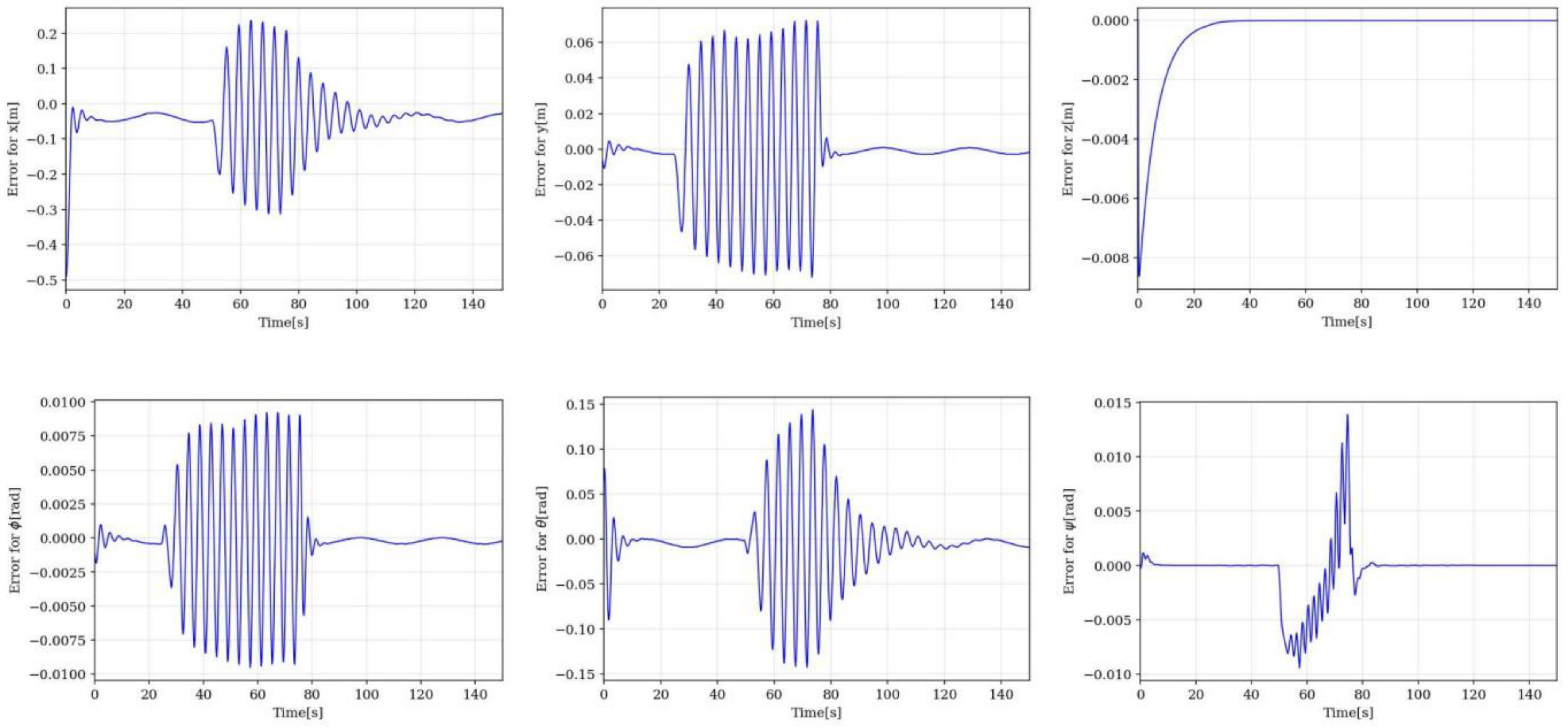
The tracking performance for the circular trajectory is illustrated in Figure 6. The position errors remain bounded within ±0.25 m along the x-axis, ±0.07 m for y-axis, and ±0.008 m for z-axis. The altitude error exhibits rapid convergence from an initial transient to near-zero steady-state within 20 s. The attitude errors are maintained within ±0.01 rad for roll, ±0.15 rad for pitch, and ±0.015 rad for yaw. Increased oscillations are observed during the 50–80 s interval corresponding to configuration transitions, yet the controller successfully attenuates these disturbances and restores tracking accuracy. Compared with the PSO-Backstepping method reported in [28], the proposed approach demonstrates tighter error bounds across all axes, with particularly notable improvement in altitude tracking where sub-centimeter precision is achieved.

4.2.2. Scenario 2: Waypoint Trajectory Tracking Results

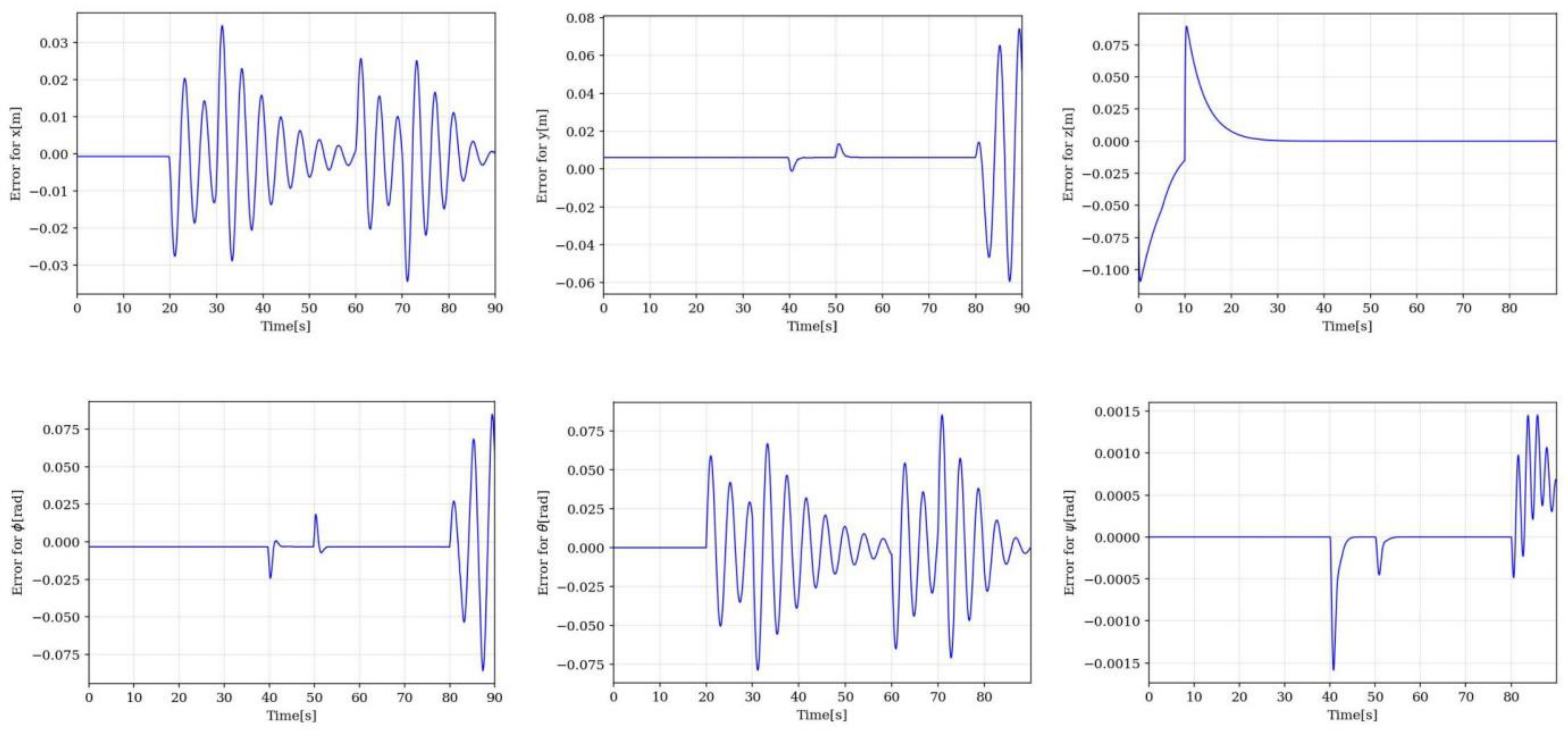
The results for the waypoint trajectory are shown in Figure 7. The position errors are bounded within ±0.035 m for x-axis, ±0.075 m for y-axis, with the altitude error showing a brief initial overshoot of 0.1 m before converging to zero within 20 s. The attitude errors remain within ±0.085 rad for roll, ±0.08 rad for pitch, and remarkably ±0.0015 rad for yaw. Transient spikes in roll and pitch errors are observed at waypoint transitions (t ≈ 40 s, 80 s), but rapid recovery is achieved within 2–3 s. The proposed method exhibits superior tracking precision compared to the PSO-Backstepping baseline, particularly in altitude and yaw regulation where near-zero steady-state errors are maintained throughout the mission.

4.3. Comparison Study with TD3 Reinforcement Learning for PI Controller Gain Scheduling

To evaluate the effectiveness of the proposed Transformer + PPO method for fault-tolerant control, comparative simulations are conducted based on the PMDC motor model and experimental setup reported by [29]. The same motor parameters and reference trajectory are adopted to ensure a fair comparison. Following the original paper, two identical fault scenarios are considered: (1) a bias fault with amplitude of 2 injected at t = 5 s, representing sensor calibration drift, and (2) a sinusoidal fault f(t) = 2sin (t) injected at t = 5 s, representing time-varying disturbances. Since the original paper does not provide specific quantitative data for fault-tolerant control performance, we reproduced the experiments and evaluated the post-fault period (5–10 s) using RMSE, IAE, overshoot, recovery time, and steady-state error. The quantitative comparison results are summarized in

Table 2. Performance Comparison under Bias Fault Scenario.

Performance Metric	TD3	Transformer + PPO
Overshoot at fault	0.12	0.08
Recovery time (s)	0.45	0.32
Steady-state error	0.023	0.015
RMSE (5–10 s)	0.089	0.064
IAE (5–10 s)	0.156	0.137

and

Table 3. Performance Comparison under Sinusoidal Fault Scenario.

Performance Metric	TD3	Transformer + PPO
Overshoot at fault	0.38	0.19
Recovery time (s)	0.62	0.33
Steady-state error	0.044	0.019
RMSE (5–10 s)	0.165	0.073
IAE (5–10 s)	0.412	0.188

.

4.3.1. Scenario 1: Bias Fault Experiment

As shown in Table 2, the proposed Transformer + PPO method outperforms the baseline TD3 + PI approach across all metrics under the bias fault scenario. The overshoot at fault injection is reduced from 0.12 to 0.08, indicating a faster and smoother transient response when the fault occurs. The recovery time decreases from 0.45 s to 0.32 s, demonstrating that the proposed method can restore tracking performance more quickly. In terms of tracking accuracy, the steady-state error is reduced from 0.023 to 0.015, and the RMSE decreases from 0.089 to 0.064. The IAE is also improved from 0.156 to 0.137. These improvements are attributed to the following mechanism. A constant bias fault of amplitude 2 injected at $t=5\mathrm{s}$ introduces a persistent additive offset into the sensor readings, causing the nominal PI controller to develop a systematic steady-state error. The sequential state encoder accumulates the observation history over the preceding M timesteps, allowing it to identify the sustained unidirectional deviation in the error signal as a signature of constant bias rather than transient disturbance. This temporal pattern is encoded into the belief representation h_c, which is then passed to the cross-attention mechanism as Key and Value. The cross-attention layer uses h_c to condition each parameter token, enabling the policy to infer that the integral gain requires upward adjustment to eliminate the bias-induced offset. Because this adaptation occurs within the Transformer policy rather than through re-optimization, the response is immediate: the modulated parameters ${\theta }^{\prime }\left(t\right)$ are updated at every timestep, reducing both the initial overshoot and the time required to reach the recovery threshold ${ϵ}_r$. The TD3 + PI baseline, relying on a fixed MLP policy without explicit temporal context, cannot distinguish persistent bias from transient noise as efficiently, resulting in slower convergence and higher residual error. These results demonstrate that the proposed Transformer + PPO method can effectively compensate for constant sensor bias with faster response and better tracking accuracy.

4.3.2. Scenario 2: Sinusoidal Fault Experiment

As shown in Table 3, the proposed Transformer + PPO method demonstrates more significant improvements under the sinusoidal fault scenario compared to the bias fault case. The overshoot at fault injection is reduced from 0.38 to 0.19, representing a 50% improvement. The recovery time decreases substantially from 0.62 s to 0.33 s, indicating much faster fault compensation capability. For tracking accuracy, the steady-state error is reduced from 0.044 to 0.019, and the RMSE decreases from 0.165 to 0.073, achieving over 55% improvement. The IAE is also significantly improved from 0.412 to 0.188. These superior results are attributed to the Transformer’s capability in modeling temporal dependencies, which enables better adaptation to time-varying fault characteristics. The results confirm that the proposed approach is particularly effective for dynamic fault compensation scenarios.

4.4. Case Study

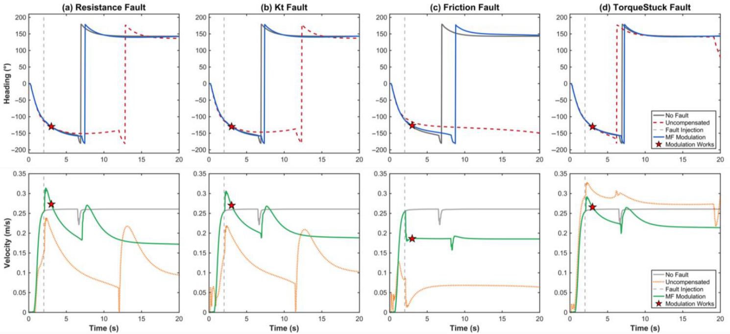
The proposed method is validated on a differential-drive mobile robot, which follows standard DC motor equations [30,31]. Figure 8 shows the heading and velocity recovery comparison under four fault types with different severity levels.

To evaluate the generalization capability of the proposed method, experiments are conducted on a differential-drive wheeled mobile robot under four representative motor fault categories, with fault severity selected to represent moderate-to-severe degradation scenarios (50–70%) that challenge the controller while remaining within recoverable bounds. (a) Resistance fault (50%, left wheel): causes significant heading deviation after fault onset; the DRL-learned MF modulation policy substantially reduces heading deviation, achieving 41% improvement over uncompensated response while maintaining higher velocity. (b) Torque constant (Kt) reduction fault (60%, left wheel): results in velocity drop and heading oscillation; the learned policy improves velocity recovery while smoothing heading transitions through coordinated MF adjustments. (c) Friction fault (50%, right wheel): induces heading drift due to asymmetric wheel response; the policy reduces deviation amplitude and sustains a more consistent velocity profile. This is achieved because the sequential state encoder detects the asymmetric torque imbalance between wheels from the observation history, and the self-attention mechanism coordinates the left and right motor parameter tokens to restore torque balance, counteracting the drift and stabilizing the velocity profile. (d) Torque-stuck fault (70%, left wheel): produces severe heading divergence and velocity collapse; MF modulation mitigates the divergence trend, though performance remains constrained by fundamental actuation loss. Across all fault types, the PPO-trained Transformer policy (green) demonstrates improved tracking compared to uncompensated response (red), with heading and velocity profiles closer to the fault-free baseline (blue). The dashed line indicates fault onset. The policy generalizes across all four fault types despite training only on randomized fault configurations. This is because randomized fault injection during training forces the policy to learn fault-type-agnostic response patterns based on observable consequences such as tracking error and velocity imbalance, rather than fault identity. The self-attention mechanism further supports generalization by dynamically computing attention weights ${\alpha }_{ij}$ from current token representations, enabling context-dependent cross-parameter coordination that adapts to different fault signatures without requiring separate policies. This validates the architecture’s capacity for unified fault-tolerant control across heterogeneous fault conditions.

5. Discussion

The experimental results indicate consistent performance improvements compared with existing fault-tolerant control approaches, highlighting important differences in adaptability characteristics among different methodologies. Previous studies have noted that metaheuristic optimization techniques, such as GA and PSO, typically require offline optimization tailored to specific operating conditions [23]. The results presented in Table 1 are consistent with this observation. GA-based tuning achieves strong performance when optimization is conducted with prior knowledge of the fault scenario (ISE = 0.9820), whereas GA tuned under nominal operating conditions exhibits performance degradation when faults occur. In contrast, the proposed method maintains relatively low ISE values across both nominal and faulty conditions using a unified policy, suggesting improved generalization capability without requiring fault-specific re-optimization. Similarly, the PSO-based gain scheduling backstepping controller proposed by [28] relies on pre-computed gain schedules associated with different system configurations. The proposed approach instead performs online parameter adaptation and demonstrates reduced tracking errors across configuration switching scenarios. These observations suggest that reinforcement learning-based parameter modulation may provide improved adaptability by directly optimizing recovery performance through environment interaction, rather than relying solely on offline optimization procedures.

The improved performance observed under time-varying fault conditions appears to be associated with the Transformer-based policy architecture. Compared with the TD3 + PI method reported by [29], which employs a conventional MLP policy network, the proposed method achieves substantial reductions in RMSE and recovery time under sinusoidal fault disturbances. This improvement may be related to the ability of attention-based architectures to capture long-range temporal correlations, as previously demonstrated in fault diagnosis and time-series modeling tasks [4]. In the proposed framework, the sequential state encoder extracts latent belief representations from observation history, which helps mitigate partial observability caused by delayed or noisy fault estimates. Furthermore, the parameter tokenization mechanism allows the self-attention layers to model potential coupling relationships among controller parameters. Such coordinated parameter modulation may be beneficial for controllers with inherently interdependent parameters, such as ANFIS membership functions. These architectural features differentiate the proposed approach from conventional DRL-based parameter tuning methods that treat controller parameters independently. Nevertheless, further ablation studies would be valuable to isolate the individual contributions of temporal modeling, cross-attention, and parameter tokenization.

Despite the demonstrated performance improvements, several limitations remain. First, the recovery capability is fundamentally constrained by the structural characteristics of the baseline controller. As observed in the torque-stuck fault scenario, parameter modulation alone cannot fully compensate for severe actuation loss, which is consistent with findings reported by [25]. Second, the proposed method assumes that fault type and severity information are available from upstream fault detection and isolation (FDI) modules. In practical implementations, estimation noise and diagnostic latency may degrade recovery performance, particularly under rapidly evolving fault conditions. Third, the current framework provides stability guarantees in the form of uniform ultimate boundedness under bounded parameter modulation; however, formal Lyapunov-based certification for safety-critical deployment remains an open challenge.

6. Conclusions

This paper proposed a Transformer-based deep reinforcement learning framework for adaptive controller parameter modulation in fault recovery. The method introduces parameter tokenization to model cross-parameter dependencies, a sequential state encoder to capture temporal fault evolution, and a fault-aware cross-attention mechanism to enable context-guided parameter adjustment. Experimental results across multiple control systems demonstrate that the proposed approach consistently improves tracking accuracy and recovery performance under diverse fault conditions, while exhibiting strong generalization capability. Future work will focus on incorporating Lyapunov-constrained reinforcement learning to provide formal stability guarantees, extending the framework to handle multiple and cascading faults, integrating control allocation to address fundamental actuation limitations under severe fault scenarios, developing sim-to-real transfer strategies for real-world deployment, and exploring hierarchical architectures that combine parameter modulation with task planning for long-horizon autonomous fault recovery.

References

1. Yazdjerdi, P.; Meskin, N. Actuator fault detection and isolation of differential drive mobile robots using multiple model algorithm. In Proceedings of the 2017 4th International Conference on Control, Decision and Information Technologies (CoDIT), Barcelona, Spain, 5–7 April 2017; IEEE: New York, NY, USA, 2017; pp. 439–443. [Google Scholar]
2. Yazdjerdi, P.; Meskin, N. Design and real-time implementation of actuator fault-tolerant control for differential-drive mobile robots based on multiple-model approach. Proc. Inst. Mech. Eng. Part I J. Syst. Control Eng. 2018, 232, 652–661. [Google Scholar] [CrossRef] [Scilit]
3. Sun, H.; Zhao, S. Fault diagnosis for bearing based on 1DCNN and LSTM. Shock Vib. 2021, 2021, 1221462. [Google Scholar] [CrossRef] [Scilit]
4. Liu, J.; Wang, G.; Hu, P.; Duan, L.Y.; Kot, A.C. Global context-aware attention LSTM networks for 3D action recognition. In Proceedings of the IEEE Conference on Computer Vision and Pattern Recognition, Honolulu, HI, USA, 21–26 July 2017; pp. 1647–1656. [Google Scholar]
5. Lundgren, A.; Jung, D. Data-driven fault diagnosis analysis and open-set classification of time-series data. Control Eng. Pract. 2022, 121, 105006. [Google Scholar] [CrossRef] [Scilit]
6. Ma, Z.L.; Li, X.J. A data-driven fault isolation and estimation approach for unknown linear systems. J. Process Control 2023, 124, 118–128. [Google Scholar] [CrossRef] [Scilit]
7. Parzinger, M.; Hanfstaengl, L.; Sigg, F.; Spindler, U.; Wellisch, U.; Wirnsberger, M. Residual analysis of predictive modelling data for automated fault detection in building’s heating, ventilation and air conditioning systems. Sustainability 2020, 12, 6758. [Google Scholar] [CrossRef] [Scilit]
8. Zhu, F.; Shan, Y.; Tang, Y. Actuator and sensor fault detection and isolation for uncertain switched nonlinear system based on sliding mode observers. Int. J. Control Autom. Syst. 2021, 19, 3075–3086. [Google Scholar] [CrossRef] [Scilit]
9. Tran, A.M.D.; Vu, T.V. Robust MIMO LQR control with integral action for differential drive robots: A Lyapunov-cost function approach. Eng. Technol. Appl. Sci. Res. 2025, 15, 24775–24781. [Google Scholar] [CrossRef] [Scilit]
10. Karaboga, D.; Kaya, E. Adaptive network based fuzzy inference system (ANFIS) training approaches: A comprehensive survey. Artif. Intell. Rev. 2019, 52, 2263–2293. [Google Scholar] [CrossRef] [Scilit]
11. Shi, P.; Wang, X.; Meng, X.; He, M.; Mao, Y.; Wang, Z. Adaptive fault-tolerant control for open-circuit faults in dual three-phase PMSM drives. IEEE Trans. Power Electron. 2022, 38, 3676–3688. [Google Scholar] [CrossRef] [Scilit]
12. Stavrinidis, S.; Zacharia, P. An ANFIS-based strategy for autonomous robot collision-free navigation in dynamic environments. Robotics 2024, 13, 124. [Google Scholar] [CrossRef] [Scilit]
13. Zhong, K.; Yang, Z.; Yu, S.; Li, K. Deep reinforcement learning-based multi-layer cascaded resilient recovery for cyber-physical systems. IEEE Trans. Serv. Comput. 2024. [Google Scholar]
14. Nikanjam, A.; Morovati, M.M.; Khomh, F.; Ben Braiek, H. Faults in deep reinforcement learning programs: A taxonomy and a detection approach. Autom. Softw. Eng. 2022, 29, 8. [Google Scholar] [CrossRef] [Scilit]
15. Wang, X.; Abtahi, S.M.; Chahari, M.; Zhao, T. An adaptive neuro-fuzzy model for attitude estimation and control of a 3 DOF system. Mathematics 2022, 10, 976. [Google Scholar] [CrossRef] [Scilit]
16. Lawrence, N.P.; Forbes, M.G.; Loewen, P.D.; McClement, D.G.; Backström, J.U.; Gopaluni, R.B. Deep reinforcement learning with shallow controllers: An experimental application to PID tuning. Control Eng. Pract. 2022, 121, 105046. [Google Scholar] [CrossRef] [Scilit]
17. Joseph, S.B.; Dada, E.G.; Abidemi, A.; Oyewola, D.O.; Khammas, B.M. Metaheuristic algorithms for PID controller parameters tuning: Review, approaches and open problems. Heliyon 2022, 8, e09399. [Google Scholar] [CrossRef] [Scilit]
18. Süpürtülü, M.; Hatipoğlu, A.; Yılmaz, E. An analytical benchmark of feature selection techniques for industrial fault classification leveraging time-domain features. Appl. Sci. 2025, 15, 1457. [Google Scholar] [CrossRef] [Scilit]
19. Wang, L.; Zhao, W.; Liu, Z.; Dang, Q.; Zou, X.; Wang, K. Incipient fault detection and reconstruction using an adaptive sliding-mode observer for the actuators of fixed-wing aircraft. Aerospace 2023, 10, 422. [Google Scholar] [CrossRef] [Scilit]
20. Vaswani, A.; Shazeer, N.; Parmar, N.; Uszkoreit, J.; Jones, L.; Gomez, A.N.; Kaiser, Ł.; Polosukhin, I. Attention is all you need. Adv. Neural Inf. Process. Syst. 2017, 30, 5998–6008. [Google Scholar]
21. Surur, K.; Kabir, I.; Ahmad, G.; Abido, M.A. Optimal gain scheduling for fault-tolerant control of quadrotor UAV using genetic algorithm-based neural network. Arab. J. Sci. Eng. 2025, 1–15. [Google Scholar] [CrossRef] [Scilit]
22. Derrouaoui, S.H.; Bouzid, Y.; Guiatni, M. PSO based optimal gain scheduling backstepping flight controller design for a transformable quadrotor. J. Intell. Robot. Syst. 2021, 102, 67. [Google Scholar] [CrossRef] [Scilit]
23. Kuryło, P. Modeling of two-wheeled self-balancing robot driven by DC gearmotors. Int. J. Appl. Mech. Eng. 2017, 22, 739–747. [Google Scholar]
24. Moritz, J.; Musa, M.; Wejinya, U. Design and modeling of a two-wheeled differential drive robot. Int. J. Control Autom. Syst. 2024, 22, 2273–2282. [Google Scholar] [CrossRef] [Scilit]
25. Sardashti, A.; Nazari, J. A learning-based approach to fault detection and fault-tolerant control of permanent magnet DC motors. J. Eng. Appl. Sci. 2023, 70, 109. [Google Scholar] [CrossRef] [Scilit]
26. Ye, S.; Jiang, J.; Li, J.; Liu, Y.; Zhou, Z.; Liu, C. Fault diagnosis and tolerance control of five-level nested NPP converter using wavelet packet and LSTM. IEEE Trans. Power Electron. 2019, 35, 1907–1921. [Google Scholar] [CrossRef] [Scilit]
27. Shen, Q.; Shi, P.; Lim, C.P. Fuzzy adaptive fault-tolerant stability control against novel actuator faults and its application to mechanical systems. IEEE Trans. Fuzzy Syst. 2024, 32, 2331–2340. [Google Scholar] [CrossRef] [Scilit]
28. Kong, N.J.; Li, C.; Council, G.; Johnson, A.M. Hybrid iLQR model predictive control for contact implicit stabilization on legged robots. IEEE Trans. Robot. 2023, 39, 4712–4727. [Google Scholar] [CrossRef] [Scilit]
29. Pan, J.; Qu, L.; Peng, K. Deep residual neural-network-based robot joint fault diagnosis method. Sci. Rep. 2022, 12, 17158. [Google Scholar] [CrossRef] [Scilit] [PubMed]
30. Lakhani, A.I.; Chowdhury, M.A.; Lu, Q. Stability-preserving automatic tuning of PID control with reinforcement learning. arXiv 2021, arXiv:2112.15187. [Google Scholar] [CrossRef] [Scilit]
31. Mehta, N.S.; Bhaiya, V.; Patel, K.A.; Farsangi, E.N. Predictive active control of building structures using LQR and artificial intelligence. Earthq. Eng. Eng. Vib. 2024, 23, 489–502. [Google Scholar] [CrossRef] [Scilit]
Figure 1. DRL-Transformer Method Structure.
Mathematics 14 01409 g001
Figure 2. Architecture of the Proposed Transformer-Based Parameter Modulation Method.
Mathematics 14 01409 g002
Figure 3. Architecture of the Transformer Policy Network.
Mathematics 14 01409 g003
Figure 4. PPO Network Architecture for Adaptive Parameter Modulation.
Mathematics 14 01409 g004
Figure 5. PPO training loop for adaptive parameter modulation.
Mathematics 14 01409 g005
Figure 6. Position and Attitude errors under Scenario 1.
Mathematics 14 01409 g006
Figure 7. Position and Attitude errors under Scenario 2.
Mathematics 14 01409 g007
Figure 8. Heading (top, degrees) and velocity (bottom, m/s) recovery comparison under four motor fault types on a differential-drive mobile robot. Blue: fault-free baseline; Red: uncompensated fault response (dashed line = fault onset); Green: proposed DRL + Transformer modulation policy. (a) Resistance fault (50%, left wheel): persistent heading deviation. (b) Kt reduction fault (60%, left wheel): velocity drop and heading oscillation. (c) Friction fault (50%, right wheel): asymmetric heading drift. (d) Torque-stuck fault (70%, left wheel): severe divergence and velocity collapse; modulation partially mitigates but remains limited by actuation loss.
Mathematics 14 01409 g008