Closed-Form Almost Periodical Solutions for a Dynamical System Using the Optimal Auxiliary Functions Method

Abstract

The main aim of our paper is concerning the damped oscillations of 3D dynamical systems, depending on a single physical parameter. This system does not admit Hamilton–Poisson structure but can be explicitly integrated, and the exact parametric solutions are built via a smooth function. The influence of the physical parameter is semi-analytically analyzed using the Optimal Auxiliary Functions Method (OAFM). One of the advantages of the applied method is the small number of iterations due to the appropriate choice of auxiliary convergence control functions. The OAFM solutions are effectively in good agreement with corresponding numerical ones, represented qualitatively by figures and quantitatively by tables. The statistical tests of residuals highlighted the accuracy of our results. The proposed method can be considered an analytical tool for nonlinear vibration analysis of numerous applications from electrical engineering or mechanical structures based on damped rotatory oscillators to the field of image encryption.

1. Introduction

The phenomenon of chaos is an intensively studied topic. Lorenz was the first to define chaotic systems as dynamical systems governed by nonlinear differential equations, characterized by a high sensitivity to initial conditions. Although the system is deterministic, its evolution over time remains practically unpredictable. Subsequently, similar chaotic systems were developed and analyzed, including the Rössler system, the Chen system, the Lü system, and the Liu systems [1]. In 2002, a unified chaotic system was proposed that connects the Chen system and the Lorenz system through the chaotic attractor specific to the Lü system. A characteristic of the Lorenz-type system families is the presence of two quadratic terms in the right-hand side of the equations.

Chaotic systems are of great interest to researchers due to their complex behavior, characterized by sensitivity to initial conditions, unpredictability, and a large continuous spectrum. These features make them useful in numerous engineering applications, such as secure communication, cryptography, voice encryption, image encryption, robotics, fluid dynamics experiments, secure medical imaging, electrical circuits, economics, and biology [2,3,4,5,6,7,8,9,10].

Many researchers have focused their attention on the chaotic behavior of 3D dynamical systems. Suneja et al. [3] investigated a new three-dimensional chaotic system, different from the Lorenz system, with seven terms, two quadratic nonlinearities, and four parameters, used in text data encryption, using a three-key mixing algorithm. Liu [4] proposed a real-time encryption and description scheme to solve the secure communication required for instant audio messaging in the absence of a secure communication channel, designing a new two-channel audio block encryption scheme. It uses a 3D chaotic system for this, generating initial values of the chaotic system based on random external values and the hash value of the simple sound. Ye and Wang [5] performed numerical simulations for a rarely used dynamical (3D) system with an exponential term. The sum of the Lyapunov exponents for the proposed system is 0, so the system can generate not a single attractor but an infinite set of attractors. Wang [6] proposed a new autonomous 3D chaotic system and investigated its dynamic behavior. The proposed system can generate chaotic attractors. An adaptive control of sliding modes is developed. Gao and Wang [7] introduced an image encryption algorithm using the Sprott K system. Zhou et al. [8] analyzed a novel three-dimensional conservative memristive system capable of generating a large-scale multi-scroll rotational attractor. Yang et al. [9] introduced a 3D chaotic system with an innovative “double scroll” structure using additional nonlinear functions, which was used in underwater acoustic signal detection. Khattar et al. [10] introduced a novel chaotic system including an exponential nonlinear term and developed a synchronization scheme between six actuators and four response systems for the first time. Also, the concepts of compound synchronization and compound combined synchronization were extended to compound combined dual synchronization, which involves ten chaotic systems.

The practicality of the chaotic system with hidden attractors was verified by circuit simulations. Adaptive synchronization offset control and amplification of the use of an investigation of the utility of the proposed chaotic system in engineering applications was investigated by Wang et al. in [11]. In [12], Stroita et al. presented a study on the system identification of a hydraulic cylinder controlled by a servo valve operating under variable load, in hydraulic actuators with variable load, such as those used in wind turbine blade pitch systems. Experimental data collected by a proposed data path system is used for dynamic identification of hydraulics using periodic signals as commands. Khairudin developed an efficient dynamic model, along with a detailed analysis of the behavior of a three-dimensional (3D) crane system with implicit load [13]. The dynamic equations of motion were formulated based on the Lagrange method and nonlinear differential equations. The system dynamics study was carried out using MATLAB/Simulink to highlight the behavior of the 3D crane in both the time and frequency domains.

Gholamin et al. [14] investigated a new three-dimensional chaotic system, different from the Lorenz system. Tong [15] proposed a forming mechanism of the dynamical structure introducing a constant control signal. Deng et al. [16] numerically simulated one (3D) dynamical system with an exponential term.

Beyond chaotic behaviors, certain 3D dynamical systems can admit asymptotic behaviors, damped oscillations, or periodic oscillations that are due to the effects of some physical parameters. Such properties can be modeled using the two prime integrals Hamiltonian H (energy of system) and Casimir C, if these are known. The result will be a heteroclinic, homoclinic, periodic, or unbounded orbit. Exact parametric solutions can be constructed using the two first integrals or the Weierstrass functional technique as in [17]. Such a technique has also been successfully applied to a first integral in integral form as in [18]. It uses the Optimal Parametric Iteration Method (OPIM).

Some analytical procedures known in the literature for building closed-form solutions are applied, namely the Optimal Auxiliary Functions Method (OAFM) in [19], the Optimal Homotopy Perturbation Method (OHPM) in [20], and modified versions of them.

In recent years, the concerns of several researchers related to the solution of nonlinear systems using semi-analytical solutions have been described in scientific papers. Marinca et al. [21] used the Optimal Auxiliary Function Method (OAFM) to solve the system of equations of a new dynamic model that considers the beam curvature, geometric and electromechanical coupling nonlinearities, and damping nonlinearities. Iqbal et al. [22] found approximate solutions of the nonlinear sinusoidal Gordon and Burger equations. They compared the results obtained with the OAFM with the variational homotopic perturbation method, the variational iteration method, and the Adomian Decomposition Method. Alshehry et al. [23] solved a nonlinear dynamic system of Belousov–Zhabotinsky equations using the Caputo operator and concepts from fractional calculus using the Optimal Auxiliary Function Method. Alshehry et al. used the same method in [24] to obtain approximate solutions for the complicated dynamics of coupled equations of a nonlinear system. This dynamical system contains coupled Schrödinger–KdV equations in the framework of the Caputo operator.

Our work added contributions to the OAFM method by advantages of a small number of iterations due to the appropriate choice of auxiliary convergence control functions and by qualitative errors analysis by studying the heteroscedasticity, autocorrelation and normality.

Based on the existing studies on damped nonlinear dynamical systems [25,26,27] and others analytical approximation methods [28,29], in our paper, we approach the OAFM technique for third-order ODEs that depend on a single variable.

This paper contains five sections. Section 1 Introduction highlights the state of the art of the study of dynamical systems and the motivation to investigate the dynamical system presented in Section 2. Section 3 is dedicated to the OAFM method steps. Results and comparison with corresponding numerical ones are presented in Section 4. Conclusions are summarized in the last section, Section 5.

2. Closed-Form Solutions for 3D Dynamical System

The proposed uni-parameter dynamical system has the form as in [30]:

$$\left\{\begin{array}{c}\dot{x}=y+yz\hfill \\ \dot{y}=z\hfill \\ \dot{z}=-x+y^2-az\hfill \end{array}\right.,$$

(1)

with the initial conditions

$$\begin{array}{c}x\left(0\right)=x_{i0},y\left(0\right)=y_{i0},z\left(0\right)=z_{i0},\hfill \end{array}$$

(2)

with $a\in \mathbb{R}$ dimensionless physical parameters.

This system admits a unique equilibrium point: $P_0(0,0,0)$.

The matrix of the linear part of system (1) is:

$$J(x,y,z)=\left(\begin{array}{ccc}0\hfill & 1+z\hfill & y\hfill \\ 0\hfill & 0\hfill & 1\hfill \\ -1\hfill & 2y\hfill & -a\hfill \end{array}\right).$$

(3)

The characteristic polynomial corresponding to Jacobian matrix $J\left(P_0\right)$ around the equilibrium point $P_0$ is

$$p_{J\left(P_0\right)}\left(\lambda \right)={\lambda }^3+C_2{\lambda }^2+C_1\lambda +C_0,C_2=a,C_1=0,C_0=1.$$

Based on the Routh–Hurwitz criterion, $C_2{C}_1-C_0<0$, therefore $P_0$ is unstable.

On the other hand, the roots of the characteristic equation are:

$${\lambda }_1=-{\displaystyle \frac{a}{3}}+{\displaystyle \frac{2^{1/3}{a}^2}{3{(-27-2a^3+3\sqrt{3}\sqrt{27+4a^3})}^{1/3}}}+{\displaystyle \frac{{(-27-2a^3+3\sqrt{3}\sqrt{27+4a^3})}^{1/3}}{32^{1/3}}},$$

$${\lambda }_2=-{\displaystyle \frac{a}{3}}-{\displaystyle \frac{(1+i\sqrt{3})a^2}{32^{1/3}{(-27-2a^3+3\sqrt{3}\sqrt{27+4a^3})}^{1/3}}}-$$

$${\displaystyle \frac{(1-i\sqrt{3}){(-27-2a^3+3\sqrt{3}\sqrt{27+4a^3})}^{1/3}}{62^{1/3}}},$$

$${\lambda }_3=-{\displaystyle \frac{a}{3}}-{\displaystyle \frac{(1-i\sqrt{3})a^2}{32^{1/3}{(-27-2a^3+3\sqrt{3}\sqrt{27+4a^3})}^{1/3}}}-$$

$${\displaystyle \frac{(1+i\sqrt{3}){(-27-2a^3+3\sqrt{3}\sqrt{27+4a^3})}^{1/3}}{62^{1/3}}}.$$

For $a>0$, the eigenvalue ${\lambda }_1\in (-\infty ,-{\displaystyle \frac{2a}{3}})$, so negative. As the physical parameter a tends to infinity, then the real part of the complex conjugate eigenvalues tends to 0. This means that the equilibrium point becomes spectrally stable and, therefore, it obtain almost periodical solutions, describing almost periodic orbits around equilibrium point $P_0$.

The System (1) can be explicitly integrated by the following proposition.

Proposition 1.

Let be $\alpha >Re\left[{\lambda }_2\right]$ an arbitrary fixed number. Then, there is a smooth function $w:[0,\infty )\to \mathbb{R}$ such that the System (1) can be explicitly integrated, by:

$$\begin{array}{c}{\displaystyle x=-e^{\alpha t}{w}^{″}-(a+2\alpha )e^{\alpha t}{w}^{\prime }-(a\alpha +{\alpha }^2)e^{\alpha t}w+e^{2\alpha t}{w}^2,}\hfill \\ {\displaystyle y=e^{\alpha t}w,}\hfill \\ {\displaystyle z=e^{\alpha t}{w}^{\prime }+\alpha e^{\alpha t}w,}\hfill \end{array}$$

(4)

where w satisfies

$$\begin{array}{c}{w}^{‴}+(3\alpha +a)w^{″}+(3{\alpha }^2+2a\alpha )w^{\prime }+e^{\alpha t}w{w}^{\prime }+({\alpha }^3+a{\alpha }^2+1)w+\alpha e^{\alpha t}{w}^2=0,\hfill \\ w\left(0\right)=y\left(0\right),w^{\prime }\left(0\right)=z\left(0\right)-\alpha w\left(0\right),\hfill \\ w^{″}\left(0\right)=-x\left(0\right)+y{\left(0\right)}^2-az\left(0\right)-2\alpha w^{\prime }\left(0\right)-{\alpha }^{2}w\left(0\right).\hfill \end{array}$$

(5)

Proof. 

If $\alpha >Re\left[{\lambda }_2\right]$, then $-\alpha +Re\left[{\lambda }_2\right]<0$. We introduce $w\left(t\right)=e^{-\alpha t}y\left(t\right)$, so $w\left(0\right)=y\left(0\right)$.

The second equation of System (1) yields $z=e^{\alpha t}{w}^{\prime }+\alpha e^{\alpha t}w$, whence $w^{\prime }\left(0\right)=z\left(0\right)-\alpha w\left(0\right)$.

And, from the third equation, we get $x=-\dot{z}+y^2+az=-e^{\alpha t}{w}^{″}-(a+2\alpha )e^{\alpha t}{w}^{\prime }-(a\alpha +{\alpha }^2)e^{\alpha t}w+e^{2\alpha t}{w}^2$, whereas $w^{″}\left(0\right)=-x\left(0\right)+y{\left(0\right)}^2-az\left(0\right)-2\alpha w^{\prime }\left(0\right)-{\alpha }^{2}w\left(0\right)$.

Substituting x, y, and z into the first equation from System (1), we obtain the third-order nonlinear differential equation given by Equation (5). □

Appendix B contains detailed steps for obtaining the derivation of the transformed third-order nonlinear differential equation for improving the clarity of this equation from the point of view of the readers.

The nonlinear problem given by Equation (5) is semi-analytically solved in the next section by means of the OAFM procedure using only one iteration.

3. Stepwise of the OAFM

3.1. Basic Ideas

Step 1. Selection of the linear operator $\mathcal{L}[t,u,u^{\prime },u^{″},u^{‴},\dots ,u^{\left(n\right)}]$ and the nonlinear operator $\mathcal{N}[t,u,u^{\prime },u^{″},u^{‴},\dots ,u^{\left(n\right)}]$, respectively, u being an unknown function.

This subsection is dedicated to the basic ideas of the OAFM technique for a nonlinear differential equation written in the form [31,32]:

$$\begin{array}{c}{\displaystyle \mathcal{L}\left[t,\overline{v},{\overline{v}}^{\prime },{\overline{v}}^{″},{\overline{v}}^{‴},\dots ,{\overline{v}}^{\left(n\right)}\right]+g\left(t\right)+\mathcal{N}\left[t,\overline{v},{\overline{v}}^{\prime },{\overline{v}}^{″},{\overline{v}}^{‴},\dots ,{\overline{v}}^{\left(n\right)}\right]=0,t\in (0,\infty )}\hfill \\ \mathcal{B}(\overline{v}\left(0\right),{\overline{v}}^{\prime }\left(0\right),{\overline{v}}^{″}\left(0\right),\dots ,{\overline{v}}^{(n-1)}\left(0\right)]=0,\hfill \end{array}$$

(6)

where $\mathcal{L}$ is arbitrarily chosen, g is a smooth known function, t denotes the independent variable, and the approximate solution $\overline{v}\left(t\right)$ is written with just two components in the form:

$${\displaystyle \overline{v}\left(t\right)=v_0\left(t\right)+v_1(t,C_i),i=1,2,\dots ,s.}$$

(7)

Step 2. Finding the initial approximation $v_0\left(t\right)$.

The function $v_0\left(t\right)$ is the solution of the following equation:

$$\begin{array}{c}{\displaystyle \mathcal{L}\left[v_0,v_0^{\prime },v_0^{″},\dots ,v_0^{\left(n\right)}\right]+g\left(t\right)=0,}\hfill \\ \mathcal{B}\left(v_0\left(0\right),v_0^{\prime }\left(0\right),v_0^{″}\left(0\right),\dots ,v_0^{(n-1)}\left(0\right)\right)=0.\hfill \end{array}$$

(8)

Step 3. Evaluation of expressions ${\mathcal{N}}^{\left(k\right)}\left[v_0,v_0^{\prime },v_0^{″},\dots ,v_0^{\left(n\right)}\right]$, $k=1,2,\dots$ and development of the expression $\mathcal{N}\left[v_0\left(t\right)+v_1(t,C_i),v_0^{\prime }\left(t\right)+v_1^{\prime }(t,C_i),\dots ,v_0^{\left(n\right)}\left(t\right)+v_1^{\left(n\right)}(t,C_i)\right]$ in the form:

$$\begin{array}{c}{\displaystyle \mathcal{N}\left[v_0\left(t\right)+v_1(t,C_i),v_0^{\prime }\left(t\right)+v_1^{\prime }(t,C_i),\dots ,v_0^{\left(n\right)}\left(t\right)+v_1^{\left(n\right)}(t,C_i)\right]=}\hfill \\ {\displaystyle \mathcal{N}\left[v_0,v_0^{\prime },v_0^{″},\dots ,v_0^{\left(n\right)}\right]+\sum _{k=1}^{\infty }\frac{v_1^k(t,C_i)}{k!}{\mathcal{N}}^{\left(k\right)}\left[v_0,v_0^{\prime },v_0^{″},\dots ,v_0^{\left(n\right)}\right].}\hfill \end{array}$$

(9)

Step 4. Building of the differential equation for the first approximation $v_1(t,C_i)$ by rewriting Equation (6) as:

$$\begin{array}{c}{\displaystyle \mathcal{L}\left[v_0,v_0^{\prime },v_0^{″},\dots ,v_0^{\left(n\right)}\right]+\mathcal{L}\left[v_1,v_1^{\prime },v_1^{″},\dots ,v_1^{\left(n\right)}\right]+g\left(t\right)+}\hfill \\ \mathcal{N}\left[v_0\left(t\right)+v_1(t,C_i),v_0^{\prime }\left(t\right)+v_1^{\prime }(t,C_i),\dots ,v_0^{\left(n\right)}\left(t\right)+v_1^{\left(n\right)}(t,C_i),\right]=0,\hfill \end{array}$$

(10)

taking into account Equation (9).

Step 5. Calculation of the first approximation $v_1(t,C_i)$.

Using Equations (9) and (10), the first approximation $v_1\left(t\right)$ is the solution of the problem:

$$\begin{array}{c}{\displaystyle \mathcal{L}\left[v_1,v_1^{\prime },v_1^{″},\dots ,v_1^{\left(n\right)}\right]+{\mathcal{A}}_1\left[v_0\left(t\right),C_i\right]\mathcal{N}\left[v_0,v_0^{\prime },v_0^{″},\dots ,v_0^{\left(n\right)}\right]+{\mathcal{A}}_2\left[v_0\left(t\right),C_j\right]=0,}\hfill \end{array}$$

(11)

$${\displaystyle v_1(0,C_i)=0,v_1^{\prime }(0,C_i)=0,\dots ,v_1^{(n-1)}(0,C_i)=0,}$$

(12)

where ${\mathcal{A}}_1$ and ${\mathcal{A}}_2$ are two arbitrary auxiliary functions depending on the initial approximation $v_0\left(t\right)$ and several unknown parameters $C_i$ and $C_j$, $i=1,2,\dots ,p$, $j=p+1,p+2,\dots ,s$.

Step 6. Calculation of the first-order approximate solution $\overline{v}$ using Equations (7), (8) and (11).

The following remark is taken into account at Step 5.

Remark 1.

The nonlinear operator ${\mathcal{N}}^{\left(k\right)}\left[v_0,v_0^{\prime },v_0^{″},\dots ,v_0^{\left(n\right)}\right]$ is given by:

$$\begin{array}{c}{\displaystyle {\mathcal{N}}^{\left(k\right)}\left[v_0,v_0^{\prime },v_0^{″},\dots ,v_0^{\left(n\right)}\right]=\sum _{i=1}^{n_s}{h}_i\left(t\right)g_i\left(t\right),k=1,2,\dots ,}\hfill \end{array}$$

(13)

with $n_s$ a positive integer, $h_i\left(t\right)$ independent functions, and $g_i\left(t\right)$ known functions depending on $v_0\left(t\right)$.

For this reason, Equation (11) is written as:

$$\begin{array}{c}{\displaystyle \mathcal{L}\left[v_1(t,C_i)\right]+{\mathcal{A}}_1\left[v_0\left(t\right),C_i\right]h_1\left(t\right)+{\mathcal{A}}_2\left[v_0\left(t\right),C_j\right]h_2\left(t\right)+{\mathcal{A}}_3\left[v_0\left(t\right),C_k\right]h_3\left(t\right)+\dots =0,}\hfill \end{array}$$

(14)

with ${\mathcal{A}}_1\left[v_0\left(t\right),C_i\right]$, ${\mathcal{A}}_2\left[v_0\left(t\right),C_j\right]$, ${\mathcal{A}}_3\left[v_0\left(t\right),C_k\right]$, … arbitrary auxiliary functions depending on the unknown parameters $C_i$, $C_j$, $C_k$, …, being optimally computed via the various methods, as the collocation method, the least squares method, the Galerkin method, the weighted residual method, and so on. The choice of the auxiliary functions ${\mathcal{A}}_j\left[v_0\left(t\right),C_i\right]$ is done such as the products ${\mathcal{A}}_j\left[v_0\left(t\right),C_i\right]h_j\left(t\right)$ and $g_j\left(t\right)h_j\left(t\right)$ respectively, have the same shape.

The classical least squares method by minimizing the functional

$${\displaystyle \mathcal{E}=\sum _{j_1=1}^{N_1}{\left(\overline{v}\left(t_{j_1}\right)-v_{numerical}\left(t_{j_1}\right)\right)}^2,}$$

(15)

can be used if numerical solution $v_{numerical}$ (computed, for example, via the fourth-order Runge–Kutta method) is known. The points set $\{t_{j_1}\in [0,T_1],j_1=1,2,\dots ,N_1\}$ of real numbers is arbitrary, and $N_1$ is a given number greater than the number of optimal parameters $C_{j_i}$.

A type of approximate solution of Equation (6) is defined in [33], namely the weak $\epsilon$-approximate OAFM solution.

The existence of weak $\epsilon$-approximate OAFM solutions of Equation (6) is highlighted below.

Theorem 1.

Equation (6) admits a sequence of weak ε-approximate OAFM solutions.

Proof. 

The same as in [33]. □

3.2. Semi-Analytical Solutions via OAFM Procedure

This subsection is dedicated to illustration of an OAFM solution of Equation (5) using the OAFM procedure.

Step 1. Selection of the linear operator $\mathcal{L}[w,w^{\prime },w^{″},w^{‴}]$ and the nonlinear operator $\mathcal{N}[w,w^{\prime },w^{″},w^{‴}]$, respectively, as follows:

$\mathcal{L}[w,w^{\prime },w^{″},w^{‴}]=w^{‴}+(2K+K_1)w^{″}+(K^2+2K{K}_1+{\omega }_0^2)w^{\prime }+(K^2{K}_1+K_1{\omega }_0^2)w,$

$\mathcal{N}[w,w^{\prime },w^{″},w^{‴}]=(3\alpha +a-2K-K_1)w^{″}+(3{\alpha }^2+2a\alpha -K^2-2K{K}_1-{\omega }_0^2)w^{\prime }+$

$({\alpha }^3+a{\alpha }^2+1-K^2{K}_1-K_1{\omega }_0^2)w+e^{\alpha t}w{w}^{\prime }+\alpha e^{\alpha t}{w}^2.$

Step 2. Calculation of the initial approximation $w_0\left(t\right)$.

The function $w_0\left(t\right)$ solution of Equation (8) is:

$$w_0=({\check{A}}_{0}cos\left({\omega }_{0}t\right)+{\check{A}}_{1}sin\left({\omega }_{0}t\right))e^{-Kt}+{\check{D}}_0{e}^{-K_{1}t},$$

(16)

where K, $K_1$, ${\omega }_0$, ${\check{A}}_0$, ${\check{A}}_1$, ${\check{D}}_0$ are unknown real constants at this moment.

• The first advantage consists of the choice of the linear operator $\mathcal{L}$ such that an initial approximation $w_0\left(t\right)$ could be an elementary function, taking into consideration the eigenvalues of the Jacobian matrix of the linear part associated with System (1). The operator $\mathcal{L}$ does not contain any small parameter.

Step 3. Calculation of expressions ${\mathcal{N}}^{\left(k\right)}\left[w_0,w_0^{\prime },w_0^{″},v_0^{‴}\right]$ and identifying the set of linearly independent functions $h_i$ taking into consideration Remark 1.

The expression $\mathcal{N}\left[w_0,w_0^{\prime },w_0^{″},v_0^{‴}\right]$ becomes:

$$\begin{array}{c}\mathcal{N}\left[w_0,w_0^{\prime },w_0^{″},v_0^{‴}\right]=\check{E}{e}^{(\alpha -2K)t}+\check{C}{e}^{(\alpha -2K_1)t}+\check{D}{e}^{-K_{1}t}+\hfill \\ {\check{C}}_s{e}^{(\alpha -K-K_1)t}cos\left({\omega }_{0}t\right)+{\check{D}}_s{e}^{(\alpha -K-K_1)t}sin\left({\omega }_{0}t\right)+{\check{C}}_p{e}^{-Kt}cos\left({\omega }_{0}t\right)+\hfill \\ {\check{D}}_p{e}^{-Kt}sin\left({\omega }_{0}t\right)+\check{E}{e}^{(\alpha -2K)t}cos\left(2{\omega }_{0}t\right)+\check{F}{e}^{(\alpha -2K)t}sin\left(2{\omega }_{0}t\right),\hfill \end{array}$$

(17)

where

$\check{E}=1/2{\check{A}}_0^2\alpha +1/2{\check{A}}_1^2\alpha -1/2{\check{A}}_0^2-1/2{\check{A}}_1^2,$

$\check{C}=\alpha {\check{D}}_0^2-{\check{D}}_0^2,$

$\check{D}={\check{D}}_0{\check{M}}_0-{\check{D}}_0{K}_1{\check{M}}_1+{\check{D}}_0{K}_1^2{\check{M}}_2,$

${\check{C}}_s=2{\check{A}}_0\alpha {\check{D}}_0-{\check{A}}_0{\check{D}}_{0}K-{\check{A}}_0{\check{D}}_0{K}_1+{\check{A}}_1{\check{D}}_0{\omega }_0,$

${\check{D}}_s=2{\check{A}}_1\alpha {\check{D}}_0-{\check{A}}_1{\check{D}}_{0}K-{\check{A}}_1{\check{D}}_0{K}_1-{\check{A}}_0{\check{D}}_0{\omega }_0,$

${\check{C}}_p={\check{A}}_0{\check{M}}_0-{\check{A}}_{0}K{\check{M}}_1+{\check{A}}_0{K}^2{\check{M}}_2+{\check{A}}_1{\check{M}}_1{\omega }_0-2{\check{A}}_{1}K{\check{M}}_2{\omega }_0-{\check{A}}_0{\check{M}}_2{\omega }_0^2,$

${\check{D}}_p={\check{A}}_1{\check{M}}_0-{\check{A}}_{1}K{\check{M}}_1+{\check{A}}_1{K}^2{\check{M}}_2-{\check{A}}_0{\check{M}}_1{\omega }_0+2{\check{A}}_{0}K{\check{M}}_2{\omega }_0-{\check{A}}_1{\check{M}}_2{\omega }_0^2,$

$\check{E}=1/2{\check{A}}_0^2\alpha -1/2{\check{A}}_1^2\alpha -1/2{\check{A}}_0^{2}K+1/2{\check{A}}_1^{2}K+{\check{A}}_0{\check{A}}_1{\omega }_0,$

$\check{F}={\check{A}}_0{\check{A}}_1\alpha -{\check{A}}_0{\check{A}}_{1}K-1/2{\check{A}}_0^2{\omega }_0+1/2{\check{A}}_1^2{\omega }_0,$

$check{M}_0={\alpha }^3+a{\alpha }^2+1-K^2{K}_1-K_1{\omega }_0^2,{\check{M}}_1=3{\alpha }^2+2a\alpha -K^2-2K{K}_1-{\omega }_0^2,$

${\check{M}}_2=3\alpha +a-2K-K_1.$

Thus, the nonlinear expression $\mathcal{N}\left[w_0,w_0^{\prime },w_0^{″},v_0^{‴}\right]$ from Equation (17) is the linear combination of the functions set

$\{e^{(\alpha -2K)t},e^{(\alpha -2K_1)t},e^{-K_{1}t},e^{(\alpha -K-K_1)t}cos\left({\omega }_{0}t\right),e^{(\alpha -K-K_1)t}sin\left({\omega }_{0}t\right),e^{-Kt}cos\left({\omega }_{0}t\right),$

$e^{-Kt}sin\left({\omega }_{0}t\right),e^{(\alpha -2K)t}cos\left(2{\omega }_{0}t\right),e^{(\alpha -2K)t}sin\left(2{\omega }_{0}t\right)\}.$

The nonlinear operators from Equation (9) become:

$$\begin{array}{c}{\mathcal{N}}_w\left[w_0,w_0^{\prime },w_0^{″},v_0^{‴}\right]=({\alpha }^3+a{\alpha }^2+1-K^2{K}_1-K_1{\omega }_0^2)+e^{\alpha t}{w}_0^{\prime }+2\alpha e^{\alpha t}{w}_0;\hfill \\ {\mathcal{N}}_{w^{\prime }}\left[w_0,w_0^{\prime },w_0^{″},v_0^{‴}\right]=(3{\alpha }^2+2a\alpha -K^2-2K{K}_1-{\omega }_0^2)+e^{\alpha t}{w}_0;\hfill \\ {\mathcal{N}}_{w^{″}}\left[w_0,w_0^{\prime },w_0^{″},v_0^{‴}\right]=3\alpha +a-2K-K_1,\hfill \end{array}$$

and they are the linear combination of the functions set

$$\{1,e^{(\alpha -K_1)t},e^{(\alpha -K)t}cos\left({\omega }_{0}t\right),e^{(\alpha -K)t}sin\left({\omega }_{0}t\right)\}.$$

At this moment, taking into consideration Remark 1, we can identify the linearly independent functions:

$\begin{array}{cc}{h}_1=e^{(\alpha -2K)t},\hfill & h_2=e^{(\alpha -2K_1)t},h_3=e^{-K_{1}t},\hfill \\ h_4=e^{(\alpha -K-K_1)t},h_5=e^{-Kt},\hfill & h_6=e^{(\alpha -2K)t}.\hfill \end{array}$

The functions $g_j$ from Equation (13) are elementary functions $cos\left({\omega }_{0}t\right)$, $sin\left({\omega }_{0}t\right)$, $cos\left(2{\omega }_{0}t\right)$, $sin\left(2{\omega }_{0}t\right)$.

Step 4. Rewriting Equation (14) for obtaining the first approximation $v_1(t,C_i)$

$$\begin{array}{c}{\displaystyle w_1^{‴}+(2K+K_1)w_1^{″}+(K^2+2K{K}_1+{\omega }_0^2)w_1^{\prime }+(K^2{K}_1+K_1{\omega }_0^2)w_1+}\hfill \\ {\displaystyle \sum _{i=1}^7{\mathcal{A}}_i\left[v_0\left(t\right),C_i\right]h_i\left(t\right)=0.}\hfill \end{array}$$

(18)

At this step, we choose some auxiliary functions ${\mathcal{A}}_i$, $i=\overline{1,6}$ depending on functions $g_j$ and some arbitrary real constants as:

$\begin{array}{c}{\mathcal{A}}_1={\check{E}}_r,{\mathcal{A}}_2={\check{C}}_r,{\mathcal{A}}_3={\check{B}}_r{e}^{\alpha t},\hfill \\ {\displaystyle {\mathcal{A}}_4=\sum _{j_1=1}^{N_1}\left({\check{C}}_{r}cos\left[(2j_1-1){\omega }_{0}t\right]+{\check{D}}_{r}sin\left[(2j_1-1){\omega }_{0}t\right]\right),}\hfill \\ {\displaystyle {\mathcal{A}}_5=\sum _{j_1=1}^2\left({\check{C}}_{r}cos\left[(2j_1-1){\omega }_{0}t\right]+{\check{D}}_{r}sin\left[(2j_1-1){\omega }_{0}t\right]\right)e^{\alpha t},}\hfill \\ {\displaystyle {\mathcal{A}}_6=\sum _{j_2=1}^{N_2}\left({\check{C}}_{r}cos\left[\left(2j_2\right){\omega }_{0}t\right]+{\check{D}}_{r}sin\left[\left(2j_2\right){\omega }_{0}t\right]\right),}\hfill \end{array}$ and so on.

• The second advantage consists of the choice of the auxiliary functions ${\tilde{\mathcal{A}}}_i\left(t\right)$ such that the OAFM solution ${\overline{w}}_{OAFM}$ is approaching the exact solution. The real parameters from above relations will be optimally identified via the least squares method.

Step 5. Calculus for the first approximation $v_1(t,C_i)$ by integration of the Equation (18)

$$\begin{array}{c}{w}_1\left(t\right)=\tilde{D}{e}^{-K_{1}t}+\tilde{B}{e}^{(\alpha -K_1)t}+\tilde{C}{e}^{(\alpha -2K_1)t}+\tilde{E}{e}^{(\alpha -2K)t}+\hfill \\ {\displaystyle \sum _{j_1=1}^2\left({\tilde{C}}_{j_1}cos\left[(2j_1-1){\omega }_{0}t\right]+{\tilde{D}}_{j_1}sin\left[(2j_1-1){\omega }_{0}t\right]\right)\left({\tilde{C}}_0{e}^{(\alpha -K-K_1)t}+{\tilde{D}}_0{e}^{(\alpha -K)t}\right)+}\hfill \\ {\displaystyle \sum _{j_1=1}^{N_{max}}\left({\tilde{E}}_{j_1}cos\left[\left(2j_1\right){\omega }_{0}t\right]+{\tilde{F}}_{j_1}sin\left[\left(2j_1\right){\omega }_{0}t\right]\right){\tilde{C}}_0{e}^{(\alpha -2K)t}.}\hfill \end{array}$$

(19)

All real parameters that appear in Equation (19) depend on K, $K_1$, ${\omega }_0$, ${\check{A}}_0$, ${\check{A}}_1$, ${\check{D}}_0$ and will be optimally computed via the least-squares method.

• A third advantage can be the writing of the OAFM solution ${\overline{w}}_{OAFM}$ in the effective form.

Step 6. Calculation of the first-order approximate solution ${\overline{w}}_{OAFM}=\overline{w}$ using Equations (7), (16) and (19), as follows:

$${\overline{w}}_{OAFM}\left(t\right)=\overline{w}\left(t\right)=w_0\left(t\right)+w_1\left(t\right).$$

(20)

• A fourth advantage of the OAFM procedure is building the OAFM solution ${\overline{w}}_{OAFM}$ using only one iteration.

4. Numerical Results and Discussion

The qualitative and quantitative analysis of the OAFM results are emphasized by figures and tables in this section.

The accuracy of the obtained results is shown in Figure 1 for three different values of the physical constant a and for real parameter $\alpha =0.095$ by comparison of the obtained OAFM results with the corresponding numerical results, evaluated using the fourth-order Runge–Kutta method. These accurate results are highlighted in

Table 1. Quantitative values for numerical results $w_{numerical}$ when $x_{i0}=0.85$, $y_{i0}=0.55$, $z_{i0}=0.15$, physical parameter $a=-{\displaystyle \frac{3}{\sqrt[3]{4}}}+8.95$, $\alpha =0.095$, and index $N_{max}=20$; ${\overline{w}}_{OAFM}$ solution for System (1) using Equations (20) and (A1) (the optimal parameters computed using large interval $[0,50]$) and absolute values ${\epsilon }_w=|w_{numerical}-{\overline{w}}_{OAFM}|$.

$\mathit{t}\mathbf{\left[}\mathit{s}\mathbf{\right]}$	${\mathit{w}}_{\mathit{numerical}}$	${\overline{\mathit{w}}}_{\mathit{OAFM}}$ ${\mathit{N}}_{\mathit{max}}\mathbf{=}\mathbf{20}$	${\mathit{\epsilon }}_{\mathit{w}}$ for ${\mathit{N}}_{\mathit{max}}\mathbf{=}\mathbf{20}$
0	0.55	0.5500000000000006	5.5511 $\times {10}^{-16}$
7	−0.334161422	−0.3342234532	6.2031 $\times {10}^{-5}$
14	0.138014872	0.1378870656	1.2780 $\times {10}^{-4}$
21	−0.041075215	−0.0378057678	3.2694 $\times {10}^{-3}$
28	−0.006370114	−0.0069331972	5.6308 $\times {10}^{-4}$
35	0.020675934	0.0186047132	2.0712 $\times {10}^{-3}$
42	−0.015004810	−0.0153685221	3.6371 $\times {10}^{-4}$
49	0.009100663	0.0087854834	3.1517 $\times {10}^{-4}$
56	−0.004395528	−0.0040433767	3.5215 $\times {10}^{-4}$
63	0.0009541722	0.0009523990	1.7731 $\times {10}^{-6}$
70	0.0003057180	−0.0000764598	3.8217 $\times {10}^{-4}$

. It is observe that the order of magnitude is ${10}^{-3}$.

The influence of the parameter a results from the amplitude behavior of the damped oscillations. The amplitude decreases with the increases in a values mentioned in the legend of Figure 1.

From the results in Figure 2, the magnitude of ${\epsilon }_w$ decreases with time. This analysis justifies the convergence of the OAFM solutions.

The influence of the initial condition $y\left(0\right)=w\left(0\right)$ results from the amplitude behavior of the damped oscillations. The amplitude increases with the increases in $y\left(0\right)$ values mentioned in the legend of Figure 3.

A quantitative analysis of the influence of index $N_{max}$ is presented in

Table 2. Effect of the index number $N_{max}$ on OAFM solution ${\overline{w}}_{OAFM}$ solution for System (1) using Equation (20) (the optimal parameters computed using large interval $[0,50]$) versus corresponding numerical ones $w_{numerical}$ when $x_{i0}=0.85$, $y_{i0}=0.55$, $z_{i0}=0.15$, physical parameter $a=-{\displaystyle \frac{3}{\sqrt[3]{4}}}+8.95$, $\alpha =0.095$, and index $N_{max}\in \{5,10,20\}$; and absolute values ${\epsilon }_w=|w_{numerical}-{\overline{w}}_{OAFM}|$.

$\mathit{t}\mathbf{\left[}\mathit{s}\mathbf{\right]}$	${\overline{\mathit{w}}}_{\mathit{OAFM}}$ ${\mathit{N}}_{\mathit{max}}\mathbf{=}\mathbf{5}$	${\overline{\mathit{w}}}_{\mathit{OAFM}}$ ${\mathit{N}}_{\mathit{max}}\mathbf{=}\mathbf{10}$	${\overline{\mathit{w}}}_{\mathit{OAFM}}$ ${\mathit{N}}_{\mathit{max}}\mathbf{=}\mathbf{20}$	${\mathit{w}}_{\mathit{numerical}}$
0	0.55	0.55	0.55	0.55
3.5	−0.0520721983	−0.0518257263	−0.0519572310	−0.0517846926
7	−0.3340130146	−0.3340327214	−0.3342234532	−0.3341614221
10.5	−0.0900536232	−0.0899729913	−0.0894890404	−0.0892419469
14	0.1381547287	0.1381677270	0.1378870656	0.1380148722
17.5	0.1141495000	0.1143318232	0.1129107303	0.1154106103
21	−0.0391471609	−0.0392791998	−0.0378057678	−0.0410752158
24.5	−0.0763608746	−0.0762596888	−0.0759687982	−0.0737626760
28	−0.0069933657	−0.0069756510	−0.0069331972	−0.0063701144
31.5	0.0380137639	0.0379560336	0.0387931935	0.0368623598
35	0.0184810960	0.0184888780	0.0186047132	0.0206759342
38.5	−0.0137876054	−0.0137933621	−0.0140405543	−0.0150751690
42	−0.0150988282	−0.0150829545	−0.0153685221	−0.0150048104
45.5	0.0019766630	0.0019874653	0.0018504784	0.0015560305
49	0.0086525183	0.0086347472	0.0087854834	0.0091006631
52.5	0.0021911097	0.0021904357	0.0021184924	0.0031159142
56	−0.0037746487	−0.0037704230	−0.0040433767	−0.0043955281
59.5	−0.0026199864	−0.0026190668	−0.0028146472	−0.0028099181
63	0.0010841431	0.0010860154	0.0009523990	0.0009541722
66.5	0.0017860260	0.0017829161	0.0016785504	0.0021198022

. The magnitude of the residual function ${\epsilon }_w=|w_{numerical}-{\overline{w}}_{OAFM}|$ is ${10}^{-3}$ in all situations.

The accuracy of the OAFM solution decreases by considering a small interval for optimization of the optimal parameters (see

Table 3. Quantitative values for ${\overline{w}}_{OAFM}$ solution for System (1) using Equation (20) (the optimal parameters computed using small interval $[0,20]$) versus numerical results $w_{numerical}$, when $x_{i0}=0.85$, $y_{i0}=0.55$, $z_{i0}=0.15$, physical parameter $a=-{\displaystyle \frac{3}{\sqrt[3]{4}}}+8.95$, $\alpha =0.095$, and index $N_{max}=20$; and absolute values ${\epsilon }_w=|w_{numerical}-{\overline{w}}_{OAFM}|$.

$\mathit{t}\mathbf{\left[}\mathit{s}\mathbf{\right]}$	${\overline{\mathit{w}}}_{\mathit{OAFM}}$ ${\mathit{N}}_{\mathit{max}}\mathbf{=}\mathbf{20}$	${\mathit{w}}_{\mathit{numerical}}$	${\mathit{\epsilon }}_{\mathit{w}}$
0	0.5499999999	0.55	2.2204 $\times {10}^{-15}$
1.5	0.3394845500	0.3394892575	4.7075 $\times {10}^{-6}$
3	0.0410785935	0.0410802617	1.6681 $\times {10}^{-6}$
4.5	−0.2057688290	−0.2057712271	2.3980 $\times {10}^{-6}$
6	−0.3278259933	−0.3278220021	3.9911 $\times {10}^{-6}$
7.5	−0.3185248807	−0.3185273137	2.4329 $\times {10}^{-6}$
9	−0.2207503704	−0.2207583914	8.0210 $\times {10}^{-6}$
10.5	−0.0892318584	−0.0892419469	1.0088 $\times {10}^{-5}$
12	0.0329537788	0.0329774079	2.3629 $\times {10}^{-5}$
13.5	0.1195903673	0.1195677879	2.2579 $\times {10}^{-5}$
15	0.1579511693	0.1579693303	1.8160 $\times {10}^{-5}$
16.5	0.1466021033	0.1465732404	2.8862 $\times {10}^{-5}$
18	0.0946465687	0.0946682691	2.1700 $\times {10}^{-5}$
19.5	0.0230292022	0.0230107347	1.8467 $\times {10}^{-5}$
21	−0.0412861518	−0.0410752158	2.1093 $\times {10}^{-4}$
22.5	−0.0792645882	−0.0765004313	0.0027641568
24	−0.0862870309	−0.0788629146	0.0074241163
25.5	−0.0675508623	−0.0578002187	0.0097506436
27	−0.0334404807	−0.0269098992	0.0065305815
28.5	0.0028436856	0.0030083097	1.6462 $\times {10}^{-4}$
30	0.0297660825	0.0253654372	0.0044006453

) and in the case of a reduced number of these parameters. This behavior is emphasized in Figure 4 and Figure 5, respectively.

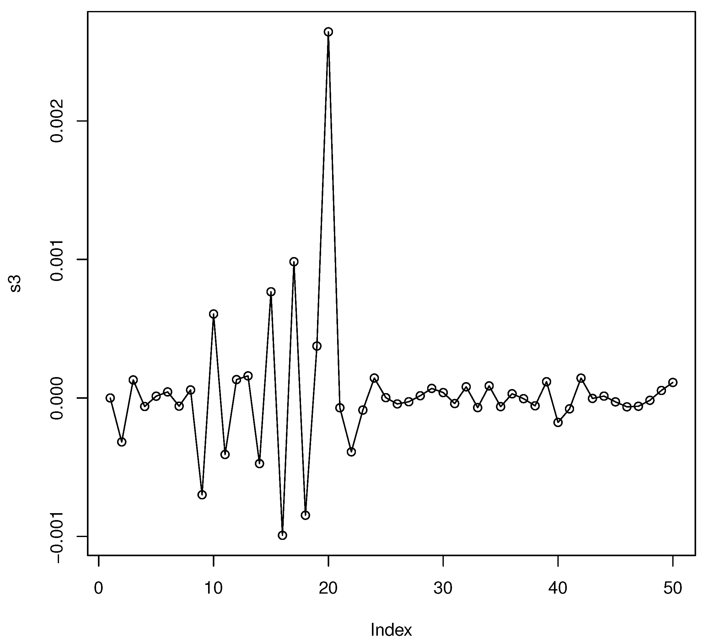
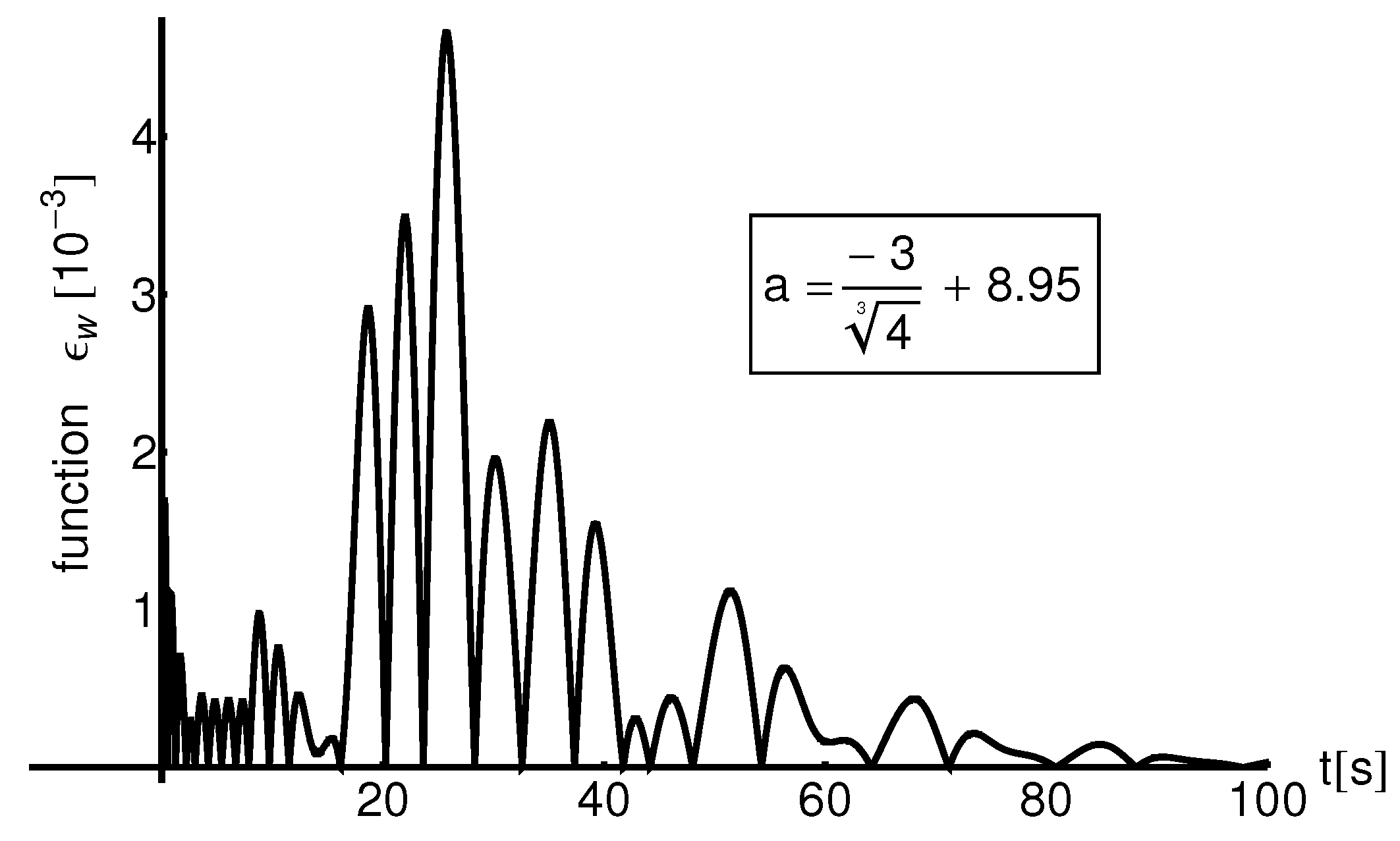
4.1. Qualitative Analysis of Errors

The primary issue in more dynamic systems is that precise solutions are not available. To achieve approximate solutions, one relies on observations or data collected from physical phenomena, or on numerical solutions or simulations.

In such cases, the so-called “errors” in fact reflect the discrepancies between the approximate solutions and certain numerical values obtained from a numerical method. Therefore, it is more accurate to refer to these discrepancies as “residuals”. Conducting a qualitative analysis of these residuals appears to hold significant importance.

In the fields of statistics and optimization, errors refer to the theoretical, unobservable discrepancies between an observed value and the true model, which represents the exact solution in a given context. In contrast, residuals are the measurable, calculated differences between an observed value and the estimated or predicted value derived from a sample model, which serves as an approximate solution.

Errors are random, while residuals are used to estimate these unknown error (see Cox et al. [34]).

Many methods that provide approximate solutions only present the residual values and limit themselves to stating that the method is good if these residual values are, in absolute value, very small, without making a qualitative study of the series of residual values. In general, these methods claim to be efficient if they have a low computational time, which is no longer a real problem today when the computing power of computers has increased greatly.

The main purpose of the statistical analysis of the series of residual values was to verify whether or not there is any relation, deterministic, between the values in this series. If there is no deterministic relationship between these values, it can be concluded that the series of residual values (that is, the series of differences between the approximate solution and the numerical solution with Runge–Kutta) really represents a series of errors.

To answer the question related to a possible connection between the residual values, known statistical methods are applied that study possible connections between the values of the series, more precisely the correlation between the values of the residual series is studied. Appropriate statistical tests are applied for this purpose. If a correlation is found between the values of the series, this suggests a deterministic relationship between the values, which may be due to the fact that the approximate solution is not the best mathematical, deterministic expression to describe the dynamic system studied. If it is not possible to support, statistically, a connection between the values of the residual series, it can be stated that the approximate solution is good, it approaches the numerical solution very well, and the residual values are only errors due to approximation.

Most used techniques are oriented to check three aspects:

First, the residuals should exhibit a constant mean value, which is typically close to zero in most approximate solutions. More importantly, they should maintain a constant variance, a property commonly referred to as homoscedasticity.

Second, the residuals must be uncorrelated (or show no autocorrelation). This aspect is crucial for determining whether there are any periodic patterns or trends within the residual series. Ensuring this lack of correlation supports the idea that the approximate solution is the most accurate analytical representation of the behavior of the associated dynamical system.

Third, it is necessary to verify if the empirical distribution of the residuals closely resembles a known theoretical probability distribution. In most cases, this distribution is expected to follow a normal, or Gaussian, distribution.

It is known that a nonnormal probability distribution (nonGauss–Laplace) is not necessarily wrong. Nonnormality can occur if the volume of data is small, if there are extreme values (outliers), if there are systematic errors, etc. (in the present case, outliers are found, as can be seen in the box-plot graph). There are probability distributions that approach the normal one, such as the Student distribution (t-distribution) or other distributions with heavy tails (e.g., stable distributions) that are often found in the real world and that do not necessarily suggest something serious in the series of values. It is important that the values from different groups of the residual series follow the same probability distribution.

Each of the aspects mentioned can be analyzed using suitable statistical tests, many of which are available through open-source or free software, such as R or RStudio, version 4.5.0.

Additionally, graphical representations can assist in making straightforward observations about the residuals’ pattern, for instance, simple 2D plots or histograms.

All calculations for these statistical tests were conducted using R software, version 4.5.0.

We divided our data into three groups (the length of series is 50), i.e., $[1,17]$, $[18,36]$ and $[37,50]$.

Graphical representation (see Figure 6 and Figure 7):

4.2. Study of Heteroscedasticity

Results for our example:

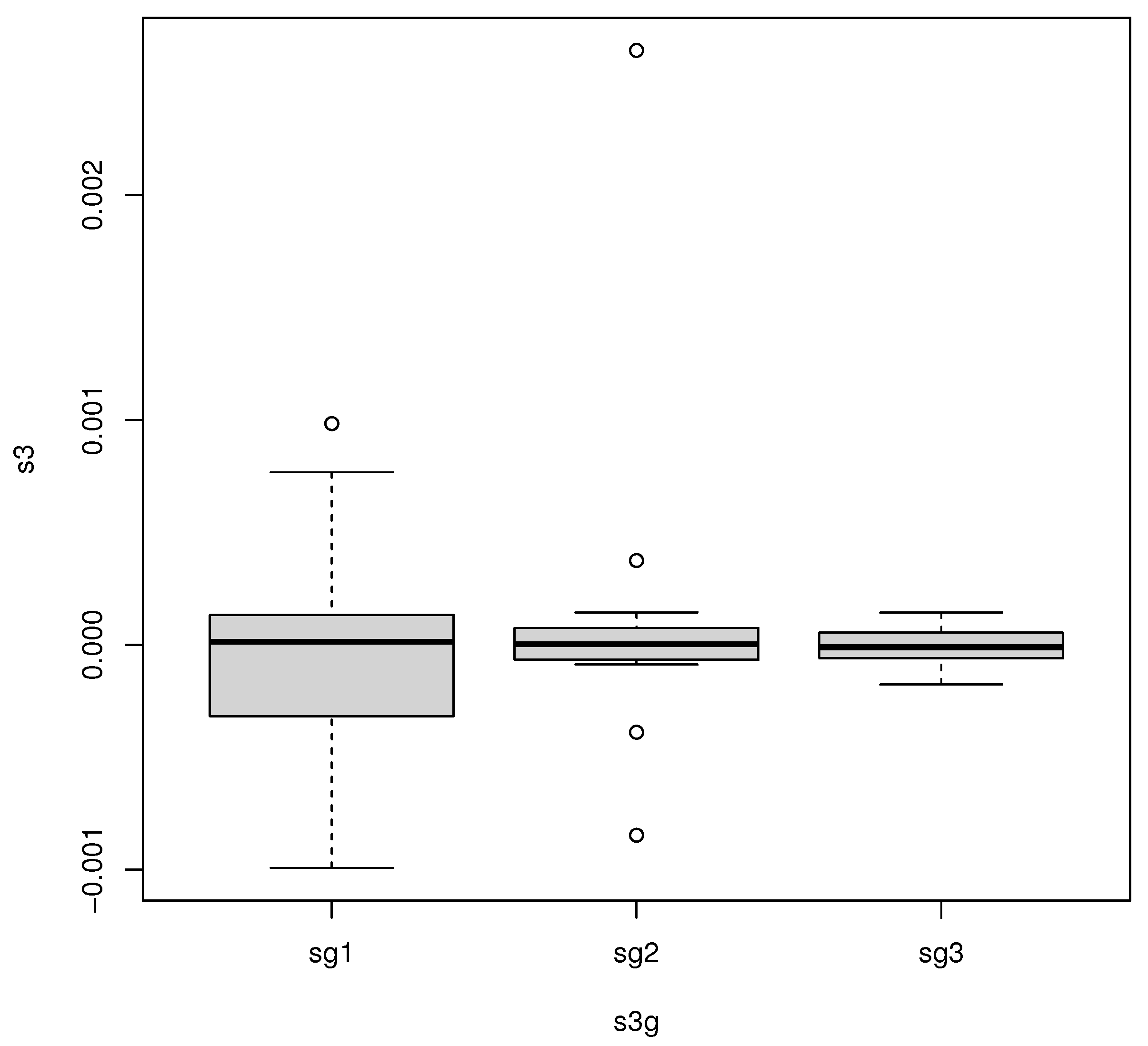
• First, the box-plot graph (see Figure 8):

  Figure 8. Box-plot for residuals.

  Figure 8. Box-plot for residuals.
• Second, the statistical mean value and, respectively, the standard deviation: Mean value of groups

  $$\begin{array}{ccccc}subgroup& & sg1& sg2& sg3\\ mean& & -6.809178\times {10}^{-6}& 9.741967\times {10}^{-5}& -3.455164\times {10}^{-6}\end{array}$$
  Standard deviation of groups

  $$\begin{array}{ccccc}subgroup& & sg1& sg2& sg3\\ st.deviation& & 4.975618\times {10}^{-4}& 6.618851\times {10}^{-4}& 8.732643\times {10}^{-5}\end{array}$$
• The Bartlett test in R
  Null Hypothesis ($H_0$): All group variances are equal.
  Alternative Hypothesis ($H_a$): At least two group variances are different.
  For each of ${\displaystyle i\in \{1,\dots ,k\}}$, take ${\displaystyle n_i}$ samples from that population. Let its sample variances be ${\displaystyle S_i^2}$. Bartlett’s test statistic is

  $${\displaystyle {\chi }^2=\frac{(N-k)ln\left(S_p^2\right)-{\displaystyle \sum _{i=1}^k}(n_i-1)ln\left(S_i^2\right)}{1+\frac{1}{3(k-1)}\left({\displaystyle \sum _{i=1}^k}\left(\frac{1}{n_i-1}\right)-\frac{1}{N-k}\right)}}$$

  where ${\displaystyle N=\sum _{i=1}^k{n}_i}$ and ${\displaystyle S_p^2=\frac{1}{N-k}\sum _i(n_i-1)S_i^2}$ is the pooled estimate for the variance (see Bartlett [35]).
  Results from R-software:
  Bartlett’s K-squared = 35.186, df = 2, p-value = 2.288 $\times {10}^{-8}$
  Since the p-value is less than 0.05, the decision is to reject $H_0$, indicating that the data is consistent with unequal variances from a statistical perspective. However, this classical test has certain limitations, particularly when the values in the series (residuals) are not normally distributed (as explained in Section 3) or when outliers whether accidental, atypical, or abnormal are present. Over time, alternative tests have been proposed to assess homoscedasticity, such as Levene’s Test for Homogeneity of Variance.
• The Levene’s test in R
  Levene’s test is an inferential statistical method used to evaluate whether the variances of a variable are equal across two or more groups. The test examines the null hypothesis, which posits that population variances are equal to a condition known as homogeneity of variance or homoscedasticity. When the test generates a p-value lower than a predetermined significance level, typically 0.05, it suggests that the observed differences in sample variances are unlikely to be due to random sampling from a population with equal variances. Consequently, the null hypothesis of equal variances is rejected, indicating that the variances in the population differ.
  The test statistic,

  $${\displaystyle W=\frac{(N-k)}{(k-1)}·\frac{{\displaystyle \sum _{i=1}^k}{N}_i{(Z_{i·}-Z_{··})}^2}{{\displaystyle \sum _{i=1}^k}{\displaystyle \sum _{j=1}^{N_i}}{(Z_{ij}-Z_{i·})}^2},}$$

  where:
  k is the number of different groups to which the sampled cases belong,
  ${\displaystyle N_i}$ is the number of cases in the ${\displaystyle i}$-th group,
  N is the total number of cases in all groups,
  ${\displaystyle Y_{ij}}$ is the value of the measured variable for the ${\displaystyle j}$-th case from the ${\displaystyle i}$-th group,
  ${\displaystyle Z_{ij}=\left\{\begin{array}{cc}|Y_{ij}-{\overline{Y}}_{i·}|,& {\overline{Y}}_{i·} \mathrm{is} \mathrm{a} \mathrm{mean} \mathrm{of} \mathrm{the} i-\mathrm{th} \mathrm{group},\\ |Y_{ij}-{\tilde{Y}}_{i·}|,& {\tilde{Y}}_{i·} \mathrm{is} \text{a} \mathrm{median} \mathrm{of} \mathrm{the} i-\mathrm{th} \mathrm{group}.\end{array}\right.}$
  (both definitions are in use)
  ${\displaystyle Z_{i·}=\frac{1}{N_i}\sum _{j=1}^{N_i}{Z}_{ij}}$ is the mean of the ${\displaystyle Z_{ij}}$ for group i,
  ${\displaystyle Z_{··}=\frac{1}{N}\sum _{i=1}^k\sum _{j=1}^{N_i}{Z}_{ij}}$ is the mean of all ${\displaystyle Z_{ij}}$,
  (see [36,37]).
  Results from the R-software:
  Df F value $Pr(>F)$
  47 1.7343 0.1876
  Because the p-value > 0.05, then the decision is “fails to reject the null hypothesis”, i.e., “The assumption of equal variances (homoscedasticity) holds true”.

4.3. Study of Autocorrelation

Results for our example:

• Durbin–Watson test
  The Durbin–Watson statistic serves as a diagnostic tool to identify autocorrelation at lag 1 within the residuals (prediction errors) of a regression analysis. Autocorrelation arises when residuals are not independent, thus breaching a fundamental assumption of linear regression. This test is specifically designed to uncover potential patterns or relationships in the errors over time or across observations.
  If $e_i$ is the residual series, then

  $${\displaystyle DW=\frac{{\displaystyle \sum _{i=2}^N}{(e_i-e_{i-1})}^2}{{\displaystyle \sum _{i=1}^N}{e}_i^2},}$$

  where N is the number of observations. For large N, $DW$ is approximately equal to $2(1-\widehat{\rho })$, where ${\displaystyle \widehat{\rho }}$ is the sample autocorrelation of the residuals at lag 1 (see Durbin et al. [38]).
  This test is designed to evaluate the following statistical hypotheses:
  Null Hypothesis (H₀): there is no first-order autocorrelation present in the residuals.
  Alternative Hypothesis (H_a): first-order autocorrelation exists in the residuals.
  For making a statistical decision, a p-value less than 0.05 indicates significant evidence of autocorrelation, justifying the rejection of the null hypothesis that assumes uncorrelated residuals. Additionally, in cases where autocorrelation is detected, some common interpretations or implications may arise regarding model adequacy and potential adjustments needed for improved accuracy.
  $DW\approx 2$: residuals are likely independent (no autocorrelation).
  $DW<2$: suggests positive autocorrelation, common in time-series data.
  $DW>2$: suggests negative autocorrelation
  In practice, a value near 2 indicates no autocorrelation, while values closer to 0 indicate positive correlation, and values closer to 4 indicate negative correlation. Generally, values of 1.5–2.5 are considered acceptable (see, for example Field [39]). More precisely, to make a precise decision, compare the calculated statistic $DW$ to the lower $D{W}_L$ and upper $D{W}_U$ critical values from a Durbin–Watson table (see, for example, https://real-statistics.com/statistics-tables/durbin-watson-table/, accessed on 15 February 2026), both values depend on N, the number of observations. The decision is one of the following:
  Reject “Positive Autocorrelation” if $DW<D{W}_L$
  Reject “Negative Autocorrelation” if $DW>4-D{W}_L$ or $DW>4-D{W}_U$
  “No Autocorrelation” if $D{W}_U<DW<4-D{W}_U$,
  “Inconclusive” if $D{W}_L<DW<D{W}_U$ or $4-D{W}_L<DW<4-D{W}_U$.
  For our case, i.e., $N=50$ and $\alpha =0.05$, we have the limits $D{W}_L=1.50$ and $D{W}_U=1.59$
  The null hypothesis ($H_0$) asserts that there is no first-order autocorrelation in the residuals, while the alternative hypothesis ($H_a$) posits the existence of first-order autocorrelation.
  For statistical decision-making, a p-value below 0.05 indicates significant autocorrelation, warranting the rejection of the null hypothesis that residuals are uncorrelated.

  -

  DW ≈ 2: Residuals are likely independent, indicating no autocorrelation.

  -

  DW < 2: Implies positive autocorrelation, which is commonly observed in time-series data.

  -

  DW > 2: Suggests negative autocorrelation.

  Additionally, the Durbin–Watson (DW) statistic provides insights into the degree of autocorrelation:

  -

  DW ≈ 2: residuals are likely independent, indicating no autocorrelation;

  -

  DW < 2: implies positive autocorrelation, which is commonly observed in time-series data;

  -

  DW > 2: suggests negative autocorrelation

  Results from the R-software:
  DW = 2.6161, p-value = 0.9751
  We have that the p-value > 0.05, hence, the statistical decision is “fails to reject the null hypothesis”.

4.4. Study of Normality

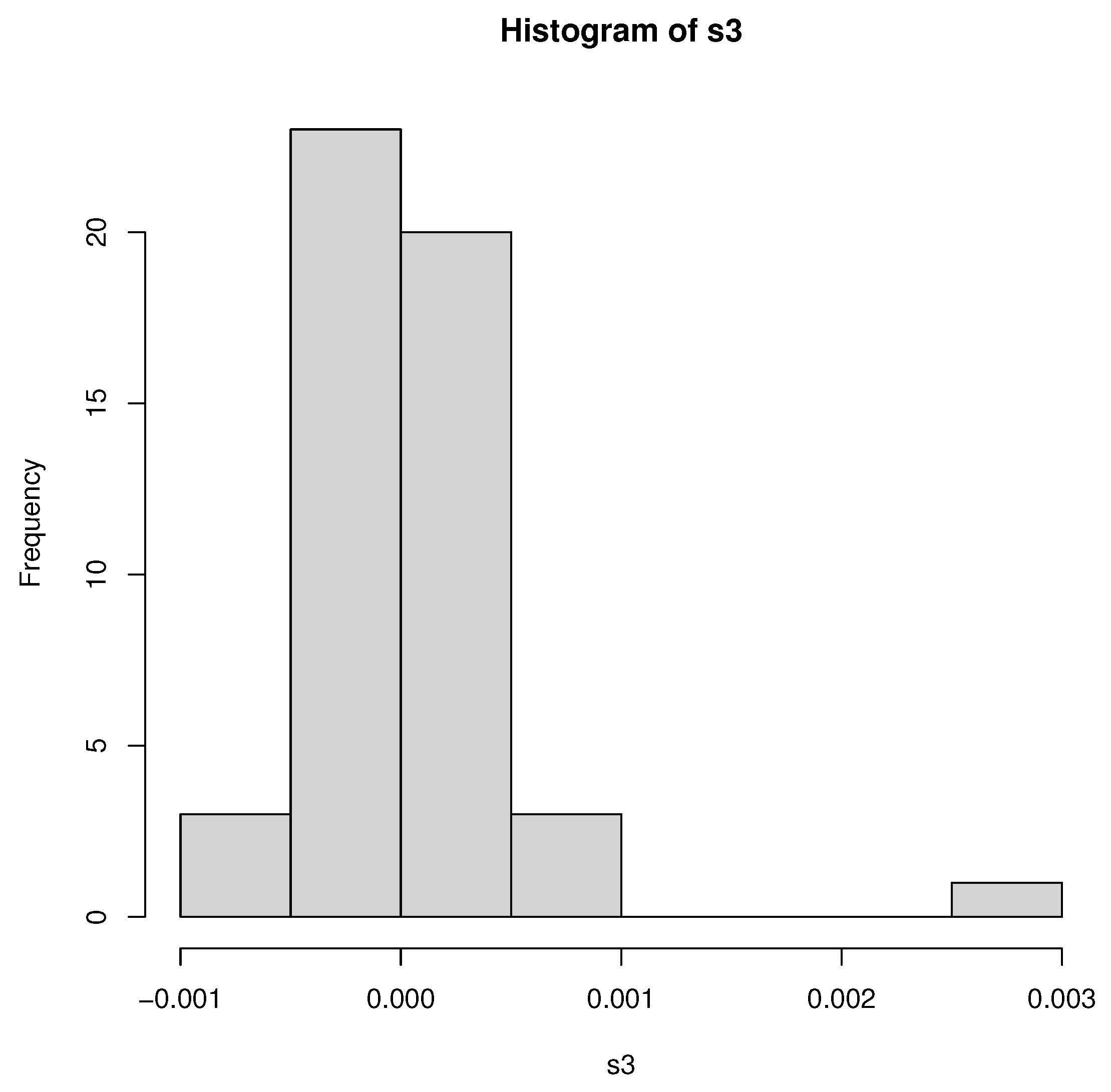
• Shapiro–Wilk test
  The Shapiro–Wilk test is a test of normality (see Shapiro et al. [40]). The Shapiro–Wilk test tests the null hypothesis that a sample $x_1$, …, $x_n$ came from a normally distributed population. The test statistic is

  $${\displaystyle W=\frac{{\left({\displaystyle \sum _{i=1}^n}{a}_i{x}_{\left(i\right)}\right)}^2}{{\displaystyle \sum _{i=1}^n}{\left(x_i-\overline{x}\right)}^2},}$$

  where ${\displaystyle x_{\left(i\right)}}$ with parentheses enclosing the subscript index i is the ith order statistic, i.e., the ith-smallest number in the sample (not to be confused with ${\displaystyle x_i})$,
  ${\displaystyle \overline{x}=\left(x_1+\dots +x_n\right)/n}$ is the sample mean.
  The coefficients ${\displaystyle a_i}$ are given by:

  $${\displaystyle (a_1,\dots ,a_n)=\frac{m^{\mathsf{T}}{V}^{-1}}{C},}$$

  where C is a vector norm, i.e., ${\displaystyle C=∥V^{-1}m∥={\left(m^{\mathsf{T}}{V}^{-1}{V}^{-1}m\right)}^{1/2}}$ and the vector ${\displaystyle m={(m_1,\dots ,m_n)}^{\mathsf{T}}}$ represents the expected values of the order statistics derived from independent and identically distributed random variables sampled from a standard normal distribution. Additionally, V denotes the covariance matrix associated with these normal order statistics.
  The null hypothesis for this test posits that the population follows a normal distribution. If the calculated p-value is smaller than the predetermined significance level (alpha), the null hypothesis is rejected, indicating evidence that the tested data deviates from normality. Results for our data:
  W = 0.67334, p-value = 2.835 $\times {10}^{-9}$
  In this case, the p-value < 0.05, then a decision can be “to reject $H_0$”, i.e., “data is significantly non-normal”.
• Kolmogorov–Smirnov test
  The Kolmogorov–Smirnov test can be adapted for use as a goodness-of-fit test. Specifically, when assessing the normality of a distribution, the samples are first standardized and then compared to a standard normal distribution.
  This approach essentially involves aligning the mean and variance of the reference distribution with the sample estimates. However, it is well established that defining the specific reference distribution in this manner alters the null distribution of the test statistic (see Kolmogorov [41] and Smirnov [42]).
  The empirical distribution function $F_n$, corresponding to n independent and identically distributed (i.i.d.) ordered observations $X_i$, is defined as follows:

  $${\displaystyle F_n\left(x\right)=\frac{\mathrm{number} \mathrm{of} (\mathrm{elements} \mathrm{in} \mathrm{the} \mathrm{sample}\le x)}{n}=\frac{1}{n}\sum _{i=1}^n{1}_{(-\infty ,x]}\left(X_i\right),}$$

  where ${\displaystyle 1_{(-\infty ,x]}\left(X_i\right)}$ is the indicator function, equal to ${\displaystyle X_i\le x}$ and equal to 0 otherwise.
  The Kolmogorov–Smirnov statistic for a given cumulative distribution function $F\left(x\right)$ is

  $${\displaystyle D_n=\underset{x}{sup}|F_n\left(x\right)-F\left(x\right)|}.$$
  The supremum, or $sup$, represents the maximum value within the set of distances. Essentially, this statistic identifies the greatest absolute difference between the two distribution functions over all possible x values.
  Output from R software:
  D = 0.29989, p-value = 0.0001748
  The p-value > 0.05, hence, the statistical decision is “to reject the null hypothesis of normality”.
  The Kruskal–Wallis test is a nonparametric, or distribution-free, statistical test designed for situations where the assumptions of one-way ANOVA are not satisfied. Both tests are used to compare a continuous dependent variable across multiple groups. Unlike ANOVA, which requires the dependent variable to follow a normal distribution and exhibit equal variance across groups, the Kruskal–Wallis test does not rely on these assumptions.
  One key advantage of the Kruskal–Wallis test is its flexibility, as it can be applied to both continuous and ordinal-level dependent variables. However, similar to many nonparametric tests, it tends to be less powerful than ANOVA when the assumptions of ANOVA are met.
  The hypotheses for the Kruskal–Wallis test are as follows:

  -

  Null hypothesis: the samples (groups) are drawn from identical populations.

  -

  Alternative hypothesis: at least one sample (group) comes from a population that differs from the others.

  Output form R for our data
  Kruskal–Wallis chi-squared $=0.10969$, $df=2$, p-value = 0.9466,
  hence, with great probability, we cannot reject the null hypothesis.

5. Conclusions

This paper is dedicated to building exact parametric solutions for one 3D dynamic system, depending on a physical parameter, but which does not admit the Hamilton–Poisson structure. The system admits a single equilibrium point that could be integrated explicitly, via a smooth function.

An analytical approach, OAFM, for solving nonlinear differential equations is presented using only one iteration. The obtained results are validated by graphical comparison with the corresponding numerical solutions. The precision of the obtained OAFM results is investigated qualitatively and quantitatively by means of the statistical tests of residuals. A rigorous analysis of errors is provided by highlighted heteroscedasticity, autocorrelation, and normality.

The accuracy of the obtained results encourages the study of other dynamical systems usefully in many technological applications based on periodically or damped oscillations behavior.

References

- Deng, K.; Yu, S. Estimating ultimate bound and finding topological horseshoe for a new chaotic system. Optik 2014, 125, 6044–6048. [Google Scholar] [CrossRef]
- Rameshbabu, R. Dynamic Analysis of a New Chaotic System with Multistability, Amplitude and Offset Boosting Control, Its Adaptive Synchronization. In Proceedings of the 2nd International Conference on Nonlinear Dynamics and Applications (ICNDA 2024); Springer: Cham, Switzerland, 2024; Volume 1, pp. 654–667. [Google Scholar]
- Suneja, K.; Garg, A.; Sharma, A.; Yash, A. A novel Three-Key mixing text encryption based on A new 3-D chaotic system. Analog Integr. Circ. Signal Process. 2025, 125, 48. [Google Scholar] [CrossRef]
- Liu, H. Audio block encryption using 3D chaotic system with adaptive parameter perturbation. Multimed. Tools Appl. 2023, 82, 27973–27987. [Google Scholar] [CrossRef]
- Ye, X.; Wang, X. Hidden oscillation and chaotic sea in a novel 3D chaotic system with exponential function. Nonlinear Dyn. 2023, 111, 15477–15486. [Google Scholar] [CrossRef]
- Wang, S. A 3D autonomous chaotic system: Dynamics and synchronization. Indian J. Phys. 2024, 98, 4525–4533. [Google Scholar] [CrossRef]
- Gao, X.; Wang, Y. The Sprott K chaotic oscillator for image encryption. Indian J. Phys. 2025, 11. [Google Scholar] [CrossRef]
- Zhou, Z.; Zhao, B.; Ye, X. Generating rotationally multi-scroll attractive sea via a novel 3D chaotic system with two memristors. Eur. Phys. J. Plus 2023, 138, 674. [Google Scholar] [CrossRef]
- Yang, H.; Liu, Y.; Li, G. Analysis of 3D chaotic system with novel double scroll structure and additional nonlinear functions and its application in weak signal detection. Eur. Phys. J. Plus. 2025, 140, 637. [Google Scholar] [CrossRef]
- Khattar, D.; Agrawal, N.; Singh, G. Chaotic Analysis of a New 3D System with Exponential Nonlinearity and its Dual Compound Combination Multiswitching Synchronization using Nonlinear Control. Int. J. Appl. Comput. Math. 2025, 11, 98. [Google Scholar] [CrossRef]
- Wang, J.; Dong, C.; Li, H. A New Variable-Boostable 3D Chaotic System with Hidden and Coexisting Attractors: Dynamical Analysis, Periodic Orbit Coding, Circuit Simulation, and Synchronization. Fractal Fract. 2022, 6, 740. [Google Scholar] [CrossRef]
- Stroita, D.C.; Bordeasu, D.; Dragan, F. System Identification of a Servo-Valve Controlled Hydraulic Cylinder Operating Under Variable Load. Mathematics 2025, 13, 341. [Google Scholar] [CrossRef]
- Khairudin, M. Dynamic analysis and modeling of three-dimensional crane incorporating payload. J. Phys. Conf. Ser. 2020, 1446, 012003. [Google Scholar] [CrossRef]
- Gholamin, P.; Refahi Sheikhani, A.H. A new three-dimensional chaotic system: Dynamical properties and simulation. Chin. J. Phys. 2017, 55, 1300–1309. [Google Scholar] [CrossRef]
- Tong, Y.-N. Dynamics of a three-dimensional chaotic system. Optik 2015, 126, 5563–5565. [Google Scholar] [CrossRef]
- Deng, K.-b.; Wang, R.-X.; Li, C.-L.; Fan, Y.-Q. Tracking control for a ten-ring chaotic system with anexponential nonlinear term. Optik 2017, 130, 576–583. [Google Scholar] [CrossRef]
- Puta, M. Integrability and geometric prequantization of the Maxwell-Bloch equations. Bull. Sci. Math. 1998, 122, 243–250. [Google Scholar] [CrossRef][Green Version]
- Ene, R.-D.; Pop, N.; Badarau, R. Closed-Form Solutions for a Dynamical System Using Optimal Parametric Iteration Method. Axioms 2026, 15, 1. [Google Scholar] [CrossRef]
- Ene, R.-D.; Pop, N.; Badarau, R. Semi-Analytical Solutions for the Qi-Type Dynamical System. Symmetry 2024, 16, 1578. [Google Scholar] [CrossRef]
- Ene, R.-D.; Pop, N. Semi-Analytical Closed-Form Solutions for the Rikitake-Type System through the Optimal Homotopy Perturbation Method. Mathematics 2023, 11, 78. [Google Scholar] [CrossRef]
- Marinca, V.; Herisanu, N.; Marinca, B. Approximate Solution to Nonlinear Dynamics of a Piezoelectric Energy Harvesting Device Subject to Mechanical Impact and Winkler-Pasternak Foundation. Materials 2025, 18, 1502. [Google Scholar] [CrossRef]
- Iqbal, A.; Nawaz, R.; Ashraf, R.M.; Fewster-Young, N.H. Extension of optimal auxiliary function method to nonlinear Sin Gordon partial differential equations. Partial Differ. Equ. Appl. Math. 2024, 10, 100735. [Google Scholar] [CrossRef]
- Alshehry, A.; Yasmin, H.; Ahmad, M.; Khan, A.; Shah, R. Optimal Auxiliary Function Method for analyzing nonlinear system of Belousov-Zhabotinsky Equation with Caputo operator. Axioms 2023, 12, 825. [Google Scholar] [CrossRef]
- Alshehry, A.; Yasmin, H.; Ganie, A.; Ahmad, M.; Shah, R. Optimal auxiliary function method for analyzing nonlinear system of coupled Schrödinger–KdV equation with Caputo operator. Open Phys. 2023, 21, 20230127. [Google Scholar] [CrossRef]
- Mohammadian, M. Approximate analytical solutions to nonlinear damped oscillatory systems using a modified algebraic method. J. Appl. Mech. Tech. Phys. 2021, 62, 70–78. [Google Scholar] [CrossRef]
- Liu, C.S.; Kuo, C.L.; Chang, C.W. Linearized Harmonic Balance method for seeking the periodic vibrations of second- and third-order nonlinear oscillators. Mathematics 2025, 13, 162. [Google Scholar] [CrossRef]
- Aljahdaly, N.H.; Alharbi, M.A.; El-Tantavy, S.A. On the oscillations in a nonextensive complex plasma by improved differential transformation method: An application to a damped Duffing equation. J. Low Freq. Noise Vib. Act. Control 2023, 42, 1319–1327. [Google Scholar] [CrossRef]
- Ullah, H.; Islam, S.; Khan, I.; Shafie, S.; Fiza, M. Formulation and application of Optimal Homotopy Asymptotic Method to coupled differential-difference equations. PLoS ONE 2015, 10, e0120127. [Google Scholar] [CrossRef]
- Nicoara, A.; Stoia, D.I.; Chilibaru-Opritescu, C.; Herisanu, N. A biodynamic multibody system. OHAM solution. AIP Conf. Proc. 2022, 2425, 310007. [Google Scholar] [CrossRef]
- Hu, C.; Tian, Z.; Wang, Q.; Zhang, X.; Liang, B.; Jian, C.; Wu, X. A memristor-based VB2 chaotic system: Dynamical analysis, circuit implementation, and image encryption. Optik 2022, 269, 169878. [Google Scholar] [CrossRef]
- Marinca, V.; Herisanu, N. Approximate analytical solutions to Jerk equation. In Springer Proceedings in Mathematics & Statistics: Proceedings of the Dynamical Systems: Theoretical and Experimental Analysis, Lodz, Poland, 7–10 December 2015; Springer: Cham, Switzerland, 2016; Volume 182, pp. 169–176. [Google Scholar]
- Marinca, V.; Ene, R.-D.; Marinca, V.B. Optimal Auxiliary Functions Method for viscous flow due to a stretching surface with partial slip. Open Eng. 2018, 8, 261–274. [Google Scholar] [CrossRef]
- Ene, R.-D.; Pop, N.; Lapadat, M.; Dungan, L. Approximate closed-form solutions for the Maxwell-Bloch equations via the Optimal Homotopy Asymptotic Method. Mathematics 2022, 10, 4118. [Google Scholar] [CrossRef]
- Cox, D.R.; Snell, E.J. A general definition of residuals. J. R. Stat. Soc. Ser. B 1968, 30, 248–265. [Google Scholar] [CrossRef]
- Bartlett, M.S. Properties of sufficiency and statistical tests. Proc. R. Stat. Soc. Ser. A 1937, 160, 268–282. [Google Scholar] [CrossRef]
- Levene, H. Robust tests for equality of variances. In Contributions to Probability and Statistics; Olkin, I., Ed.; Stanford University Press: Palo Alto, CA, USA, 1960. [Google Scholar]
- Olkin, I.; Ghurye, S.G.; Hoeffding, W.; Madow, W.G.; Mann, H.B. (Eds.) Contributions to Probability and Statistics: Essays in Honor of Harold Hotelling; Stanford University Press: Palo Alto, CA, USA, 1960; pp. 278–292. [Google Scholar]
- Durbin, J.; Watson, G.S. Testing for Serial Correlation in Least Squares Regression. III. Biometrika 1971, 58, 1–19. [Google Scholar] [CrossRef]
- Field, A. Discovering Statistics Using SPSS, 3rd ed.; Sage Publications: Newcastle upon Tyne, UK, 2009. [Google Scholar]
- Shapiro, S.S.; Wilk, M.B. An analysis of variance test for normality (complete samples). Biometrika 1965, 52, 591–611. [Google Scholar] [CrossRef]
- Kolmogorov, A. Sulla determinazione empirica di una legge di distribuzione. G. Ist. Ital. Attuari. 1933, 4, 83–91. [Google Scholar]
- Smirnov, N. Table for estimating the goodness of fit of empirical distributions. Ann. Math. Stat. 1948, 19, 279–281. [Google Scholar] [CrossRef]