A New Perspective on the Energy Decay of the Timoshenko–Ehrenfest System: The Non-Local Truncated Approach

Abstract

This paper presents a new perspective on the energy decay of a nonlocal truncated Timoshenko–Ehrenfest system. By using the non local elasticity theory, this model is a generalization of the standard truncated Timoshenko system. The well-posedness of the proposed model is established via the Faedo-Galerkin method. Energy stability and decay properties are then derived using suitable multiplier techniques. Finally, a numerical scheme is constructed, and the exponential decay of the discrete energy is given special attention. Numerical simulations are provided to illustrate and validate the theoretical results.

1. Introduction

In the framework of continuum mechanics, broad research has been undertaken to explore the mechanical proporeties of elastic and viscoelastic beam models. The most commonly used are the classical Euler–Bernoulli and Timoshenko beam models. An essential aspect of structural modeling is the consideration of scale effects. While classical continuum theories are widely employed due to their computational efficiency, their ability to accurately represent small-scale phenomena in mechanical behavior remains limited. Extensive studies have emphasized the critical role of scale effects and demonstrated that nonlocal elastic continuum theories provide a more reliable framework for predicting structural responses. The origins of nonlocal elasticity theory lie in the pioneering investigations conducted by Eringen [1,2] and Reddy [3]. In [3], Reddy employs nonlocal constitutive differential equations to formulate classical beam and shear deformation theories rigorously and to derive analytical solutions for bending, buckling, and natural frequency problems of simply supported beams.

The Timoshenko system (see [4]) is written as,

$$\begin{array}{cc}\hfill & {\rho }_1{\varphi }_{tt}(x,t)=S_x(x,t),\hfill \\ \hfill & {\rho }_2{\psi }_{tt}(x,t)=M_x(x,t)-S(x,t),\hfill \end{array}$$

(1)

where $(x,t)\in (0,L)\times (0,\infty )$, t is the time, x is the distance along the center line of the beam structure, L is the length of the beam, $\varphi$ is the transverse displacement, and $\psi$ is the rotation of the neutral axis due to bending. Here, ${\rho }_1=\rho A$ and ${\rho }_2=\rho I$, where $\rho >0$ is the density, A is the cross-sectional area, and I is the second moment of the cross-sectional area. By S, we denote the shear force, and M is the bending moment. The constitutive laws are given by (see [4])

$$\begin{array}{cc}\hfill & S=k({\varphi }_x+\psi ),\hfill \\ \hfill & M=b{\psi }_x.\hfill \end{array}$$

(2)

Here, b and k stand for $b=EI$ and $k=k_{1}GA$ where E, G, and $k_1$ represent Young’s modulus, the modulus of rigidity, and the transverse shear factor, respectively.

Substituting Equation (2) in (1), we get the Timoshenko system

$$\left\{\begin{array}{cc}\hfill & {\rho }_1{\varphi }_{tt}-k{({\varphi }_x+\psi )}_x=0,\hspace{1em}\mathrm{in}\hspace{1em}(0,L)\times (0,\infty ),\hfill \\ \hfill & {\rho }_2{\psi }_{tt}-b{\psi }_{xx}+k{({\varphi }_x+\psi )}_x=0,\hspace{1em}\mathrm{in}\hspace{1em}(0,L)\times (0,\infty ).\hfill \end{array}\right.$$

(3)

Soufyane [5] established a necessary and sufficient condition for exponential stability of the linear Timoshenko beam with frictional damping. He proved that the total energy decays exponentially if and only if the stability number $\chi =k/{\rho }_1-b/{\rho }_2$ vanishes, which corresponds to the equality of the wave propagation speeds of the system. In [6] Malacarne and Rivera showed that the viscoelastic Timoshenko system is not exponentially stable.

In the framework of Eringen’s nonlocal elasticity [1,2], the stress at a given point of a continuum does not depend solely on the strain at that point, as in classical elasticity, but rather on the strain field in its entire neighborhood. In its integral form, the constitutive relation can be written as

$$\sigma \left(x\right)={\int }_{\mathsf{\Omega }}\alpha \left(\right|x-\xi \left|\right)\epsilon \left(\xi \right)d\xi ,$$

where $\alpha \left(\right|x-\xi \left|\right)$ is a nonlocal attenuation kernel that characterizes the influence of the strain at the point $\xi$ on the stress at x.

For practical applications, Eringen showed that this integral model is equivalent, under appropriate assumptions on the kernel, to the following differential form:

$$(1-{\mu }^2{\partial }_{xx})\sigma =E\epsilon ,$$

where $\mu$ is the nonlocal parameter that introduces a material length scale.

In the context of the Timoshenko–Ehrenfest beam model, this differential nonlocal formulation is applied to the bending moment M and the shear force S, yielding

$$\left(1-{\mu }^2{\partial }_{xx}\right)M=b{\psi }_x,\hspace{1em}\hspace{1em}\left(1-{\mu }^2{\partial }_{xx}\right)S=k\left({\varphi }_x+\psi \right),$$

(4)

where ${\mu }^2$ is the nonlocal parameter.

Applying the operator $\left(1-{\mu }^2{\partial }_{xx}\right)$ to the balance equations and using the nonlocal constitutive relations, we obtain the non-local Timoshenko–Ehrenfest system

$$\left\{\begin{array}{cc}\hfill & {\rho }_1{\varphi }_{tt}-{\mu }^2{\rho }_1{\varphi }_{ttxx}-k{\left({\varphi }_x+\psi \right)}_x=0,\hfill \\ \hfill & {\rho }_2{\psi }_{tt}-{\mu }^2{\rho }_2{\psi }_{ttxx}-b{\psi }_{xx}+k\left({\varphi }_x+\psi \right)=0.\hfill \end{array}\right.$$

(5)

The Timoshenko–Ehrenfest system has important physical significance because it provides a more realistic description of beam vibrations compared to the classical Euler–Bernoulli theory. In practical engineering structures such as short beams, thick beams, bridges, aircraft wings, and mechanical components, both shear deformation and rotary inertia play a significant role. The Timoshenko–Ehrenfest model accounts for these effects by coupling the transverse displacement with the rotation of the cross-section, allowing it to accurately predict bending behavior, vibration frequencies, and dynamic responses. This makes the system especially important in modern structural engineering, materials science, and vibration control, where precise modeling of elastic structures is essential for safety and performance.

A particular vibrational regime, known as the second spectrum of frequency, influences the Timoshenko system and is intrinsic to the analysis of Timoshenko beam theory. The two propagation velocities are inversely proportional for small wave numbers, with one phase velocity becoming unbounded at low frequencies. This striking physical behavior may be attributed to the influence of the second spectrum [7]. To circumvent the detrimental effects associated with the second spectrum, Elishakoff’s technique [8] is employed to derive a truncated Timoshenko system. This approach consists of replacing the term ${\psi }_{tt}$ with $-{\varphi }_{ttx}$, in accordance with d’Alembert’s principle of dynamic equilibrium. This eliminates the second spectrum of frequency and its damaging effects on wave propagation speed. Almeida et al. [7] established a link between the phenomenon known as the second spectrum of frequency, often regarded as non-physical or associated with modeling inconsistencies, and the exponential decay behavior exhibited by dissipative Timoshenko systems. Commonly arising in stabilization analyses, the second spectrum can be effectively suppressed through the incorporation of damping mechanisms into the classical Timoshenko model. Moreover, they proved that dissipative Timoshenko systems devoid of the second spectrum are exponentially stable for arbitrary values of the system coefficients.

The truncated Timoshenko system has attracted the interest of many researchers because recent studies have shown that systems exhibiting a second spectrum generally fail to achieve exponential energy decay unless the wave speeds are equal. Without this restrictive assumption, only polynomial decay is obtained, which is often of limited practical relevance for engineering applications. In contrast, the truncated systems typically exhibit exponential decay without imposing parameter constraints, making them more suitable and robust from an engineering standpoint. Zougheib et al. [9] considered the truncated thermoelastic Timoshenko system under the action of the Green-Naghdi law of heat. They showed that the equal speed condition and exponential stability do not relate for the truncated thermoelastic Timoshenko system. Messaoudi et al. [10] considered a one-dimensional truncated Timoshenko system coupled with a heat equation, where the heat flux is given by the generalized dual-phase lag model. They showed that only one heat control is enough to stabilize the whole system exponentially without imposing the usual equal-speed assumption or any other stability number. Recently, several researchers studied the asymptotic behavior of truncated Timoshenko-type systems with different damping mechanisms (for more details see [11,12,13,14,15]).

From a numerical point of view several researchers treated different numerical scheme for different Timoshenko type models and derived some apriori error estimates (see [16,17,18,19,20,21]). Then, for the first time in the literature, Sayah and El Arwadi [22] showed the exponential decay of the fully discrete energy using the energy method. Furthermore, the exponential decay of the discrete energy is obtained for other systems (see [23]).

In the present paper, we consider the non-local truncated Timoshenko–Ehrenfest system (see [24]), then we add a damping condition to guarantee the dissipativity of the energy.

$$\left\{\begin{array}{cc}\hfill & {\rho }_1{\varphi }_{tt}-{\mu }^2{\rho }_1{\varphi }_{ttxx}-k{({\varphi }_x+\psi )}_x=0,\hfill \\ \hfill & -{\rho }_2{\varphi }_{ttx}-b{\psi }_{xx}+{\mu }^2{\rho }_2{\varphi }_{ttxxx}+k({\varphi }_x+\psi )-\beta {\psi }_{txx}=0,\hfill \\ \hfill & \varphi (0,t)=\varphi (L,t)={\varphi }_{xx}(0,t)={\varphi }_{xx}(L,t)={\psi }_x(0,t)={\psi }_x(L,t)=0,\hspace{1em}t>0,\hfill \\ \hfill & \varphi (x,0)={\phi }_0\left(x\right),\hspace{1em}{\varphi }_t(x,0)={\varphi }_1\left(x\right),\hspace{1em}\psi (x,0)={\psi }_0\left(x\right),\hspace{1em}x\in (0,L).\hfill \end{array}\right.$$

(6)

The presence of Neumann boundary conditions for $\psi$ hinders the application of Poincaré’s inequality. Using Equation ${\left(6\right)}_2$ and the boundary conditions, we obtain

$$k{\int }_0^L\psi dx+\beta {\int }_0^L{\psi }_{t}dx=0,$$

Now, for ${\displaystyle g\left(t\right):={\int }_0^L\psi (x,t)dx}$ we obtain the differential equation given by

$$\beta g^{\prime }\left(t\right)+kg\left(t\right)=0,t\ge 0,$$

from where its solution is given by

$$g\left(t\right)=g\left(0\right)e^{(-k/\beta )t}.$$

Thus if $g\left(0\right)=0$ then $g\left(t\right)=0$, $\forall t\ge 0.$ More precisely, if

$${\int }_0^L{\psi }_0\left(x\right)dx=0,$$

we conclude that

$${\int }_0^L\psi (x,t)dx=0.$$

which allows the application of Poincaré’s inequality for $\psi$.

• Define the energy of the system (6)

$$\begin{array}{cc}\hfill & E\left(t\right)={\displaystyle \frac{1}{2}}({\rho }_1\left|\right|{\varphi }_t{\left|\right|}^2+({\mu }^2{\rho }_1+{\rho }_2)\left|\right|{\varphi }_{tx}{\left|\right|}^2+{\displaystyle \frac{{\rho }_1{\rho }_2}{k}}\left|\right|{\varphi }_{tt}{\left|\right|}^2+{\displaystyle \frac{2{\rho }_1{\rho }_2{\mu }^2}{k}}\left|\right|{\varphi }_{ttx}{\left|\right|}^2+{\rho }_2{\mu }^2\left|\right|{\varphi }_{txx}{\left|\right|}^2\hfill \\ \hfill & \hspace{1em}\hspace{1em}\hspace{1em}\hspace{1em}+{\displaystyle \frac{{\rho }_1{\rho }_2{\mu }^4}{k}}\left|\right|{\varphi }_{ttxx}{\left|\right|}^2+b\left|\right|{\psi }_x{\left|\right|}^2+k\left|\right|{\varphi }_x+{\psi \left|\right|}^2).\hfill \end{array}$$

(7)

Hence, after a few computations, we obtain

$${\displaystyle \frac{d}{dt}}E\left(t\right)=-\beta \left|\right|{\psi }_{tx}{\left|\right|}^2\le 0.$$

The rest of the paper is organized as follows. Section 2 discusses the well-posedness of the system using the Faedo-Galerkin approximation. In Section 3, exponential stability is governed using multipliers technique. A numerical scheme is formulated in Section 4, and the exponential decay of the discrete energy is discussed. In the last section, we perform numerical simulations validating the theoretical results.

2. Well-Posedness

The aim of this section is to show the existence and uniqueness of weak solution of system (6). For that reason, we will use the classical Faedo–Galerkin approximation along with an a priori estimates then passing through the limits using compactness arguments.

Remark 1.

Define a positive self-adjoint operator B on $H_{\ast }^2(0,L)$ by

$$B:=I-{\mu }^2{\partial }_{xx}.$$

System (6) becomes

$$\left\{\begin{array}{cc}\hfill & {\rho }_{1}B{\varphi }_{tt}-k{({\varphi }_x+\psi )}_x=0,\hfill \\ \hfill & -{\rho }_{2}B{\varphi }_{ttx}-b{\psi }_{xx}+k({\varphi }_x+\psi )-\beta {\psi }_{txx}=0,\hfill \end{array}\right.$$

(8)

Differentiate with respect to x ${\left(8\right)}_2$, we get

$$-{\rho }_{2}B{\varphi }_{ttxx}-b{\psi }_{xxx}+k{({\varphi }_x+\psi )}_x-\beta {\psi }_{txxx}=0.$$

(9)

Sum Equations ${\left(8\right)}_1$ and (9), we get

$${\rho }_{1}B{\varphi }_{tt}-{\rho }_{2}B{\varphi }_{ttxx}-b{\psi }_{xxx}-\beta {\psi }_{txxx}=0.$$

(10)

Now, define a positive operator c on $H_{\ast }^2(0,L)$ by

$$C:=B({\rho }_{1}I-{\rho }_2{\partial }_{xx}),$$

then (10) becomes

$$C{\varphi }_{tt}-b{\psi }_{xxx}-\beta {\psi }_{txxx}=0.$$

(11)

Now, from the Equations ${\left(8\right)}_1$ and (11) we can define $u_{tt}$ at $t=0$ as follows

$${\varphi }_{tt}(x,0):=B^{-1}\left({\displaystyle \frac{k}{{\rho }_1}}{\varphi }_{0xx}+{\displaystyle \frac{k}{{\rho }_1}}{\psi }_{0x}\right)(\left(x\right).{\psi }_{1xxx})\left(x\right)$$

(12)

• To show the well-posedness, we define a large positive time T and assume that $t\in [0,T]$.
• We define the Hilbert space

$$\mathcal{H}:=H_{\ast }^2(0,L)\times H_{\ast }^2(0,L)\times H_{\ast }^1(0,L)\times H_{\ast }^1(0,L),$$

where

$$L_{\ast }^2(0,L):=\{u\in L^2(0,L)\mid {\int }_0^{L}u\left(x\right)dx=0\},$$

$$H_{\ast }^1(0,L):=H^1(0,L)\cap L_{\ast }^2(0,L),$$

and

$$H_{\ast }^2(0,L):=\left\{u\in H_0^1(0,L)\cap H^2(0,L),u_{xx}\left(0\right)=u_{xx}\left(L\right)=0\right\}.$$

Now, multiplying Equations ${\left(6\right)}_1$ and ${\left(6\right)}_2$ by $\overline{\varphi }\in H_{\ast }^2(0,L)$ and $\overline{\psi }\in H_{\ast }^1(0,L)$, respectively, and integrating by parts over $(0,L)$, we get, using boundary conditions, for a.e. $0\le t\le T$,

$$\left\{\begin{array}{cc}\hfill & {\rho }_1({\varphi }_{tt},\overline{\varphi })+{\mu }^2{\rho }_1({\varphi }_{ttx},{\overline{\varphi }}_x)+k\left(({\varphi }_x+\psi ),{\overline{\varphi }}_x\right)=0,\hfill \\ \hfill & {\rho }_2({\varphi }_{tt},{\overline{\psi }}_x)+b({\psi }_x,{\overline{\psi }}_x)-{\mu }^2{\rho }_2({\varphi }_{ttxx},{\overline{\varphi }}_x)+k\left(({\varphi }_x+\psi ),\overline{\psi }\right)+\beta ({\psi }_{tx},{\overline{\psi }}_x)=0.\hfill \end{array}\right.$$

(13)

Definition 1.

The initial data $({\varphi }_0,{\varphi }_1,{\psi }_0)\in H_{\ast }^2(0,L)\times H_{\ast }^2(0,L)\times H_{\ast }^1(0,L)$ then a function $V=(\varphi ,{\varphi }_t,\psi ,{\psi }_t)\in L^{\infty }(0,T;\mathcal{H})$ is said to be a weak solution of (6) if it is a solution of the weak problem (13) for almost $t\in [0,T].$

Remark 2.

The regularity introduced in the Definition 1 makes sense to Relation (12).

Theorem 1.

Suppose that the initial data $({\varphi }_0,{\varphi }_1,{\psi }_0)\in H_{\ast }^2(0,L)\times H_{\ast }^2(0,L)\times H_{\ast }^1(0,L)$; then, system (6) has a weak solution a.e. satisfying

$$\varphi \in W^{2,\infty }\left(0,T;H_{\ast }^2(0,L)\right),$$

$$\psi \in L^{\infty }\left(0,T;H_{\ast }^1(0,L)\right), {\psi }_t\in L^2\left(0,T;H_{\ast }^1(0,L)\right),$$

where the solution $V=(\varphi ,{\varphi }_t,\psi ,{\psi }_t)$ depends continuously on the initial data in $H_{\ast }^2(0,L)\times H_{\ast }^2(0,L)\times H_{\ast }^1(0,L)$. In particular V is unique solution of system (6).

Proof. 

We will use the Faedo-Galerkin method to prove the above theorem and we proceed in four steps.

• Step 1. Approximated solution. Let $({\varphi }_0,{\varphi }_1,{\psi }_0)\in H_{\ast }^2(0,L)\times H_{\ast }^2(0,L)\times H_{\ast }^1(0,L)$. Let ${\left\{{\omega }_i\right\}}_{i=1}^{\infty }$ and ${\left\{{\mu }_i\right\}}_{i=1}^{\infty }$ be basis for $H_{\ast }^2(0,L)$ and $H_{\ast }^1(0,L)$ respectively, then let $W^m=span{\left\{{\omega }_i\right\}}_{i=1}^m$ and $V^m=span{\left\{{\mu }_i\right\}}_{i=1}^m$. Now, we introduce

$${\varphi }^m=\sum _{i=0}^m{a}_i\left(t\right){\omega }_i\left(x\right),\hspace{1em}{\psi }^m=\sum _{i=0}^m{b}_i\left(t\right){\mu }_i\left(x\right),$$

(14)

which solves the following approximated problem for $(\overline{\varphi },\overline{\psi })\in W^m\times V^m$

$$\left\{\begin{array}{cc}\hfill & {\rho }_1({\varphi }_{tt}^m,\overline{\varphi })+{\mu }^2{\rho }_1({\varphi }_{ttx}^m,{\overline{\varphi }}_x)+k\left(({\varphi }_x^m+{\psi }^m),{\overline{\varphi }}_x\right)=0,\hfill \\ \hfill & {\rho }_2({\varphi }_{tt}^m,{\overline{\psi }}_x)+b({\psi }_x^m,{\overline{\psi }}_x)-{\mu }^2{\rho }_2({\varphi }_{ttxx}^m,{\overline{\psi }}_x)+k\left(({\varphi }_x^m+{\psi }^m),\overline{\psi }\right)+\beta ({\psi }_{tx}^m,{\overline{\psi }}_x)=0,\hfill \end{array}\right.$$

(15)

with initial conditions

$$\left({\varphi }^m\left(0\right),{\varphi }_t^m\left(0\right),{\psi }^m\left(0\right)\right)=({\varphi }_0^m,{\varphi }_1^m,{\psi }_0^m),$$

such that

$$({\varphi }_0^m,{\varphi }_1^m,{\psi }_0^m)\to ({\varphi }_0,{\varphi }_1,{\psi }_0)\hspace{1em}\mathrm{s}\mathrm{t}\mathrm{r}\mathrm{o}\mathrm{n}\mathrm{g}\mathrm{l}\mathrm{y} \mathrm{i}\mathrm{n}\hspace{1em}{H}_{\ast }^2(0,L)\times H_{\ast }^2(0,L)\times H_{\ast }^1(0,L).$$

By using the Carathoedory theorem for standard ordinary differential equations theory, system (15) has a local solution ${\mathsf{\Phi }}^n\left(t\right)=\left({\varphi }^m\left(t\right),{\varphi }_t^m\left(t\right),{\psi }^m\left(t\right)\right)$ on the maximal interval $[0,t_m)$ with $0<t_m\le T$ for every $m\in \mathbb{N}$. Furthermore, the local solution ${\mathsf{\Phi }}^m\left(t\right)$ is in ${\left(C^1(0,t_m)\right)}^3$

• Step 2. A priori estimate. Replacing $\overline{\varphi }$ by ${\varphi }_t^m$ in Equation ${\left(15\right)}_1$ and $\overline{\psi }$ by ${\psi }_t^m$ in ${\left(15\right)}_2$, we get

$$\begin{array}{c}{\displaystyle \frac{1}{2}}{\displaystyle \frac{d}{dt}}({\rho }_1\left|\right|{\varphi }_t^m{\left|\right|}^2+{\mu }^2{\rho }_1\left|\right|{\varphi }_{tx}^m{\left|\right|}^2+{\displaystyle \frac{{\rho }_1{\rho }_2}{k}}\left|\right|{\varphi }_{tt}^m{\left|\right|}^2+{\displaystyle \frac{2{\rho }_1{\rho }_2{\mu }^2}{k}}\left|\right|{\varphi }_{ttx}^m{\left|\right|}^2+{\rho }_2{\mu }^2\left|\right|{\varphi }_{txx}^m{\left|\right|}^2\hfill \\ +{\rho }_2\left|\right|{\varphi }_{tx}^m{\left|\right|}^2+{\displaystyle \frac{{\rho }_1{\rho }_2{\mu }^4}{k}}\left|\right|{\varphi }_{ttxx}^m{\left|\right|}^2+b\left|\right|{\psi }_x^m{\left|\right|}^2+k\left|\right|{\varphi }_x^m+{\psi }^m{\left|\right|}^2)=-\beta ||{\psi }_{tx}^m{\left|\right|}^2.\hfill \end{array}$$

(16)

Let

$$\begin{array}{cc}\hfill & E^m\left(t\right)={\displaystyle \frac{1}{2}}({\rho }_1\left|\right|{\varphi }_t^m{\left|\right|}^2+({\mu }^2{\rho }_1+{\rho }_2)\left|\right|{\varphi }_{tx}^m{\left|\right|}^2+{\displaystyle \frac{{\rho }_1{\rho }_2}{k}}\left|\right|{\varphi }_{tt}^m{\left|\right|}^2+{\displaystyle \frac{2{\rho }_1{\rho }_2{\mu }^2}{k}}\left|\right|{\varphi }_{ttx}^m{\left|\right|}^2\hfill \\ \hfill & \hspace{1em}\hspace{1em}\hspace{1em} +{\rho }_2{\mu }^2\left|\right|{\varphi }_{txx}^m{\left|\right|}^2+{\displaystyle \frac{{\rho }_1{\rho }_2{\mu }^4}{k}}\left|\right|{\varphi }_{ttxx}^m{\left|\right|}^2+b\left|\right|{\psi }_x^m{\left|\right|}^2+k\left|\right|{\varphi }_x^m+{\psi }^m{\left|\right|}^2),\hfill \end{array}$$

(17)

and integrate (16) from 0 to $t<t_m$. From our initial data selection, for all $t\in [0,T]$ and for every $m\in \mathbb{N}$, we get

$$E^m\left(t\right)+{\int }_0^t\beta {\parallel {\psi }_{tx}^m\left(s\right)\parallel }^{2}ds\le C_0,$$

(18)

where $C_0>0$ is a constant depending on the initial data only. Furthermore, as the local solution ${\mathsf{\Phi }}^m\left(t\right)$ is in ${\left(C^1(0,T)\right)}^3$ and the definition of energy $E^m\left(t\right)$ gives us that

$$({\varphi }^m,{\psi }^m,{\psi }_t^m)\in W^{2,\infty }(0,T;H_{\ast }^2(0,L))\times L^{\infty }\left(0,T;H_{\ast }^1(0,L)\right)\times L^2\left(0,T;H_{\ast }^1(0,L)\right).$$

(19)

Step 3. Passing to the limit. Relations (18) and (19) allows us to extract a subsequence of $\left\{{\varphi }^m\right\}$ and $\left\{{\psi }^m\right\}$ and still denoted by $\left\{{\varphi }^m\right\}$ and $\left\{{\psi }^m\right\}$, such that

$$\left\{\begin{array}{cc}\hfill & {\varphi }^m\to \varphi \hspace{1em}\mathrm{w}\mathrm{e}\mathrm{a}\mathrm{k}\mathrm{l}\mathrm{y} \mathrm{s}\mathrm{t}\mathrm{a}\mathrm{r} \mathrm{i}\mathrm{n}\hspace{1em}{W}^{2,\infty }\left(0,T;H_{\ast }^2(0,L)\right)\hfill \\ \hfill & {\psi }^m\to \psi \hspace{1em}\mathrm{w}\mathrm{e}\mathrm{a}\mathrm{k}\mathrm{l}\mathrm{y} \mathrm{s}\mathrm{t}\mathrm{a}\mathrm{r} \mathrm{i}\mathrm{n}\hspace{1em}{L}^{\infty }\left(0,T;H_{\ast }^1(0,L)\right),\hfill \\ \hfill & {\psi }_t^m\to \psi \hspace{1em}\mathrm{w}\mathrm{e}\mathrm{a}\mathrm{k}\mathrm{l}\mathrm{y} \mathrm{i}\mathrm{n}\hspace{1em}{L}^2\left(0,T;H_{\ast }^1(0,L)\right).\hfill \end{array}\right.$$

(20)

Let $({\eta }_1,{\eta }_2)$ be in $\mathcal{D}{(0,T)}^2.$ Multiplying the first equation of system (15) by ${\eta }_1\left(t\right)$ and the second by ${\eta }_2\left(t\right)$, and integrating over $(0,T)$, with integration by parts in time

$$\left\{\begin{array}{cc}\hfill & -{\rho }_1{\int }_0^T({\varphi }_t^m\left(t\right),\overline{\varphi }){\eta }_1^{\prime }\left(t\right)dt-{\mu }^2{\rho }_1{\int }_0^T({\varphi }_{tx}^m\left(t\right),{\overline{\varphi }}_x){\eta }_1^{\prime }\left(t\right)dt\hfill \\ \hfill \hspace{1em}& \hspace{1em}\hspace{1em}\hspace{1em}\hspace{1em}\hspace{1em}\hspace{1em}\hspace{1em}\hspace{1em}\hspace{1em}\hspace{1em}\hspace{1em}+k{\int }_0^T({\varphi }_x^m\left(t\right)+{\psi }^m\left(t\right),{\overline{\varphi }}_x){\eta }_1\left(t\right)dt=0,\hfill \\ \hfill & -{\rho }_2{\int }_0^T({\varphi }_t^m\left(t\right),{\overline{\psi }}_x){\eta }_2^{\prime }\left(t\right)dt-{\mu }^2{\rho }_2{\int }_0^T({\varphi }_{txx}^m\left(t\right),{\overline{\psi }}_x){\eta }_2^{\prime }\left(t\right)dt+b{\int }_0^T({\psi }_x^m\left(t\right),{\overline{\psi }}_x){\eta }_2\left(t\right)dt\hfill \\ \hfill & +k{\int }_0^T({\varphi }_x^m\left(t\right)+{\psi }^m\left(t\right),\overline{\psi }){\eta }_2\left(t\right)dt+\beta {\int }_0^T({\psi }_x^m\left(t\right),{\overline{\psi }}_x){\eta }_2^{\prime }\left(t\right)dt=0.\hfill \end{array}\right.$$

(21)

Take the limit as $m\to \infty$, we obtain

$$\left\{\begin{array}{cc}\hfill & -{\rho }_1{\int }_0^T({\varphi }_t\left(t\right),\overline{\varphi }){\eta }_1^{\prime }\left(t\right)dt-{\mu }^2{\rho }_1{\int }_0^T({\varphi }_{tx}\left(t\right),{\overline{\varphi }}_x){\eta }_1^{\prime }\left(t\right)dt\hfill \\ \hfill & \hspace{1em}\hspace{1em}\hspace{1em}\hspace{1em}\hspace{1em}\hspace{1em}\hspace{1em}\hspace{1em}\hspace{1em}\hspace{1em}\hspace{1em}+k{\int }_0^T({\varphi }_x\left(t\right)+\psi \left(t\right),{\overline{\varphi }}_x){\eta }_1\left(t\right)dt=0,\hfill \\ \hfill & -{\rho }_2{\int }_0^T({\varphi }_t\left(t\right),{\overline{\psi }}_x){\eta }_2^{\prime }\left(t\right)dt-{\mu }^2{\rho }_2{\int }_0^T({\varphi }_{txx}\left(t\right),{\overline{\psi }}_x){\eta }_2^{\prime }\left(t\right)dt+b{\int }_0^T({\psi }_x\left(t\right),{\overline{\psi }}_x){\eta }_2\left(t\right)dt\hfill \\ \hfill & +k{\int }_0^T({\varphi }_x\left(t\right)+\psi \left(t\right),\overline{\psi }){\eta }_2\left(t\right)dt+\beta {\int }_0^T({\psi }_x\left(t\right),{\overline{\psi }}_x){\eta }_2^{\prime }\left(t\right)dt=0.\hfill \end{array}\right.$$

(22)

Then, we deduce that System (13) admits at least one weak solution

$$\varphi \in W^{2,\infty }\left(0,T;H_{\ast }^2(0,L)\right),$$

$$\psi \in L^{\infty }\left(0,T;H_{\ast }^1(0,L)\right),\hspace{1em}{\psi }_t\in L^2\left(0,T;H_{\ast }^1(0,L)\right).$$

Step 4. Initial data. The embedding $H_{\ast }^2(0,L)\subset H_0^1(0,L)$ is compact. By Aubin-Lions-Simon Theorem [25], we get that the embedding of $W_{\infty ,\infty }$ in $C\left(\right]0,T[,H_0^1(0,L))$ is compact, where

$$W_{\infty ,\infty }=\left\{{\varphi }^m:{\varphi }^m\in L^{\infty }\left(\right]0,T[,H_{\ast }^2(0,L),{\varphi }_t^m\in L^{\infty }\left(\right]0,T[,H_0^1(0,L))\right\},$$

then

$${\varphi }^m⟶\varphi \hspace{1em}\mathrm{s}\mathrm{t}\mathrm{r}\mathrm{o}\mathrm{n}\mathrm{g}\mathrm{l}\mathrm{y} \mathrm{i}\mathrm{n}\hspace{1em}C([0,T],H_0^1(0,L)).$$

Hence, we obtain that $\varphi \left(0\right)={\varphi }_0.$

• Multiplying the first equation of system (15) by a test function

$$\lambda \in H^1(0,T),\hspace{1em}\mathrm{s}\mathrm{u}\mathrm{c}\mathrm{h} \mathrm{t}\mathrm{h}\mathrm{a}\mathrm{t}\hspace{1em}\lambda \left(0\right)=1, \lambda \left(T\right)=0,$$

and then integrating by parts over $[0,T]$, we have

$$-{\rho }_1({\varphi }_1^m,\overline{\varphi })-{\rho }_1{\int }_0^T({\varphi }_t^m,\overline{\varphi }){\lambda }_{t}dt+{\mu }^2{\rho }_1{\int }_0^T({\varphi }_{ttx}^m,{\overline{\varphi }}_x)\lambda dt+k{\int }_0^T\left(({\varphi }_x^m+{\psi }^m),{\overline{\varphi }}_x\right)\lambda dt=0.$$

Taking the limit $m\to \infty$, we arrive at

$$-{\rho }_1({\varphi }_1,\overline{\varphi })-{\rho }_1{\int }_0^T({\varphi }_t,\overline{\varphi }){\lambda }_{t}dt+{\mu }^2{\rho }_1{\int }_0^T({\varphi }_{ttx},{\overline{\varphi }}_x)\lambda dt+k{\int }_0^T\left(({\varphi }_x+\psi ),{\overline{\varphi }}_x\right)\lambda dt=0.$$

(23)

Now, multiplying the first equation of system (13) by $\lambda$, integrating in time between 0 and T, and applying the integration by parts under the same conditions above, we get

$$-{\rho }_1({\varphi }_t\left(0\right),\overline{\varphi })-{\rho }_1{\int }_0^T({\varphi }_t,\overline{\varphi }){\lambda }_{t}dt+{\mu }^2{\rho }_1{\int }_0^T({\varphi }_{ttx},{\overline{\varphi }}_x)\lambda dt+k{\int }_0^T\left(({\varphi }_x+\psi ),{\overline{\varphi }}_x\right)\lambda dt=0.$$

(24)

Combining the two Equations (23) and (24), we obtain that ${\varphi }_t\left(0\right)={\varphi }_1.$

Multiplying the first equation of system (15) by a test function

$${\lambda }_t\in H^1(0,T), \mathrm{such} \mathrm{that} \lambda \left(0\right)=1, \lambda \left(T\right)=0,$$

and then integrating by parts over $[0,T]$, we have

$$\begin{gathered} {\displaystyle {\rho }_1{\int }_0^T({\varphi }_{tt}^m,\overline{\varphi }){\lambda }_{t}dt+{\mu }^2{\rho }_1{\int }_0^T({\varphi }_{ttx}^m,{\overline{\varphi }}_x){\lambda }_{t}dt+k{\int }_0^T\left({\varphi }_x^m,{\overline{\varphi }}_x\right){\lambda }_{t}dt-k({\psi }_0^m,{\overline{\varphi }}_x) \\ \hspace{1em}\hspace{1em}\hspace{1em}\hspace{1em}\hspace{1em}\hspace{1em}\hspace{1em}\hspace{1em}\hspace{1em}\hspace{1em}-k{\int }_0^l({\psi }_t^m,{\overline{\varphi }}_x)\lambda dt=0.} \end{gathered}$$

Taking the limit $m\to \infty$, we arrive at

$$\begin{array}{c}{\displaystyle {\rho }_1{\int }_0^T({\varphi }_{tt},\overline{\varphi }){\lambda }_{t}dt+{\mu }^2{\rho }_1{\int }_0^T({\varphi }_{ttx},{\overline{\varphi }}_x){\lambda }_{t}dt+k{\int }_0^T\left({\varphi }_x,{\overline{\varphi }}_x\right){\lambda }_{t}dt-k({\psi }_0,{\overline{\varphi }}_x)}\hfill \\ {\displaystyle \hspace{1em}\hspace{1em}\hspace{1em}\hspace{1em}\hspace{1em}\hspace{1em}\hspace{1em}\hspace{1em}\hspace{1em}\hspace{1em}\hspace{1em}\hspace{1em}\hspace{1em}\hspace{1em}\hspace{1em}-k{\int }_0^l({\psi }_t,{\overline{\varphi }}_x)\lambda dt=0.}\hfill \end{array}$$

(25)

Now, multiplying the first equation of system (13) by ${\lambda }_t$, integrating in time between 0 and T, and applying the integration by parts under the same conditions above, we get

$$\begin{array}{c}{\displaystyle {\rho }_1{\int }_0^T({\varphi }_{tt},\overline{\varphi }){\lambda }_{t}dt+{\mu }^2{\rho }_1{\int }_0^T({\varphi }_{ttx},{\overline{\varphi }}_x){\lambda }_{t}dt+k{\int }_0^T\left({\varphi }_x,{\overline{\varphi }}_x\right){\lambda }_{t}dt-k(\psi \left(0\right),{\overline{\varphi }}_x)}\hfill \\ {\displaystyle \hspace{1em}\hspace{1em}\hspace{1em}\hspace{1em}\hspace{1em}\hspace{1em}\hspace{1em}\hspace{1em}\hspace{1em}\hspace{1em}\hspace{1em}\hspace{1em}\hspace{1em}\hspace{1em}\hspace{1em}-k{\int }_0^l({\psi }_t,{\overline{\varphi }}_x)\lambda dt=0.}\hfill \end{array}$$

(26)

Combining the two Equations (25) and (26), we obtain that $\psi \left(0\right)={\psi }_0.$ □

3. Exponential Stability

In this section, we will prove the exponential decay of the energy of the system (6) without any assumption on the parameters, the method of proof is based on multiplier techniques, and our result is stated in the following theorem.

Theorem 2.

The energy $E\left(t\right)$ of the system (6) decays exponentially as time t tends to infinity. That is, there exist two positive constants M and ω independent of the initial data and independent of any relationship between the coefficients such that

$$E\left(t\right)\le ME\left(0\right)e^{-\omega t},\hspace{1em}\forall t\ge 0.$$

• The proof of Theorem 1 will be established with the help of the following lemmas. First, we set

$$\begin{array}{c}\hfill {\mathcal{F}}_1\left(t\right)={\rho }_1{\int }_0^L{\varphi }_t\varphi dx+\left({\mu }^2{\rho }_1+{\rho }_2\right){\int }_0^L{\varphi }_{tx}{\varphi }_{x}dx+{\mu }^2{\rho }_2{\int }_0^L{\varphi }_{txx}{\varphi }_{xx}dx+{\displaystyle \frac{\beta }{2}}{\int }_0^L{\left|{\psi }_x\right|}^{2}dx.\end{array}$$

Lemma 1.

Let $(\varphi ,\psi )$ be a solution of the system (6). Then, we have

$$\begin{array}{cc}\hfill {\displaystyle \frac{d}{dt}}{\mathcal{F}}_1\left(t\right)& \le -{\rho }_1{\int }_0^L|{\varphi }_t{|}^{2}dx-k{\int }_0^L|{\varphi }_x{+\psi |}^{2}dx-b{\int }_0^L{|{\psi }_x|}^{2}dx\hfill \\ \hfill & +\left(2c_p{\rho }_1+{\mu }^2{\rho }_1+{\rho }_2\right){\int }_0^L|{\varphi }_{tx}{|}^{2}dx-{\displaystyle \frac{{\rho }_1{\rho }_2}{k}}{\int }_0^L{|{\varphi }_{tt}|}^{2}dx\hfill \\ \hfill & -{\displaystyle \frac{2{\rho }_1{\rho }_2{\mu }^2}{k}}{\int }_0^L|{\varphi }_{ttx}{|}^{2}dx-{\displaystyle \frac{{\mu }^4{\rho }_1{\rho }_2}{k}}{\int }_0^L|{\varphi }_{ttxx}{|}^{2}dx+{\mu }^2{\rho }_2{\int }_0^L{|{\varphi }_{txx}|}^{2}dx,\hfill \end{array}$$

(27)

where $c_p$ is the Poincaré constant.

Proof. 

Multiplying Equations ${\left(6\right)}_1$ and ${\left(6\right)}_2$ by $\varphi$ and $\psi$ respectively, integrating by parts over $(0,L)$, and summing, we get

$$\begin{array}{c}{\displaystyle \frac{d}{dt}\left({\rho }_1{\int }_0^L{\varphi }_t\varphi dx+\frac{\beta }{2}{\int }_0^L{|{\psi }_x|}^{2}dx\right)={\rho }_1{\int }_0^L|{\varphi }_t{|}^{2}dx-k{\int }_0^L|{\varphi }_x{+\psi |}^{2}dx-b{\int }_0^L{|{\psi }_x|}^{2}dx}\hfill \\ {\displaystyle \hspace{1em}\hspace{1em}\hspace{1em}\hspace{1em}\hspace{1em}\hspace{1em}\hspace{1em}\hspace{1em}\hspace{1em}\hspace{1em}\hspace{1em}-{\mu }^2{\rho }_1{\int }_0^L{\varphi }_{ttx}{\varphi }_{x}dx-{\rho }_2{\int }_0^L{\varphi }_{tt}{\psi }_{x}dx+{\mu }^2{\rho }_2{\int }_0^L{\varphi }_{ttxx}{\psi }_{x}dx.}\hfill \end{array}$$

Knowing that ${\displaystyle \frac{d}{dt}\left({\varphi }_{tx}{\varphi }_x\right)=\left({\varphi }_{ttx}{\varphi }_x\right)+{\left|{\varphi }_{tx}\right|}^2,}$ then substituting ${\psi }_x$ from Equation ${\left(6\right)}_1$ we arrive at

$$\begin{array}{cc}\hfill & {\displaystyle \frac{d}{dt}}\left({\rho }_1{\int }_0^L{\varphi }_t\varphi dx+{\mu }^2{\rho }_1{\int }_0^L{\varphi }_{tx}{\varphi }_{x}dx+{\displaystyle \frac{\beta }{2}}{\int }_0^L{|{\psi }_x|}^{2}dx\right)\hfill \\ \hfill & ={\rho }_1{\int }_0^L|{\varphi }_t{|}^{2}dx-k{\int }_0^L|{\varphi }_x{+\psi |}^{2}dx-b{\int }_0^L{|{\psi }_x|}^{2}dx\hfill \\ \hfill & +{\mu }^2{\rho }_1{\int }_0^L|{\varphi }_{tx}{|}^{2}dx-{\displaystyle \frac{{\rho }_1{\rho }_2}{k}}{\int }_0^L|{\varphi }_{tt}{|}^{2}dx-{\displaystyle \frac{{\rho }_1{\rho }_2{\mu }^2}{k}}{\int }_0^L{|{\varphi }_{ttx}|}^{2}dx-{\rho }_2{\int }_0^L{\varphi }_{ttx}{\varphi }_{x}dx\hfill \\ \hfill & -{\displaystyle \frac{{\mu }^2{\rho }_1{\rho }_2}{k}}{\int }_0^L|{\varphi }_{ttx}{|}^{2}dx-{\displaystyle \frac{{\mu }^4{\rho }_1{\rho }_2}{k}}{\int }_0^L{|{\varphi }_{ttxx}|}^{2}dx-{\mu }^2{\rho }_2{\int }_0^L{\varphi }_{ttxx}{\varphi }_{xx}dx.\hfill \end{array}$$

Knowing that ${\displaystyle \frac{d}{dt}\left({\varphi }_{txx}{\varphi }_{xx}\right)=\left({\varphi }_{ttxx}{\varphi }_{xx}\right)+{|{\varphi }_{txx}|}^2,}$ ${\displaystyle \frac{d}{dt}\left({\varphi }_{txxx}{\varphi }_{xxx}\right)=\left({\varphi }_{ttxxx}{\varphi }_{xxx}\right)+{|{\varphi }_{txxx}|}^2,}$ and ${\displaystyle \frac{d}{dt}\left({\varphi }_{tx}{\varphi }_x\right)=\left({\varphi }_{ttx}{\varphi }_x\right)+{|{\varphi }_{tx}|}^2,}$ we obtain

$$\begin{array}{cc}\hfill & {\displaystyle \frac{d}{dt}}\left({\rho }_1{\int }_0^L{\varphi }_t\varphi dx+\left({\mu }^2{\rho }_1+{\rho }_2\right){\int }_0^L{\varphi }_{tx}{\varphi }_{x}dx+{\mu }^2{\rho }_2{\int }_0^L{\varphi }_{txx}{\varphi }_{xx}dx+{\displaystyle \frac{\beta }{2}}{\int }_0^L{|{\psi }_x|}^{2}dx\right)\hfill \\ \hfill & ={\rho }_1{\int }_0^L|{\varphi }_t{|}^{2}dx-k{\int }_0^L|{\varphi }_x{+\psi |}^{2}dx-b{\int }_0^L|{\psi }_x{|}^{2}dx+\left({\mu }^2{\rho }_1+{\rho }_2\right){\int }_0^L{|{\varphi }_{tx}|}^{2}dx\hfill \\ \hfill & -{\displaystyle \frac{{\rho }_1{\rho }_2}{k}}{\int }_0^L|{\varphi }_{tt}{|}^{2}dx-{\displaystyle \frac{2{\rho }_1{\rho }_2{\mu }^2}{k}}{\int }_0^L|{\varphi }_{ttx}{|}^{2}dx-{\displaystyle \frac{{\mu }^4{\rho }_1{\rho }_2}{k}}{\int }_0^L|{\varphi }_{ttxx}{|}^{2}dx+{\mu }^2{\rho }_2{\int }_0^L{|{\varphi }_{txx}|}^{2}dx.\hfill \end{array}$$

Writting ${\rho }_1\parallel {\varphi }_t{\parallel }^2=-{\rho }_1\parallel {\varphi }_t{\parallel }^2+2{\rho }_1{\parallel {\varphi }_t\parallel }^2$ and Using Poincaré’s inequality, we get the desired result. □

Next, let

$$\begin{array}{ccc}\hfill {\displaystyle {\mathcal{F}}_2\left(t\right)}& =& {\displaystyle -{\rho }_2{\int }_0^L{\varphi }_{tx}({\varphi }_x+\psi )dx-{\mu }^2{\rho }_2{\int }_0^L{\varphi }_{txx}{({\varphi }_x+\psi )}_{x}dx-\frac{{\rho }_{1}b}{k}{\int }_0^L{\varphi }_{tx}\psi dx}\hfill \\ & & {\displaystyle -\frac{{\mu }^2{\rho }_{1}b}{k}{\int }_0^L{\varphi }_{txx}{\psi }_{x}dx.}\hfill \end{array}$$

Lemma 2.

Let $(\varphi ,\psi )$ be a solution of the system (6). Then, we have

$$\begin{array}{cc}\hfill {\displaystyle \frac{d}{dt}}{\mathcal{F}}_2\left(t\right)& \le -{\displaystyle \frac{k}{2}}{\int }_0^L|{\varphi }_x{+\psi |}^{2}dx-{\displaystyle \frac{{\rho }_2}{2}}{\int }_0^L|{\varphi }_{tx}{|}^{2}dx-{\displaystyle \frac{{\mu }^2{\rho }_2}{2}}{\int }_0^L{|{\varphi }_{txx}|}^{2}dx\hfill \\ \hfill & \hspace{1em}+{\displaystyle \frac{{\epsilon }_1}{2}}{\int }_0^L|{\varphi }_{tt}{|}^2+{\displaystyle \frac{{\epsilon }_2}{2}}{\int }_0^L|{\varphi }_{ttxx}{|}^{2}dx+C_1{\int }_0^L{|{\psi }_{tx}|}^{2}dx,\hfill \end{array}$$

(28)

where ${\epsilon }_1$ and ${\epsilon }_2$ are arbitrary positive numbers, and

$${\displaystyle C_1=\frac{{\mu }^2{b}^2}{2{\rho }_2}{\left(\frac{{\rho }_2}{b}+\frac{{\rho }_1}{k}\right)}^2+\frac{{\rho }_1^2{\beta }^2}{2{\epsilon }_1{k}^2}+\frac{{\mu }^4{\rho }_1^2{\beta }^2}{2{\epsilon }_2{k}^2}+\frac{b^2{c}_p}{2{\rho }_2}\left(\frac{{\rho }_2}{b}+\frac{{\rho }_1}{k}\right)}$$

and $c_p$ is the Poincaré constant.

Proof. 

Multiplying the second equation of system (6) by $({\varphi }_x+\psi )$ and integrating by parts over $(0,L)$, then applying Youn’s inequality we get

$$\begin{array}{cc}\hfill & {\displaystyle \frac{d}{dt}}\left(-{\rho }_2{\int }_0^L{\varphi }_{tx}({\varphi }_x+\psi )dx-{\mu }^2{\rho }_2{\int }_0^L{\varphi }_{txx}{({\varphi }_x+\psi )}_{x}dx\right)\hfill \\ \hfill & \le -k{\int }_0^L|{\varphi }_x{+\psi |}^{2}dx-{\rho }_2{\int }_0^L|{\varphi }_{tx}{|}^{2}dx-{\mu }^2{\rho }_2{\int }_0^L{|{\varphi }_{txx}|}^{2}dx\hfill \\ \hfill & -{\rho }_2{\int }_0^L{\varphi }_{tx}{\psi }_{t}dx-b{\int }_0^L{\psi }_x{({\varphi }_x+\psi )}_{x}dx-{\mu }^2{\rho }_2{\int }_0^L{\varphi }_{txx}{\psi }_{tx}dx-\beta {\int }_0^L{\psi }_{tx}{({\varphi }_x+\psi )}_{x}dx.\hfill \end{array}$$

(29)

Substitution of ${({\varphi }_x+\psi )}_x$ from Equation ${\left(6\right)}_1$ yields

$$\begin{array}{cc}\hfill & {\displaystyle \frac{d}{dt}}(-{\rho }_2{\int }_0^L{\varphi }_{tx}({\varphi }_x+\psi )dx-{\mu }^2{\rho }_2{\int }_0^L{\varphi }_{txx}{({\varphi }_x+\psi )}_{x}dx-{\displaystyle \frac{{\rho }_{1}b}{k}}{\int }_0^L{\varphi }_{tx}\psi dx\hfill \\ \hfill & \hspace{1em}\hspace{1em}-{\displaystyle \frac{{\mu }^2{\rho }_{1}b}{k}}{\int }_0^L{\varphi }_{txx}{\psi }_{x}dx)\hfill \\ \hfill & \le -k{\int }_0^L|{\varphi }_x{+\psi |}^{2}dx-{\rho }_2{\int }_0^L|{\varphi }_{tx}{|}^{2}dx-{\mu }^2{\rho }_2{\int }_0^L{|{\varphi }_{txx}|}^{2}dx\hfill \\ \hfill & \hspace{1em} -b\left({\displaystyle \frac{{\rho }_2}{b}}+{\displaystyle \frac{{\rho }_1}{k}}\right){\int }_0^L{\varphi }_{tx}{\psi }_{t}dx-{\mu }^{2}b\left({\displaystyle \frac{{\rho }_2}{b}}+{\displaystyle \frac{{\rho }_1}{k}}\right){\int }_0^L{\varphi }_{txx}{\psi }_{tx}dx-{\displaystyle \frac{{\rho }_1\beta }{k}}{\int }_0^L{\varphi }_{tt}{\psi }_{tx}\hfill \\ \hfill & \hspace{1em} +{\displaystyle \frac{{\mu }^2{\rho }_1\beta }{k}}{\int }_0^L{\varphi }_{ttxx}{\psi }_{tx}.\hfill \end{array}$$

By applying Young’s and Poincaré’s inequality, we obtain the desired result. □

Let

$$\mathcal{L}\left(t\right)=N_{1}E\left(t\right)+{\mathcal{F}}_1\left(t\right)+N_2{\mathcal{F}}_2\left(t\right),$$

(30)

where $N_1$ and $N_2$ are positive constants to be fixed.

Theorem 3.

There exist positive constants ${\nu }_1$ and ${\nu }_2$ such that

$${\nu }_{1}E\left(t\right)\le \mathcal{L}\left(t\right)\le {\nu }_{2}E\left(t\right),\hspace{1em}\forall t\ge 0.$$

Proof. 

From (30), and using Young’s and Poincaré’s inequalities, we obtain

$$\begin{array}{cc}\hfill & |\mathcal{L}\left(t\right)-N_{1}E\left(t\right)|\le {\displaystyle \frac{{\rho }_1}{2}}{\int }_0^L|{\varphi }_t{|}^{2}dx+{\displaystyle \frac{1}{2}}\left({\rho }_1{c}_p+{\mu }^2{\rho }_1+{\rho }_2\right){\int }_0^L{|{\varphi }_x|}^{2}dx\hfill \\ \hfill & \hspace{1em}+{\displaystyle \frac{1}{2}}\left(N_2{\rho }_2+N_2{\displaystyle \frac{{\rho }_{1}b}{k}}+{\mu }^2{\rho }_1+{\rho }_2\right){\int }_0^L|{\varphi }_{tx}{|}^{2}dx+N_2{\displaystyle \frac{{\rho }_2}{2}}{\int }_0^L{|{\varphi }_x+\psi |}^{2}dx\hfill \\ & \hspace{1em}+{\displaystyle \frac{1}{2}}\left(\beta +N_2{c}_p{\displaystyle \frac{{\rho }_{1}b}{k}}+N_2{\displaystyle \frac{{\mu }^2{\rho }_{1}b}{k}}+N_2{\mu }^2{\rho }_2\right){\int }_0^L{|{\psi }_x|}^{2}dx\hfill \\ \hfill & \hspace{1em}+{\displaystyle \frac{1}{2}}\left({\mu }^2{\rho }_2+2N_2{\mu }^2{\rho }_2+N_2{\displaystyle \frac{{\mu }^2{\rho }_{1}b}{k}}\right){\int }_0^L|{\varphi }_{txx}{|}^{2}dx+{\displaystyle \frac{1}{2}}\left({\mu }^2{\rho }_2+N_2{\mu }^2{\rho }_2\right){\int }_0^L{|{\varphi }_{xx}|}^{2}dx.\hfill \end{array}$$

(31)

Using the inequality ${(a-b)}^2\le 2a^2+2b^2$, we obtain

$${\int }_0^L|{\varphi }_x{+\psi -\psi |}^{2}dx\le 2{\int }_0^L|{\varphi }_x{+\psi |}^{2}dx+2{\int }_0^L{|\psi |}^{2}dx.$$

Applying Poincaré’s inequality, we arrive at

$${\int }_0^L|{\varphi }_x{|}^{2}dx\le 2{\int }_0^L|{\varphi }_x{+\psi |}^{2}dx+2c_p{\int }_0^L{|{\psi }_x|}^{2}dx.$$

(32)

Using the first equation of system (6), we obtain

$${\varphi }_{xx}={\displaystyle \frac{1}{k}}\left({\rho }_1{\varphi }_{tt}-{\mu }^2{\rho }_1{\varphi }_{ttxx}-k{\psi }_x\right)$$

(33)

Using (32) and (33) in (31), we arrive at

$$\begin{array}{cc}\hfill & |\mathcal{L}\left(t\right)-N_{1}E\left(t\right)|\le {\displaystyle \frac{{\rho }_1}{2}}{\int }_0^L|{\varphi }_t{|}^{2}dx+\left({\rho }_1{c}_p+{\mu }^2{\rho }_1+{\rho }_2+N_2{\displaystyle \frac{{\rho }_2}{2}}\right){\int }_0^L{|{\varphi }_x+\psi |}^{2}dx\hfill \\ \hfill & +{\displaystyle \frac{1}{2}}\left(N_2{\rho }_2+N_2{\displaystyle \frac{{\rho }_{1}b}{k}}+{\mu }^2{\rho }_1+{\rho }_2\right){\int }_0^L{|{\varphi }_{tx}|}^{2}dx\hfill \\ \hfill & +{\displaystyle \frac{1}{2}}\left({\mu }^2{\rho }_2+2N_2{\mu }^2{\rho }_2+N_2{\displaystyle \frac{{\mu }^2{\rho }_{1}b}{k}}\right){\int }_0^L{|{\varphi }_{txx}|}^{2}dx\hfill \\ & +{\displaystyle \frac{1}{2}}\left(\beta +N_2{c}_p{\displaystyle \frac{{\rho }_{1}b}{k}}+2{\rho }_1{c}_p^2+2c_p{\mu }^2{\rho }_1+2c_p{\rho }_2+{\mu }^2{\rho }_2+2N_2{\mu }^2{\rho }_2+N_2{\displaystyle \frac{{\mu }^2{\rho }_{1}b}{k}}\right){\int }_0^L{|{\psi }_x|}^{2}dx\hfill \\ & +{\displaystyle \frac{1}{2}}\left({\displaystyle \frac{{\mu }^2{\rho }_1^2{\rho }_2}{k^2}}+{\displaystyle \frac{N_2{\mu }^2{\rho }_1^2{\rho }_2}{k^2}}\right){\int }_0^L|{\varphi }_{tt}{|}^{2}dx+{\displaystyle \frac{1}{2}}\left({\displaystyle \frac{{\mu }^6{\rho }_1^2{\rho }_2}{k^2}}+{\displaystyle \frac{N_2{\mu }^6{\rho }_1^2{\rho }_2}{k^2}}\right){\int }_0^L{|{\varphi }_{ttxx}|}^{2}dx.\hfill \end{array}$$

Hence, there exists $N_0\hspace{1em}>0$, such that

$$|\mathcal{L}\left(t\right)-N_{1}E\left(t\right)|<N_{0}E\left(t\right),\forall t\ge 0,$$

resulting in

$${\nu }_{1}E\left(t\right)\le \mathcal{L}\left(t\right)\le {\nu }_{2}E\left(t\right),\hspace{1em}\forall t\ge 0,$$

where ${\nu }_1=N_1-N_0$ and ${\nu }_2=N_1+N_0$. Take $N_1>N_0$, then the proof is completed. □

Proof of Theorem 2: 

It follows from Lemmas 1 and 2 that

$$\begin{array}{cc}\hfill {\displaystyle \frac{d}{dt}}\mathcal{L}\left(t\right)& \le -{\rho }_1{\int }_0^l|{\varphi }_t{|}^{2}dx-\underset{{\eta }_1}{\underbrace{\left({\displaystyle \frac{{\rho }_1{\rho }_2}{k}}-N_2{\displaystyle \frac{{\epsilon }_1}{2}}\right)}}{\int }_0^l{|{\varphi }_{tt}|}^{2}dx\hfill \\ \hfill \hspace{1em}& -\underset{{\eta }_2}{\underbrace{\left({\displaystyle \frac{N_2{\rho }_2}{2}}-(2c_p{\rho }_1+{\mu }^2{\rho }_1+{\rho }_2)\right)}}{\int }_0^l{|{\varphi }_{tx}|}^{2}dx\hfill \\ \hfill \hspace{1em}& -\underset{{\eta }_3}{\underbrace{\left(N_2{\displaystyle \frac{{\mu }^2{\rho }_2}{2}}-{\mu }^2{\rho }_2\right)}}{\int }_0^l|{\varphi }_{txx}{|}^{2}dx-{\displaystyle \frac{2{\rho }_1{\rho }_2{\mu }^2}{k}}{\int }_0^l{|{\varphi }_{ttx}|}^{2}dx\hfill \\ \hfill & -\underset{{\eta }_4}{\underbrace{\left({\displaystyle \frac{{\mu }^4{\rho }_1{\rho }_2}{k}}-N_2{\displaystyle \frac{{\epsilon }_2}{2}}\right)}}{\int }_0^l|{\varphi }_{ttxx}{|}^{2}dx-b{\int }_0^l{|{\psi }_x|}^{2}dx\hfill \\ \hfill \hspace{1em}& -\underset{{\eta }_5}{\underbrace{(k+N_2{\displaystyle \frac{k}{2}})}}{\int }_0^l|{\varphi }_x{+\psi |}^{2}dx-\underset{{\eta }_6}{\underbrace{\left({\mathbf{N}}_1\beta -{\mathbf{N}}_2{C}_1\right)}}{\int }_0^l{|{\psi }_{tx}|}^{2}dx.\hfill \end{array}$$

(34)

Take ${\displaystyle {\epsilon }_1=\frac{{\rho }_1{\rho }_2}{N_{2}k}}$ to get that ${\eta }_1<0$, and take ${\displaystyle {\epsilon }_2=\frac{{\mu }^4{\rho }_1{\rho }_2}{N_{2}k}}$ to get that ${\eta }_4<0.$

• Now choose ${\displaystyle N_2=max\left\{2,2(2c_p{\rho }_1+{\mu }^2{\rho }_1+{\rho }_2)\right\},}$ and ${\displaystyle N_1=max\left\{N_0,\frac{N_2{C}_1}{\beta }\right\}}$, we get that ${\displaystyle {\eta }_2,{\eta }_3,{\eta }_5,{\eta }_6<0}$.

From where we can conclude that there exists a positive constant $\xi$ such that

$${\displaystyle \frac{d}{dt}}\mathcal{L}\left(t\right)\le -\xi E\left(t\right),$$

by equivalence between $E\left(t\right)$ and $\mathcal{L}\left(t\right)$ according to Theorem 3 we get:

$${\displaystyle \frac{d}{dt}}\mathcal{L}\left(t\right)\le -\omega \mathcal{L}\left(t\right),$$

where ${\displaystyle \omega =\frac{\xi }{{\nu }_2}}$. Now, integrating the above inequality over $(0,t)$ we obtain

$$\mathcal{L}\left(t\right)\le \mathcal{L}\left(0\right)e^{-\omega t},$$

again by equivalence between $E\left(t\right)$ and $\mathcal{L}\left(t\right)$ according to Theorem 3 we arrive at

$$E\left(t\right)\le ME\left(0\right)e^{-\omega t},$$

where ${\displaystyle M=\frac{{\nu }_2}{{\nu }_1}}$. □

4. Numerical Approximation

First we denote by $\widehat{\varphi }={\varphi }_t$ and $\widehat{\psi }={\psi }_t$. In order to introduce a weak form associated to Problem (6), we multiply the Equations ${\left(6\right)}_1$ by $\overline{\varphi }$ and ${\left(6\right)}_2$ by $\overline{\psi }$, where $(\overline{\varphi },\overline{\psi })\in H_{\ast }^2(0,L)\times H_{\ast }^1(0,L)$, and we get

$$\left(WP\right)\left\{\begin{array}{cc}\hfill & {\rho }_1({\widehat{\varphi }}_t,\overline{\varphi })+{\mu }^2{\rho }_1({\widehat{\varphi }}_{tx},{\overline{\varphi }}_x)+k\left(({\varphi }_x+\psi ),{\overline{\varphi }}_x\right)=0,\hfill \\ \hfill & {\rho }_2({\widehat{\varphi }}_t,{\overline{\psi }}_x)+b({\psi }_x,{\overline{\psi }}_x)-{\mu }^2{\rho }_2({\widehat{\varphi }}_{txx},{\overline{\varphi }}_x)+k\left(({\varphi }_x+\psi ),\overline{\psi }\right)+\beta ({\widehat{\psi }}_x,{\overline{\psi }}_x).\hfill \end{array}\right.$$

(35)

For a given final time T and a positive integer N, we define the time step $\Delta t=T/N$ and the nodes $t_n=n\Delta t,n=0,...,N$. For the discretizations, we use the semi-implicit Euler scheme in time and the $P_3-Hermite$ finite element in space, where $P^{\ell }\left([a_i,a_{i+1}]\right)$ is the set of polynomials of degree ℓ on $[a_i,a_{i+1}]$.

We introduce the following discrete space:

$$V_h:=\{y\in C^1(0,L);y{|}_{[a_i,a_{i+1}]}\in P^3\left([a_i,a_{i+1}]\right)\}$$

we introduce the following scheme: Having ${\varphi }_h^{n-1},{\psi }_h^{n-1}$ in $V_h$, compute ${\varphi }_h^n,{\psi }_h^n$ in $V_h$ such that,

$$\left(NP\right)\left\{\begin{array}{cc}\hfill & {\displaystyle \frac{{\rho }_1}{\Delta t}}({\widehat{\varphi }}_h^n-{\widehat{\varphi }}_h^{n-1},{\overline{\varphi }}_h)+{\displaystyle \frac{{\mu }^2{\rho }_1}{\Delta t}}({\widehat{\varphi }}_{hx}^n-{\widehat{\varphi }}_{hx}^{n-1},{\overline{\varphi }}_{hx})+k\left(({\varphi }_{hx}^n+{\psi }_h^n),{\overline{\varphi }}_{hx}\right)=0,\hfill \\ \hfill & {\displaystyle \frac{{\rho }_2}{\Delta t}}({\widehat{\varphi }}_h^n-{\widehat{\varphi }}_h^{n-1},{\overline{\psi }}_{hx})+b({\psi }_{hx}^n,{\overline{\psi }}_{hx})-{\displaystyle \frac{{\mu }^2{\rho }_2}{\Delta t}}({\widehat{\varphi }}_{hxx}^n-{\widehat{\varphi }}_{hxx}^{n-1},{\overline{\psi }}_{hx})\hfill \\ \hfill & \hspace{1em}\hspace{1em}\hspace{1em}\hspace{1em}\hspace{1em}\hspace{1em}\hspace{1em}+k\left(({\varphi }_{hx}^n+{\psi }_h^n),{\overline{\psi }}_h\right)+\beta ({\widehat{\psi }}_{hx}^n,{\overline{\psi }}_{hx})=0.\hfill \end{array}\right.$$

(36)

where ${\varphi }_h^n={\varphi }_h^{n-1}+\Delta t{\widehat{\varphi }}_h^n$ and ${\psi }_h^n={\psi }_h^{n-1}+\Delta t{\widehat{\psi }}_h^n$. The initial condition is approximated by ${\varphi }_h^0=P_h\left({\varphi }_0\right),{\widehat{\varphi }}_h^0=P_h\left({\varphi }_1\right)$ and ${\psi }_h^0=P_h\left({\psi }_0\right)$, where $P_h$ is the projection in the space $V_h$, For a continuous function $f\left(t\right)$, let $f^n=f\left(t_n\right)$ and for a sequence ${\left\{f_n\right\}}_{n=1}^N$ let $\sigma f^n=(f^n-f^{n-1})/\Delta t$.

The discrete energy at certain time $t_n$ is defined by

$$\begin{array}{cc}\hfill E^n=& {\displaystyle \frac{1}{2}}({\rho }_1||{\widehat{\varphi }}_h^n{||}^2+({\mu }^2{\rho }_1+{\rho }_2)||{\widehat{\varphi }}_{hx}^n{||}^2+{\displaystyle \frac{{\rho }_1{\rho }_2}{k}}||\sigma {\widehat{\varphi }}_h^n{||}^2+{\displaystyle \frac{2{\rho }_1{\rho }_2{\mu }^2}{k}}||\sigma {\widehat{\varphi }}_{hx}^n{||}^2\hfill \\ & +{\rho }_2{\mu }^2||{\widehat{\varphi }}_{hxx}^n{||}^2+{\displaystyle \frac{{\rho }_1{\rho }_2{\mu }^4}{k}}||\sigma {\widehat{\varphi }}_{hxx}^n{||}^2+b||{\psi }_{hx}^n{||}^2+k||{\varphi }_{hx}^n+{\psi }_h^n{||}^2),\hfill \end{array}$$

(37)

where $\parallel ·\parallel$ denotes the $L^2$–norm. The decay of energy is presented in the following proposition.

Proposition 1.

For all $n=1,...,N$, we have

$${\displaystyle \frac{E^n-E^{n-1}}{\Delta t}}<0.$$

Proof. 

Taking ${\overline{\varphi }}_h={\widehat{\varphi }}_h^n$ and ${\overline{\psi }}_h={\widehat{\psi }}_h^n$ in (36) and using the equation $a(a-b)$ = $1/2(a^2-b^2+{(a-b)}^2)$, we get

$$\left\{\begin{array}{cc}\hfill & {\displaystyle \frac{{\rho }_1}{2\Delta t}}\left(\parallel {\widehat{\varphi }}_h^n-{\widehat{\varphi }}_h^{n-1}{\parallel }^2+\parallel {\widehat{\varphi }}_h^n{\parallel }^2-{\parallel {\widehat{\varphi }}_h^{n-1}\parallel }^2\right)+{\displaystyle \frac{{\mu }^2{\rho }_1}{2\Delta t}}\left(\parallel {\widehat{\varphi }}_{hx}^n-{\widehat{\varphi }}_{hx}^{n-1}{\parallel }^2+\parallel {\widehat{\varphi }}_{hx}^n{\parallel }^2-{\parallel {\widehat{\varphi }}_{hx}^{n-1}\parallel }^2\right)\hfill \\ \hfill \hspace{1em}& \hspace{1em}\hspace{1em}\hspace{1em}\hspace{1em}\hspace{1em}\hspace{1em}+k\left(({\varphi }_{hx}^n+{\psi }_h^n),{\widehat{\varphi }}_{hx}^n\right)=0,\hfill \\ \hfill & {\displaystyle \frac{{\rho }_2}{\Delta t}}({\widehat{\varphi }}_h^n-{\widehat{\varphi }}_h^{n-1},{\widehat{\psi }}_{hx}^n)+{\displaystyle \frac{b}{2\Delta t}}\left(\parallel {\psi }_{hx}^n-{\psi }_{hx}^{n-1}{\parallel }^2+\parallel {\psi }_{hx}^n{\parallel }^2-{\parallel {\psi }_{hx}^{n-1}\parallel }^2\right)+k\left(({\varphi }_{hx}^n+{\psi }_h^n),{\widehat{\psi }}_h^n\right)\hfill \\ \hfill & \hspace{1em}\hspace{1em}\hspace{1em}\hspace{1em}\hspace{1em}\hspace{1em}-{\displaystyle \frac{{\mu }^2{\rho }_2}{\Delta t}}({\widehat{\varphi }}_{hxx}^n-{\widehat{\varphi }}_{hxx}^{n-1},{\widehat{\psi }}_{hx}^n)+\beta ||{\widehat{\psi }}_{hx}^n{||}^2=0.\hfill \end{array}\right.$$

(38)

Adding the first two equations of the above system and taking into consideration that

$$\begin{array}{cc}\hfill & k\left(({\varphi }_{hx}^n+{\psi }_h^n),{\widehat{\varphi }}_{hx}^n\right)+k\left(({\varphi }_{hx}^n+{\psi }_h^n),{\widehat{\psi }}_h^n\right)\hfill \\ \hfill & =k\left(({\varphi }_{hx}^n+{\psi }_h^n),({\widehat{\varphi }}_{hx}^n+{\widehat{\psi }}_h^n)\right)\hfill \\ \hfill & ={\displaystyle \frac{k}{2\Delta t}}\left(\parallel ({\varphi }_{hx}^n+{\psi }_h^n)-({\varphi }_{hx}^{n-1}+{\psi }_h^{n-1}){\parallel }^2+\parallel {\varphi }_{hx}^n+{\psi }_h^n{\parallel }^2-{\parallel {\varphi }_{hx}^{n-1}+{\psi }_h^{n-1}\parallel }^2\right),\hfill \end{array}$$

we arrive at

$$\begin{array}{cc}\hfill & {\displaystyle \frac{{\rho }_1}{2\Delta t}}\left(\parallel {\widehat{\varphi }}_h^n-{\widehat{\varphi }}_h^{n-1}{\parallel }^2+\parallel {\widehat{\varphi }}_h^n{\parallel }^2-{\parallel {\widehat{\varphi }}_h^{n-1}\parallel }^2\right)+{\displaystyle \frac{{\mu }^2{\rho }_1}{2\Delta t}}\left(\parallel {\widehat{\varphi }}_{hx}^n-{\widehat{\varphi }}_{hx}^{n-1}{\parallel }^2+\parallel {\widehat{\varphi }}_{hx}^n{\parallel }^2-{\parallel {\widehat{\varphi }}_{hx}^{n-1}\parallel }^2\right)\hfill \\ \hfill & +{\displaystyle \frac{k}{2\Delta t}}\left(\parallel ({\varphi }_{hx}^n+{\psi }_h^n)-({\varphi }_{hx}^{n-1}+{\psi }_h^{n-1}){\parallel }^2+\parallel {\varphi }_{hx}^n+{\psi }_h^n{\parallel }^2-{\parallel {\varphi }_{hx}^{n-1}+{\psi }_h^{n-1}\parallel }^2\right)\hfill \\ \hfill & +{\displaystyle \frac{{\rho }_2}{\Delta t}}({\widehat{\varphi }}_h^n-{\widehat{\varphi }}_h^{n-1},{\widehat{\psi }}_{hx}^n)+{\displaystyle \frac{b}{2\Delta t}}\left(\parallel {\psi }_{hx}^n-{\psi }_{hx}^{n-1}{\parallel }^2+\parallel {\psi }_{hx}^n{\parallel }^2-{\parallel {\psi }_{hx}^{n-1}\parallel }^2\right)\hfill \\ \hfill & -{\displaystyle \frac{{\mu }^2{\rho }_2}{\Delta t}}({\widehat{\varphi }}_{hxx}^n-{\widehat{\varphi }}_{hxx}^{n-1},{\widehat{\psi }}_{hx}^n)+\beta ||{\widehat{\psi }}_{hx}^n{||}^2=0.\hfill \end{array}$$

(39)

Now, from Equation ${\left(36\right)}_1$, we can find after using the integration by parts that

$$\begin{array}{cc}\hfill & \left({\psi }_{hx}^n,{\overline{\varphi }}_h\right)={\displaystyle \frac{{\rho }_1}{k\Delta t}}({\widehat{\varphi }}_h^n-{\widehat{\varphi }}_h^{n-1},{\overline{\varphi }}_h)+{\displaystyle \frac{{\mu }^2{\rho }_1}{k\Delta t}}({\widehat{\varphi }}_{hx}^n-{\widehat{\varphi }}_{hx}^{n-1},{\overline{\varphi }}_{hx})+\left({\varphi }_{hx}^n,{\overline{\varphi }}_{hx}\right),\hfill \\ \hfill & \left({\psi }_{hx}^{n-1},{\overline{\varphi }}_h\right)={\displaystyle \frac{{\rho }_1}{k\Delta t}}({\widehat{\varphi }}_h^{n-1}-{\widehat{\varphi }}_h^{n-2},{\overline{\varphi }}_h)+{\displaystyle \frac{{\mu }^2{\rho }_1}{k\Delta t}}({\widehat{\varphi }}_{hx}^{n-1}-{\widehat{\varphi }}_{hx}^{n-2},{\overline{\varphi }}_{hx})+\left({\varphi }_{hx}^{n-1},{\overline{\varphi }}_{hx}\right).\hfill \end{array}$$

(40)

Let ${\overline{\varphi }}_h={\widehat{\varphi }}_h^n-{\widehat{\varphi }}_h^{n-1}$, then

$$\begin{array}{cc}\hfill & {\displaystyle \frac{{\rho }_2}{\Delta t}}({\widehat{\varphi }}_h^n-{\widehat{\varphi }}_h^{n-1},{\widehat{\psi }}_{hx}^n)={\displaystyle \frac{{\rho }_2}{\Delta t^2}}({\widehat{\varphi }}_h^n-{\widehat{\varphi }}_h^{n-1},{\psi }_{hx}^n-{\psi }_{hx}^{n-1})\hfill \\ \hfill & ={\displaystyle \frac{{\rho }_1{\rho }_2}{k\Delta t^3}}\left({\widehat{\varphi }}_h^n-{\widehat{\varphi }}_h^{n-1},{\widehat{\varphi }}_h^n-{\widehat{\varphi }}_h^{n-1}-({\widehat{\varphi }}_h^{n-1}-{\widehat{\varphi }}_h^{n-2})\right)\hfill \\ \hfill & \hspace{1em} +{\displaystyle \frac{{\mu }^2{\rho }_1{\rho }_2}{k\Delta t^3}}\left({\widehat{\varphi }}_{hx}^n-{\widehat{\varphi }}_{hx}^{n-1},{\widehat{\varphi }}_{hx}^n-{\widehat{\varphi }}_{hx}^{n-1}-({\widehat{\varphi }}_{hx}^{n-1}-{\widehat{\varphi }}_{hx}^{n-2})\right)+{\displaystyle \frac{{\rho }_2}{\Delta t}}({\widehat{\varphi }}_{hx}^n-{\widehat{\varphi }}_{hx}^{n-1},{\widehat{\varphi }}_{hx}^n)\hfill \\ \hfill & ={\displaystyle \frac{{\rho }_1{\rho }_2}{2k\Delta t}}\left(\parallel \sigma {\widehat{\varphi }}_h^n{\parallel }^2-\parallel \sigma {\widehat{\varphi }}_h^{n-1}{\parallel }^2+{\parallel \sigma {\widehat{\varphi }}_h^n-\sigma {\widehat{\varphi }}_h^{n-1}\parallel }^2\right)\hfill \\ \hfill & \hspace{1em} +{\displaystyle \frac{{\mu }^2{\rho }_1{\rho }_2}{2k\Delta t}}\left(\parallel \sigma {\widehat{\varphi }}_{hx}^n{\parallel }^2-\parallel \sigma {\widehat{\varphi }}_{hx}^{n-1}{\parallel }^2+{\parallel \sigma {\widehat{\varphi }}_{hx}^n-\sigma {\widehat{\varphi }}_{hx}^{n-1}\parallel }^2\right)\hfill \\ \hfill & \hspace{1em} +{\displaystyle \frac{{\rho }_2}{2\Delta t}}\left(\parallel {\widehat{\varphi }}_{hx}^n-{\widehat{\varphi }}_{hx}^{n-1}{\parallel }^2+\parallel {\widehat{\varphi }}_{hx}^n{\parallel }^2-{\parallel {\widehat{\varphi }}_{hx}^{n-1}\parallel }^2\right).\hfill \end{array}$$

(41)

We consider again System (40) with ${\overline{\varphi }}_h={\widehat{\varphi }}_{hxx}^n-{\widehat{\varphi }}_{hxx}^{n-1}$ and use the integration by parts formula to obtain,

$$\begin{array}{cc}\hfill & -{\displaystyle \frac{{\mu }^2{\rho }_2}{\Delta t}}({\widehat{\varphi }}_{hxx}^n-{\widehat{\varphi }}_{hxx}^{n-1},{\widehat{\psi }}_{hx}^n)=-{\displaystyle \frac{{\mu }^2{\rho }_2}{\Delta t^2}}({\widehat{\varphi }}_{hxx}^n-{\widehat{\varphi }}_{hxx}^{n-1},{\psi }_{hx}^n-{\psi }_{hx}^{n-1})\hfill \\ \hfill & ={\displaystyle \frac{{\mu }^2{\rho }_1{\rho }_2}{k\Delta t^3}}\left({\widehat{\varphi }}_{hx}^n-{\widehat{\varphi }}_{hx}^{n-1},{\widehat{\varphi }}_{hx}^n-{\widehat{\varphi }}_{hx}^{n-1}-({\widehat{\varphi }}_{hx}^{n-1}-{\widehat{\varphi }}_{hx}^{n-2})\right)\hfill \\ \hfill & \hspace{1em} +{\displaystyle \frac{{\mu }^4{\rho }_1{\rho }_2}{k\Delta t^3}}\left({\widehat{\varphi }}_{hxx}^n-{\widehat{\varphi }}_{hxx}^{n-1},{\widehat{\varphi }}_{hxx}^n-{\widehat{\varphi }}_{hxx}^{n-1}-({\widehat{\varphi }}_{hxx}^{n-1}-{\widehat{\varphi }}_{hxx}^{n-2})\right)+{\displaystyle \frac{{\mu }^2{\rho }_2}{\Delta t}}({\widehat{\varphi }}_{hxx}^n-{\widehat{\varphi }}_{hxx}^{n-1},{\widehat{\varphi }}_{hxx}^n)\hfill \\ \hfill & ={\displaystyle \frac{{\mu }^2{\rho }_1{\rho }_2}{2k\Delta t}}\left(\parallel \sigma {\widehat{\varphi }}_{hx}^n{\parallel }^2-\parallel \sigma {\widehat{\varphi }}_{hx}^{n-1}{\parallel }^2+{\parallel \sigma {\widehat{\varphi }}_{hx}^n-\sigma {\widehat{\varphi }}_{hx}^{n-1}\parallel }^2\right)\hfill \\ \hfill & \hspace{1em} +{\displaystyle \frac{{\mu }^4{\rho }_1{\rho }_2}{2k\Delta t}}\left(\parallel \sigma {\widehat{\varphi }}_{hxx}^n{\parallel }^2-\parallel \sigma {\widehat{\varphi }}_{hxx}^{n-1}{\parallel }^2+{\parallel \sigma {\widehat{\varphi }}_{hxx}^n-\sigma {\widehat{\varphi }}_{hxx}^{n-1}\parallel }^2\right)\hfill \\ \hfill & \hspace{1em} +{\displaystyle \frac{{\mu }^2{\rho }_2}{2\Delta t}}\left(\parallel {\widehat{\varphi }}_{hxx}^n-{\widehat{\varphi }}_{hxx}^{n-1}{\parallel }^2+\parallel {\widehat{\varphi }}_{hxx}^n{\parallel }^2-{\parallel {\widehat{\varphi }}_{hxx}^{n-1}\parallel }^2\right).\hfill \end{array}$$

(42)

Substitute (41) and (42) in (39), we get

$$\begin{array}{cc}\hfill & {\displaystyle \frac{E_n-E_{n-1}}{\Delta t}}={\displaystyle \frac{1}{2\Delta t}}(-{\rho }_1\parallel {\widehat{\varphi }}_h^n-{\widehat{\varphi }}_h^{n-1}{\parallel }^2-({\mu }^2{\rho }_1+{\rho }_2)\parallel {\widehat{\varphi }}_{hx}^n-{\widehat{\varphi }}_{hx}^{n-1}{\parallel }^2-k\parallel ({\varphi }_{hx}^n+{\psi }_h^n)\hfill \\ \hfill & \hspace{1em}\hspace{1em}\hspace{1em}\hspace{1em}\hspace{1em}\hspace{1em}\hspace{1em}-({\varphi }_{hx}^{n-1}+{\psi }_h^{n-1}){\parallel }^2-b\parallel {\psi }_{hx}^n-{\psi }_{hx}^{n-1}{\parallel }^2-2\beta \Delta t||{\widehat{\psi }}_{hx}^n{||}^2\hfill \\ \hfill & \hspace{1em}\hspace{1em}\hspace{1em}\hspace{1em}\hspace{1em}\hspace{1em}\hspace{1em}-{\displaystyle \frac{{\rho }_1{\rho }_2}{k}}\parallel \sigma {\widehat{\varphi }}_h^n-\sigma {\widehat{\varphi }}_h^{n-1}{\parallel }^2-{\displaystyle \frac{2{\mu }^2{\rho }_1{\rho }_2}{k}}{\parallel \sigma {\widehat{\varphi }}_{hx}^n-\sigma {\widehat{\varphi }}_{hx}^{n-1}\parallel }^2\hfill \\ \hfill & \hspace{1em}\hspace{1em}\hspace{1em}\hspace{1em}\hspace{1em}\hspace{1em}\hspace{1em}-{\displaystyle \frac{{\mu }^4{\rho }_1{\rho }_2}{k}}\parallel \sigma {\widehat{\varphi }}_{hxx}^n-\sigma {\widehat{\varphi }}_{hxx}^{n-1}{\parallel }^2-{\mu }^2{\rho }_2{\parallel {\widehat{\varphi }}_{hxx}^n-{\widehat{\varphi }}_{hxx}^{n-1}\parallel }^2).\hfill \end{array}$$

(43)

The fact that all the terms of the right hand side of the last inequality are negative deduces the desired result. □

In order to establish the exponential decay of the discrete energy $E_n$, we need to establish intermediate results based on two discrete auxiliary functions. We first set the conditions.

$$\begin{array}{c}\hfill {\mathcal{F}}_1^n={\rho }_1{\int }_0^L{\widehat{\varphi }}_h^n{\varphi }_h^{n}dx+\left({\mu }^2{\rho }_1+{\rho }_2\right){\int }_0^L{\widehat{\varphi }}_{hx}^n{\varphi }_{hx}^{n}dx+{\mu }^2{\rho }_2{\int }_0^L{\widehat{\varphi }}_{hxx}^n{\varphi }_{hxx}^{n}dx+{\displaystyle \frac{\beta }{2}}{\int }_0^L{|{\psi }_{hx}^n|}^{2}dx.\end{array}$$

Lemma 3.

Let $({\varphi }_h^n,{\psi }_h^n)$ be a solution of the system (36). Then, we have

$$\begin{array}{cc}\hfill {\displaystyle \frac{{\mathcal{F}}_1^n-{\mathcal{F}}_1^{n-1}}{\Delta t}}& \le -{\rho }_1\parallel {\widehat{\varphi }}_h^n{\parallel }^2-k\parallel {\varphi }_{hx}^n+{\psi }_h^n{\parallel }^2-b\parallel {\psi }_{hx}^n{\parallel }^2-{\displaystyle \frac{{\rho }_1{\rho }_2}{k}}\parallel \sigma {\widehat{\varphi }}_h^n{\parallel }^2-{\displaystyle \frac{2{\rho }_1{\rho }_2{\mu }^2}{k}}{\parallel \sigma {\widehat{\varphi }}_{hx}^n\parallel }^2\hfill \\ \hfill & -{\displaystyle \frac{{\mu }^4{\rho }_1{\rho }_2}{k}}\parallel \sigma {\widehat{\varphi }}_{hxx}^n{\parallel }^2+\left(4c_p{\rho }_1+3{\mu }^2{\rho }_1+3{\rho }_2\right)\parallel {\widehat{\varphi }}_{hx}^n{\parallel }^2+3{\mu }^2{\rho }_2{\parallel {\widehat{\varphi }}_{hxx}^n\parallel }^2\hfill \\ \hfill & +(2{\rho }_1{c}_p+2{\mu }^2{\rho }_1+2{\rho }_2)\parallel \sigma {\widehat{\varphi }}_{hx}^n{\parallel }^2+2{\mu }^2{\rho }_2{\parallel \sigma {\widehat{\varphi }}_{hxx}^n\parallel }^2\hfill \end{array}$$

(44)

where $c_p$ is the Poincaré constant.

Proof. 

Taking ${\overline{\varphi }}_h={\varphi }_h^n$ in the first equation and ${\overline{\psi }}_h={\psi }_h^n$ in the second equation of System (36) given the following:

$$\begin{array}{cc}& {\displaystyle \frac{{\rho }_1}{\Delta t}}({\widehat{\varphi }}_h^n,{\varphi }_h^n)-{\displaystyle \frac{{\rho }_1}{\Delta t}}({\widehat{\varphi }}_h^{n-1},{\varphi }_h^{n-1})={\rho }_1({\widehat{\varphi }}_h^{n-1},{\widehat{\varphi }}_h^n)-{\displaystyle \frac{{\mu }^2{\rho }_1}{\Delta t}}({\widehat{\varphi }}_{hx}^n-{\widehat{\varphi }}_{hx}^{n-1},{\varphi }_{hx}^n)\hfill \\ & \hspace{1em}\hspace{1em}\hspace{1em}\hspace{1em}\hspace{1em}\hspace{1em}\hspace{1em}\hspace{1em}\hspace{1em}\hspace{1em}\hspace{1em}\hspace{1em} -k\left(({\varphi }_{hx}^n+{\psi }_h^n),{\varphi }_{hx}^n\right)\hfill \end{array}$$

and

$$\begin{array}{cc}& {\displaystyle \frac{\beta }{2\Delta t}}\parallel {\psi }_{hx}^n{\parallel }^2-{\displaystyle \frac{\beta }{2\Delta t}}\parallel {\psi }_{hx}^{n-1}{\parallel }^2+{\displaystyle \frac{\beta }{2\Delta t}}{\parallel {\psi }_{hx}^n-{\psi }_{hx}^{n-1}\parallel }^2=-{\displaystyle \frac{{\rho }_2}{\Delta t}}({\widehat{\varphi }}_h^n-{\widehat{\varphi }}_h^{n-1},{\psi }_{hx}^n)\hfill \\ & \hspace{1em}\hspace{1em}\hspace{1em}\hspace{1em}\hspace{1em}\hspace{1em}\hspace{1em}\hspace{1em}\hspace{1em}\hspace{1em}\hspace{1em}\hspace{1em} -b\parallel {\psi }_{hx}^n{\parallel }^2+{\displaystyle \frac{{\mu }^2{\rho }_2}{\Delta t}}({\widehat{\varphi }}_{hxx}^n-{\widehat{\varphi }}_{hxx}^{n-1},{\psi }_{hx}^n)-k\left(({\varphi }_{hx}^n+{\psi }_h^n),{\psi }_h^n\right).\hfill \end{array}$$

Summing the above two equations and using the relation

$$({\widehat{\varphi }}_{hx}^n,{\varphi }_{hx}^n)-({\widehat{\varphi }}_{hx}^{n-1},{\varphi }_{hx}^{n-1})=({\widehat{\varphi }}_{hx}^n-{\widehat{\varphi }}_{hx}^{n-1},{\varphi }_{hx}^n)+({\widehat{\varphi }}_{hx}^{n-1},{\varphi }_{hx}^n-{\varphi }_{hx}^{n-1})$$

yields

$$\begin{array}{cc}\hfill & \left({\displaystyle \frac{{\rho }_1}{\Delta t}}({\widehat{\varphi }}_h^n,{\varphi }_h^n)+{\displaystyle \frac{{\mu }^2{\rho }_1}{\Delta t}}({\widehat{\varphi }}_{hx}^n,{\varphi }_{hx}^n)+{\displaystyle \frac{\beta }{2\Delta t}}{\parallel {\psi }_{hx}^n\parallel }^2\right)-({\displaystyle \frac{{\rho }_1}{\Delta t}}({\widehat{\varphi }}_h^{n-1},{\varphi }_h^{n-1})+{\displaystyle \frac{{\mu }^2{\rho }_1}{\Delta t}}({\widehat{\varphi }}_{hx}^{n-1},{\varphi }_{hx}^{n-1})\hfill \\ \hfill & +{\displaystyle \frac{\beta }{2\Delta t}}\parallel {\psi }_{hx}^{n-1}{\parallel }^2)+{\displaystyle \frac{\beta }{2\Delta t}}\parallel {\psi }_{hx}^n-{\psi }_{hx}^{n-1}{\parallel }^2=-b\parallel {\psi }_{hx}^n{\parallel }^2-k{\parallel {\varphi }_{hx}^n+{\psi }_h^n\parallel }^2+{\rho }_1({\widehat{\varphi }}_h^{n-1},{\widehat{\varphi }}_h^n)\hfill \\ \hfill & \hspace{1em}\hspace{1em}\hspace{1em} +{\mu }^2{\rho }_1({\widehat{\varphi }}_{hx}^n,{\widehat{\varphi }}_{hx}^{n-1})+{\displaystyle \frac{{\mu }^2{\rho }_2}{\Delta t}}({\widehat{\varphi }}_{hxx}^n-{\widehat{\varphi }}_{hxx}^{n-1},{\psi }_{hx}^n)-{\displaystyle \frac{{\rho }_2}{\Delta t}}({\widehat{\varphi }}_h^n-{\widehat{\varphi }}_h^{n-1},{\psi }_{hx}^n).\hfill \end{array}$$

(45)

Using the first equation of (36) with firstly ${\displaystyle {\overline{\varphi }}_h=\frac{1}{\Delta t}({\widehat{\varphi }}_h^n-{\widehat{\varphi }}_h^{n-1})}$ and secondly ${\displaystyle {\overline{\varphi }}_h=\frac{1}{\Delta t}({\widehat{\varphi }}_{hxx}^n-{\widehat{\varphi }}_{hxx}^{n-1})}$, we obtain by applying the integration by parts,

$$\left({\psi }_{hx}^n,{\overline{\varphi }}_h\right)={\displaystyle \frac{{\rho }_1}{k\Delta t}}({\widehat{\varphi }}_h^n-{\widehat{\varphi }}_h^{n-1},{\overline{\varphi }}_h)+{\displaystyle \frac{{\mu }^2{\rho }_1}{k\Delta t}}({\widehat{\varphi }}_{hx}^n-{\widehat{\varphi }}_{hx}^{n-1},{\overline{\varphi }}_{hx})+\left({\varphi }_{hx}^n,{\overline{\varphi }}_{hx}\right).$$

Putting this last equation in (45) and using the integration by parts gives,

$$\begin{array}{cc}\hfill & \left({\displaystyle \frac{{\rho }_1}{\Delta t}}({\widehat{\varphi }}_h^n,{\varphi }_h^n)+{\displaystyle \frac{{\mu }^2{\rho }_1}{\Delta t}}({\widehat{\varphi }}_{hx}^n,{\varphi }_{hx}^n)+{\displaystyle \frac{\beta }{2\Delta t}}{\parallel {\psi }_{hx}^n\parallel }^2\right)\hfill \\ \hfill & -\left({\displaystyle \frac{{\rho }_1}{\Delta t}}({\widehat{\varphi }}_h^{n-1},{\varphi }_h^{n-1})+{\displaystyle \frac{{\mu }^2{\rho }_1}{\Delta t}}({\widehat{\varphi }}_{hx}^{n-1},{\varphi }_{hx}^{n-1})+{\displaystyle \frac{\beta }{2\Delta t}}{\parallel {\psi }_{hx}^{n-1}\parallel }^2\right)+{\displaystyle \frac{\beta }{2\Delta t}}{\parallel {\psi }_{hx}^n-{\psi }_{hx}^{n-1}\parallel }^2=\hfill \\ \hfill & \hspace{1em}\hspace{1em}\hspace{1em}\hspace{1em}\hspace{1em}\hspace{1em}\hspace{1em}\hspace{1em}\hspace{1em}-b\parallel {\psi }_{hx}^n{\parallel }^2-k{\parallel {\varphi }_{hx}^n+{\psi }_h^n\parallel }^2+{\rho }_1({\widehat{\varphi }}_h^{n-1},{\widehat{\varphi }}_h^n)+{\mu }^2{\rho }_1({\widehat{\varphi }}_{hx}^n,{\widehat{\varphi }}_{hx}^{n-1})\hfill \\ \hfill & \hspace{1em}\hspace{1em}\hspace{1em}\hspace{1em}\hspace{1em}\hspace{1em}\hspace{1em}\hspace{1em}\hspace{1em}-{\displaystyle \frac{{\mu }^2{\rho }_2{\rho }_1}{k}}\parallel \sigma {\widehat{\varphi }}_{hx}^n{\parallel }^2-{\displaystyle \frac{{\mu }^4{\rho }_1{\rho }_2}{k}}{\parallel \sigma {\widehat{\varphi }}_{hxx}^n\parallel }^2-{\mu }^2{\rho }_2(\sigma {\widehat{\varphi }}_{hxx}^n,{\varphi }_{hxx}^n)\hfill \\ \hfill & \hspace{1em}\hspace{1em}\hspace{1em}\hspace{1em}\hspace{1em}\hspace{1em}\hspace{1em}\hspace{1em}\hspace{1em}-{\displaystyle \frac{{\rho }_2{\rho }_1}{k}}\parallel \sigma {\widehat{\varphi }}_h^n{\parallel }^2-{\displaystyle \frac{{\mu }^2{\rho }_1{\rho }_2}{k}}{\parallel \sigma {\widehat{\varphi }}_{hx}^n\parallel }^2-{\rho }_2(\sigma {\widehat{\varphi }}_{hx}^n,{\varphi }_{hx}^n).\hfill \end{array}$$

(46)

We use the identity

$$\begin{array}{c}{\displaystyle -{\mu }^2{\rho }_2(\sigma {\widehat{\varphi }}_{hxx}^n,{\varphi }_{hxx}^n)=-\frac{{\mu }^2{\rho }_2}{\Delta t}({\widehat{\varphi }}_{hxx}^n,{\varphi }_{hxx}^n)+\frac{{\mu }^2{\rho }_2}{\Delta t}({\widehat{\varphi }}_{hxx}^{n-1},{\varphi }_{hxx}^{n-1})+{\mu }^2{\rho }_2({\widehat{\varphi }}_{hxx}^{n-1},{\widehat{\varphi }}_{hxx}^n),}\hfill \\ {\displaystyle -{\rho }_2(\sigma {\widehat{\varphi }}_{hx}^n,{\varphi }_{hx}^n)=-\frac{{\rho }_2}{\Delta t}({\widehat{\varphi }}_{hx}^n,{\varphi }_{hx}^n)+\frac{{\rho }_2}{\Delta t}({\widehat{\varphi }}_{hx}^{n-1},{\varphi }_{hx}^{n-1})+{\rho }_2({\widehat{\varphi }}_{hx}^n,{\widehat{\varphi }}_{hx}^{n-1}),}\hfill \end{array}$$

and the relation

$$\begin{array}{ccc}\hfill (a^n,a^{n-1})& =& (a^n,a^{n-1}-a^n)+{\parallel a^n\parallel }^2\hfill \\ & \le & 3\parallel a^n{\parallel }^2+2{\parallel a^n-a^{n-1}\parallel }^2\hfill \end{array}$$

for the terms ${\rho }_1({\widehat{\varphi }}_h^{n-1},{\widehat{\varphi }}_h^n)$, ${\displaystyle {\mu }^2{\rho }_1({\widehat{\varphi }}_{hx}^n,{\widehat{\varphi }}_{hx}^{n-1})}$, ${\displaystyle {\mu }^2{\rho }_2({\widehat{\varphi }}_{hxx}^{n-1},{\widehat{\varphi }}_{hxx}^n)}$ and ${\rho }_2({\widehat{\varphi }}_{hx}^n,{\widehat{\varphi }}_{hx}^{n-1})$, to obtain after regrouping the therms the following bound:

$$\begin{array}{cc}\hfill & \left({\displaystyle \frac{{\rho }_1}{\Delta t}}({\widehat{\varphi }}_h^n,{\varphi }_h^n)+{\displaystyle \frac{{\mu }^2{\rho }_1+{\rho }_2}{\Delta t}}({\widehat{\varphi }}_{hx}^n,{\varphi }_{hx}^n)+{\displaystyle \frac{\beta }{2\Delta t}}{\parallel {\psi }_{hx}^n\parallel }^2+{\displaystyle \frac{{\mu }^2{\rho }_2}{\Delta t}}({\widehat{\varphi }}_{hxx}^n,{\varphi }_{hxx}^n)\right)\hfill \\ \hfill & -\left({\displaystyle \frac{{\rho }_1}{\Delta t}}({\widehat{\varphi }}_h^{n-1},{\varphi }_h^{n-1})+{\displaystyle \frac{{\mu }^2{\rho }_1+{\rho }_2}{\Delta t}}({\widehat{\varphi }}_{hx}^{n-1},{\varphi }_{hx}^{n-1})+{\displaystyle \frac{\beta }{2\Delta t}}{\parallel {\psi }_{hx}^{n-1}\parallel }^2+{\displaystyle \frac{{\mu }^2{\rho }_2}{\Delta t}}({\widehat{\varphi }}_{hxx}^{n-1},{\varphi }_{hxx}^{n-1})\right)\hfill \\ \hfill & +{\displaystyle \frac{\beta }{2\Delta t}}{\parallel {\psi }_{hx}^n-{\psi }_{hx}^{n-1}\parallel }^2\le \hfill \\ \hfill & \hspace{1em} -b\parallel {\psi }_{hx}^n{\parallel }^2-k\parallel {\varphi }_{hx}^n+{\psi }_h^n{\parallel }^2+3{\rho }_1\parallel {\widehat{\varphi }}_h^n{\parallel }^2+2{\rho }_1{\parallel {\widehat{\varphi }}_h^n-{\widehat{\varphi }}_h^{n-1}\parallel }^2\hfill \\ \hfill & \hspace{1em} +(3{\mu }^2{\rho }_1+3{\rho }_2)\parallel {\widehat{\varphi }}_{hx}^n{\parallel }^2+(2{\mu }^2{\rho }_1+2{\rho }_2)\parallel {\widehat{\varphi }}_{hx}^n-{\widehat{\varphi }}_{hx}^{n-1}{\parallel }^2-{\displaystyle \frac{{\rho }_2{\rho }_1}{k}}{\parallel \sigma {\widehat{\varphi }}_h^n\parallel }^2\hfill \\ \hfill & \hspace{1em} -{\displaystyle \frac{2{\mu }^2{\rho }_2{\rho }_1}{k}}\parallel \sigma {\widehat{\varphi }}_{hx}^n{\parallel }^2-{\displaystyle \frac{{\mu }^4{\rho }_1{\rho }_2}{k}}\parallel \sigma {\widehat{\varphi }}_{hxx}^n{\parallel }^2+3{\mu }^2{\rho }_2\parallel {\widehat{\varphi }}_{hxx}^n{\parallel }^2+2{\mu }^2{\rho }_2{\parallel {\widehat{\varphi }}_{hxx}^n-{\widehat{\varphi }}_{hxx}^{n-1}\parallel }^2.\hfill \end{array}$$

(47)

Finally, by writing $3{\rho }_1\parallel {\widehat{\varphi }}_h^n{\parallel }^2=4{\rho }_1\parallel {\widehat{\varphi }}_h^n{\parallel }^2-{\rho }_1{\parallel {\widehat{\varphi }}_h^n\parallel }^2$ and using Poincaré’s inequality for the terms $4{\rho }_1{\parallel {\widehat{\varphi }}_h^n\parallel }^2$ and $2{\rho }_1{\parallel \sigma {\widehat{\varphi }}_h^n\parallel }^2$, we get the result. □

Next, let

$$\begin{array}{ccc}\hfill {\displaystyle {\mathcal{F}}_2^n}& =& {\displaystyle -{\rho }_2{\int }_0^L{\widehat{\varphi }}_{hx}^n({\varphi }_{hx}^n+{\psi }_h^n)dx-{\mu }^2{\rho }_2{\int }_0^L{\widehat{\varphi }}_{hxx}^n({\varphi }_{hxx}^n+{\psi }_{hx}^n)dx-\frac{{\rho }_{1}b}{k}{\int }_0^L{\widehat{\varphi }}_{hx}^n{\psi }_h^{n}dx}\hfill \\ & & {\displaystyle -\frac{{\mu }^2{\rho }_{1}b}{k}{\int }_0^L{\widehat{\varphi }}_{hxx}^n{\psi }_{hx}^{n}dx.}\hfill \end{array}$$

Lemma 4.

Let $({\varphi }_h^n,{\psi }_h^n)$ be a solution of the system (36). Then, there exists positive real numbers $c_1,c_2$ and $c_3$ such that

$$\begin{array}{cc}\hfill {\displaystyle \frac{{\mathcal{F}}_2^n-{\mathcal{F}}_2^{n-1}}{\Delta t}}& \le -{\displaystyle \frac{k}{2}}\parallel {\varphi }_{hx}^n+{\psi }_h^n{\parallel }^2-{\displaystyle \frac{{\rho }_2}{2}}\parallel {\widehat{\varphi }}_{hx}^n{\parallel }^2-{\displaystyle \frac{{\mu }^2{\rho }_2}{2}}{\parallel {\widehat{\varphi }}_{hxx}^n\parallel }^2\hfill \\ \hfill & +{\displaystyle \frac{1}{2}}\parallel \sigma {\widehat{\varphi }}_h^n{\parallel }^2+c_1\parallel \sigma {\widehat{\varphi }}_{hx}^n{\parallel }^2+c_2\parallel \sigma {\widehat{\varphi }}_{hxx}^n{\parallel }^2+c_3{\parallel {\widehat{\psi }}_{hx}^n\parallel }^2.\hfill \end{array}$$

(48)

Proof. 

We consider the second equation of System (36) with ${\overline{\psi }}_h={\varphi }_{hx}^n+{\psi }_h^n$ and apply the integration by parts to get:

$$\begin{array}{c}{\displaystyle -\frac{{\rho }_2}{\Delta t}({\widehat{\varphi }}_{hx}^n-{\widehat{\varphi }}_{hx}^{n-1},{\varphi }_{hx}^n+{\psi }_h^n)+b({\psi }_{hx}^n,{\varphi }_{hxx}^n+{\psi }_{hx}^n)-\frac{{\mu }^2{\rho }_2}{\Delta t}({\widehat{\varphi }}_{hxx}^n-{\widehat{\varphi }}_{hxx}^{n-1},{\varphi }_{hxx}^n+{\psi }_{hx}^n)}\hfill \\ {\displaystyle +k\parallel {\varphi }_{hx}^n+{\psi }_h^n{\parallel }^2=-\beta ({\widehat{\psi }}_{hx}^n,{\varphi }_{hxx}^n+{\psi }_{hx}^n).}\hfill \end{array}$$

(49)

We use the following relation

$$\begin{array}{c}{\displaystyle ({\widehat{\varphi }}_{hx}^n-{\widehat{\varphi }}_{hx}^{n-1},{\varphi }_{hx}^n+{\psi }_h^n)=({\widehat{\varphi }}_{hx}^n,{\varphi }_{hx}^n+{\psi }_h^n)-({\widehat{\varphi }}_{hx}^{n-1},{\varphi }_{hx}^{n-1}+{\psi }_h^{n-1})}\hfill \\ \hspace{1em}\hspace{1em}\hspace{1em}\hspace{1em}\hspace{1em}-({\widehat{\varphi }}_{hx}^{n-1},({\varphi }_{hx}^n-{\varphi }_{hx}^{n-1})+({\psi }_h^n-{\psi }_h^{n-1}))\hfill \end{array}$$

in (49) and we get,

$$\begin{array}{c}{\displaystyle -\frac{{\rho }_2}{\Delta t}\left(({\widehat{\varphi }}_{hx}^n,{\varphi }_{hx}^n+{\psi }_h^n)-({\widehat{\varphi }}_{hx}^{n-1},{\varphi }_{hx}^{n-1}+{\psi }_h^{n-1})\right)+b({\psi }_{hx}^n,{\varphi }_{hxx}^n+{\psi }_{hx}^n)}\hfill \\ {\displaystyle -\frac{{\mu }^2{\rho }_2}{\Delta t}({\widehat{\varphi }}_{hxx}^n-{\widehat{\varphi }}_{hxx}^{n-1},{\varphi }_{hxx}^n+{\psi }_{hx}^n)}\hfill \\ {\displaystyle \hspace{1em}\hspace{1em}\hspace{1em}\hspace{1em}\le -k\parallel {\varphi }_{hx}^n+{\psi }_h^n{\parallel }^2-\beta ({\widehat{\psi }}_{hx}^n,{\varphi }_{hxx}^n+{\psi }_{hx}^n)-{\rho }_2({\widehat{\varphi }}_{hx}^{n-1},{\widehat{\varphi }}_{hx}^n+{\widehat{\psi }}_h^n).}\hfill \end{array}$$

(50)

Similarly, we use the following identity

$$\begin{array}{c}{\displaystyle ({\widehat{\varphi }}_{hxx}^n-{\widehat{\varphi }}_{hxx}^{n-1},{\varphi }_{hxx}^n+{\psi }_{hx}^n)=({\widehat{\varphi }}_{hxx}^n,{\varphi }_{hxx}^n+{\psi }_{hx}^n)-({\widehat{\varphi }}_{hxx}^{n-1},{\varphi }_{hxx}^{n-1}+{\psi }_{hx}^{n-1})}\hfill \\ \hspace{1em}\hspace{1em}\hspace{1em}\hspace{1em}\hspace{1em}-({\widehat{\varphi }}_{hxx}^{n-1},({\varphi }_{hxx}^n-{\varphi }_{hxx}^{n-1})+({\psi }_{hx}^n-{\psi }_{hx}^{n-1}))\hfill \end{array}$$

in (50) and we obtain

$$\begin{array}{c}{\displaystyle \left(-\frac{{\rho }_2}{\Delta t}({\widehat{\varphi }}_{hx}^n,{\varphi }_{hx}^n+{\psi }_h^n)-\frac{{\mu }^2{\rho }_2}{\Delta t}({\widehat{\varphi }}_{hxx}^n,{\varphi }_{hxx}^n+{\psi }_{hx}^n)\right)}\hfill \\ {\displaystyle -\left(-\frac{{\rho }_2}{\Delta t}({\widehat{\varphi }}_{hx}^{n-1},{\varphi }_{hx}^{n-1}+{\psi }_h^{n-1})-\frac{{\mu }^2{\rho }_2}{\Delta t}({\widehat{\varphi }}_{hxx}^{n-1},{\varphi }_{hxx}^{n-1}+{\psi }_{hx}^{n-1})\right)}\hfill \\ \hspace{1em}\hspace{1em}\hspace{1em}\hspace{1em}\hspace{1em} \le -k\parallel {\varphi }_{hx}^n+{\psi }_h^n{\parallel }^2-{\rho }_2({\widehat{\varphi }}_{hx}^{n-1},{\widehat{\varphi }}_{hx}^n+{\widehat{\psi }}_h^n)-{\mu }^2{\rho }_2({\widehat{\varphi }}_{hxx}^{n-1},{\widehat{\varphi }}_{hxx}^n+{\widehat{\psi }}_{hx}^n)\hfill \\ {\displaystyle \hspace{1em}\hspace{1em}\hspace{1em}\hspace{1em}\hspace{1em}\hspace{1em}-b({\psi }_{hx}^n,{\varphi }_{hxx}^n+{\psi }_{hx}^n)-\beta ({\widehat{\psi }}_{hx}^n,{\varphi }_{hxx}^n+{\psi }_{hx}^n).}\hfill \end{array}$$

(51)

The second and third terms of the write hand side of the last inequality can be written as follows:

$$\begin{array}{c}{\displaystyle -{\rho }_2({\widehat{\varphi }}_{hx}^{n-1},{\widehat{\varphi }}_{hx}^n+{\widehat{\psi }}_h^n)-{\mu }^2{\rho }_2({\widehat{\varphi }}_{hxx}^{n-1},{\widehat{\varphi }}_{hxx}^n+{\widehat{\psi }}_{hx}^n)=}\hfill \\ {\displaystyle \hspace{1em}\hspace{1em}\hspace{1em}\hspace{1em}{\rho }_2({\widehat{\varphi }}_{hx}^n-{\widehat{\varphi }}_{hx}^{n-1},{\widehat{\varphi }}_{hx}^n+{\widehat{\psi }}_h^n)-{\rho }_2{\parallel {\widehat{\varphi }}_{hx}^n\parallel }^2-{\rho }_2({\widehat{\varphi }}_{hx}^n,{\widehat{\psi }}_h^n)}\hfill \\ {\displaystyle \hspace{1em}\hspace{1em}\hspace{1em}\hspace{1em}+{\mu }^2{\rho }_2({\widehat{\varphi }}_{hxx}^n-{\widehat{\varphi }}_{hxx}^{n-1},{\widehat{\varphi }}_{hxx}^n+{\widehat{\psi }}_{hx}^n)-{\mu }^2{\rho }_2{\parallel {\widehat{\varphi }}_{hxx}^n\parallel }^2-{\rho }_2{\mu }^2({\widehat{\varphi }}_{hxx}^n,{\widehat{\psi }}_{hx}^n).}\hfill \end{array}$$

(52)

Let us now treat the last two terms of Relation (51): we consider the first equation of System (36) and apply the integration by parts to get

$$k\left({\varphi }_{hxx}^n+{\psi }_{hx}^n,{\overline{\varphi }}_h\right)={\displaystyle \frac{{\rho }_1}{\Delta t}}({\widehat{\varphi }}_h^n-{\widehat{\varphi }}_h^{n-1},{\overline{\varphi }}_h)-{\displaystyle \frac{{\mu }^2{\rho }_1}{\Delta t}}({\widehat{\varphi }}_{hxx}^n-{\widehat{\varphi }}_{hxx}^{n-1},{\overline{\varphi }}_h)$$

We take in the last relation firstly ${\overline{\varphi }}_h={\psi }_{hx}^n$ and secondly ${\overline{\varphi }}_h={\widehat{\psi }}_{hx}^n$ and we replace the result together with the relation (52) (by applying the integration by part formula) in Equation (46) to obtain the following inequality:

$$\begin{array}{l}{\displaystyle \left(-\frac{{\rho }_2}{\Delta t}({\widehat{\varphi }}_{hx}^n,{\varphi }_{hx}^n+{\psi }_h^n)-\frac{{\mu }^2{\rho }_2}{\Delta t}({\widehat{\varphi }}_{hxx}^n,{\varphi }_{hxx}^n+{\psi }_{hx}^n)\right)}\\ -\left(-\frac{{\rho }_2}{\Delta t}({\widehat{\varphi }}_{hx}^{n-1},{\varphi }_{hx}^{n-1}+{\psi }_h^{n-1})-\frac{{\mu }^2{\rho }_2}{\Delta t}({\widehat{\varphi }}_{hxx}^{n-1},{\varphi }_{hxx}^{n-1}+{\psi }_{hx}^{n-1})\right)\\ \hspace{1em}\hspace{1em}\hspace{1em}\hspace{1em}\le -k\parallel {\varphi }_{hx}^n+{\psi }_h^n{\parallel }^2+{\rho }_2({\widehat{\varphi }}_{hx}^n-{\widehat{\varphi }}_{hx}^{n-1},{\widehat{\varphi }}_{hx}^n+{\widehat{\psi }}_h^n)-{\rho }_2\parallel {\widehat{\varphi }}_{hx}^n{\parallel }^2-{\rho }_2({\widehat{\varphi }}_{hx}^n,{\widehat{\psi }}_h^n)\\ \hspace{1em}\hspace{1em}\hspace{1em}\hspace{1em} +{\mu }^2{\rho }_2({\widehat{\varphi }}_{hxx}^n-{\widehat{\varphi }}_{hxx}^{n-1},{\widehat{\varphi }}_{hxx}^n+{\widehat{\psi }}_{hx}^n)-{\mu }^2{\rho }_2{\parallel {\widehat{\varphi }}_{hxx}^n\parallel }^2-{\mu }^2{\rho }_2({\widehat{\varphi }}_{hxx}^n,{\widehat{\psi }}_{hx}^n)\\ \hspace{1em}\hspace{1em}\hspace{1em}\hspace{1em} -\frac{b{\rho }_1}{k\Delta t}({\psi }_{hx}^n,{\widehat{\varphi }}_h^n-{\widehat{\varphi }}_h^{n-1})+\frac{b{\mu }^2{\rho }_1}{k\Delta t}({\psi }_{hx}^n,{\widehat{\varphi }}_{hxx}^n-{\widehat{\varphi }}_{hxx}^{n-1})\\ \hspace{1em}\hspace{1em}\hspace{1em}\hspace{1em} -\frac{\beta {\rho }_1}{k\Delta t}({\widehat{\psi }}_{hx}^n,{\widehat{\varphi }}_h^n-{\widehat{\varphi }}_h^{n-1})+\frac{\beta {\mu }^2{\rho }_1}{k\Delta t}({\widehat{\psi }}_{hx}^n,{\widehat{\varphi }}_{hxx}^n-{\widehat{\varphi }}_{hxx}^{n-1}).\end{array}$$

(53)

Next, the sixth and seventh terms of the right hand side of the last equation can be treated after applying the integration formula as follows:

$$\begin{array}{l}{\displaystyle -\frac{b{\rho }_1}{k\Delta t}({\psi }_{hx}^n,{\widehat{\varphi }}_h^n-{\widehat{\varphi }}_h^{n-1})+\frac{b{\mu }^2{\rho }_1}{k\Delta t}({\psi }_{hx}^n,{\widehat{\varphi }}_{hxx}^n-{\widehat{\varphi }}_{hxx}^{n-1})=}\\ \hspace{1em}\hspace{1em}\hspace{1em} +\frac{b{\rho }_1}{k\Delta t}({\psi }_h^n,{\widehat{\varphi }}_{hx}^n)-\frac{b{\rho }_1}{k\Delta t}({\psi }_h^{n-1},{\widehat{\varphi }}_{hx}^{n-1})-\frac{b{\rho }_1}{k\Delta t}({\psi }_h^n-{\psi }_h^{n-1},{\widehat{\varphi }}_{hx}^{n-1})\\ \hspace{1em}\hspace{1em}\hspace{1em} +\frac{b{\mu }^2{\rho }_1}{k\Delta t}({\psi }_{hx}^n,{\widehat{\varphi }}_{hxx}^n)-\frac{b{\mu }^2{\rho }_1}{k\Delta t}({\psi }_{hx}^{n-1},{\widehat{\varphi }}_{hxx}^{n-1})-\frac{b{\mu }^2{\rho }_1}{k\Delta t}({\psi }_{hx}^n-{\psi }_{hx}^{n-1},{\widehat{\varphi }}_{hxx}^{n-1}).\end{array}$$

Putting this last inequality in the bound (53) and using the integration by parts formula allows us to get

$$\begin{array}{c}\left(-{\displaystyle \frac{{\rho }_2}{\Delta t}}({\widehat{\varphi }}_{hx}^n,{\varphi }_{hx}^n+{\psi }_h^n)-{\displaystyle \frac{{\mu }^2{\rho }_2}{\Delta t}}({\widehat{\varphi }}_{hxx}^n,{\varphi }_{hxx}^n+{\psi }_{hx}^n)-{\displaystyle \frac{b{\rho }_1}{k\Delta t}}({\psi }_h^n,{\widehat{\varphi }}_{xh}^n)-{\displaystyle \frac{b{\mu }^2{\rho }_1}{k\Delta t}}({\psi }_{hx}^n,{\widehat{\varphi }}_{hxx}^n)\right)\hfill \\ -(-{\displaystyle \frac{{\rho }_2}{\Delta t}}({\widehat{\varphi }}_{hx}^{n-1},{\varphi }_{hx}^{n-1}+{\psi }_h^{n-1})-{\displaystyle \frac{{\mu }^2{\rho }_2}{\Delta t}}({\widehat{\varphi }}_{hxx}^{n-1},{\varphi }_{hxx}^{n-1}+{\psi }_{hx}^{n-1})\hfill \\ \hspace{1em} -{\displaystyle \frac{b{\rho }_1}{k\Delta t}}({\psi }_h^{n-1},{\widehat{\varphi }}_{hx}^{n-1})-{\displaystyle \frac{b{\mu }^2{\rho }_1}{k\Delta t}}({\psi }_{hx}^{n-1},{\widehat{\varphi }}_{hxx}^{n-1}))\hfill \\ \le -k\parallel {\varphi }_{hx}^n+{\psi }_h^n{\parallel }^2-{\rho }_2\parallel {\widehat{\varphi }}_{hx}^n{\parallel }^2-{\mu }^2{\rho }_2{\parallel {\widehat{\varphi }}_{hxx}^n\parallel }^2\hfill \\ \hspace{1em}\hspace{1em} +{\rho }_2(\sigma {\widehat{\varphi }}_{hx}^n,{\widehat{\varphi }}_{hx}^n+{\widehat{\psi }}_h^n)+{\mu }^2{\rho }_2(\sigma {\widehat{\varphi }}_{hxx}^n,{\widehat{\varphi }}_{hxx}^n+{\widehat{\psi }}_{hx}^n)\hfill \\ \hspace{1em}\hspace{1em} -({\displaystyle \frac{b{\rho }_1}{k}}+{\rho }_2)({\widehat{\psi }}_h^n,{\widehat{\varphi }}_{hx}^n)+{\displaystyle \frac{(b+\beta ){\mu }^2{\rho }_1}{k}}({\widehat{\psi }}_{hx}^n,\sigma {\widehat{\varphi }}_{hxx}^n)\hfill \\ \hspace{1em}\hspace{1em} -({\displaystyle \frac{b{\mu }^2{\rho }_1}{k}}+{\mu }^2{\rho }_2)({\widehat{\psi }}_{hx}^n,{\widehat{\varphi }}_{hxx}^n)-{\displaystyle \frac{(\beta +b){\rho }_1}{k}}({\widehat{\psi }}_{hx}^n,\sigma {\widehat{\varphi }}_h^n).\hfill \end{array}$$

(54)

By denoting $T_i,i=1,\dots ,9$, we will bound the terms $T_i,i=4,\dots ,9$. By using the Young inequality and the relation $ab\le {\displaystyle \frac{\epsilon }{2}}{a}^2+{\displaystyle \frac{1}{2\epsilon }}{b}^2$ we have the following bounds:

$$\begin{array}{ccc}\hfill {\displaystyle T_4+T_5}& =& {\displaystyle {\rho }_2(\sigma {\widehat{\varphi }}_{hx}^n,{\widehat{\varphi }}_{hx}^n+{\widehat{\psi }}_h^n)+{\mu }^2{\rho }_2(\sigma {\widehat{\varphi }}_{hxx}^n,{\widehat{\varphi }}_{hxx}^n+{\widehat{\psi }}_{hx}^n)}\hfill \\ & \le & {\displaystyle \frac{{\rho }_2^2}{2k}\parallel \sigma {\widehat{\varphi }}_{hx}^n{\parallel }^2+\frac{k}{2}\parallel {\widehat{\varphi }}_{hx}^n+{\widehat{\psi }}_h^n{\parallel }^2+2{\mu }^2{\rho }_2\parallel \sigma {\widehat{\varphi }}_{hxx}^n{\parallel }^2+\frac{{\mu }^2{\rho }_2}{4}\parallel {\widehat{\varphi }}_{hxx}^n{\parallel }^2+\frac{{\mu }^2{\rho }_2}{4}{\parallel {\widehat{\psi }}_{hx}^n\parallel }^2}\hfill \end{array}$$

and,

$$\begin{array}{l}{\displaystyle T_6+T_7+T_8+T_9\le \frac{1}{2{\rho }_2}{(\frac{b{\rho }_1}{k}+{\rho }_2)}^2{c}_p\parallel {\widehat{\psi }}_{hx}^n{\parallel }^2+\frac{{\rho }_2}{2}\parallel {\widehat{\varphi }}_{hx}^n{\parallel }^2}\\ \hspace{1em}\hspace{1em}\hspace{1em}\hspace{1em}\hspace{1em}\hspace{1em}+\frac{1}{2k^2}{(b+\beta )}^4{\mu }^4{\rho }_1^2\parallel {\widehat{\psi }}_{hx}^n{\parallel }^2+\frac{1}{2}\parallel \sigma {\widehat{\varphi }}_{hxx}^n{\parallel }^2\\ \hspace{1em}\hspace{1em}\hspace{1em}\hspace{1em}\hspace{1em}\hspace{1em}+\frac{1}{{\mu }^2{\rho }_2}{(\frac{b{\mu }^2{\rho }_1}{k}+{\mu }^2{\rho }_2)}^2\parallel {\widehat{\psi }}_{hx}^n{\parallel }^2+\frac{{\mu }^2{\rho }_2}{4}\parallel {\widehat{\varphi }}_{hxx}^n{\parallel }^2\\ \hspace{1em}\hspace{1em}\hspace{1em}\hspace{1em}\hspace{1em}\hspace{1em}+\frac{{(\beta +b)}^2{\rho }_1^2}{2k^2}\parallel {\widehat{\psi }}_{hx}^n{\parallel }^2+\frac{1}{2}{\parallel \sigma {\widehat{\varphi }}_h^n\parallel }^2.\end{array}$$

Putting the above two inequality in the bound (54) deduces the desired result. □

Let

$${\mathcal{L}}^n=N_1{E}^n+{\mathcal{F}}_1^n+N_2{\mathcal{F}}_2^n,$$

(55)

where $N_1$ and $N_2$ are positive constants to be fixed.

Theorem 4.

There exist positive constants ${\nu }_1$ and ${\nu }_2$ such that

$${\nu }_1{E}^n\le {\mathcal{L}}^n\le {\nu }_2{E}^n,\hspace{1em}\forall n\ge 1.$$

Proof. 

From Relation (55) we have

$$\begin{array}{ccc}\hfill {\mathcal{L}}^n-N_1{E}^n& =& {\mathcal{F}}_1^n+N_2{\mathcal{F}}_2^n\hfill \\ \hfill & =& {\displaystyle {\rho }_1{\int }_0^L{\widehat{\varphi }}_h^n{\varphi }_h^{n}dx+\left({\mu }^2{\rho }_1+{\rho }_2\right){\int }_0^L{\widehat{\varphi }}_{hx}^n{\varphi }_{hx}^{n}dx+{\mu }^2{\rho }_2{\int }_0^L{\widehat{\varphi }}_{hxx}^n{\varphi }_{hxx}^{n}dx}\hfill \\ \hfill & & {\displaystyle +\frac{\beta }{2}{\int }_0^L{|{\psi }_{hx}^n|}^{2}dx-N_2{\rho }_2{\int }_0^L{\widehat{\varphi }}_{hx}^n({\varphi }_{hx}^n+{\psi }_h^n)dx}\hfill \\ \hfill & & {\displaystyle -N_2{\mu }^2{\rho }_2{\int }_0^L{\widehat{\varphi }}_{hxx}^n({\varphi }_{hxx}^n+{\psi }_{hx}^n)dx-\frac{N_2{\rho }_{1}b}{k}{\int }_0^L{\widehat{\varphi }}_{hx}^n{\psi }_h^{n}dx}\hfill \\ \hfill & & {\displaystyle -\frac{N_2{\mu }^2{\rho }_{1}b}{k}{\int }_0^L{\widehat{\varphi }}_{hxx}^n{\psi }_{hx}^{n}dx.}\hfill \end{array}$$

Using Young’s and Poincaré’s inequalities, we obtain

$$\begin{array}{ccc}\hfill |{\mathcal{L}}^n-N_1{E}^n|& =& {\displaystyle \frac{{\rho }_1}{2}\parallel {\widehat{\varphi }}_h^n{\parallel }^2+\frac{1}{2}(c_p{\rho }_1+{\mu }^2{\rho }_1+{\rho }_2+N_2{\rho }_2){\parallel {\varphi }_{hx}^n\parallel }^2}\hfill \\ \hfill & & {\displaystyle +\frac{1}{2}({\mu }^2{\rho }_2+N^2{\mu }^2{\rho }_2)\parallel {\varphi }_{hxx}^n{\parallel }^2+\frac{1}{2}({\mu }^2{\rho }_1+{\rho }_2+2N{\rho }_2}\hfill \\ \hfill & & {\displaystyle +\frac{N_2{\rho }_{1}b}{k})\parallel {\widehat{\varphi }}_{hx}^n{\parallel }^2+\frac{1}{2}({\mu }^2{\rho }_2+2N^2{\mu }^2{\rho }_2+\frac{N_2{\mu }^2{\rho }_{1}b}{k}){\parallel {\widehat{\varphi }}_{hxx}^n\parallel }^2}\hfill \\ \hfill & & {\displaystyle +\frac{1}{2}(\frac{\beta }{2}+N_2{\rho }_2+N^2{\mu }^2{\rho }_2+\frac{N_2{\rho }_{1}b}{k}+\frac{N_2{\mu }^2{\rho }_{1}b}{k}){\parallel {\psi }_{hx}^n\parallel }^2.}\hfill \end{array}$$

(56)

Applying Poincaré’s inequality, we arrive at

$$\begin{array}{ccc}\hfill \parallel {\varphi }_{hx}^n{\parallel }^2& \le & {\displaystyle \frac{1}{2}\parallel {\varphi }_{hx}^n+{\psi }_h^n{\parallel }^2+\frac{1}{2}{\parallel {\psi }_h^n\parallel }^2}\hfill \\ \hfill & \le & {\displaystyle \frac{1}{2}\parallel {\varphi }_{hx}^n+{\psi }_h^n{\parallel }^2+\frac{c_p}{2}{\parallel {\psi }_{hx}^n\parallel }^2.}\hfill \end{array}$$

(57)

Using the first equation of System (36) with $\overline{\varphi }={\varphi }_{hxx}^n$ and applying the integration by parts, we obtain

$${\displaystyle k\parallel {\varphi }_{hxx}^n{\parallel }^2=\frac{{\rho }_1}{\Delta t}({\widehat{\varphi }}_h^n-{\widehat{\varphi }}_h^{n-1},{\varphi }_{hxx}^n)-\frac{{\mu }^2{\rho }_1}{\Delta t}({\widehat{\varphi }}_{hxx}^n-{\widehat{\varphi }}_{hxx}^{n-1},{\varphi }_{hxx}^n)-k\left({\psi }_{hx}^n,{\varphi }_{hxx}^n\right).}$$

The Young formula gives

$${\displaystyle k\parallel {\varphi }_{hxx}^n\parallel \le \frac{{\rho }_1}{\Delta t}\parallel \sigma {\widehat{\varphi }}_h^n\parallel +\frac{{\mu }^2{\rho }_1}{\Delta t}\parallel \sigma {\widehat{\varphi }}_{hxx}^n\parallel +k\parallel {\psi }_{hx}^n\parallel .}$$

The last inequality squared and inserted with the relation (57) in the equality (56) deduces the existence of a positive real number $N_0$ such that

$$|{\mathcal{L}}^n-N_1{E}^n|<N_0{E}^n,\hspace{1em}\forall n\ge 1,$$

resulting in

$${\nu }_1{E}^n\le {\mathcal{L}}^n\le {\nu }_2{E}^n,\hspace{1em}\forall n\ge 1,$$

where ${\nu }_1=N_1-N_0$ and ${\nu }_2=N_1+N_0$. Take $N_1>N_0$, then the proof is completed. □

Theorem 5.

Let $({\varphi }_h^n,{\psi }_h^n)$ be a solution of the system (36). The discrete energy given by (37) decay exponentially as follows:

$$E^n\le C{E}^0{e}^{-\eta t_n},$$

where C is a positive constant independent of h and n, and η is a positive constant depending of $\Delta t$.

Proof. 

Let $({\varphi }_h^n,{\psi }_h^n)$ be a solution of the system (36). By using the estimates (43), (44) and (48), we obtain the following:

$$\begin{array}{c}{\displaystyle \frac{{\mathcal{L}}^n-{\mathcal{L}}^{n-1}}{\Delta t}\le N_1\frac{E^n-E^{n-1}}{\Delta t}+\frac{{\mathcal{F}}_1^n-{\mathcal{F}}_1^{n-1}}{\Delta t}+N_2\frac{{\mathcal{F}}_2^n-{\mathcal{F}}_2^{n-1}}{\Delta t}}\hfill \\ {\displaystyle \le -{\rho }_1\parallel {\widehat{\varphi }}_h^n{\parallel }^2+(-\frac{N_1{\rho }_1}{2}+\frac{N_2}{2}-\frac{{\rho }_1{\rho }_2}{k}){\parallel \sigma {\widehat{\varphi }}_h^n\parallel }^2}\hfill \\ {\displaystyle \hspace{1em}+\left(-\frac{N_2{\rho }_2}{2}+4c_p{\rho }_1+3{\mu }^2{\rho }_1+3{\rho }_2\right)\parallel {\widehat{\varphi }}_{hx}^n{\parallel }^2+(-\frac{N_2{\mu }^2{\rho }_2}{2}+3{\mu }^2{\rho }_2){\parallel {\widehat{\varphi }}_{hxx}^n\parallel }^2}\hfill \\ {\displaystyle \hspace{1em}+(-\frac{N_1}{2}({\mu }^2{\rho }_1+{\rho }_2)+c_1{N}_2-\frac{2{\rho }_1{\rho }_2{\mu }^2}{k}+2{\rho }_1{c}_p+2{\mu }^2{\rho }_1+2{\rho }_2){\parallel \sigma {\widehat{\varphi }}_{hx}^n\parallel }^2}\hfill \\ {\displaystyle \hspace{1em}+(-\frac{N_{2}k}{2}-k)\parallel {\varphi }_{hx}^n+{\psi }_h^n{\parallel }^2+(-\frac{{\mu }^4{\rho }_1{\rho }_2}{k}+2{\mu }^2{\rho }_2+-\frac{N_1{\mu }^2{\rho }_2}{2}+c_2{N}_2){\parallel \sigma {\widehat{\varphi }}_{hxx}^n\parallel }^2}\hfill \\ {\displaystyle \hspace{1em}-\frac{N_{1}k}{2}\parallel \sigma ({\varphi }_{hx}^n+{\psi }_h^n){\parallel }^2-b\parallel {\psi }_{hx}^n{\parallel }^2-\frac{N_{1}b}{2}\parallel {\widehat{\psi }}_{hx}^n{\parallel }^2+(-N_1\beta +c_3{N}_2)||{\widehat{\psi }}_{hx}^n{||}^2}\hfill \\ {\displaystyle \hspace{1em}-\frac{N_1{\rho }_1{\rho }_2}{2k\Delta t}\parallel \sigma {\widehat{\varphi }}_h^n-\sigma {\widehat{\varphi }}_h^{n-1}{\parallel }^2-\frac{N_1{\mu }^2{\rho }_1{\rho }_2}{k\Delta t}\parallel \sigma {\widehat{\varphi }}_{hx}^n-\sigma {\widehat{\varphi }}_{hx}^{n-1}{\parallel }^2-\frac{N_1{\mu }^4{\rho }_1{\rho }_2}{2k\Delta t}{\parallel \sigma {\widehat{\varphi }}_{hxx}^n-\sigma {\widehat{\varphi }}_{hxx}^{n-1}\parallel }^2}\hfill \end{array}$$

We chose $N_1$ and $N_2$ appropriately and sufficiently large so that all the coefficients of the terms on the right-hand side of the above inequality become negative. We then deduce the existence of a positive constant $\widehat{c}$ such that

$${\displaystyle \frac{{\mathcal{L}}^n-{\mathcal{L}}^{n-1}}{\Delta t}\le -{\widehat{c}}_1{E}^n.}$$

By using the equivalence between ${\mathcal{L}}_n$ and $E_n$, and denoting $\widehat{c}=\frac{{\widehat{c}}_1}{v_2}$, we get

$${\displaystyle \frac{{\mathcal{L}}^n-{\mathcal{L}}^{n-1}}{\Delta t}\le -\widehat{c}{\mathcal{L}}^n.}$$

Thus, we obtain

$${\mathcal{L}}^n\le {(1+\widehat{c}\Delta t)}^{-1}{\mathcal{L}}^{n-1},$$

and then

$$\begin{array}{ccc}\hfill {\mathcal{L}}^n& \le & {(1+\widehat{c}\Delta t)}^{-n}{\mathcal{L}}^0\hfill \\ & \le & e^{-\eta t_n}{\mathcal{L}}^0,\hfill \end{array}$$

where

$${\displaystyle \eta =\frac{\mathbf{ln}(1+\widehat{c}\Delta t)}{\Delta t}.}$$

The equivalence between ${\mathcal{L}}^n$ and $E^n$, given by Theorem 4, allows us to get the exponential decay of the energy $E^n$. □

5. Numerical Simulations

This section is devoted to the numerical simulations performed with the FreeFem++ software (v4.15) (see [26]). This section is devoted to the numerical simulations validating the exponential decay of the discrete energy proved in the previous sections.

For all the following numerical simulations, we consider the space interval $\mathsf{\Omega }=]0,1[$ and the time interval $[0,T]$ for a given final positive time T which varies from case to case.

The numerical scheme (36) can be equivalently written as follows: Having ${\varphi }_h^{n-1},{\psi }_h^{n-1}$ in $V_h$, compute ${\varphi }_h^n,{\psi }_h^n$ in $V_h$ such that,

$$\left(NP\right)\left\{\begin{array}{cc}\hfill & {\displaystyle \frac{{\rho }_1}{{(\Delta t)}^2}}({\varphi }_h^n,{\overline{\varphi }}_h)+k\left(({\varphi }_{hx}^n+{\psi }_h^n),{\overline{\varphi }}_{hx}\right))+{\displaystyle \frac{{\mu }^2{\rho }_1}{{(\Delta t)}^2}}({\varphi }_{hx}^n,{\overline{\varphi }}_{hx})\hfill \\ \hfill & \hspace{1em}\hspace{1em}\hspace{1em}\hspace{1em}={\displaystyle \frac{{\rho }_1}{{(\Delta t)}^2}}({\varphi }_h^{n-1}+\Delta t{\widehat{\varphi }}_h^{n-1},{\overline{\varphi }}_h)+{\displaystyle \frac{{\mu }^2{\rho }_1}{{(\Delta t)}^2}}({\varphi }_{hx}^{n-1}+\Delta t{\widehat{\varphi }}_{hx}^{n-1},{\overline{\varphi }}_{hx}),\hfill \\ \hfill & {\displaystyle \frac{{\rho }_2}{{(\Delta t)}^2}}({\varphi }_h^n,{\overline{\psi }}_{hx})+b({\psi }_{hx}^n,{\overline{\psi }}_{hx})-{\displaystyle \frac{{\mu }^2{\rho }_2}{{(\Delta t)}^2}}({\varphi }_{hxx}^n,{\overline{\psi }}_{hx})+k\left(({\varphi }_{hx}^n+{\psi }_h^n),{\overline{\psi }}_h\right)\hfill \\ \hfill & +{\displaystyle \frac{\beta }{\Delta t}}({\psi }_{hx}^n,{\overline{\psi }}_{hx})={\displaystyle \frac{{\rho }_2}{{(\Delta t)}^2}}({\varphi }_h^{n-1}+\Delta t{\widehat{\varphi }}_h^{n-1},{\overline{\psi }}_{hx})-{\displaystyle \frac{{\mu }^2{\rho }_2}{{(\Delta t)}^2}}({\varphi }_{hxx}^{n-1}+\Delta t{\widehat{\varphi }}_{hxx}^{n-1},{\overline{\psi }}_{hx})\hfill \\ \hfill & \hspace{1em}\hspace{1em}\hspace{1em}\hspace{1em}\hspace{1em}\hspace{1em}\hspace{1em}+{\displaystyle \frac{\beta }{\Delta t}}({\psi }_{hx}^{n-1},{\overline{\psi }}_{hx}).\hfill \end{array}\right.$$

(58)

where ${\varphi }_h^n={\varphi }_h^{n-1}+\Delta t{\widehat{\varphi }}_h^n$ and ${\psi }_h^n={\psi }_h^{n-1}+\Delta t{\widehat{\psi }}_h^n$.

We also take ${\rho }_1={\rho }_2=0.1$, $k=\mu =\beta =1$, $b=10$, and consider the following initial conditions:

$$\begin{gathered} {\phi }_h^0=P_h\left({\phi }_0\right)\mathrm{with}{\phi }_0\left(x\right)=\sin \left(2\pi x\right), \\ {\phi }_h^0=P_h\left({\phi }_1\right)\mathrm{with}{\phi }_0\left(x\right)=-\sin \left(2\pi x\right), \\ {\phi }_h^0=P_h\left({\phi }_0\right)\mathrm{with}{\phi }_0\left(x\right)=\cos \left(4\pi x\right). \end{gathered}$$

(59)

In this part, we consider $T=20$, $M=200$ and $N=4000$. So we get ${\displaystyle h=\frac{1}{M}}$ and ${\displaystyle dt=\frac{T}{N}}$.

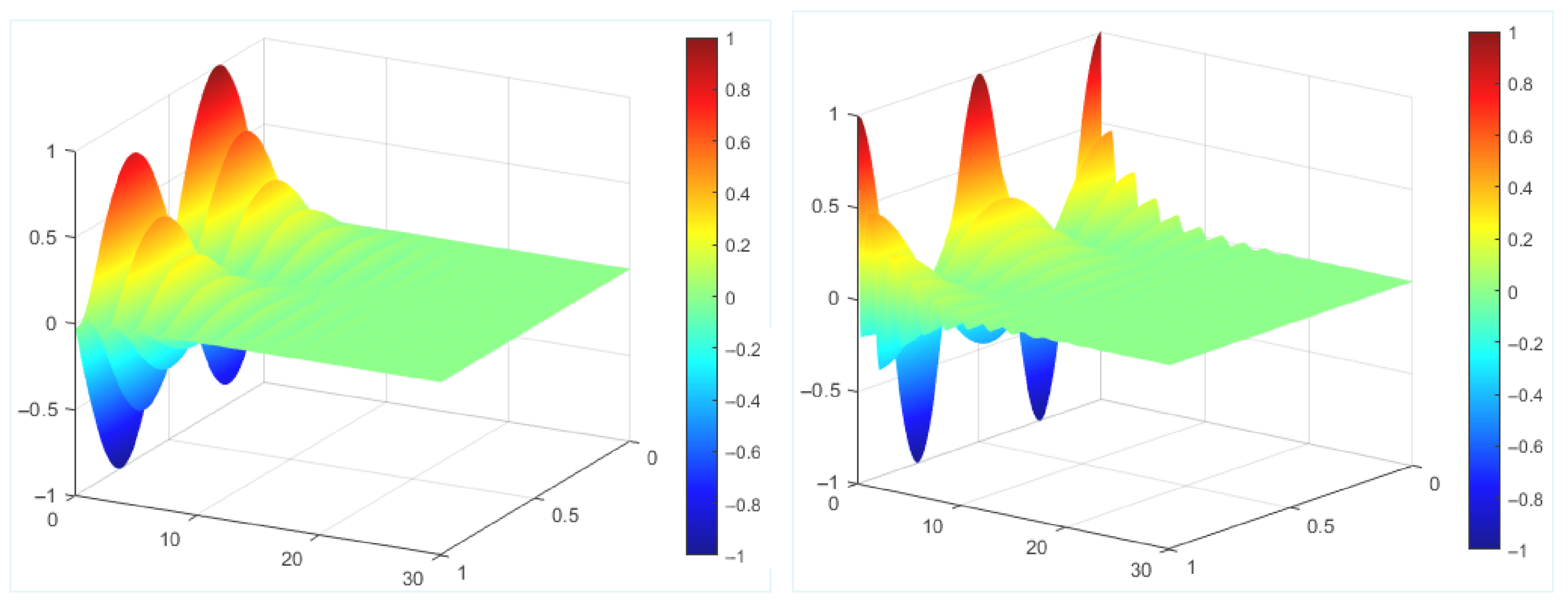
Figure 1 shows the evolution of the solution $\varphi$ (on the left) and $\psi$ (on the right) over time. Since the initial conditions given by (59) are sinusoidal functions in space, the numerical solutions plotted in (1) decay over time.

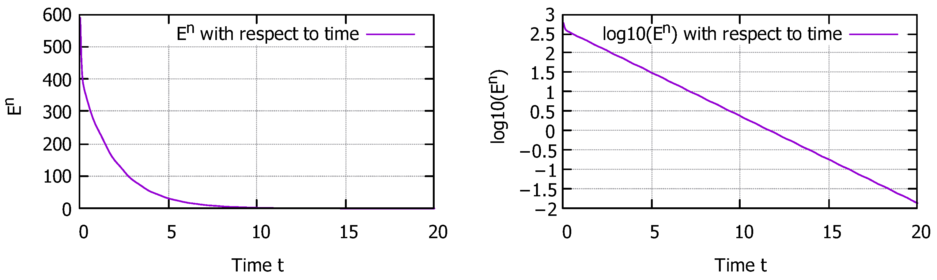
In the left part of Figure 2, we plot the energy $E^n$ with respect to time. To confirm the exponential decay, we plot in the right part of the same figure the function ${log}_{10}\left(E^n\right)$ over time. This figure confirms that the energy decays exponentially over time.

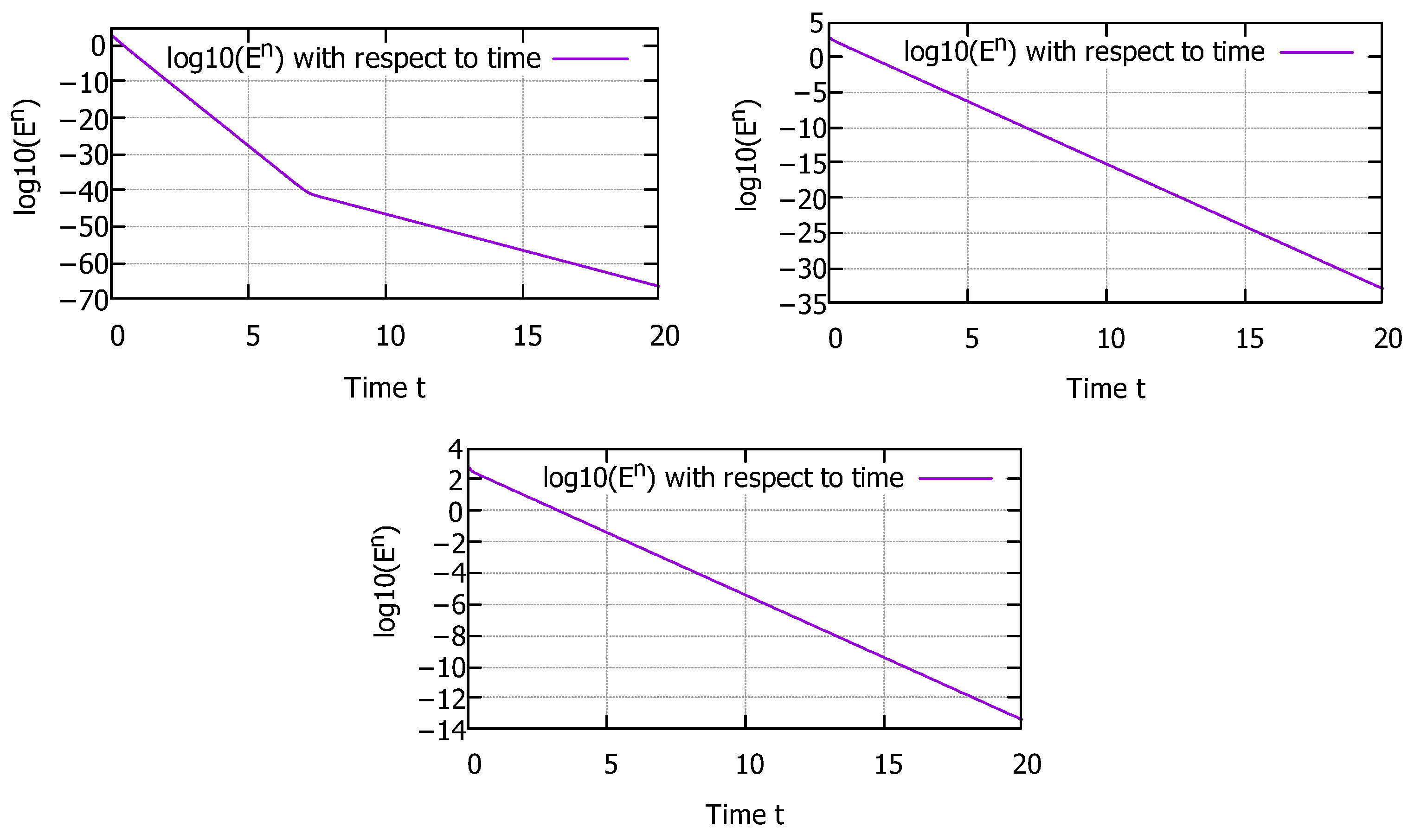
To illustrate how the exponential decay of energy depends on the parameter $\mu$, we perform simulations for $\mu =0,0.3$ and $0.7$ with $T=20$. Figure 3 show the energy on a logarithmic scale with respect to time and once again confirm the exponential decay of the energy $E^n$. The slopes of the corresponding lines are $-2.01$ for $\mu =0$, $-1.77$ for $\mu =0.3$ and $-0.43$ for $\mu =0.7$. We note that for $\mu =0$, we computed the corresponding slope for large times $t\ge 7$.

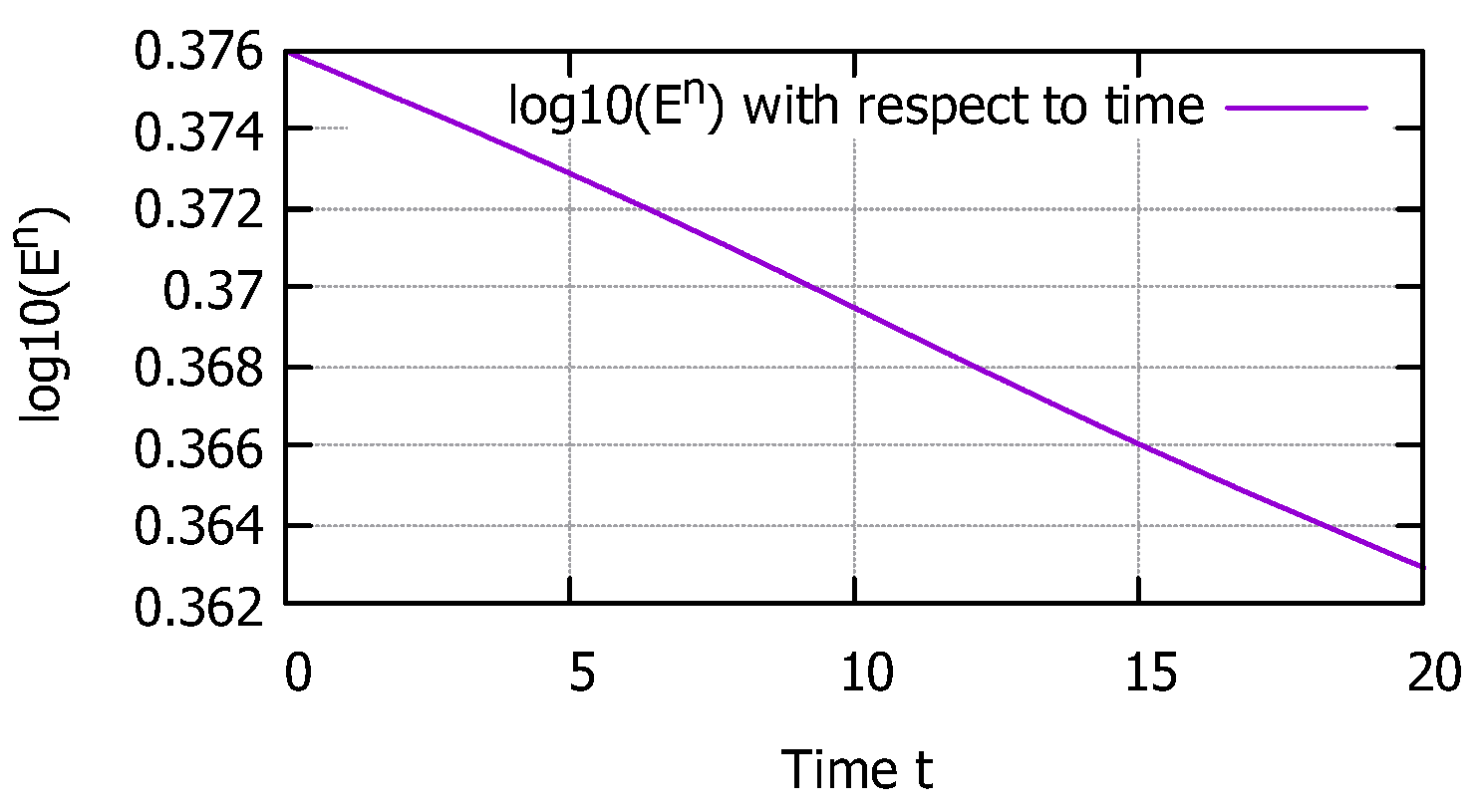
In the following, we perform a numerical simulation using physical parameters taken from reference [27], where ${\rho }_1=0.85$, ${\rho }_2=70.55 {10}^{-7}$, $k=65.365 {10}^{-4}$, $b=16.6 {10}^{-8}$, $\mu =0.5$ and $\beta =1.5$. Figure 4 shows the exponential decay of the energy over time.

6. Conclusions

In this work, we established the energy decay behavior of a nonlocal truncated Timoshenko–Ehrenfest system from a theoretical and numerical perspective. The well-posedness of the proposed model was first established using the Faedo–Galerkin method, ensuring the existence and uniqueness of solutions. By employing appropriate multiplier techniques, we derived energy stability results and proved the decay properties of the system.

Furthermore, a numerical scheme was developed to approximate the continuous model. Special attention was devoted to the exponential decay of the discrete energy, which reflects the stability properties observed at the continuous level. Numerical simulations were performed to illustrate the theoretical findings and to confirm the effectiveness of the proposed scheme.

Overall, this study provides a new viewpoint on the stability and energy decay of nonlocal truncated Timoshenko–Ehrenfest systems and offers a solid mathematical framework for their analysis. Future work may focus on extending these results to more general nonlocal models, nonlinear effects, or alternative discretization techniques, as well as exploring the influence of different material parameters on the decay behavior.

In this study, we have investigated the one-dimensional nonlocal Timoshenko–Ehrenfest beam model. Extending this analysis to multidimensional nonlocal systems will be an interesting direction for future research.

References

1. Eringen, A.C. Nonlocal polar elastic continua. Int. J. Eng. Sci. 1972, 10, 1–16. [Google Scholar] [CrossRef] [Scilit]
2. Eringen, A.C. On differential equations of nonlocal elasticity and solutions of screw dislocation and surface waves. J. Appl. Phys. 1983, 54, 4703–4710. [Google Scholar] [CrossRef] [Scilit]
3. Reddy, J.N. Nonlocal theories for bending, buckling and vibration of beams. Int. J. Eng. Sci. 2007, 45, 288–307. [Google Scholar] [CrossRef] [Scilit]
4. Timoshenko, S.P. On the correction for shear of the differential equation for transverse vibrations of prismatic bars. Philos. Mag. 1921, 41, 744–746. [Google Scholar] [CrossRef] [Scilit]
5. Soufyane, A. Stabilisation de la poutre de Timoshenko. C. R. Acad. Sci. Paris Ser. I Math. 1999, 328, 731–734. [Google Scholar] [CrossRef] [Scilit]
6. Malacarne, A.; Munoz Rivera, J.E. Lack of exponential stability to Timoshenko system with viscoelastic Kelvin–Voigt type. Z. Angew. Math. Phys. 2016, 67, 67. [Google Scholar] [CrossRef] [Scilit]
7. Almeida Junior, D.S.; Ramos, A.J.A. On the nature of dissipative Timoshenko systems at the light of the second spectrum. Z. Angew. Math. Phys. 2017, 68, 145. [Google Scholar] [CrossRef] [Scilit]
8. Elishakoff, I. An equation both more consistent and simpler than the Bresse–Timoshenko equation. In Advances in Mathematical Modelling and Experimental Methods for Materials and Structures; Springer: Dordrecht, The Netherlands, 2009; pp. 249–254. [Google Scholar] [CrossRef] [Scilit]
9. Zougheib, H.; El Arwadi, T.; Madureira, R.L.R.; Rincon, M.A. Do equal speed condition and exponential stability relate for the truncated thermoelastic Timoshenko system under Green–Naghdi law? J. Therm. Stresses 2023, 46, 673–705. [Google Scholar] [CrossRef] [Scilit]
10. Messaoudi, S.A.; Keddi, A.; Alahyane, M. On a truncated thermoelastic Timoshenko system with a dual-phase lag model. Math. Methods Appl. Sci. 2025, 48, 6691–6703. [Google Scholar] [CrossRef] [Scilit]
11. Ramos, A.J.A.; Almeida, D.S.; Miranda, L.G.R. An inverse inequality for a Bresse–Timoshenko system without second spectrum of frequency. Arch. Math. 2020, 114, 709–719. [Google Scholar] [CrossRef] [Scilit]
12. Almeida, D.S.; Ramos, A.J.A.; Santos, M.L.; Miranda, L.G.R. Asymptotic behavior of weakly dissipative Bresse–Timoshenko systems under the influence of the second spectrum of frequency. Z. Angew. Math. Mech. 2018, 98, 1320–1333. [Google Scholar] [CrossRef] [Scilit]
13. Almeida, D.S.; Elishakoff, I.; Ramos, A.J.A.; Miranda, L.G.R. The hypothesis of equal wave speeds for stabilization of the Bresse–Timoshenko system is not necessary anymore: The time-delay cases. IMA J. Appl. Math. 2019, 84, 763–796. [Google Scholar] [CrossRef] [Scilit]
14. Almeida, D.S.; Ramos, A.J.A.; Soufyane, A.; Cardoso, M.L.; Santos, M.L. Issues related to the second spectrum, Ostrogradsky’s energy, and the stabilization of Timoshenko–Ehrenfest-type systems. Acta Mech. 2020, 231, 3565–3581. [Google Scholar] [CrossRef] [Scilit]
15. Zougheib, H.; El Arwadi, T.; Bouraoui, H.A.; Djebabla, A. Stabilization of Lord–Shulman porous thermoelastic system from second spectrum viewpoint. Afr. Mat. 2025, 6, 85. [Google Scholar] [CrossRef] [Scilit]
16. Andrews, K.T.; Fernandez, J.R.; Shillor, M. Numerical analysis of dynamic thermoviscoelastic contact with damage of a rod. IMA J. Appl. Math. 2005, 70, 768–795. [Google Scholar] [CrossRef] [Scilit]
17. Campo, M.; Fernandez, J.R.; Kuttler, K.L.; Shillor, M.; Viano, J.M. Numerical analysis and simulations of a dynamic frictionless contact problem with damage. Comput. Methods Appl. Mech. Eng. 2006, 196, 476–488. [Google Scholar] [CrossRef] [Scilit]
18. Bochicchio, I.; Campo, M.; Fernandez, J.R.; Naso, M.G. Analysis of a thermoelastic Timoshenko beam model. Acta Mech. 2020, 231, 4111–4127. [Google Scholar] [CrossRef] [Scilit]
19. Aouadi, M.; Campo, M.; Copetti, M.I.M.; Fernandez, J.R. Existence, stability and numerical results for a Timoshenko beam with thermodiffusion effects. Z. Angew. Math. Phys. 2019, 70, 117. [Google Scholar] [CrossRef] [Scilit]
20. Copetti, M.I.M.; Fernandez, J.R. A dynamic contact problem involving a Timoshenko beam model. Appl. Numer. Math. 2013, 63, 117–128. [Google Scholar] [CrossRef] [Scilit]
21. Smith, R.W.M. Graphical representation of Timoshenko beam modes for clamped–clamped boundary conditions at high frequency: Beyond transverse deflection. Wave Motion 2008, 45, 785–794. [Google Scholar] [CrossRef] [Scilit]
22. Sayah, T.; El Arwadi, T. Exponential decay of the discrete energy for the wave–wave coupled system. Math. Mech. Solids 2025, 1–17. [Google Scholar] [CrossRef] [Scilit]
23. Zougheib, H.; El Arwadi, T.; Madureira, R.L.R.; Rincon, M.A.; Sayah, T. Exponential stability of a fully discrete energy associated to a thermoviscoelastic Timoshenko system. J. Therm. Stresses 2025, 1–16. [Google Scholar] [CrossRef] [Scilit]
24. De Rosa, M.A.; Lippiello, M.; Onorato, A.; Elishakoff, I. Free Vibration of Single-Walled Carbon Nanotubes Using Nonlocal Truncated Timoshenko-Ehrenfest Beam Theory. Appl. Mech. 2023, 4, 699–714. [Google Scholar] [CrossRef] [Scilit]
25. Lions, J.L. Quelques MeTHODES de ReSolution des PROBLeMES aux Limites Non Lineaires; Dunod Gauthier-Villars: Paris, France, 1969. [Google Scholar]
26. Hecht, F. New development in FreeFem++. J. Numer. Math. 2012, 20, 251–266. [Google Scholar] [CrossRef] [Scilit]
27. Kawano, A.; Brion, T.; Ichchou, M.; Zine, A. Uniqueness results for the Timoshenko beam model and identification of forces. Math. Eng. 2025, 7, 464–480. [Google Scholar] [CrossRef] [Scilit]
Figure 1. The evolution of the solutions ( ϕ on the left and ψ on the right) during time ( μ = 1 ).
Mathematics 14 01132 g001
Figure 2. The energy E n with respect to time: E n on the left and l o g 10 ( E n ) on the right ( μ = 1 ).
Mathematics 14 01132 g002
Figure 3. l o g 10 ( E n ) with respect to time: μ = 0 on the up-left, μ = 0.3 on the up-right and μ = 0.7 on down.
Mathematics 14 01132 g003
Figure 4. l o g 10 ( E n ) with respect to time t: ρ 1 = 0.85 , ρ 2 = 70.55 10 7 , k = 65.365 10 4 , b = 16.6 10 8 , μ = 0.5 and β = 1.5 .
Mathematics 14 01132 g004
Disclaimer/Publisher’s Note: The statements, opinions and data contained in all publications are solely those of the individual author(s) and contributor(s) and not of MDPI and/or the editor(s). MDPI and/or the editor(s) disclaim responsibility for any injury to people or property resulting from any ideas, methods, instructions or products referred to in the content.