Hybrid NN–ODE Modeling of Fossil Fuel Competition

Abstract

Europe’s fossil-based electricity mix has shifted rapidly in recent years, raising a practical question: can we model competitive substitution among fuels with a framework that is both predictive and interpretable? We address this by combining a compact neural network (NN) with a three-dimensional Lotka–Volterra (LV) system to study monthly EU coal, natural gas, and oil-fired generation shares from the second semester of 2017 to 2023. After converting the series to row-wise shares that sum to one, we use the first $70\%$ of the sample to learn smooth trajectories and data-driven derivatives with the NN and then estimate the LV interaction coefficients through a constrained nonlinear fit. We advance the calibrated LV system over the final $30\%$ holdout with a fourth-order Runge–Kutta (RK4) scheme and evaluate forecasts using the RMSE and MAE for each fuel share series. For comparison, we report the results against both a neural network-only forecasting baseline and a classical ARIMA benchmark, both trained on the same $70\%$ window and evaluated on the same $30\%$ holdout. The hybrid NN–LV model achieves competitive forecast errors while yielding interpretable interaction patterns consistent with substitution pressures (for example, negative cross-effects between coal and gas). Finally, we run counterfactual shock experiments to illustrate how a change in one fuel’s share propagates through the mix under the learned LV dynamics, highlighting the usefulness of embedding a simple mechanistic structure within a data-driven estimator.

1. Introduction

European electricity systems have been reorganized substantially over the past decade as fuel choices respond to carbon constraints, relative prices, and security-of-supply considerations. Within this setting, the composition of fossil-based generation is naturally viewed as a competitive system: increases in one component’s share compress the feasible space of the others at a given horizon. This paper models that competition among coal, natural gas, and oil-fired generation shares in the European Union using a compact framework designed to be interpretable, data-efficient, and consistent with share dynamics [1,2]. We treat the monthly mix as a closed three-component system and adopt a Lotka–Volterra (LV) specification in which self- and cross-effects encode how each component tends to grow or contract in the presence of the others [3].

When the variables of interest are shares, the modeling problem is intrinsically constrained: each observation lies on the unit simplex, and the three components sum to one at each time step. In such settings, parsimonious interaction models are preferable to unconstrained black-box architectures, because they encode structural restrictions that can be interrogated and stress-tested. The LV system is a canonical representation of interacting populations and technologies; the instantaneous growth of each component scales with its level and with the presence of others through parameters that capture self-reinforcement (diagonal) and competition or complementarity (off-diagonal) [3]. Interpreted in an energy mix context, negative cross-effects indicate substitution pressure—for instance, higher gas share, making it harder for coal to expand—while a positive self-effect captures short-run persistence. Related work in competitive market shares further supports the usefulness of such low-dimensional interaction systems for rivalry and substitution [4].

Methodologically, we use a hybrid design: a small feed-forward neural network (NN) is trained on the earliest portion of the sample to produce smooth trajectories and data-driven derivative estimates. These derivatives are then used to estimate the Lotka–Volterra (LV) interaction coefficients. The fitted system is subsequently advanced over the holdout window using a classical fourth-order Runge–Kutta (RK4) integrator [5]. This NN → LV → RK4 pipeline preserves interpretability through the LV coefficients while leveraging the NN’s approximation ability for mildly nonlinear dynamics and remains intentionally compact to ease estimation, diagnostics, and reproducibility.

Across Europe, coal’s share of electricity generation has declined markedly since 2010. It saw a brief uptick in 2021–2022 before resuming its downward trend. Gas has often played a swing role, while oil-fired generation has become small but remains nonzero [6,7]. From an economic perspective, these shifts are manifestations of interfuel substitution, a long-studied topic in power generation using systems such as translog cost or share equations to quantify elasticities among coal, gas, and oil [8,9,10,11]. Carbon pricing via the EU Emissions Trading System (ETS) and relative commodity prices can trigger coal-to-gas switching when spreads are favorable [12,13]. Sectoral reviews document the broader backdrop of changing fuel contributions and price dynamics in recent years [14]. In this environment, LV provides a compact way to summarize competitive pressures directly in shares, producing coefficients that can be interpreted alongside observed price and policy regimes.

Because the data are proportions, we normalize row-wise so that the shares sum to one each month. This avoids offsets or centering that could violate the Lotka–Volterra model’s multiplicative structure and lead to negative state values [15]. Identification proceeds in two layers. First, the NN provides smoothed trajectories and estimated derivatives for each component on the training slice. Second, we estimate the LV interaction matrix by least squares to match NN-implied derivatives with LV-implied right-hand sides, with mild regularization for stability. The fitted LV parameters offer a concise summary of the system’s interaction structure, while the RK4 solver propagates the system over the test slice [16]. We monitor adherence to the simplex (sum of shares near one; no negative values) during estimation and forecasting and report any deviations as numerical diagnostics.

For evaluation, we use a strictly chronological holdout: train on the earliest portion of the sample and forecast the final segment. In line with standard time-series testing practice, we report the root-mean-square error (RMSE) and mean absolute error (MAE) on the held-out months [17,18,19]. As a sole comparator, we include a direct neural network forecasting baseline that predicts the share trajectories without imposing an explicit dynamical law. This isolates the value added by coupling the network with the Lotka–Volterra structure and RK4 integration. In addition to the chronological split, we employ a moving-block bootstrap within NN training only to stabilize derivative estimation and to select network weights using an out-of-bag (OOB) loss. Final forecasting and all reported metrics are based on the chronological holdout window, not on bootstrap-based validation.

The idea for this work grew out of a practical modeling gap we kept running into: purely data-driven forecasts tracked short-term movements, but they offered little structure for interpreting substitution among coal, gas and oil. We therefore combined a deep neural network with a Lotka–Volterra system and used the resulting model to forecast and to run counterfactual shock experiments. First, we curate and preprocess a monthly EU dataset for coal, gas and oil-fired generation and cast it as a closed three-component system aligned with a Lotka–Volterra interaction model. Second, we estimate a $3\times 3$ LV system using NN-assisted parameter identification and advance the fitted dynamics with a fourth-order Runge–Kutta scheme in MATLAB, combining forecasting performance with structural interpretability. Finally, we benchmark the hybrid NN-LV framework against both a neural network-only forecast baseline and a classical ARIMA benchmark, and we show that, on the reported holdout window, the hybrid model achieves lower forecast errors while retaining interpretable interaction coefficients.

The remainder of this paper is organized as follows: Section 2 reviews related work on competition models (including Lotka–Volterra), compositional shares, and hybrid neural/ODE estimation. Section 3 describes the data and preprocessing, including the construction of monthly EU coal–gas–oil shares. Section 4 presents the modeling framework (neural network estimator, LV specification, Runge–Kutta integration). It also details the validation protocol and the NN baseline (chronological holdout, RMSE and MAE) and clarifies the use of moving-block bootstrap within NN training only. Section 5 reports the numerical results. Section 6 presents a discussion about the basic findings and prospects for future research. Section 7 consists of conclusions.

2. Related Work

A large body of work models competition and substitution in markets using compact interaction systems, with Lotka–Volterra-type equations as a common starting point. In energy and electricity contexts, LV has been used to describe market penetration paths and share interactions among technologies, including renewable versus conventional generation and other competing carriers, precisely because it turns “who gains when others grow” into a small set of interpretable coefficients [20,21]. Recent applications revisit LV for clean energy diffusion and competitive dynamics under contemporary policy and price regimes [22], while related studies apply LV-style systems to energy consumption and emissions in national settings [23]. There is also a parallel “gray LV” line aimed at forecasting when data are short and noise is high, which still relies on the idea that a few interaction terms can summarize substitutability or cooperation over medium horizons [24,25]. Outside energy, LV has been used to capture market share rivalry in technology and telecom markets, supporting the claim that a low-dimensional interaction matrix can be both tractable and informative for competitive settings [4].

Because the targets here are shares, the methodological backdrop is compositional data analysis. Shares live on the unit simplex and carry primarily relative information, so modeling choices should avoid spurious correlation and respect the geometry of the data [15]. Foundational and recent reviews discuss when to transform with logratio mappings, when to work directly in constrained space, and how to design diagnostics that check adherence to the simplex in estimation and forecasting [26,27,28,29]. In practice, two principles recur: treat observations as rows that sum to one and ensure that any simulation step (here, ODE integration) maintains or closely respects that constraint. These ideas justify the use of row-wise shares and the attention to share sum deviation in evaluation.

On the learning side, neural ordinary differential equations offer a way to learn vector fields from data and then propagate them with standard solvers [30]. In power system applications, neural ODEs and related hybrid schemes have been explored for demand and building thermal forecasting, typically with small, physics-informed structures that balance flexibility with interpretability [31,32,33]. A complementary thread, physics-informed neural networks, makes the same case from a different angle: blend data fitting with mechanistic constraints to improve generalization and credibility [34]. The present work follows the compact end of this spectrum: A small neural network estimates smooth trajectories and derivatives, an LV system provides the structural backbone, and a classical solver advances the state. This architecture is designed to keep parameters interpretable while still capturing the mild nonlinearities present in monthly fuel shares.

Finally, benchmarking against transparent time-series references remains standard in energy forecasting, especially when the goal is to justify a new modeling pipeline rather than to “win” with a black-box predictor. In our case, we use a strict chronological holdout and report the RMSE and MAE, which is consistent with common practice and keeps the comparison reproducible and fair across methods trained on the same information set [17,18]. In addition to the like-for-like neural baseline, we now also include a classical ARIMA benchmark, selected from a set of low-order candidates according to the lowest mean holdout RMSE across the three series. This expanded benchmark design still keeps the comparison focused: the NN baseline isolates what the LV structure and RK4 evolution add beyond a purely data-driven fit, while the ARIMA model provides a transparent statistical reference. Framing the related work in a dedicated section then makes the contribution clearer: we combine interpretable interaction dynamics from competition models, the practical constraints of compositional shares, and a compact neural learning component for derivative estimation and parameter identification, and we evaluate the resulting hybrid model against both neural-only and ARIMA forecasts on monthly EU coal–gas–oil shares.

3. Data and Preprocessing

3.1. Sources, Scope, and Time Window

We compile monthly net electricity generation by fuel for the European Union from Eurostat’s official series Net electricity generation by type of fuel (dataset code nrg_cb_pem) and use it to construct fossil fuel shares for coal, natural gas, and oil. (Eurostat nrg_cb_pem, monthly frequency; see the dataset landing page and DOI metadata for structure and update policy.) The full dataset is provided in the Supplementary Materials (File S1). Unless otherwise noted, the geographic aggregate is EU27; for months where the standard EU27 aggregate is not published in the chosen window, we fall back to the EU28 aggregate and re-map to ensure a consistent EU27 coverage [35,36]. 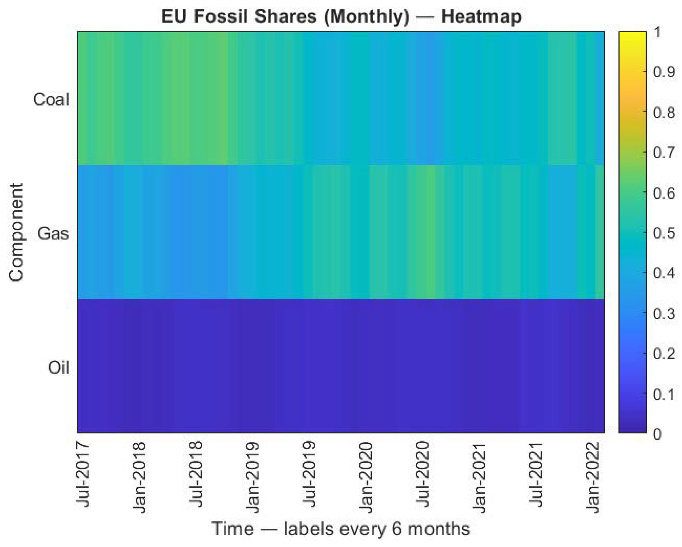As we see in Figure 1 the analysis window used in the empirical section is stated here explicitly: from July 2017 to December 2023, inclusive (78 monthly observations).

We use Eurostat as the primary source to avoid mixing definitions across providers. For cross-checks on broad trends (not used directly in estimation), we consult Ember’s European Electricity Review and its data methodology notes, which document monthly compilation practices and known issues around technology/fuel classifications and backfills [7,37].

3.2. Units and Transformations

Eurostat reports monthly net generation in GWh by fuel category. We convert each month’s coal, gas, and oil values into row-wise shares so they sum to one by construction:

$$s_{j,t}={\displaystyle \frac{y_{j,t}}{y_{\mathrm{coal},t}+y_{\mathrm{gas},t}+y_{\mathrm{oil},t}}},j\in \left\{\mathrm{coal},\mathrm{gas},\mathrm{oil}\right\}.$$

Working directly in share space avoids negative states and respects the multiplicative structure assumed by Lotka–Volterra interactions for compositional data [15]. No seasonal adjustment is applied to the levels prior to forming shares, and also the seasonality in fossil generation is largely absorbed by normalization and the LV dynamics over shares. For numerical conditioning inside the neural module only, inputs on the time axis are standardized to zero mean and unit variance. Also all targets, parameter estimation, and evaluation remain in the original share space (i.e., bounded in $[0,1]$ and summing to one).

3.3. Completeness and Harmonization

The monthly panel is complete over the stated window: there are no missing months. Where Eurostat’s monthly taxonomy for fossil fuels differs slightly across revisions (e.g., coal and manufactured gases within SIEC groupings), we map to a stable triplet (coal, natural gas, oil and petroleum products) following Eurostat’s SIEC documentation, and any reclassifications are applied consistently across the window to preserve comparability [35,36].

3.4. Preprocessing Steps

• Extraction and filtering: We download monthly EU aggregates for coal, natural gas, and oil from nrg_cb_pem; retain EU27, with EU28 used only as a fallback where EU27 is not available in early months, then harmonize to EU27.
• Share construction: We convert GWh to monthly shares as above, and we also check for zeros or tiny denominators before division (none occur over the window).
• Outlier scan: Visual screening flagged a few one-off reporting spikes. None require intervention. We avoid aggressive filters that could distort the competitive share dynamics.
• NN internals: We standardize time inputs, not the shares. No de-meaning or centering of shares is performed to keep the LV multiplicative form intact.
• Simplex checks: During training and identification, we monitor (but do not enforce) the simplex: we report the mean and maximum $\left|{\sum }_j{s}_{j,t}-1\right|$ and flag any $s_{j,t}\notin [0,1]$. During forecasting, we likewise monitor and report these diagnostics on the RK4 trajectories. In our implementation, the training window diagnostics were $\mathrm{mean}|\mathrm{sum}-1|=9.4304\times {10}^{-4}$ and $\max |\mathrm{sum}-1|=1.9631\times {10}^{-3}$, with 0 months containing any negative component and 0 months containing any component exceeding 1 [17].

3.5. Coverage and Quality Diagnostics

To document reproducibility and data quality, we provide a concise diagnostic panel:

3.5.1. Coverage

First month: 2017–07; last month: 2023–12; total observations: 78. All months present with no gaps.

3.5.2. Descriptive Statistics (Shares)

Over the window, coal’s median share is low and declining. Gas exhibits higher variability and frequently plays a swing role. Oil remains small but nonzero. We report the per-series mean, standard deviation, and 5th–95th percentiles, plus the mean and max of $|{\sum }_j{s}_{j,t}-1|$ (expected near numerical zero).

3.5.3. Seasonality

Monthly seasonality in fossil shares is muted relative to levels (as intended by the share construction), but weak intra-year patterns persist. We display (i) monthly boxplots of shares by calendar month and (ii) a simple seasonal subseries plot. Such visuals are standard in electricity forecasting to understand residual seasonality and guide baseline model choices [38].

3.5.4. Cross-Checks

Aggregate EU trends visually align with sectoral narratives documented in independent reviews (coal decline with a 2021–2022 uptick, gas as the margin fuel, oil small), providing a sanity check that the constructed shares track recognized dynamics [7].

These steps yield a clean, complete monthly EU panel of coal–gas–oil shares suitable for the NN–LV–RK4 pipeline while keeping preprocessing minimal and transparent in line with the best practices in energy forecasting.

4. Compact NN-ODE Pipeline for Share Dynamics and Forecasting

This section presents a simple pipeline for estimating interaction parameters in nonlinear ordinary differential equations (ODEs). We combine a small deep neural network (DNN) with a three-variable Lotka–Volterra (LV) system. The DNN is used to learn smooth share paths over time and to supply analytic time derivatives. We then estimate the LV coefficients by matching the LV right-hand sides to these derivatives with nonlinear least squares. Finally, we simulate the fitted LV model forward with a standard ODE solver and evaluate forecasting accuracy.

We apply the method to monthly European electricity shares for coal, natural gas, and oil. The goal is to keep the model compact, easy to reproduce, and interpretable in terms of “who competes with whom” among the three fuels.

4.1. Mathematical Setup and Interaction Model

Algorithm 1 summarizes the full workflow. Let $u_1,u_2,u_3$ denote the shares of coal, gas, and oil. We use a generalized three-component Lotka–Volterra system,

$$\begin{array}{ccc}\hfill {\displaystyle \frac{d{u}_1}{dt}}& =& u_1\left(p_1+p_2{u}_1+p_3{u}_2+p_4{u}_3\right),\hfill \\ \hfill {\displaystyle \frac{d{u}_2}{dt}}& =& u_2\left(p_5+p_6{u}_1+p_7{u}_2+p_8{u}_3\right),\hfill \\ \hfill {\displaystyle \frac{d{u}_3}{dt}}& =& u_3\left(p_9+p_{10}{u}_1+p_{11}{u}_2+p_{12}{u}_3\right).\hfill \end{array}$$

(1)

Algorithm 1 Training-to-estimation pipeline (DNN → LV parameters → RK4 simulation)

1: Input: EU monthly fossil-share data (Excel), time vector $t\_data={[0,1,\dots ,N-1]}^T$ 2: Read and preprocess $[\mathrm{Coal},\mathrm{Gas},\mathrm{Oil}]$ into $data$ 3: Chronological split: 70% training ($train\_data$, $train\_time$), 30% testing ($test\_data$, $test\_time$) 4: Define a DNN with three hidden layers (tanh) and linear output, initialize small random weights 5: Retain placeholders for the best weights and minimum out-of-bag (OOB) cost 6: for bootstrap replicate $b=1$ to 5 do 7:       Build moving-block bootstrap indices (block length $=5$) on the training slice 8:       Form resampled $train\_dat{a}^{\left(b\right)}$, $train\_tim{e}^{\left(b\right)}$ 9:       Fit the DNN on $train\_tim{e}^{\left(b\right)}$ to produce smooth shares $\widehat{U}\left(t\right)$ 10:     Obtain analytic derivatives $\dot{\widehat{U}}\left(t\right)$ by differentiating the network via the chain rule 11:     Compute OOB validation cost on left-out training points 12:     if current OOB cost < best so far then 13:           Save current weights as “best” 14:     end if 15: end for 16: With best weights, compute $\widehat{U}$ and ${\displaystyle \frac{d{\widehat{u}}_1}{dt}},{\displaystyle \frac{d{\widehat{u}}_2}{dt}},{\displaystyle \frac{d{\widehat{u}}_3}{dt}}$ on the training grid 17: Specify LV: ${\dot{u}}_i=u_i(p_{i1}+p_{i2}{u}_1+p_{i3}{u}_2+p_{i4}{u}_3)$ for $i=1,2,3$ 18: Estimate $p_1,\dots ,p_{12}$ by nonlinear least squares on the training grid 19: Report parameter estimates and standard errors 20: Integrate the fitted LV on the test grid using the classical fourth-order Runge–Kutta scheme

4.2. Parameter Estimation via Derivative Matching

The DNN is trained on the training window to approximate monthly share paths $t\mapsto \widehat{\mathbf{u}}\left(t\right)$. Because the network is a smooth function of time, we can compute ${\displaystyle \frac{d\widehat{\mathbf{u}}}{dt}}$ analytically using the chain rule. We then estimate $p_1,\dots ,p_{12}$ by matching LV slopes to these DNN-based slopes.

Define the stacked residual

$$\begin{array}{ccc}\hfill r\left(p\right)& =& \left[\begin{array}{c}{\displaystyle \frac{d{\widehat{u}}_1}{dt}-{\widehat{u}}_1\left(p_1+p_2{\widehat{u}}_1+p_3{\widehat{u}}_2+p_4{\widehat{u}}_3\right)}\\ {\displaystyle \frac{d{\widehat{u}}_2}{dt}-{\widehat{u}}_2\left(p_5+p_6{\widehat{u}}_1+p_7{\widehat{u}}_2+p_8{\widehat{u}}_3\right)}\\ {\displaystyle \frac{d{\widehat{u}}_3}{dt}-{\widehat{u}}_3\left(p_9+p_{10}{\widehat{u}}_1+p_{11}{\widehat{u}}_2+p_{12}{\widehat{u}}_3\right)}\end{array}\right],\hfill \end{array}$$

(2)

and estimate p by

$$\underset{p}{min}{∥r\left(p\right)∥}_2^2.$$

(3)

This produces a small, interpretable set of interaction coefficients that can be used directly for simulation and forecasting.

4.3. Neural Module for Monthly Shares

4.3.1. Architecture

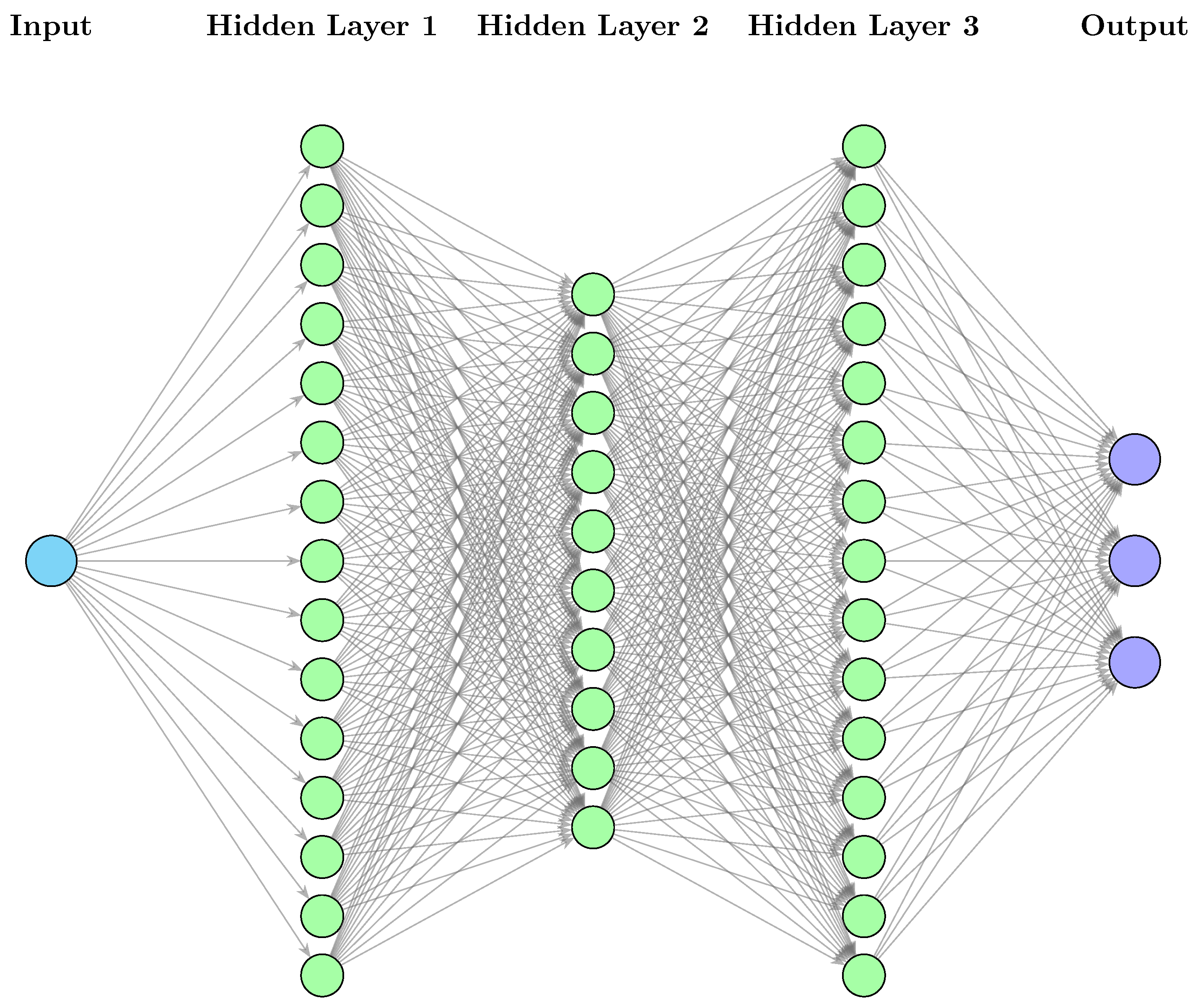
As we see in Figure 2 we use a three-hidden-layer DNN (15, 10 and 15 units) with tanh activations and a linear three-node output (coal, gas, oil). We use a tanh activation in the hidden layers because it yields smooth bounded hidden representations and analytically differentiable mappings, which is useful here since the NN is employed not only for fitting trajectories but also for extracting implied time derivatives. See Algorithm 2 for the full architecture search and training procedure. The single input is time t. Weights are initialized near zero, and biases are set small to keep activations responsive early in training.

Algorithm 2 Neural architecture search with bootstrap validation

1: Input: EU fossil shares, hidden sizes $h_1,h_2,h_3\in \{5,10,15\}$, learning rates $\{0.00001,0.00003\}$, epochs $\{100,200\}$ 2: for each $(h_1,h_2,h_3)$, learning rate, epoch count do 3:       for bootstrap replicate $b=1$ to 5 do 4:             Train DNN on a moving-block bootstrap sample of the training data 5:             Compute OOB validation cost on left-out training months 6:             Keep weights for the replicate with the smallest OOB cost 7:       end for 8:       Estimate LV via least squares using NN output on the training window, simulate with RK4 on the training window, compute RMSE for Coal, Gas, Oil 9:       Store configuration and RMSE 10: end for 11: Rank configurations by training-window mean RMSE (RK4 simulation) and retain the top 5

4.3.2. What the DNN Provides

The network serves two roles. (i) It produces smooth trajectories ${\widehat{u}}_1\left(t\right),{\widehat{u}}_2\left(t\right),{\widehat{u}}_3\left(t\right)$. (ii) It provides analytic derivatives ${\displaystyle \frac{d{\widehat{u}}_i}{dt}}$, avoiding noisy finite differences on short series.

4.3.3. Forward Propagation Recap

Given input $t^{\left(m\right)}$, layer pre-activations and activations satisfy

$${\mathbf{c}}^{\ell }=W^{\ell }{\mathbf{r}}^{\ell -1}+{\mathbf{b}}^{\ell },{\mathbf{r}}^{\ell }={\sigma }^{\ell }\left({\mathbf{c}}^{\ell }\right),$$

(4)

with ${\sigma }^{\ell }=tanh$ on hidden layers and identity on the output. Stacking all inputs $T=[t_1,\dots ,t_N]$ gives $C^{\ell }=W^{\ell }{A}^{\ell -1}+{\mathbf{b}}^{\ell }$ and $A^{\ell }={\sigma }^{\ell }\left(C^{\ell }\right)$ (with $A^0=T$), yielding final output $A^L=N(T,W,\mathbf{b})$. We use the chain rule through (4) to compute ${\displaystyle \frac{d\widehat{\mathbf{u}}}{dt}}$ exactly.

4.4. Uncertainty Analysis and Final Calibrated Lotka–Volterra System

After estimating p by nonlinear least squares, we add a basic uncertainty check. We approximate the local parameter covariance using the Jacobian of the residual function and report standard errors and 95% confidence intervals. Coefficients with narrow intervals are more stable in the data, while wide intervals should be treated with more caution. These intervals are based on a local Jacobian approximation of the second-stage least-squares problem and should be interpreted as conditional on the NN-implied trajectories and derivatives used for identification. They do not propagate uncertainty from neural network training and bootstrap weight selection through to the LV parameters.

In this setting, the reported intervals are the most informative for distinguishing relatively stable interaction patterns from weaker coefficients that remain only loosely identified by the available sample. For completeness, we also write the calibrated three-component system using the estimated coefficients in

Table 1. Parameter estimates with uncertainty quantification (standard error and 95% confidence interval).

Parameter	Estimate	Std (Uncertainty)	95% CI Range	Uncertainty Level
$p_1$	−0.0806	0.0631	[−0.2043, 0.0430]	Medium
$p_2$	0.0784	0.0638	[−0.0466, 0.2034]	Medium
$p_3$	−0.0153	0.0676	[−0.1478, 0.1171]	Medium
$p_4$	0.8836	0.0382	[0.8089, 0.9584]	Low
$p_5$	0.4078	0.0899	[0.2316, 0.5841]	Medium
$p_6$	−0.3911	0.0909	[−0.5692, −0.2130]	Medium
$p_7$	−0.2985	0.0955	[−0.4856, −0.1114]	Medium
$p_8$	−1.5054	0.0560	[−1.6152, −1.3956]	Low
$p_9$	−0.5773	0.8658	[−2.2742, 1.1197]	High
$p_{10}$	0.5976	0.8749	[−1.1173, 2.3125]	High
$p_{11}$	0.8300	0.9208	[−0.9747, 2.6348]	High
$p_{12}$	−2.0000	0.5322	[−3.0432, −0.9568]	High

Note: Intervals are conditional on NN-implied derivatives (local least-squares approximation).

. Here $x\left(t\right),y\left(t\right),z\left(t\right)$ denote coal, gas, and oil shares.

$$\begin{array}{ccc}\hfill {\displaystyle \frac{dx}{dt}}& =& x\left(-0.0806+0.0784x-0.0153y+0.8836z\right),\hfill \\ \hfill {\displaystyle \frac{dy}{dt}}& =& y\left(0.4078-0.3911x-0.2985y-1.5054z\right),\hfill \\ \hfill {\displaystyle \frac{dz}{dt}}& =& z\left(-0.5773+0.5976x+0.8300y-2.0000z\right).\hfill \end{array}$$

(5)

4.5. Numerical Propagation with RK4 and Simplex Handling

Several families of ODE solvers exist, including Runge–Kutta(–Nyström) and linear multistep methods (see [5,39,40,41,42,43]). We integrate the fitted LV system (1) using the classical fourth-order Runge–Kutta method [5]:

$${\displaystyle \frac{dy}{dt}}=f(t,y),y\left(t_0\right)=y_0.$$

(6)

The Runge–Kutta method approximates the solution to (6) through

$$\begin{array}{ccc}\hfill y_{n+1}& =& y_n+h\sum _{i=1}^s{b}_i{k}_i,\hfill \end{array}$$

(7)

$$\begin{array}{ccc}\hfill k_i& =& f\left(t_n+c_{i}h,y_n+h\sum _{j=1}^{i-1}{a}_{ij}{k}_j\right),\mathrm{for}i=1,2,\dots ,s,\hfill \end{array}$$

where h is the step size, s is the number of stages, and $a_{ij},b_i,c_i$ define the scheme.

For RK4 with four stages [5],

$$\begin{array}{ccc}\hfill k_1& =& f\left(t_n,y_n\right),\hfill \end{array}$$

$$\begin{array}{ccc}\hfill k_2& =& f\left(t_n+c_{2}h,y_n+\left(a_{21}{k}_1\right)h\right),\hfill \end{array}$$

$$\begin{array}{ccc}\hfill k_3& =& f\left(t_n+c_{3}h,y_n+\left(a_{31}{k}_1+a_{32}{k}_2\right)h\right),\hfill \end{array}$$

(8)

$$\begin{array}{ccc}\hfill k_4& =& f\left(t_n+c_{4}h,y_n+\left(a_{41}{k}_1+a_{42}{k}_2+a_{43}{k}_3\right)h\right),\hfill \end{array}$$

$$\begin{array}{ccc}\hfill y_{n+1}& =& y_n+h\left(b_1{k}_1+b_2{k}_2+b_3{k}_3+b_4{k}_4\right).\hfill \end{array}$$

(9)

The classical RK4 coefficients (Butcher tableau) are

$$\begin{array}{c}0\\ {\displaystyle \frac{1}{2}}& {\displaystyle \frac{1}{2}}\\ {\displaystyle \frac{1}{2}}& 0& {\displaystyle \frac{1}{2}}\\ 1& 0& 0& 1\\ & {\displaystyle \frac{1}{6}}& {\displaystyle \frac{1}{3}}& {\displaystyle \frac{1}{3}}& {\displaystyle \frac{1}{6}}\end{array}$$

The RK4 step size is set equal to one month so that numerical propagation is carried out on the same temporal grid as the observed data.

Compositional validity: Shares should be nonnegative and sum to one. During DNN fitting, we monitor ${\sum }_i{\widehat{u}}_i\left(t\right)$ as a basic check. During LV simulation with RK4, we do not impose a projection or renormalization step inside the integrator; instead we report diagnostics quantifying any drift from the simplex (mean and maximum absolute deviation of the share sum from one and counts of months where any simulated share falls outside $[0,1]$). These diagnostics make numerical validity transparent without altering the simulated dynamics.

4.6. Validation Protocol: Split, Bootstrap, and Model Selection

All reported results are based on a strict chronological split: the first 70% of months form the training window, and the last 30% form the holdout window. The DNN is trained only on the training window, and LV parameters are estimated using the same window. This separation between model construction and final evaluation follows standard internal validation principles for predictive modeling [44]. Forecasting then starts from the last observed state in training and integrates the fitted LV forward over the holdout window. The LV parameters are not re-estimated on the holdout period. All RMSE values used to rank candidate network configurations in the architecture search are computed on the training window only (in-sample RK4 simulation), and the holdout window is used only once for final reporting. The empirical results should therefore be interpreted as evidence from one strict chronological holdout exercise, not as a complete robustness assessment across multiple forecast origins.

To stabilize weight selection on a short time series, we use a moving-block bootstrap inside the training window only (block length $=5$), following the general bootstrap resampling principle [45]. The moving-block bootstrap uses a block length of five months as a compromise between preserving short-range temporal dependence and retaining a meaningful number of resampled blocks within a short training window. For each bootstrap replicate, we train the DNN and compute an out-of-bag (OOB) cost on the left-out training points. We keep the weights with the lowest OOB cost. This resampling step is used only for choosing network weights. It is not used to define the main test score, which always comes from the final 30% holdout.

From Algorithm 2, the search covers $3^3=27$ three-hidden-layer architectures (5–10–15 neurons per layer), for each learning rate and epoch choice.

This ranking is based solely on training window simulation error; the holdout window remains untouched until the final evaluation reported in a later section The hyperparameter grid was intentionally restricted to a small set of compact architectures, learning rates, and epoch counts. Given the short sample and the role of the NN as a smooth derivative estimator rather than a standalone high-capacity forecaster, the goal was to select a parsimonious and stable configuration rather than to exhaust the hyperparameter space.

Given

Table 2. Per-series RMSEs (coal, gas, oil) and mean RMSE (MRMSE) for candidate DNN configurations (hidden sizes restricted to multiples of five).

${\mathit{h}}_1$	${\mathit{h}}_2$	${\mathit{h}}_3$	Coal	Gas	Oil	MRMSE	OOB Cost
15	10	15	0.051257	0.056023	0.0059045	0.037728	0.0030304
5	10	10	0.054304	0.053522	0.0067756	0.038201	0.0024806
15	15	10	0.054565	0.053395	0.0076153	0.038525	0.0041206
5	5	15	0.055702	0.054851	0.0071888	0.039247	0.0025897
15	5	15	0.056129	0.054868	0.0069736	0.039324	0.0022749

, we select the configuration with the lowest mean RMSE. After selection, we estimate the LV coefficients on the training window and solve the system with RK4 over the holdout window.

4.7. Error Metrics and Simplex Diagnostics

Forecast accuracy is summarized using the root-mean-square error (RMSE) and mean absolute error (MAE). For an observed series $y_i\left(t\right)$ and prediction ${\widehat{y}}_i\left(t\right)$ over $t=1,\dots ,T_{\mathrm{test}}$ in the holdout window,

$${\mathrm{RMSE}}_i=\sqrt{{\displaystyle \frac{1}{T_{\mathrm{test}}}}\sum _{t=1}^{T_{\mathrm{test}}}{\left(y_i\left(t\right)-{\widehat{y}}_i\left(t\right)\right)}^2},$$

(10)

and

$${\mathrm{MAE}}_i={\displaystyle \frac{1}{T_{\mathrm{test}}}}\sum _{t=1}^{T_{\mathrm{test}}}\left|y_i\left(t\right)-{\widehat{y}}_i\left(t\right)\right|.$$

(11)

We report per-series scores and simple averages across coal, gas, and oil [17,18,19].

Because the targets are shares, we also report two basic diagnostics: (i) the deviation of the share sum from one,

$$\left|{\widehat{u}}_{\mathrm{coal}}\left(t\right)+{\widehat{u}}_{\mathrm{gas}}\left(t\right)+{\widehat{u}}_{\mathrm{oil}}\left(t\right)-1\right|,$$

and (ii) the count of any months where the raw solver step would produce a negative share or a share above one (as produced by the solver).

4.8. Benchmark Model

Neural network forecast baseline (NN-only): As a basic baseline, we use the same DNN trained on the same 70% training window, but we treat it as a direct forecaster of the share trajectories. The NN-only baseline does not compute derivatives, does not estimate LV coefficients and does not integrate an ODE. Any improvement in NN–LV–RK4 over NN-only can therefore be attributed to the added LV structure and the forward simulation step, rather than to a larger network. As an additional classical benchmark, we estimated univariate ARIMA models separately for the coal, gas, and oil share series on the same chronological training window. We tested several low-order ARIMA specifications and retained ARIMA(2, 0, 2), which delivered the best forecasting performance among the ARIMA candidates considered. The resulting ARIMA forecasts were then evaluated on the same holdout window as the NN-only and NN-LV-RK4 models.

4.9. Computational Footprint and Practicality

The pipeline is designed to be lightweight.

• The DNN has a single scalar input (time), three small hidden layers (widths from {5, 10, 15}), and three outputs. Training with Adam for a few hundred epochs on monthly data is fast in MATLAB (R2024a) on a desktop equipped with an NVIDIA GeForce MX450 (16 GB) and an Intel i7 3.3GHz CPU.
• The LV model has only 12 parameters, estimated by nonlinear least squares (e.g., lsqnonlin) using analytic derivatives from the trained network. The small parameter vector typically converges quickly.
• Forecasting is done with RK4 at monthly resolution, which is computationally trivial.

Compared with heavier deep learning models often used in energy forecasting [46,47], this approach keeps computation modest while still providing an interpretable interaction structure. The validation protocol is built to answer three practical questions: (i) does NN–LV–RK4 forecast the holdout period better than ARIMA and NN-only trained on the same window, (ii) are the forecasts numerically sensible for shares (nonnegative and summing close to one), and (iii) can the model be trained and re-estimated quickly with a small, readable set of parameters?

5. Numerical Results

This section reports the out-of-sample performance of the proposed NN-ODE framework on monthly EU fossil fuel shares (coal, gas, oil) under a chronological 70/30 split. We compare the hybrid approach against an ARIMA model and a purely neural network forecasting baseline trained on the same training window. We then use the calibrated ODE model as a compact simulator for counterfactual experiments, aiming to illustrate how the inferred interaction dynamics translate into different forward trajectories under controlled perturbations.

5.1. Holdout Forecasting Accuracy (Chronological 70/30 Split)

Table 3. Holdout forecast error metrics for the proposed LV–RK4 method, the NN-only baseline, and the ARIMA benchmark.

Series	LV–RK4		NN Baseline		ARIMA
	RMSE	MAE	RMSE	MAE	RMSE	MAE
Coal	0.03807	0.03134	0.05678	0.04893	0.07350	0.06611
Gas	0.03253	0.02614	0.04466	0.03770	0.06229	0.05525
Oil	0.00830	0.00706	0.01327	0.01238	0.00832	0.00746
Mean	0.02630	0.02151	0.03823	0.03300	0.04804	0.04294

reports the forecast errors over the final 30% holdout window using the RMSE and MAE for each component, together with their cross-series means. We compare three approaches: the proposed LV–RK4 hybrid model, the NN-only baseline, and an additional classical ARIMA benchmark. Among the ARIMA candidates examined, ARIMA$(2,0,2)$ delivered the best mean RMSE across the three holdout series and was therefore retained for comparison.

The proposed LV–RK4 framework achieves the strongest overall performance. Its mean RMSE is $0.02630$, compared with $0.03823$ for the NN-only baseline and $0.04804$ for ARIMA$(2,0,2)$. The same ranking holds for the MAE, where the hybrid model attains $0.02151$, versus $0.03300$ for the NN model and $0.04294$ for ARIMA. These results indicate that embedding the learned trajectories within an explicit dynamical system improves out-of-sample forecasting relative both to direct neural extrapolation and to the classical statistical benchmark considered here.

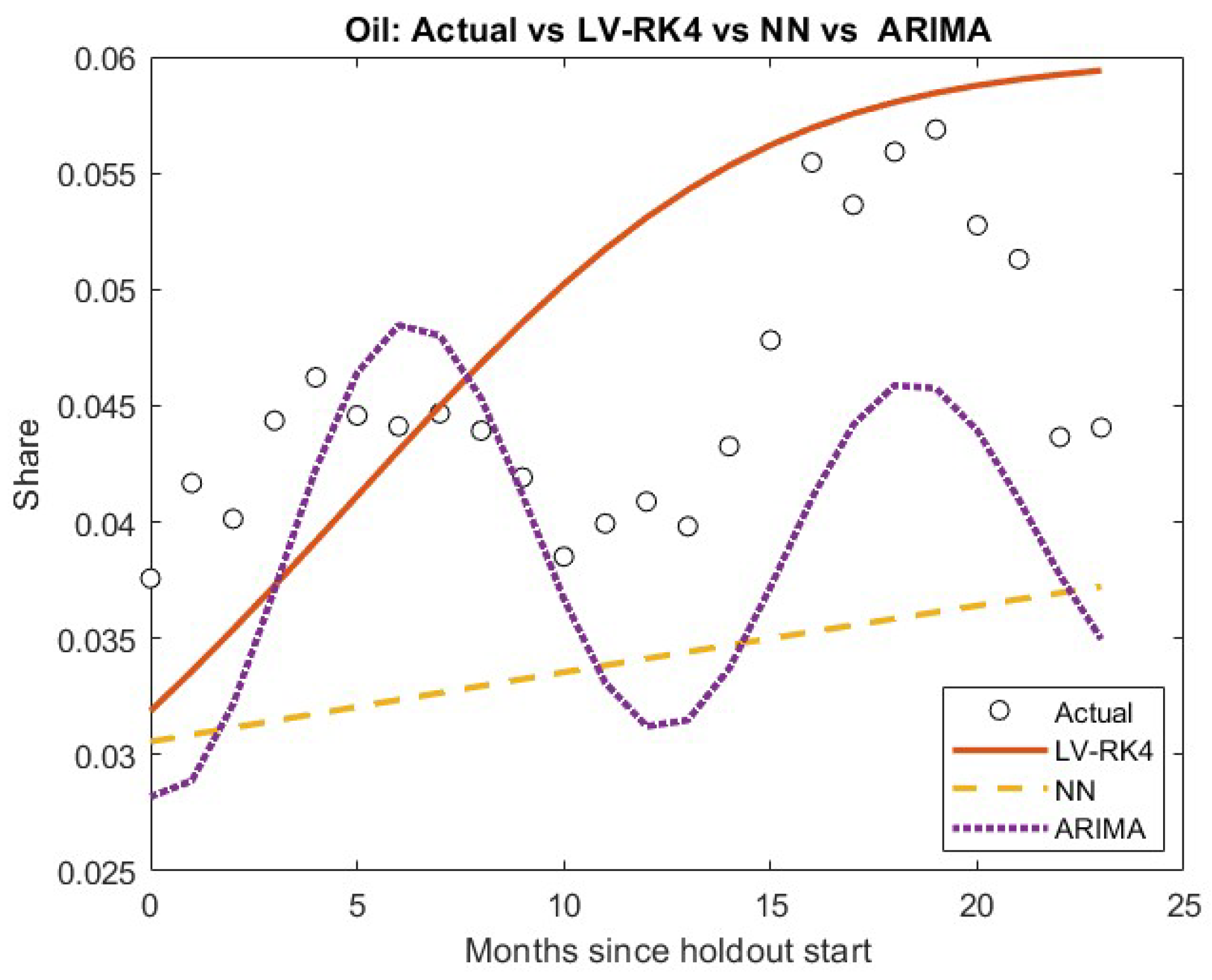
The largest improvements are observed for coal and gas, which are also the more variable components of the system. For coal, the LV–RK4 model reduces the RMSE to $0.03807$, compared with $0.05678$ for the NN baseline and $0.07350$ for ARIMA. For gas, the corresponding RMSE values are $0.03253$, $0.04466$, and $0.06229$. For oil, all three methods perform relatively well, reflecting the smoother dynamics of that component; here the LV–RK4 and ARIMA forecasts are very close in RMSE ($0.00830$ and $0.00832$, respectively), while the NN baseline remains less accurate.

Taken together, these results suggest that the LV layer acts as a useful stabilizing mechanism during extrapolation. In the present dataset and under the reported chronological holdout design, the hybrid NN–LV–RK4 pipeline delivers the best overall forecasting accuracy while preserving the structural interpretability of the interaction coefficients.

Simplex diagnostics on forecasts: Over the holdout window, the (NN diagnostic) trajectories exhibited mean $\left|{\sum }_i{u}_i\left(t\right)-1\right|=6.8414\times {10}^{-4}$ and maximum $1.8580\times {10}^{-3}$, and the number of months with any $u_i\left(t\right)<0$ was 0 and with any $u_i\left(t\right)>1$ was 0.

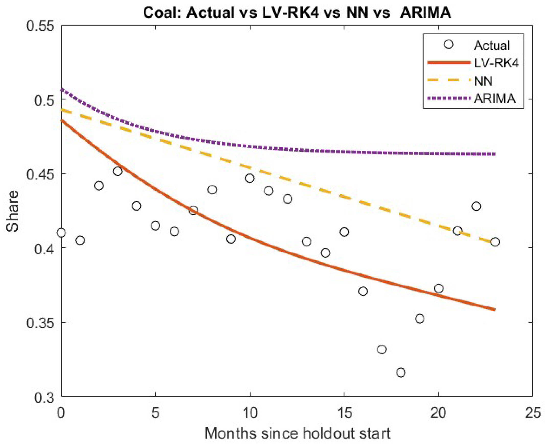
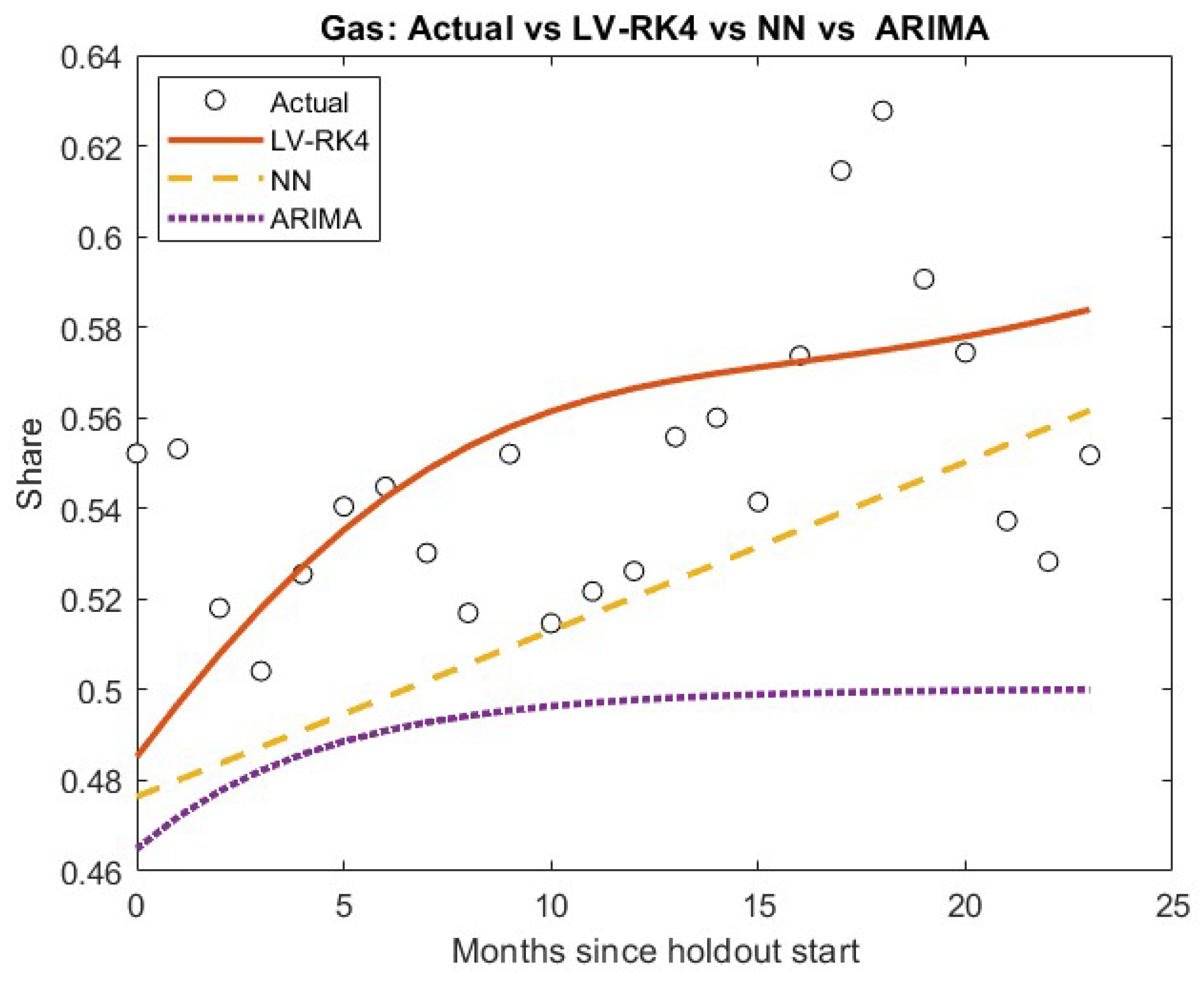
Figure 3, Figure 4 and Figure 5 provide a visual comparison on the holdout window for each component, showing the observed shares together with the ODE-based forecasts, the NN-only forecasts, and the ARIMA benchmark forecasts. The hybrid model follows the medium-horizon movements more consistently, whereas both the NN and ARIMA baselines tend to deviate more strongly when the series changes direction or when reallocations among components occur over a short span of months. This behavior is consistent with the fact that the NN-only approach is an unconstrained function approximator and ARIMA is a univariate statistical benchmark, while the hybrid approach forces the forecast to evolve according to a low-dimensional dynamical system whose parameters are fitted from the NN-implied derivatives.

5.2. Interpretation Through Dynamical Consistency

The proposed pipeline fits a generalized Lotka–Volterra interaction model using derivatives obtained from the trained network and then uses RK4 integration to generate out-of-sample trajectories. From a forecasting perspective, this step is not only a numerical convenience but a modeling choice: it restricts the forecast to trajectories that are dynamically consistent with the fitted interaction structure. The observed reduction in holdout error suggests that this restriction helps prevent unstable extrapolation and improves forecast smoothness without sacrificing the ability to capture the main reallocations among coal, gas, and oil.

5.3. Summary

On the chronological holdout window, the LV–RK4 framework outperforms both the NN-only baseline and the ARIMA benchmark in overall forecasting accuracy, as measured by the RMSE and MAE, with the largest gains observed for coal and gas. In addition, the calibrated ODE model offers a structured simulator for counterfactual experiments, enabling a controlled analysis of shock propagation and reallocation patterns within the three-share system.

In all three cases, the proposed LV–RK4 forecast follows the overall direction of the data more closely than both the NN-only baseline and the ARIMA benchmark, with the difference being especially visible for coal and gas, where the shares exhibit larger month-to-month variation. The ARIMA trajectories tend to remain less responsive to the joint competitive dynamics of the system and therefore deviate more noticeably over the holdout horizon, particularly for the more variable components. For oil, all three methods track the series reasonably well because the dynamics are smoother, although the hybrid forecast remains comparably stable over the horizon. These figures therefore complement the error metrics in Table 3 by showing not only the magnitude of the forecast errors but also the way the competing models capture the shape and temporal evolution of each series.

6. Discussion and Future Research

This study grew out of a practical modeling difficulty we encountered while working with monthly compositional energy share series. Purely neural forecasts can fit the training period very well, but once they are pushed into a genuine holdout window, their trajectories may drift in ways that are hard to justify from the perspective of a constrained share system. The central question, therefore, was whether a data-driven neural estimator could be used to recover smooth trajectories and derivatives, while a low-dimensional dynamical system could provide the structure needed for more stable extrapolation.

Within the chronological holdout experiment reported here, the hybrid NN–LV–RK4 pipeline performs better than both comparison benchmarks considered in this study: the NN-only baseline and the ARIMA$(2,0,2)$ benchmark. The gains are the clearest for coal and gas, which are also the more variable components of the system, while oil is comparatively easy to forecast for all three methods. Importantly, this improvement does not come from adding a more complicated forecasting layer at the final stage. Once the LV parameters have been identified, forecasting reduces to a forward simulation of a compact three-dimensional dynamical system. In that sense, the advantage of the hybrid approach appears to come less from raw flexibility and more from the way the dynamical layer regularizes extrapolation.

In practice, one of the most delicate parts of the pipeline was not training the neural network itself but extracting derivative information that was stable enough to support the second-stage parameter fit. Monthly data are noisy, the sample is short, and small wiggles in the NN trajectories can translate into noticeably different derivative estimates. This sensitivity becomes immediately visible when the derivatives are passed into the least-squares LV identification step: some coefficients, especially weaker cross-effects, can respond strongly to local fluctuations unless the training procedure is stabilized. The moving-block bootstrap was introduced for exactly this reason. It does not eliminate short-sample instability, but in our experiments, it reduced the dependence of the final parameter estimates on a single realization of the training window and made the identification stage more reliable.

A second practical observation is that the LV structure acts as a useful inductive bias. The NN has enough flexibility to track nonlinear patterns over the training window, but direct NN extrapolation can amplify noise when forecasting beyond the last observed point. By converting the NN-implied derivatives into a calibrated LV system, we restrict trajectories to evolve through a small number of interpretable interaction channels. This restriction is the most helpful precisely where the unconstrained forecasts are the most fragile, namely for the more volatile coal and gas shares. The ARIMA benchmark reinforces this point from a different angle: although it provides a reasonable classical statistical reference, it is clearly less effective in representing the joint competitive dynamics of the three fossil components over the holdout period.

The estimated coefficients also offer a compact qualitative picture of substitution and competition among coal, gas, and oil. The signs of several interaction terms are economically plausible and consistent with the idea that shifts in relative costs, policy pressure, and system conditions can redistribute shares across fuels. At the same time, the uncertainty analysis makes clear that not all coefficients are equally well determined by the data. In our experiments, the weaker cross-effects were the first to become unstable across fits, especially where the corresponding component exhibited relatively limited variation. We view this not only as a limitation but also as a useful diagnostic feature of the framework: it helps distinguish interaction patterns that are supported relatively consistently from those that remain only weakly identified.

Several limitations became clear during the implementation of the framework. First, the monthly sample is short, which constrains identifiability in the second-stage LV fit. This is especially visible in weaker interaction terms, where the confidence intervals are wider and the coefficients should be interpreted cautiously. Second, the benchmark set remains limited. In addition to the NN-only model, we also include ARIMA$(2,0,2)$ as a classical benchmark, but the present paper is still not intended as an exhaustive forecasting competition across all statistical, machine learning, and physics-informed alternatives. Third, the model treats the system as closed and autonomous over the forecast horizon. In practice, fossil fuel generation shares respond to exogenous drivers such as carbon prices, fuel prices, renewable penetration, weather conditions, and policy interventions. These factors are only indirectly reflected in the historical series and do not enter the fitted ODE explicitly, which limits the model’s ability to adapt when the system moves into a new regime. Fourth, the LV coefficients are assumed to be constant over the sample. This is a useful first approximation, but it compresses potentially distinct subperiods into a single average interaction structure. Time-varying or covariate-dependent coefficients would be a more realistic way to represent regime changes. Fifth, the Lotka–Volterra structure imposes a specific functional form on interactions. This is a deliberate trade-off: it improves interpretability and supports counterfactual reasoning, but it may miss nonlinear mechanisms that are present in real energy transitions. A further limitation is that we do not provide a dedicated sensitivity analysis for either key LV coefficients or the numerical step choice. While the RK4 propagation was carried out on the same monthly grid as the observations, a more systematic study of coefficient perturbations and numerical step sensitivity would be useful in future work. Finally, the empirical evaluation relies on a single chronological split. Although this is a realistic forecasting setup, it does not eliminate period-specific effects, and the results should therefore be read as evidence from one holdout exercise rather than as a complete robustness assessment.

A further point concerns uncertainty quantification. The confidence intervals reported for the LV coefficients are conditional on the NN-implied trajectories and derivatives used in the second-stage fit. They do not propagate all sources of uncertainty from the full pipeline, including neural network training variability, bootstrap weight selection, or numerical propagation choices. For this reason, the intervals should be interpreted as local identification diagnostics rather than as full end-to-end uncertainty bands for the entire NN–LV–RK4 procedure. Full uncertainty propagation would require repeated retraining and re-estimation across the whole pipeline and is left for future work.

Future work follows naturally from these observations. One immediate direction is to relax the assumption of time-invariant coefficients. The present model summarizes an average interaction structure over the sample, but one would expect the competitive dynamics of coal, gas, and oil to change across policy and price regimes. Allowing the LV coefficients to evolve gradually over time, or conditioning them on exogenous covariates such as carbon prices, gas prices, weather indicators, or renewable penetration, would be a natural next step. The framework also extends in principle to higher-dimensional compositional systems, for example, by incorporating renewables or storage technologies, although scalability and identifiability would require much more careful treatment in that setting.

From a methodological standpoint, several extensions deserve attention. Rolling-origin validation or alternative chronological splits would help assess robustness more systematically. Local sensitivity analysis for the most influential interaction coefficients would clarify how strongly the forecasts depend on perturbations in the fitted parameters. It would also be useful to compare the present framework with a broader family of hybrid methods, including neural ODEs, physics-informed losses, and recurrent architectures equipped with conservation-type constraints. Such comparisons would help clarify more precisely when an explicit dynamical backbone adds the greatest value.

Overall, the evidence reported here supports a narrower but, in our view, more meaningful conclusion: in this dataset and under the reported holdout design, coupling an NN smoother with a low-dimensional LV system improves forecasting accuracy relative to both the NN-only and ARIMA benchmarks considered while preserving interpretability through explicit interaction coefficients. The framework is therefore best viewed as a compact and transparent hybrid modeling tool for medium-horizon compositional forecasting, rather than as a final or exhaustive solution to the broader problem of energy share prediction under structural change.

7. Conclusions

This paper developed a hybrid neural–dynamical framework for forecasting and interpreting the evolution of monthly EU coal, gas, and oil generation shares. A neural network was used to recover smooth trajectories and implied time derivatives from the data, and these derivative estimates were then used to identify the parameters of a three-dimensional generalized Lotka–Volterra (GLV) system. The calibrated system was propagated forward with a fourth-order Runge–Kutta scheme so that the final forecasts were generated by a compact dynamical model rather than by direct black-box extrapolation alone.

Empirically, the NN–LV–RK4 pipeline performs the best among the three models considered in this study under the reported chronological holdout design. Over the final 30% of the sample, the hybrid forecast achieves a mean RMSE of $0.0263$ and an MAE of $0.0215$, compared with $0.0382$ and $0.0330$ for the NN-only baseline and $0.0480$ and $0.0429$ for the ARIMA$(2,0,2)$ benchmark. The improvement is especially clear for coal and gas, while for oil, all three methods perform relatively well, with the hybrid and ARIMA forecasts being very close. In this sense, the main empirical result is not that the hybrid model wins by adding forecasting complexity at the last stage but that the dynamical layer appears to stabilize extrapolation where direct statistical or neural forecasts are more fragile.

Beyond forecasting accuracy, the fitted GLV coefficients provide a structured way to summarize substitution and competition effects among the three fossil components. Some interaction terms are estimated with relatively clear sign and magnitude, whereas others remain weakly identified, and the uncertainty diagnostics make that distinction visible. This is useful in practice because it separates interaction patterns that are consistently supported by the data from those that should be treated more cautiously.

The contribution of this paper is therefore twofold within the scope actually studied here. First, it shows that coupling an NN smoother with a low-dimensional GLV system can improve holdout forecasting accuracy relative to both the NN-only and ARIMA benchmarks considered. Second, it provides an interpretable interaction map that supports scenario exploration in a way that direct black-box forecasts cannot easily offer. At the same time, the present results should be read with appropriate caution: the sample is short, the validation relies on a single chronological split, the LV system is autonomous with fixed coefficients, and the reported parameter intervals are conditional on the NN-based identification stage rather than full end-to-end uncertainty bands.

One question that emerged repeatedly during the experiments is how to introduce regime sensitivity without losing the transparency of the interaction coefficients. The 2017–2023 period contains distinct price and policy conditions, yet the current model summarizes them through a single time-invariant interaction structure. A natural next step is therefore to examine whether slowly time-varying GLV coefficients, or coefficients conditioned on exogenous covariates such as fuel prices, carbon prices, weather indicators, and renewable penetration, can preserve interpretability while improving robustness across changing regimes. Also, two practical extensions suggested by the present experiments are local sensitivity analysis for the most influential cross-effects and a numerical robustness check under alternative propagation steps.

Overall, the results suggest that this hybrid NN–LV–RK4 formulation is best viewed as a compact and interpretable modeling tool for medium-horizon compositional forecasting. In the dataset studied here, it improves on the benchmark models considered while retaining a structure that is simple enough to inspect, discuss, and use for counterfactual analysis.