A DSGE Framework with Green and Fossil Energy for Kazakhstan

Abstract

This paper constructs and estimates a novel two-sector Dynamic Stochastic General Equilibrium (DSGE) model to analyze the macroeconomics of Kazakhstan’s dual-energy structure, where a large fossil fuel sector coexists with an emerging renewable segment. The model’s key innovation is its integration of an endogenous, depletable oil stock and a dual-inflation Taylor-type rule, which together capture the specific transmission channels between hydrocarbon dependence and green investment. By differentiating between oil-driven and core inflation, the framework quantifies how oil price volatility transmits monetary conditions to the renewable sector. Bayesian estimation, using sectoral data from national accounts, reveals a pronounced asymmetry: oil stock/discovery dynamics and oil revenue fluctuations dominate macroeconomic volatility, while the renewable sector exhibits stable output but remains vulnerable to oil-driven monetary tightening transmitted mainly through indirect channels. The results indicate that Kazakhstan’s ongoing energy transition offers a stabilizing diversification benefit in principle but remains structurally constrained by macroeconomic dynamics and fiscal patterns anchored to hydrocarbon conditions. These findings provide a quantitative basis for designing transition policies that mitigate cross-sector spillovers and support effective diversification in resource-dependent economies.

1. Introduction

Kazakhstan is among the world’s most hydrocarbon-dependent economies. Oil production has long accounted for more than two-thirds of export revenues and a substantial share of fiscal income. Large integrated projects at Tengiz, Kashagan, and Karachaganak shape both the scale and volatility of the oil sector. Public support for fossil fuels also remains significant: recent international assessments [1,2] estimate fossil fuel subsidies at around 6% of GDP. As a result, fluctuations in global oil markets translate rapidly into domestic output, inflation, and exchange rate pressures.

In contrast, the renewable (green) energy sector is at an early but dynamic stage of development. According to the International Energy Agency [3], fossil fuels still provide about 98% of Kazakhstan’s final energy consumption, while non-hydro renewables rose only from 0.1% to 0.7% of final consumption between 2014 and 2020. The investment asymmetry is similarly stark: cumulative investment in major oil megaprojects such as Tengiz, Kashagan, and Karachaganak is estimated at USD 50–80 billion (likely above USD 100 billion when expansions are included) [4,5], whereas total green energy investment to date is about USD 3.7 billion [6,7]. Over the long term, however, the balance may reverse: Kazakhstan’s carbon neutrality pathway requires USD 610–1150 billion in green investment by 2060 [8,9,10,11]. This contrast implies that the green transition can become economically central, yet it is currently exposed to macroeconomic shocks and policy responses driven predominantly by the oil economy [12].

Crucially, Kazakhstan’s hydrocarbon dependence is twofold. The country is simultaneously a fossil fuel-intensive consumer and a major oil exporter dependent on rent revenues. These two roles are deeply linked. Export revenues determine the government’s fiscal space and policy options, while inherited infrastructure creates domestic “carbon lock-in”. Together, these factors form a shared “hydrocarbon ecosystem”—spanning budgets, subsidies, and employment networks—that dictate the pace of the green transition. This dynamic parallels other structural transitions, where legacy systems continue to shape investment incentives and constrain new technologies.

This duality motivates two research questions:

RQ1: How does the expansion of renewable (green) generation affect Kazakhstan’s macroeconomic dynamics and the transmission of energy sector shocks in a dual fossil–renewable economy?

RQ2: Whether the volatility of the oil sector negatively affects the development of green economy through fiscal and monetary channels.

These questions are particularly relevant for Kazakhstan, whose long-term development strategy targets increasing renewables to 15% of total electricity production by 2030 [13] while maintaining the fiscal role of hydrocarbons. For hydrocarbon exporters, this risk is amplified. Key economic tools—such as green subsidies and domestic price controls—are often tied directly to the oil cycle [14,15]. As a result, the green transition is not just a matter of switching energy sources; it is also a complex fiscal challenge, requiring the government to untangle its budget and institutions from oil revenues.

To rigorously address these issues, we estimate a two-sector DSGE model that captures the structural frictions of a dual fossil–renewable economy by interacting a clean (green) block with a fossil (oil) block through relative prices, monetary policy, and an explicit fiscal transfer mechanism. Uniquely, the model’s supply side constrains the oil sector with an endogenous resource stock that evolves through depletion and discoveries. On the nominal side, we use sector-specific New Keynesian Phillips Curves [12]. The oil curve specifically includes “world oil inflation” to capture global price transmission. For monetary policy, we employ a Taylor rule that responds separately to core and oil inflation [16]. Finally, the fiscal block creates an “oil-to-green” channel, where renewable subsidies are tied directly to hydrocarbon rents. Disciplined by eight quarterly observables, including sector-specific inflation and fiscal variables, this framework provides a tractable representation of Kazakhstan’s economy.

Unlike standard energy DSGE models that treat natural resources as exogenous price shocks, this model introduces an endogenous oil stock with a depletion path. We combine this with a dual-energy production structure (green vs. fossil) and a frictional fiscal block, allowing us to capture the feedback loops between resource exhaustion, relative price adjustment, and oil-linked fiscal support that standard models miss. Kazakhstan represents a unique laboratory for the green transition. As a middle-income economy, it faces the specific dilemma of funding the green transition with oil money. Unlike developed importers who tax carbon or wealthy exporters who save in sovereign funds, Kazakhstan’s green subsidies are co-integrated with oil revenues, creating a volatility trap where the funding source is structurally opposed to the policy goal of decarbonization.

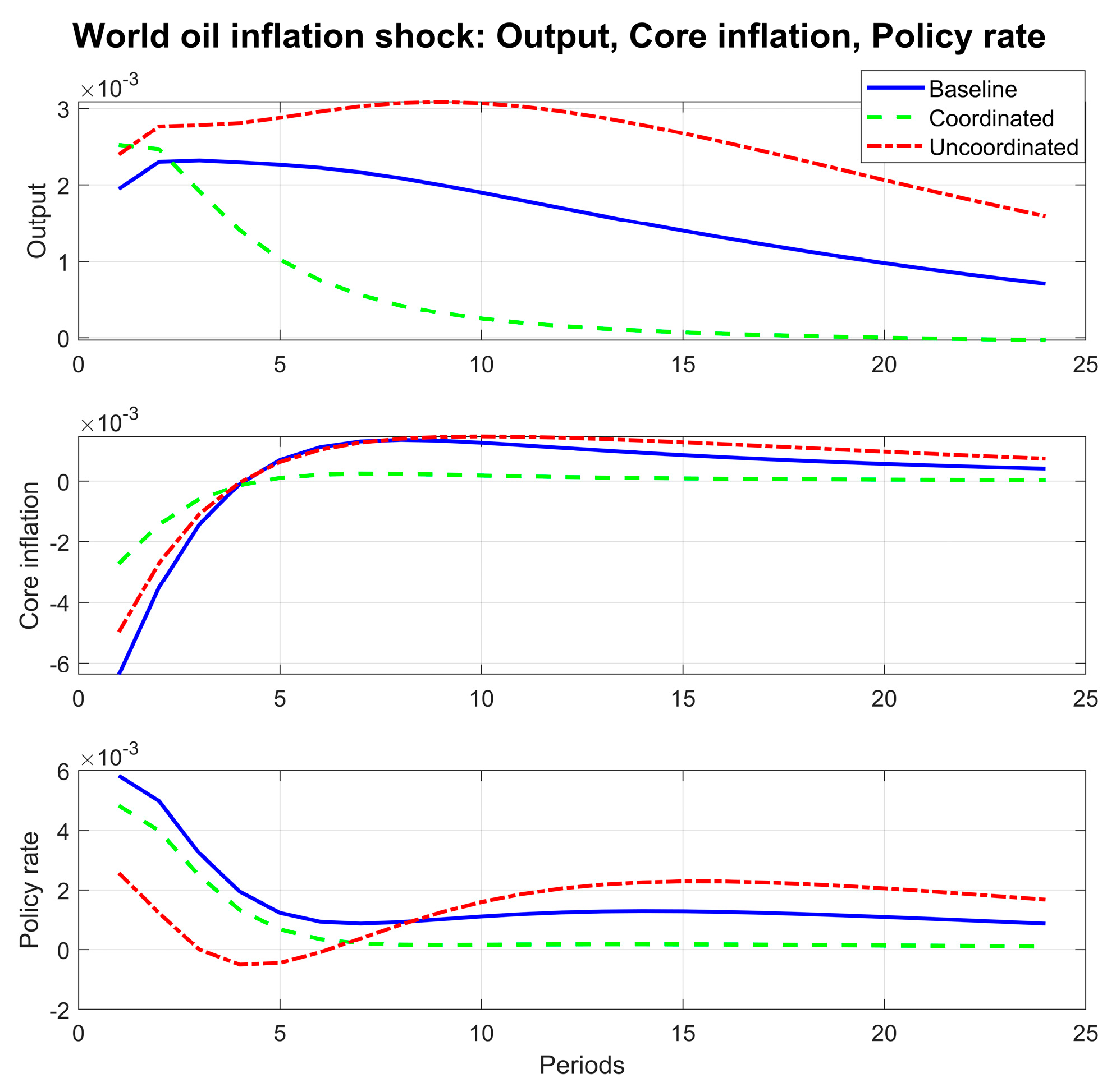
For policymakers, the model demonstrates that aggressive subsidy rules alone are insufficient due to the fiscal resource trap. Our variance decomposition reveals that, while fiscal policy can boost green output in the short run, long-run economic volatility remains determined by the depletion rate. This implies that, without deep structural reforms to decouple fiscal revenues from the oil cycle, green industrial policy will remain hostage to global commodity price fluctuations.

The empirical implementation combines quarterly macroeconomic observables (2010 Q1–2024 Q4) with sectoral energy information used to discipline key priors and calibration targets, including KEGOC statistics and official energy reports (2014–2024) [17]. The estimated parameters characterize the persistence of oil-linked states (oil stock/discoveries, oil revenues, and relative prices), the strength of cross-sector spillovers, and the extent to which transition support is synchronized with the hydrocarbon cycle.

The paper proceeds as follows. Section 2 reviews the related literature. Section 3 presents the model. Section 4, Section 5 and Section 6 describe data, calibration, estimation, and results. Section 7 discusses implications for RQ1 and RQ2, and Section 8 concludes the paper.

2. Literature Review

Existing macro-energy DSGE models provide important theoretical foundations for understanding the interaction between fossil fuels, environmental policy, and the broader macroeconomy. We categorize the relevant literature into three streams: resource-rich macroeconomics, energy transition models, and country-specific studies, highlighting the gap that our specific dual-energy framework addresses.

2.1. Resource-Rich DSGE Models

The first strand focuses on macroeconomic management of exhaustible resources. The benchmark reference is Medina and Soto [18], who developed a copper sector DSGE for Chile. Their results quantitatively demonstrate that a structural fiscal rule could reduce the output response to a 10% commodity price shock from 0.7% to 0.05%, proving the stabilizing power of fiscal anchors. This line of inquiry is supported by the Norwegian fiscal analysis model NORA [19], where Aursland et al. [20] show that the “Bird-in-Hand” rule almost fully insulates GDP from oil price volatility, though at the cost of greater financial exposure.

Comparative evidence further underscores the role of institutions. Pieschacón [21] compared Mexico and Norway, finding that “Norwegianizing” Mexico would dramatically reduce volatility, implying that fiscal institutions drive stability more than the resource structure itself. In the context of Russia, Andreev [22] found a trade-off: while fiscal rules stabilize the real exchange rate, they may lead to higher volatility in inflation and interest rates. Regarding monetary policy, Allegret and Benkhodja [23] modeled Algeria and showed that targeting core inflation yields higher welfare than Consumer Price Index (CPI) targeting in the presence of dominant oil shocks. Similarly, for Nigeria, Adebiyi and Mordi [24] estimate a remarkably low exchange rate pass-through (≈0.1), attributing it to improved monetary policy credibility. Finally, Tavakolian et al. [25] highlight the importance of distinguishing shock types: while oil technology shocks expand production, they can contract the non-oil sector through Dutch disease effects [26], whereas price shocks primarily affect nominal variables.

2.2. Energy Transition DSGE Models

The second strand integrates environmental policy and renewable sectors. Early theoretical contributions, such as Golosov et al.’s [27], focused on optimal carbon taxation derived from intertemporal efficiency conditions. New Keynesian extensions, like Annicchiarico and Di Dio’s [28], analyze how environmental instruments interact with nominal rigidities and monetary rules.

More recent applied work explicitly models the transition between sectors. Argentiero et al. [29] estimate a two-energy DSGE for the Euro Area, finding that renewable-support policies affect macro conditions primarily through energy cost channels. Large-scale multi-sector models, such as the Bundesbank’s EMuSe [30], add significant sectoral detail but typically assume diversified energy mixes typical of advanced economies rather than the monopolistic fossil dominance of oil exporters. Furthermore, Boehl, Budianto, and Takáts [31] show that taxing “brown” energy induces sizable inflationary and output effects, while Chan et al. [32] emphasize the role of green credit and macroprudential tools in managing transition risks. However, a key limitation in this literature is that these models rarely incorporate the endogenous depletion of fossil reserves or the specific transmission channels relevant to a small open economy like Kazakhstan’s.

2.3. Kazakhstan-Specific Studies

The third strand documents the specific context of Kazakhstan. System-level assessments describe a power mix where fossil fuels still provide approximately 98% of consumption, coexisting with ambitious decarbonization targets [13,33,34]. Empirical studies have analyzed regulatory challenges, including tariff design and investment risks in the renewable segment [35,36,37], as well as the spatial potential for renewable generation [38,39,40]. Recent work on investment trends documents that, while renewable investment is accelerating, it remains modest relative to the fossil sector [41,42,43].

Macroeconomic modeling for Kazakhstan has evolved significantly. Abilov [44] estimates a Bayesian DSGE finding that risk-premium shocks explain almost 60% of tenge exchange rate volatility. Algozhina [45] provides a normative analysis demonstrating that countercyclical fiscal rules combined with exchange rate flexibility constitute the welfare-maximizing regime. Konebayev [46] adapted the Medina-Soto framework, revealing asymmetric responses where oil shocks became contractionary during the 2007 and 2015 crises. Most recently, the National Bank of Kazakhstan has begun developing models that account for differentiated labor supply and wage rigidity [47], while Akhmedyarova [48] integrates the housing sector to explain consumption fluctuations.

To sum up, existing macro-energy DSGE research falls into three main streams and motivates a gap that a dual-energy, small open-economy framework with fossil depletion can fill. Resource-rich DSGE models study how to manage exhaustible resource shocks through policy rules and institutions. Chilean and Norwegian benchmark models show that fiscal anchors can strongly dampen output responses to commodity price shocks. Cross-country comparisons stress that institutional design (especially fiscal frameworks) matters more for volatility than resource endowments themselves. For oil exporters such as Russia, Algeria, and Nigeria [49], the literature highlights policy trade-offs: fiscal rules can stabilize the exchange rate but may raise inflation and interest rate volatility; monetary regimes perform better when targeting core inflation rather than headline CPI; credibility can lower exchange rate pass-through [50]. A recurring message is that shock identification is crucial: technology shocks and price shocks propagate differently, and oil shocks can trigger Dutch disease reallocation that hurts the non-resource sector. What is largely missing from this literature is a unified quantitative framework that embeds both fossil and renewable generation into a single DSGE model calibrated to economies’ specific dual structure. Existing resource-rich models typically treat energy as a single block, while transition models often abstract from the exhaustible nature of the resource. By developing a two-sector framework with endogenous oil depletion, cross-sector price dynamics, and an asymmetric monetary policy rule, this paper aims to bridge these streams.

The main contributions can be summarized along three dimensions. First, unlike standard DSGE models for resource-rich economies, this paper treats oil reserves as a depletable stock that evolves over time through extraction and discoveries. This means the oil sector is not driven only by external price or revenue shocks, but also by a physical resource constraint that links current production to future capacity. Second, the model highlights a key contradiction in Kazakhstan’s transition path: oil revenues provide the fiscal resources needed to support green development, but because that support depends on oil income, it becomes unstable whenever oil prices or oil revenues fluctuate. Third, compared with existing DSGE applications for Kazakhstan, the paper jointly estimates oil depletion dynamics, an oil revenue-based subsidy rule, and a monetary policy rule that responds separately to core inflation and oil inflation. Taken together, the paper’s main contribution is to show that oil shocks can play a dual role: they can create fiscal space for green support, but they can also show diversification by tightening monetary conditions and making transition financing more volatile.

3. Model Overview

This paper develops a Dynamic Stochastic General Equilibrium (DSGE) model tailored to the unique structure of Kazakhstan’s economy. The developed DSGE framework represents a small open economy with two distinct production blocks—a fossil fuel sector and a clean energy sector—that interact through unique supply-side constraints and nominal rigidities. In this paper, the non-oil sector represents the green economy in the model. Accordingly, we use the terms non-oil, clean, and green sector interchangeably. A primary theoretical innovation lies in the specification of the oil sector. Rather than treating oil production solely as an instantaneous flow, we constrain it using a conservation-consistent, endogenous oil stock that evolves dynamically through extraction and new discoveries. This formulation introduces a critical “slow-moving state” variable into the system, ensuring that shocks to the oil sector generate structural persistence that extends well beyond transient price fluctuations. On the nominal dimension, the model incorporates sector-specific New Keynesian Phillips Curves to distinguish between core and energy price dynamics. Crucially, the oil inflation curve is augmented with an exogenous “world oil inflation” component, a modification that allows the model to capture the high pass-through of global commodity variance into domestic prices. To manage this external volatility, the monetary authority is modeled with a dual-target Taylor rule, reacting separately to core and oil inflation to prevent sector-specific shocks from destabilizing the aggregate economy.

To rigorously operationalize the institutional challenges of the green transition, the model embeds a fiscal transfer mechanism that explicitly couples renewable energy support to the hydrocarbon cycle. Green subsidies are governed by a persistent policy rule that loads positively on oil revenues, thereby creating a pro-cyclical feedback loop where financing for the transition remains vulnerable to the volatility of fossil fuel markets. Complementing this, the oil revenue process itself is modeled to reflect both domestic extraction volumes and exogenous global price shocks. The empirical validity of the system is established using eight specific observables—including disaggregated inflation rates, fiscal oil revenues, and subsidy costs. This rich data structure allows for the joint identification of the two dominant forces in the Kazakh economy: the structural inertia imposed by the physical oil stock and the financial fragility introduced by the oil-to-green funding channel. The goal is to provide a quantitative framework to simulate the effects of various shocks and policies on key macroeconomic variables like output and inflation in both sectors.

We decompose inflation into core and oil-driven components following Aoki and Bodenstein et al. [51,52]. We allow relative oil price shocks to pass through to core inflation via the marginal cost channel, capturing the supply-side inflationary pressure of oil shock. This distinction is structurally motivated by the heterogeneity in price-setting behavior: while core prices are governed by domestic nominal rigidities (sticky prices), the energy component is driven by flexible, globally determined commodity prices. Unlike generic markup shocks, which serve as unobservable residuals, this decomposition allows us to explicitly model the pass-through of observable exogenous world oil inflation ${\pi }_{oil}^{*}$ into the domestic economy, thereby isolating the specific transmission mechanism of external terms-of-trade shocks that is distinct from domestic demand pressures.

To capture the heterogeneity in monetary transmission, we employ a disaggregated Taylor rule that responds separately to core and oil inflation. By allowing distinct coefficients, we aim to empirically identify whether the central bank differentiates between domestic inflationary pressures (driven by demand) and exogenous terms-of-trade shocks (driven by global commodity markets).

We model the oil sector’s production dynamics following the endogenous reserves framework of Gross and Hansen [53] to capture the deep-seated structural inertia of Kazakhstan’s hydrocarbon ecosystem. Unlike standard models that treat natural resources as exogenous income flows, our framework recognizes that the oil sector operates under an intertemporal resource constraint: current extraction depletes the finite stock, while discoveries generate persistent wealth shocks that alter long-run fiscal and consumption paths. By formalizing the oil stock as a slow-moving state variable, we introduce “systemic memory” into the model, ensuring that energy shocks are not merely transitory price blips but are propagated over time through the physical depletion–discovery cycle. This specification essentially provides a physical representation of the “fossil lock-in”: it depicts an economy where macroeconomic stability is structurally anchored to geological reserves, creating a massive, capital-intensive ecosystem that inherently resists rapid diversification regardless of short-term price signals.

To isolate the specific transmission mechanisms of the hydrocarbon–fiscal feedback loop, the model intentionally abstracts from aggregate capital accumulation, nominal exchange rate frictions, and wage rigidities. By treating non-oil physical capital as fixed in the short run, we force the dynamics of the system to be driven entirely by the endogenous oil stock, thereby highlighting the role of natural resource depletion as the primary intertemporal constraint. Similarly, we capture external competitiveness through real terms of trade (the relative price of oil) rather than explicit nominal exchange rate modeling, effectively filtering out unconnected Uncovered Interest Parity (UIP) shocks.

3.1. Household Sector

Optimization Problem

The model begins with a representative household that makes decisions about consumption and labor supply. This household seeks to maximize its expected lifetime utility, which depends positively on consumption and negatively on the effort of work. The representative household maximizes expected lifetime utility:

$$\mathrm{m}\mathrm{a}\mathrm{x}{E}_0\sum _{t=0}^{\mathrm{\infty }}{\beta }^t\left[{\displaystyle \frac{{\left(C_t-h{C}_{t-1}\right)}^{1-\sigma }}{1-\sigma }}-{\displaystyle \frac{N_t^{1+\varphi }}{1+\varphi }}\right]$$

(1)

where C_t and C_t−1 are consumption at time t and the previous period, respectively. N_t is labor supply at time t. Parameter $\beta$ is the discount factor, which captures the household’s preference for immediate consumption over future consumption; a value less than one reflects patience. The habit formation parameter $h\in \left(0,1\right)$ measures the degree to which current utility depends on past consumption. The coefficient $\sigma$ governs the household’s relative risk aversion and the desire for smooth consumption over time. A higher $\sigma$ makes the household more averse to fluctuations in consumption. Finally, $\varphi$ is the inverse of the Frisch elasticity, determining how sensitively labor supply responds to changes in real wage.

To maximize its utility, the household is constrained by its budget. It cannot spend more than its total income in any given period. That is,

$$P_{c,t}{C}_t+B_t=W_t{N}_t+R_{t-1}{B}_{t-1}+V_t+T_t$$

(2)

where P_c,t is the price of consumption goods at time t, $C_t$ is the household consumption, $B_t$ denotes bonds purchased in period t, $W_t$ is the wage rate, $N_t$ is the labor supplied by the household, $R_{t-1}$ is the gross return on bonds purchased in the previous period, $B_{t-1}$ is the stock of bonds carried from period t − 1, $V_t$ represents profits or dividends distributed to households, and $T_t$ denotes government transfers received by the household.

This budget constraint states that the household’s spending on consumption goods ($P_{c,t}{C}_t$) and the purchase of new financial bonds ($B_t$), which are a means of saving, must equal its total income. Income comes from wages earned from labor ($W_t{N}_t$), the return on bonds purchased in the previous period ($R_{t-1}{B}_{t-1}$), profits distributed from firms ($V_t$), and government transfers ($T_t$). In the context of Kazakhstan, this captures the flow of income from both the oil and non-oil sectors to households.

To solve this constrained optimization problem, we set up a Lagrangian. The first-order conditions derived from this Lagrangian describe the household’s optimal behavior.

First-order conditions:

The Lagrangian for the household problem is:

$$\mathcal{L}=E_0\sum _{t=0}^{\mathrm{\infty }}{\beta }^t\left\{{\displaystyle \frac{{\left(C_t-h{C}_{t-1}\right)}^{1-\sigma }}{1-\sigma }}-{\displaystyle \frac{N_t^{1+\varphi }}{1+\varphi }}+{\lambda }_t\left[W_t{N}_t+R_{t-1}{B}_{t-1}+V_t+T_t-P_{c,t}{C}_t-B_t\right]\right\}$$

(3)

The Euler equation is:

$${\lambda }_t=\beta E_t\left[{\lambda }_{t+1}{R}_t{\displaystyle \frac{P_{c,t}}{P_{c,t+1}}}\right]$$

(4)

The Euler equation is a fundamental condition in intertemporal economics. It describes the optimal path for consumption and saving. Here, ${\lambda }_t$ is the Lagrange multiplier, representing the marginal utility of wealth (or the value of an additional unit of income). The equation states that the household will adjust its saving and consumption until the utility cost of saving one more unit today (the left-hand side, ${\lambda }_t$) equals the expected discounted utility benefit of consuming the proceeds of that saving tomorrow (the right-hand side). The term $R_t{\displaystyle \frac{P_{c,t}}{P_{c,t+1}}}$ is the gross real interest rate, converting nominal bond returns into future consumption units. For Kazakhstan, this equation helps determine how domestic saving responds to changes in interest rates and inflation expectations.

The labor supply is:

$$W_t=N_t^{\varphi }{\lambda }_t^{-1}$$

(5)

This equation defines the household’s labor supply decision. It states that the nominal wage ($W_t$) must equal the marginal disutility of work ($N_t^{\varphi }$) divided by the marginal utility of consumption (${\lambda }_t$). In essence, it describes the real wage ($W_t/P_{c,t}$) required to induce the household to supply a given amount of labor. When the marginal utility of consumption is high (e.g., during a recession), the household is willing to work for a lower real wage.

The marginal utility of consumption is:

$${\lambda }_t={\left(C_t-h{C}_{t-1}\right)}^{-\sigma }-\beta h{E}_t{\left(C_{t+1}-h{C}_t\right)}^{-\sigma }$$

(6)

where all variables in this expression follow the same definitions provided in the household’s utility function above (Equation (1)).

This Equation (6) explicitly defines the marginal utility of consumption (${\lambda }_t$) in terms of current, past, and expected future consumption. It shows that with habit formation ($h>0$), marginal utility depends not only on current consumption but also on how it relates to past consumption and future expectations. In the operational DSGE model, we follow standard practice in the New Keynesian literature by implementing a “cashless economy” framework. This approach solves equilibrium allocations using the first-order conditions derived above, while the budget constraint is satisfied via Walras Law in equilibrium [54]. Specifically, we assume bonds are in zero net supply ($B_t=0$), firms operate competitively with zero profits ($V_t=0$), and government transfers ($T_t$) adjust to satisfy the consolidated government budget. These standard simplifications allow the model to focus on the core transmission channels while maintaining theoretical consistency.

3.2. Firms

3.2.1. Non-Oil Sector

Firms in the non-oil sector produce goods and services using a standard Cobb–Douglas production technology. The equation

$$Y_{c,t}=A_{c,t}{N}_{c,t}^{{\alpha }_c}{K}_{c,t}^{1-{\alpha }_c}$$

(7)

states that non-oil output ($Y_{c,t}$) is produced by combining labor ($N_{c,t}$) and capital ($K_{c,t}$), with efficiency determined by the sector’s Total Factor Productivity ($A_{c,t}$). The parameter ${\alpha }_c$ is the labor share of income, indicating the portion of output paid to workers. For the short-run analysis, capital is often assumed to be fixed, making labor the primary variable input. In the context of Kazakhstan’s transition, improvements in $A_{c,t}$ (green Total Factor Productivity (TFP)) could represent technological breakthroughs in renewable energy or efficiency gains.

Firms in this sector are price-takers in the input market and minimize their costs. The first-order condition from this minimization problem yields the labor demand curve. Equation (8),

$$W_t=M{C}_{c,t}{\alpha }_c{A}_{c,t}{N}_{c,t}^{{\alpha }_c-1}{K}_{c,t}^{1-{\alpha }_c},$$

(8)

states that a profit-maximizing firm will hire labor up to the point where the nominal wage ($W_t$) equals the value of the marginal product of labor. The term ${\alpha }_c{A}_{c,t}{N}_{c,t}^{{\alpha }_c-1}{K}_{c,t}^{1-{\alpha }_c}$ is the marginal product of labor—the extra output from one more unit of labor—and $M{C}_{c,t}$ is the nominal marginal cost of production. This relationship is key to understanding employment dynamics in the non-oil sector.

The exact marginal cost for a specific firm in the clean sector, relating it to current wages, available technology, and the fixed stock of capital is presented below:

$$M{C}_{c,t}\left(i\right)={\displaystyle \frac{W_t}{{\alpha }_c{\overline{A}}_{c,t}{K}_c^{1-{\alpha }_c}}}{\left({\displaystyle \frac{Y_{c,t}\left(i\right)}{{\overline{A}}_{c,t}{K}_c^{1-{\alpha }_c}}}\right)}^{{\displaystyle \frac{1-{\alpha }_c}{{\alpha }_c}}}$$

(9)

The first fraction represents the baseline cost of labor per unit of effective capital, while the second bracketed term scales this cost based on the firm’s output level. The exponent on the output term captures the law of diminishing returns, indicating that, as the firm increases production while capital remains fixed, the cost to produce each additional unit grows effectively higher. Its log_linear form is presented below:

$$m{c}_{c,t}=w_t-{\displaystyle \frac{1}{{\alpha }_c}}{a}_{c,t}-{\displaystyle \frac{{\alpha }_c-1}{{\alpha }_c}}{y}_{c,t}$$

(10)

3.2.2. Oil Sector

The oil sector has a distinct production structure that explicitly accounts for the exhaustible nature of the resource. Equation (11),

$$Y_{oil,t}=A_{oil,t}{N}_{oil,t}^{{\alpha }_{oil}}OilStoc{k}_t^{1-{\alpha }_{oil}},$$

(11)

shows that unlike the clean sector, oil production ($Y_{oil,t}$) uses labor ($N_{oil,t}$) and the available stock of oil reserves ($OilStoc{k}_t$) as inputs. The parameter ${\alpha }_{oil}$ is the labor share in oil extraction. This specification captures a key feature of resource-rich economies like Kazakhstan: production is constrained by the finite resource base. The term $OilStoc{k}_t^{1-{\alpha }_{oil}}$ implies decreasing returns to scale for a given stock, meaning that simply adding more labor will not proportionally increase output if the resource base is fixed. Productivity $A_{oil,t}$ can capture factors like extraction technology and geopolitical disruptions.

The labor demand in the oil sector is derived similarly through cost minimization.

$$W_t=M{C}_{oil,t}{\alpha }_{oil}{A}_{oil,t}{N}_{oil,t}^{{\alpha }_{oil}-1}OilStoc{k}_t^{1-{\alpha }_{oil}}$$

(12)

This condition is analogous to that in the clean sector but incorporates the oil stock. It highlights how the productivity of labor in the oil sector, and hence the wage it can pay, is directly linked to the size of the remaining resource base.

$$M{C}_{oil,t}\left(i\right)={\displaystyle \frac{W_t}{{\alpha }_{oil}}}\cdot {\displaystyle \frac{1}{A_{oil,t}}}\cdot {\left({\displaystyle \frac{Y_{oil,t}\left(i\right)}{A_{oil,t}}}\right)}^{{\displaystyle \frac{1-{\alpha }_{oil}}{{\alpha }_{oil}}}}\cdot OilStoc{k}_{t-1}^{-{\displaystyle \frac{\left(1-{\alpha }_{oil}\right)\left({\alpha }_{oil}+1\right)}{{\alpha }_{oil}}}}$$

(13)

In the log-linearized form, the real marginal cost for the oil sector is given by:

$$m{c}_{oil,t}=w_t-s_{oil,t}-{\displaystyle \frac{1}{{\alpha }_{oil}}}{a}_{oil,t}-{\displaystyle \frac{{\alpha }_{oil}-1}{{\alpha }_{oil}}}{y}_{oil,t}-{\displaystyle \frac{1-{\alpha }_{oil}}{{\alpha }_{oil}}}oilstoc{k}_t$$

(14)

The expression shows that marginal cost depends positively on the real wage and negatively on the output due to diminishing returns to labor.

Price-setting: Calvo mechanism to introduce nominal rigidities—a cornerstone of New Keynesian economics—the model uses the Calvo [55] mechanism. In each period, only a random fraction of firms in each sector ($1-{\theta }_c$ and $1-{\theta }_{oil}$) are allowed to adjust their prices optimally.

3.2.3. Clean Sector Phillips Curve

Equation (15) presents the New Keynesian Phillips Curve for the clean sector.

$${\pi }_{c,t}=\beta E_t{\pi }_{c,t+1}+{\kappa }_{c}m{c}_{c,t}+{\mu }_{c,t}$$

(15)

It states that current inflation in the clean sector (${\pi }_{c,t}$) depends on expected future inflation ($E_t{\pi }_{c,t+1}$) and the real marginal cost ($m{c}_{c,t}$) in that sector. The parameter ${\kappa }_c={\displaystyle \frac{\left(1-{\theta }_c\beta \right)\left(1-{\theta }_c\right)}{{\theta }_c}}$ determines how strongly real costs pass through to prices; a higher ${\theta }_c$ (more price stickiness) leads to a flatter Phillips curve (lower ${\kappa }_c$). The term ${\mu }_{c,t}$ is a “cost-push shock”, representing other factors that affect pricing decisions, such as changes in markups or indirect taxes. This equation is vital for analyzing inflation dynamics in Kazakhstan’s non-oil economy.

3.2.4. Oil Sector Phillips Curve

Similarly, for the oil sector with Calvo probability ${\theta }_{oil}$, we have:

$${\pi }_{oil,t}=\beta E_t{\pi }_{oil,t+1}+{\kappa }_{oil}m{c}_{oil,t}+{\mu }_{oil,t}+{\pi }_{oil,t}^w$$

(16)

where ${\pi }_{oil,t}=\mathrm{l}\mathrm{o}\mathrm{g}\left(P_{oil,t}/P_{oil,t-1}\right)$ is oil inflation, ${\kappa }_{oil}={\displaystyle \frac{\left(1-{\theta }_{oil}\right)\left(1-\beta {\theta }_{oil}\right)}{{\theta }_{oil}}}$, ${\mu }_{oil,t}$ is an oil cost-push shock, and ${\pi }_{oil,t}^w$ is an exogenous world oil inflation component that captures external commodity price pressures.

A similar Phillips curve governs inflation in the oil sector. The different Calvo parameter (${\theta }_{oil}$) allows for the possibility that oil prices are more or less flexible than prices in the clean sector, which is a realistic feature given the global nature of commodity markets.

Kazakhstan’s economy relies on finite hydrocarbon reserves, creating critical intertemporal trade-offs. Unlike standard models that treat oil merely as an exogenous flow, we incorporate an endogenous oil stock and a dynamic depletion equation. This captures the structural reality that current extraction permanently reduces future productive capacity, a mechanism often overlooked in conventional DSGE frameworks.

We specify an oil production function dependent on proven reserves, $OilStoc{k}_t$. Unlike reproducible capital, this stock is modeled as a depletable asset, implying that current extraction explicitly constrains future production potential.

Crucially, this stock evolves according to:

$$OilDis{c}_t={\rho }_{oildisc}OilDis{c}_{t-1}+{\epsilon }_{oildisc,t}$$

(17)

$$OilStoc{k}_t=OilStoc{k}_{t-1}-Y_{oil,t}+Oildis{c}_t.$$

(18)

The log-linear form is:

$$oilstoc{k}_t=oilstoc{k}_{t-1}-{\delta }_{oil}{y}_{oil,t}+oildis{c}_t$$

(19)

where ${\delta }_{oil}\equiv {\displaystyle \frac{Q^{ss}}{O^{ss}}}.$ In Section 4 we calibrate ${\delta }_{oil}$ using the observed reserves-to-production ratio (R/P), providing a data-based depletion rate consistent with the oil stock law of motion.

This specification captures two key features of Kazakhstan’s oil economy:

• Endogenous depletion dynamics that create an intertemporal trade-off between current income and future productive capacity.
• Stock-flow consistency in modeling the hydrocarbon sector, moving beyond treating oil as a simple exogenous income stream to capture its finite nature and reserve dynamics.

Our oil stock law of motion captures the intertemporal nature of depletion in a reduced form: higher extraction today lowers the reserve stock available tomorrow, while discoveries partially relax this constraint. In this sense, the remaining reserve stock carries an implicit scarcity value, because current extraction affects future production possibilities. Although the model does not include a fully explicit intertemporal extraction problem or a separate shadow price equation for reserves, it is consistent with forward-looking oil sector behavior.

3.3. Relative Oil Price

The model tracks the relative prices between the two sectors, which are crucial for resource allocation. Equations (20) and (21) define the log-deviations of sectoral relative prices.

$$s_t={\rho }_s{s}_{t-1}+\left({\pi }_{oil,t}-{\pi }_{c,t}\right)$$

(20)

$$s_t=\mathrm{l}\mathrm{o}\mathrm{g}{S}_t$$

(21)

where ${\rho }_s\in \left[\mathrm{0,1}\right)$ captures persistence in relative price adjustments (e.g., real rigidities or slow pass-through).

The model also includes external demand, recognizing Kazakhstan’s role as a small open economy.

$$y_{c,t}=\left(1-{\alpha }_{c,open}\right)c_t+{\alpha }_{c,open}{c}_{ast,t}-\zeta \hspace{0.17em}{s}_t+g_t+subsid{y}_t$$

(22)

$$y_{oil,t}=\left(1-{\alpha }_{oil,open}\right)oilstoc{k}_t+{\alpha }_{oil,open}oi{l}_{ast,t}+\zeta \hspace{0.17em}{s}_t+g_t$$

(23)

Demand for clean sector output comes from domestic consumption ($C_t$), foreign demand ($C_t^{\mathrm{*}}$), government spending ($G_t$), and is sensitive to its relative price ($s_{c,t}$). Similarly, demand for oil is a function of the resource stock (affecting domestic use and investment), foreign demand ($Oi{l}_t^{\mathrm{*}}$), its relative price, and government demand. The parameters ${\alpha }_c$ and ${\alpha }_{oil}$ represent the openness of each sector to international markets. This structure allows the model to simulate the impact of global economic cycles and commodity price shocks on the Kazakh economy.

3.4. Monetary Policy

The National Bank (NBK) of Kazakhstan is modeled as following an interest rate rule, a common approach for modeling central bank behavior.

$$R_t={\rho }_r{R}_{t-1}+\left(1-{\rho }_r\right)\left({\varphi }_{{\pi }_c}{\pi }_{c,t}+{\varphi }_{{\pi }_{oil}}{\pi }_{oil,t}+{\varphi }_y\left(y_t-y_{t-1}\right)\right)+{\epsilon }_{r,t}.$$

(24)

This Taylor-type rule states that the central bank sets the nominal interest rate ($R_t$) based on a combination of past interest rates (capturing smoothing behavior with parameter ${\rho }_r$), the inflation rates in both the clean and oil sector (${\pi }_{c,t}$ and ${\pi }_{oil,t}$), and the growth rate of aggregate output ($y_t-y_{t-1}$). The coefficients ${\varphi }_{{\pi }_c}$ and ${\varphi }_{{\pi }_{oil}}$ reflect the central bank’s dual focus on core and headline inflation, which is particularly relevant for an oil exporter where headline inflation is heavily influenced by global commodity prices. The shock ${\epsilon }_{r,t}$ represents unanticipated deviations from the rule.

Our dual-inflation Taylor rule is motivated by both theory and Kazakhstan-specific policy practice. On the theory side, models with sectoral relative price shocks imply that monetary policy need not react one-for-one to commodity-driven inflation, because energy price movements often reflect external terms-of-trade shocks rather than purely domestic overheating [51,52]. On the institutional side, the National Bank of Kazakhstan has conducted monetary policy under an inflation-targeting regime since 2015, with price stability as its primary objective and the base rate as its main instrument [56]. The Bank’s policy framework further emphasizes that, in a small open economy exposed to external shocks, decisions are based on macroeconomic analysis and forecasting [56]. Recent base-rate statements also distinguish imported price pressures, such as higher global food and energy prices, from core inflation and domestic demand pressures [57]. We therefore allow separate policy coefficients on core and oil inflation: the specification is theory-guided, but the quantitative weight on oil inflation is determined by the data.

3.5. Fiscal Policy and Resource Revenues

Fiscal policy is linked directly to oil revenues, a key feature of Kazakhstan’s public finance.

$$oilre{v}_t={\rho }_{oilrev}oilre{v}_{t-1}+{\chi }_{rev,poil}{\pi }_{oil,t}^w+{\chi }_{rev,y}{y}_{oil,t}+{\epsilon }_{oilrev,t}$$

(25)

where $oilre{v}_t$ is the log-deviation of real oil revenues, ${\chi }_{rev,poil}$ and ${\chi }_{rev,y}$ are elasticities with respect to world oil inflation and oil output, and ${\epsilon }_{oilrev,t}$ is an oil revenue shock.

Government subsidies to the clean sector are linked to oil revenues:

$$subsid{y}_t={\rho }_{sub}subsid{y}_{t-1}+\left(1-{\rho }_{sub}\right)\left({\psi }_{sub}oilre{v}_t\right)+{\epsilon }_{sub,t}$$

(26)

where $subsid{y}_t$ is the log-deviation of real subsidy spending, ${\rho }_{sub}\in [0,1)$ is persistence, ${\psi }_{sub}\ge 0$ measures the sensitivity to oil revenues, and ${\epsilon }_{sub,t}$ is a subsidy shock.

3.6. Shock Processes

In a Dynamic Stochastic General Equilibrium (DSGE) model, the “stochastic” component is introduced through exogenous shock processes. These are random disturbances that hit the economy and force all agents (households, firms, and the government) to adjust their optimal plans. The model’s dynamics are essentially the story of how the economy responds to and propagates these shocks over time.

Formally, all shocks ${\epsilon }_{i,t}$ are assumed to be independently and identically distributed (i.i.d.) with mean zero and standard deviation ${\sigma }_i$:

$${\epsilon }_{i,t}\sim \mathcal{N}\left(0,{\sigma }_i^2\right), \mathrm{i}.\mathrm{i}.\mathrm{d}. \mathrm{over} t$$

for each shock type $i\in \{a_c,a_{oil},{\mu }_c,{\mu }_{oil},c^{\mathrm{*}},oi{l}^{\mathrm{*}},g,r,oilrev,sub,oildisc,{\pi }_{oil,w}\}$.

3.6.1. Technology Shocks

Technology shocks, also known as Total Factor Productivity (TFP) shocks, represent changes in efficiency with which an economy can transform inputs (labor, capital, resources) into outputs. In the present model, we allow for separate TFP processes in the clean (renewable) sector and in the oil sector:

$$a_{c,t}={\rho }_{a_c}{a}_{c,t-1}+{\epsilon }_{a_c,t},$$

(27)

$$a_{oil,t}={\rho }_{a_{oil}}{a}_{oil,t-1}+{\epsilon }_{a_{oil},t}$$

(28)

where $a_{c,t}$ and $a_{oil,t}$ are log-deviations of sectoral productivities from their steady-state levels, and ${\rho }_{a_c},{\rho }_{a_{oil}}\in [0,1)$ measure the persistence of technology shocks in each sector.

Clean sector TFP shock (${\epsilon }_{a_c,t}$): a positive shock (${\epsilon }_{a_c,t}>0$) means that firms in the green sector can produce more output with the same amount of labor and capital. For Kazakhstan, this could represent (1) technological improvements in solar or wind generation, (2) reductions in installation or maintenance costs, and (3) better integration of renewables into the KEGOC grid (fewer curtailments, improved balancing). Such shocks are central for modeling the “green transition”, because they capture the macroeconomic impact of innovation and learning-by-doing in the non-oil sector.

Oil sector TFP shock (${\epsilon }_{a_{oil},t}$): a positive shock implies higher effective output from existing labor and reserves. In the Kazakh context, this could be driven by (1) adoption of more efficient extraction technologies (e.g., enhanced oil recovery), (2) the development of particularly productive wells within existing fields (Tengiz, Kashagan), and (3) easing of logistical or regulatory bottlenecks that previously constrained production. Negative technology shocks may capture unexpected maintenance shutdowns, accidents, or stricter regulatory constraints.

Persistence: The parameters ${\rho }_{a_c}$ and ${\rho }_{a_{oil}}$ control the persistence of technology shocks. A value close to one (e.g., ${\rho }_{a_c}=0.9$) implies that a given innovation or disruption has long-lasting effects, consistent with the idea that large projects and structural changes in Kazakhstan’s energy system are slow to reverse.

3.6.2. Cost-Push Shocks

Cost-push shocks are included in the New Keynesian Phillips curves to generate a short-run trade-off between inflation and real activity. They capture fluctuations in firms’ desired markups over marginal cost that are not directly tied to current output, wages, or technology.

The shock processes are specified as:

$${\mu }_{c,t}={\rho }_{{\mu }_c}{\mu }_{c,t-1}+{\epsilon }_{{\mu }_c,t}$$

(29)

$${\mu }_{oil,t}={\rho }_{{\mu }_{oil}}{\mu }_{oil,t-1}+{\epsilon }_{{\mu }_{oil},t}$$

(30)

where ${\mu }_{c,t}$ and ${\mu }_{oil,t}$ denote cost-push disturbances in clean and oil sector inflation, respectively, while ${\rho }_{{\mu }_c}$ and ${\rho }_{{\mu }_{oil}}$ govern their persistence.

These shocks can be understood as “inflation shocks.” A positive clean cost-push shock (${\epsilon }_{{\mu }_c,t}>0$) causes firms in the non-oil sector to raise prices for reasons not directly related to domestic demand or wages. Relevant Kazakh examples include (1) changes in indirect taxes (e.g., VAT, excise taxes), (2) increases in regulated tariffs for network services, and (3) spikes in the prices of imported intermediate inputs used in manufacturing and services.

For the oil sector, ${\epsilon }_{{\mu }_{oil},t}$ is used to capture sector-specific oil cost–markup disturbances that create a wedge between marginal extraction costs and the domestically relevant oil price (e.g., pipeline and export bottlenecks, transportation and logistical costs, temporary regulatory frictions, or shifts in desired markups). In contrast, global oil price dynamics that are exogenous from Kazakhstan’s perspective (e.g., OPEC+ decisions, geopolitical tensions, global demand surges) are captured in the model by the explicit world oil inflation component ${\pi }_{oil,t}^w$ and its innovation ${\epsilon }_{{\pi }_{oil,w},t}$ (Equation (34)). A positive ${\epsilon }_{{\mu }_{oil},t}>0$ raises oil sector inflation and can still affect export revenues and fiscal income through the broader system, but conceptually it should be interpreted as an internal oil sector wedge rather than the world oil price itself. A cost-push shock in the clean sector can approximate episodes of food price or administered tariff inflation, which have been key drivers of CPI in Kazakhstan over the past decade.

3.6.3. Demand and Policy Shocks

In addition to technology and cost-push disturbances, the model incorporates external demand shocks and domestic fiscal policy shocks. These shocks shift aggregate demand independently of the intertemporal consumption decisions of households. The processes for foreign demand and government spending are:

$$c_t^{\mathrm{*}}={\rho }_{c^{\mathrm{*}}}{c}_{t-1}^{\mathrm{*}}+{\epsilon }_{c^{\mathrm{*}},t}$$

(31)

$$oi{l}_t^{\mathrm{*}}={\rho }_{oi{l}^{\mathrm{*}}}oi{l}_{t-1}^{\mathrm{*}}+{\epsilon }_{oi{l}^{\mathrm{*}},t}$$

(32)

$$g_t={\rho }_g{g}_{t-1}+{\rho }_{gac}{a}_{c,t}+{\rho }_{gad}{a}_{oil,t}+{\epsilon }_{g,t}$$

(33)

where $c_t^{\mathrm{*}}$ represents foreign demand for Kazakhstan’s non-oil goods (metals, agricultural products, services), $oi{l}_t^{\mathrm{*}}$ captures exogenous shifts in foreign demand for Kazakh oil, $g_t$ represents government infrastructure and grid modernization spending, while $a_{c,t}$ and $a_{oil,t}$ are productivity shocks in the green and oil sectors, respectively. The coefficients ${\rho }_{gac}$ and ${\rho }_{gad}$ capture the spillover elasticities—how strongly improvements in each sector’s productivity translate into increased public infrastructure investment.

Foreign demand for clean sector goods (${\epsilon }_{c^{\mathrm{*}},t}$): a positive shock indicates stronger external demand for non-oil exports, such as metals, grain, or services. This boosts output and employment in the clean sector and can partially offset negative oil shocks.

Foreign demand for oil (${\epsilon }_{oi{l}^{\mathrm{*}},t}$): this is distinct from an oil price (cost-push) shock. It represents a shift in the quantity of oil demanded from Kazakhstan at a given world price, driven for instance by global growth or supply disruptions in other producers.

Government spending shock (${\epsilon }_{g,t}$): a positive shock captures unanticipated fiscal expansion, such as increased public wages, infrastructure projects, or anti-crisis programs. In the model, this directly raises aggregate demand and affects both sectors through the demand.

These demand and policy shocks are critical for evaluating the stabilization framework. Foreign demand disturbances illustrate the value of export diversification, while global oil demand shocks capture exogenous shifts in energy markets. Finally, fiscal shocks highlight the trade-off between short-run stabilization and long-run green investment.

Together with technology and cost-push shocks, they form the stochastic core of the DSGE model and drive the simulated dynamics of Kazakhstan’s dual fossil–renewable economy.

World oil inflation. To match the estimation block, we model the exogenous world oil inflation component ${\pi }_{oil,t}^w$ as an AR(1) (AutoRegressive(1)) process:

$${\pi }_{oil,t}^w={\rho }_{poil,w}{\pi }_{oil,t-1}^w+{\epsilon }_{{\pi }_{oil,w},t}.$$

(34)

This component matters because domestic oil price inflation in Kazakhstan is largely imported from global commodity markets rather than generated purely by domestic marginal costs. By allowing a separate world oil inflation process, the model can reconcile large swings in observed oil price inflation with comparatively smoother movements in domestic quantities and the policy rate.

4. Calibration of Parameters Using Micro Data

Key structural parameters are calibrated using annual KEGOC reports on renewable and thermal electricity generation for 2014–2024, supplemented by electricity load and available capacity data for 1990–2024. Macroeconomic and fiscal series at quarterly frequency are taken from the Bureau of National Statistics of Kazakhstan and cover 2012Q1–2025Q4 [58]. External demand proxies are based on global indicators of the World Trade Index (world trade volume index, 2010 = 100), converted from monthly to quarterly frequency by averaging within each quarter. Appendix A,

Table A1. Data description.

Variable	Source	Frequency	Period
Final real GDP, seasonally adjusted. Used as the observable for aggregate output	https://stat.gov.kz/ru/industries/economy/national-accounts/dynamic-tables/ (accessed on 10 November 2025)	quarterly	2010Q1–2024Q4
Number of Employees, in thousands	https://stat.gov.kz/ru/industries/labor-and-income/stat-empt-unempl/dynamic-tables/ (accessed on 10 November 2025)	quarterly	2010Q1–2024Q4
Nominal interest rate (national bank of kz)	https://nationalbank.kz/en/news/grafik-prinyatiya-resheniy-po-bazovoy-stavke/rubrics/2237 (accessed on 10 November 2025)	quarterly	2010Q1–2024Q4
Final real consumption, seasonally adjusted. Used as the observable for household consumption.	https://stat.gov.kz/ru/industries/economy/national-accounts/dynamic-tables/ (accessed on 10 November 2025)	quarterly	2010Q1–2024Q4
Consumer price inflation (CPI inflation)	https://stat.gov.kz/ru/industries/economy/prices/ (accessed on 10 November 2025)	quarterly	2010Q1–2024Q4
National Fund withdrawals/transfers as subsidies	https://www.gov.kz/memleket/entities/minfin/documents/1?activities=_14630&lang=ru (accessed on 10 November 2025)	quarterly	2010Q1–2024Q4
Oil revenues, National Fund inflows/receipts	https://www.gov.kz/memleket/entities/minfin/documents/1?activities=_14630&lang=ru (accessed on 10 November 2025)	quarterly	2010Q1–2024Q4
Oil prices	Bloomberg terminal	quarterly	2010Q1–2024Q4
consumption, in bln, Nominal	https://stat.gov.kz/ru/industries/economy/national-accounts/dynamic-tables/ (accessed on 10 November 2025)	quarterly	2010Q1–2024Q4
consumption, in bln, Real	upon official request of Bureau of National Statistics of Kz	quarterly	2010Q1–2024Q4
GDP by expenditure, in bln, Nominal	https://stat.gov.kz/ru/industries/economy/national-accounts/dynamic-tables/ (accessed on 10 November 2025)	quarterly	2010Q1–2024Q4
GDP by expenditure, in bln, Real	upon official request of Bureau of National Statistics of Kz	quarterly	2010Q1–2024Q4
Installed renewable capacity (total), MW (sum of wind, solar, small hydro, bio)	Kegoc dataset (upon official request)	annual	2014–2024
Installed wind capacity, MW.	Kegoc dataset (upon official request)	annual	2014–2024
Installed small hydropower capacity, MW	Kegoc dataset (upon official request)	annual	2014–2024
Installed solar capacity, MW.	Kegoc dataset (upon official request)	annual	2014–2024
Installed bioenergy capacity, MW.	Kegoc dataset (upon official request)	annual	2014–2024
Total renewable electricity generation, GWh (or million kWh).	Kegoc dataset (upon official request)	annual	2014–2024
fossil-fuel electricity generation, GWh	Kegoc dataset (upon official request)	annual	2014–2024
Wind electricity generation, GWh.	Kegoc dataset (upon official request)	annual	2014–2024
Small hydropower electricity generation, GWh.	Kegoc dataset (upon official request)	annual	2014–2024
Solar electricity generation, GWh.	Kegoc dataset (upon official request)	annual	2014–2024
Bioenergy electricity generation, GWh.	Kegoc dataset (upon official request)	annual	2014–2024
Share of electricity generation produced by RES-using generators in total electricity generation in Kazakhstan, percent.	Kegoc dataset (upon official request)	annual	2014–2024
Crude oil production, barrels per day	Kegoc dataset (upon official request), also availbale at https://fred.stlouisfed.org/data/KAZNGDPMOMBD (accessed on 10 November 2025)	annual	2014–2024
Fiscal breakeven oil price	Kegoc dataset (upon official request), aslo available at https://fred.stlouisfed.org/data/KAZPZPIOILBEGUSD (accessed on 10 November 2025)	annual	2014–2024
Total installed capacity of the power system, MW	Kegoc dataset (upon official request)	annual	1990–2024
Available capacity of the power system, MW.	Kegoc dataset (upon official request)	annual	1990–2024
Peak load (maximum system demand), MW.	Kegoc dataset (upon official request)	annual	1990–2024
Peak generation (maximum system generation), MW.	Kegoc dataset (upon official request)	annual	1990–2024
Total electricity generation, TWh (billion kWh).	Kegoc dataset (upon official request)	annual	1990–2024
Total electricity demand/consumption, TWh (billion kWh).	Kegoc dataset (upon official request)	annual	1990–2024
Real government consumption (Kazakhstan, seasonally adjusted, constant prices)	upon official request of Bureau of National Statistics of Kz	quarterly	2012Q1–2024Q4
Real exports of oil and gas (Kazakhstan, seasonally adjusted, constant prices)	upon official request of Bureau of National Statistics of Kz	quarterly	2012Q1–2024Q4
World Trade Index (global trade volume index, 2010 = 100)	Bloomberg terminal	quarterly	2012Q1–2024Q4

, provides a detailed description of data sources used in the calibration.

Parameters that enter the DSGE equations keep exactly the notation of Section 3 and the estimation tables (e.g., ${\rho }_{a_c}$, ${\rho }_{a_{oil}}$, ${\rho }_{{\mu }_c}$, ${\rho }_{{\mu }_{oil}}$). Parameters estimated in this section from annual micro/sectoral series are used to discipline these structural parameters in the Bayesian estimation (Section 6), typically as prior means, rather than as one-to-one replacements for the model posteriors.

Prior distributions are chosen to be economically standard and moderately informative: beta priors are used for persistence parameters bounded between zero and one, normal priors are used for policy coefficients and elasticities, and inverse-gamma priors are used for shock standard deviations to preserve positivity.

The electricity generation shares computed from KEGOC data are calibration targets (data moments), not structural parameters of the DSGE system; we denote them by ${\omega }_c^{el}$ (renewables) and ${\omega }_{oil}^{el}$ (thermal/fossil). In the model, the green sector corresponds to renewable energy production; therefore, we define the share of renewable electricity (wind, solar, hydro) in total national generation. The renewable share ranged from 0.6% in 2014 to 6.4% in 2024. Averaging across all available years yields a renewable contribution of approximately 2.7%, which we take as the calibrated value ${\omega }_c^{el}$c ≈ 0.03, while fossil generation ${\omega }_{oil}^{el}$ consistently accounted for approximately 94–99% of the total electricity supply.

Parameter ${\rho }_{c^{\mathrm{*}}}$ measures persistence in external demand conditions relevant for non-oil (clean sector) output. As a proxy, we use the global trade cycle, constructed as the Hodrick–Prescott (HP) cyclical component of the logarithm of the quarterly World Trade Index. We estimate an AR(1) process:

$${\gamma }_t^{\mathrm{*}}=\alpha +{\rho }_{c*}{\gamma }_{t-1}^{\mathrm{*}}+{\epsilon }_t$$

(35)

The estimate ${\rho }_{c^{\mathrm{*}}}\approx 0.60$ indicates highly persistent external demand shocks, consistent with multi-quarter global trade fluctuations that gradually mean-revert rather than dissipate immediately.

The parameter ${\rho }_{oi{l}^{\mathrm{*}}}$ captures persistence in the external state driving oil-related demand in Equation (32). As a proxy, we use the external export demand environment for Kazakhstan’s oil sector, measured by the HP cyclical component of the logarithm of quarterly real exports of oil and gas. We estimate:

$$\mathrm{el},\mathrm{oilast}\left(t\right)=\mathsf{\alpha }+{\rho }_{oi{l}^{\mathrm{*}}}\hspace{0.17em}\mathrm{el},\mathrm{oilast}\left(t-1\right)+{\epsilon }_t.$$

(36)

The result ${\rho }_{oi{l}^{\mathrm{*}}}\approx 0.34$ suggests relatively moderate persistence of the oil export cycle at quarterly frequency. This is consistent with the fact that Kazakhstan’s export volumes reflect not only global demand conditions but also short-run supply and logistics factors (maintenance schedules, pipeline constraints, shipment timing), which can generate faster reversals in the observed export cycle.

The parameter ${\rho }_g$ reflects persistence in the government support cycle. Since the DSGE model is specified at quarterly frequency and government support enters the demand block as an aggregate policy shifter, we proxy this process using the cyclical component of the logarithm of quarterly real government consumption. We estimate:

$$g_t^{\mathrm{cons}}=\alpha +{\rho }_g\hspace{0.17em}{g}_{t-1}^{\mathrm{cons}}+{\epsilon }_t.$$

(37)

The value ${\rho }_g\approx 0.35$ indicates moderate persistence in the fiscal demand cycle. This magnitude is consistent with quarter-to-quarter adjustment of expenditures within annual budget frameworks, where fiscal stance changes are not purely transitory but also do not follow highly inertial multi-year dynamics.

The parameter ${\rho }_{a_c}$ measures persistence in green sector productivity, proxied by the demeaned renewable capacity factor (generation per unit of installed capacity). We estimate:

$$a_c\left(t\right)={\rho }_{a_c}\hspace{0.17em}{a}_c\left(t-1\right)+{\epsilon }_t$$

(38)

The value ${\rho }_{a_c}\approx 0.65$ indicates persistence in renewable efficiency, reflecting gradual technological learning and weather-related cycles.

The parameter ${\rho }_{a_{oil}}$ captures persistence in oil sector productivity, proxied by the logarithm of annual crude oil production (barrels per day). We estimate:

$$\mathrm{l}\mathrm{n}\left(q_t^{\mathrm{oil}}\right)=\alpha +{\rho }_{a_{oil}}\hspace{0.17em}\mathrm{l}\mathrm{n}\left(q_{t-1}^{\mathrm{oil}}\right)+{\epsilon }_t.$$

(39)

The result ${\rho }_{a_{oil}}\approx 0.65$ suggests significant persistence in extraction efficiency, consistent with slow-evolving geological and technological conditions.

The parameter ${\rho }_{{\mu }_{oil}}$ governs persistence in oil sector cost–markup shocks, proxied by demeaned log revenue per barrel (annual oil revenues divided by production). We estimate:

$${\mu }_{\mathrm{oil}}\left(t\right)={\rho }_{{\mu }_{oil}}\hspace{0.17em}{\mu }_{\mathrm{oil}}\left(t-1\right)+{\epsilon }_t.$$

(40)

The estimate ${\rho }_{{\mu }_{oil}}\approx 0.45$ indicates moderate persistence in oil cost shocks, reflecting transient logistical bottlenecks and global price volatility.

Parameter ${\rho }_{{\mu }_c}$ captures persistence in green sector markup shocks, proxied by the linearly detrended log renewable capacity factor. We estimate:

$${\mu }_c\left(t\right)={\rho }_{{\mu }_c}\hspace{0.17em}{\mu }_c\left(t-1\right)+{\epsilon }_t.$$

(41)

The value ${\rho }_{{\mu }_c}\approx 0.58$ reflects moderate persistence in renewable cost deviations, driven by intermittency, curtailment, and balancing energy fluctuations.

Calibrating the oil stock depletion parameter is done directly from Kazakhstan’s observed reserves and extraction volumes. Kazakhstan’s proved oil reserves are about 30 billion barrels, while petroleum liquids production is around 1.9 million barrels per day, which implies annual extraction of roughly 0.7 billion barrels. With a reserves-to-production (R/P) ratio of 42.7 years, the annual depletion rate is approximately:

$${\delta }_{oil}^{\mathrm{annual}}\approx {\displaystyle \frac{1}{42.7}}\approx 0.023.$$

(42)

This slow depletion reflects Kazakhstan’s substantial remaining oil stock, which does not impose immediate exhaustion constraints in the model horizon.

Table 1. Calibrated model parameters and calibration targets.

Parameter	Value	Interpretation/Link to the Model
${\omega }_c^{el}$	$\approx 0.03$	Calibration target (data moment): average share of renewable electricity in total generation (2014–2024). Used to document the small current size of the green block.
${\omega }_{oil}^{el}$	$\approx 0.98$	Calibration target (data moment): average share of thermal/fossil generation in total electricity supply.
${\delta }_{oil}$	$\approx 0.023$	Quarterly depletion rate of oil reserves (annual R/P = 42.7 years converted to quarterly), used in the oil stock law of motion; calibrated (fixed) rather than estimated.
${\rho }_{c^{\mathrm{*}}}$	$\approx 0.60$	Persistence of foreign demand for non-oil output, used to discipline the Bayesian prior for ${\rho }_{c^{\mathrm{*}}}$ in Section 6.
${\rho }_{oi{l}^{\mathrm{*}}}$	$\approx 0.34$	Moderate persistence of foreign demand for oil-related output, used to discipline the Bayesian prior for ${\rho }_{oi{l}^{\mathrm{*}}}$ in Section 6.
${\rho }_g$	$\approx 0.35$	Moderate persistence of government support, proxied by the infrastructure gap series; used as a prior baseline if ${\rho }_g$ is estimated.
${\rho }_{a_c}$	$\approx 0.65$	Persistence of clean sector TFP; used to set the prior mean in Table 2.
${\rho }_{a_{oil}}$	$\approx 0.65$	Persistence of oil sector TFP; used to set the prior mean in Table 2.
${\rho }_{{\mu }_{oil}}$	$\approx 0.45$	Persistence of oil sector cost–markup shocks; used to set the prior mean in Table 2.
${\rho }_{{\mu }_c}$	$\approx 0.58$	Persistence of clean sector cost–markup shocks; used to set the prior mean in Table 2.

summarizes the calibrated parameters and their economic interpretation. For clarity, the table contains two types of objects: (i) structural DSGE parameters that appear in the model equations in Section 3 and are either used to discipline priors for Bayesian estimation (

Table 2. Posterior estimates of key structural parameters.

Parameter	Prior Mean	Posterior Mean	90% HPD Interval	Prior Type
${\rho }_r$	0.800	0.7274	[0.6298, 0.8276]	beta
${\varphi }_{{\pi }_c}$	1.500	1.9363	[1.5834, 2.2914]	normal
${\varphi }_{{\pi }_{oil}}$	0.300	0.4900	[0.2517, 0.7293]	normal
${\varphi }_y$	0.125	0.1274	[0.0009, 0.2605]	normal
${\rho }_{a_c}$	0.650	0.6829	[0.5296, 0.8508]	beta
${\rho }_{a_{oil}}$	0.650	0.8946	[0.8244, 0.9659]	beta
${\rho }_{{\mu }_c}$	0.580	0.2315	[0.1003, 0.3628]	beta
${\rho }_{{\mu }_{oil}}$	0.450	0.7175	[0.4991, 0.9164]	beta
${\rho }_s$	0.400	0.8548	[0.7421, 0.9543]	beta
${\rho }_{oilrev}$	0.850	0.9167	[0.8620, 0.9703]	beta
${\rho }_{sub}$	0.700	0.8349	[0.7704, 0.9018]	beta
${\psi }_{sub}$	0.200	0.2493	[0.1167, 0.3969]	normal
${\rho }_{poil,\hspace{0.25em}w}$	0.600	0.7701	[0.5890, 0.9563]	beta

) or kept fixed in calibration (e.g., ${\delta }_{oil}$); and (ii) calibration targets/data moments (such as ${\omega }_c^{el}$ and ${\omega }_{oil}^{el}$) used to document sectoral size and guide the interpretation of the estimated model.

5. Model Fit: Actual vs. Fitted Model Dynamics

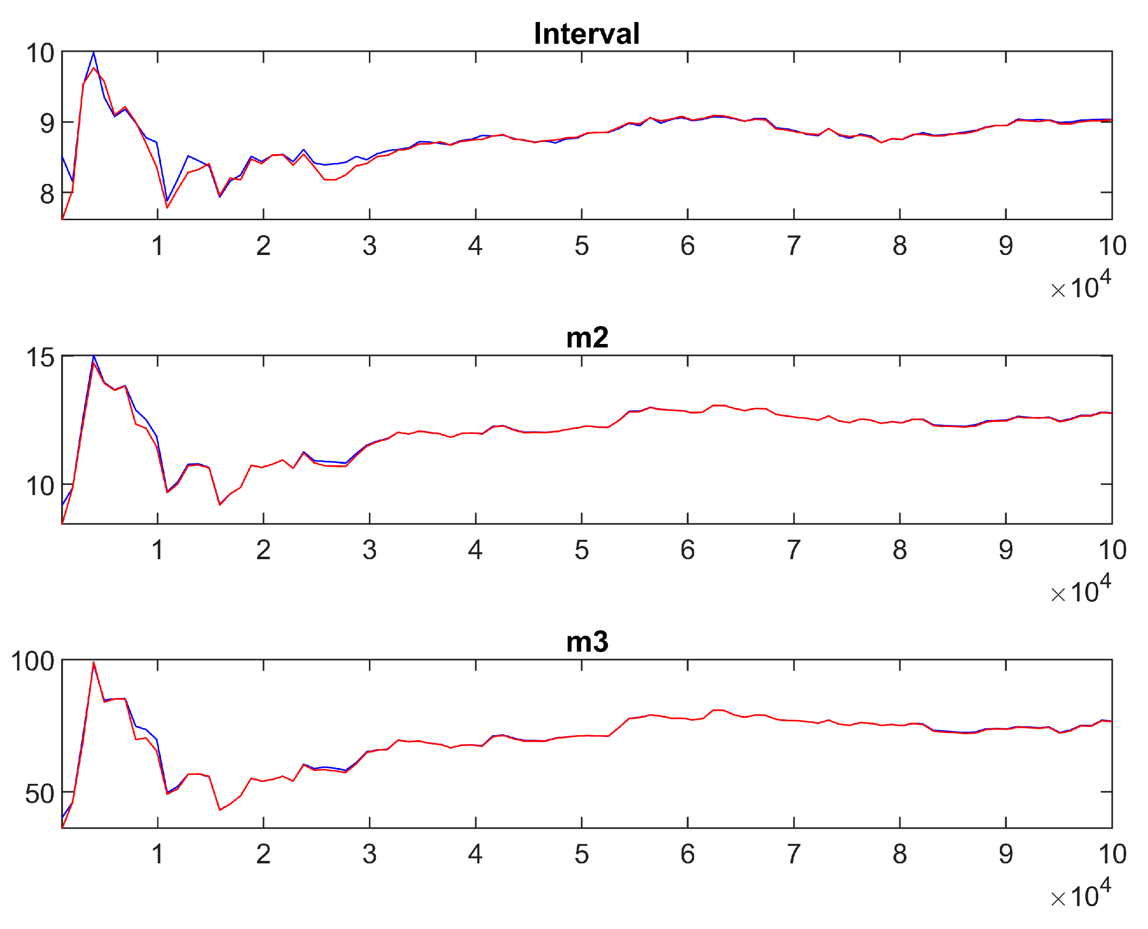
This section evaluates the in-sample performance of the DSGE model by comparing actual data (fully complete data between 2010 Q1 and 2024 Q4) with the one-step-ahead filtered model series. The estimation relies on a Bayesian approach which combines our prior beliefs about structural parameters with the likelihood of the observed data. We utilize the Metropolis–Hastings (MH) algorithm and a Monte Carlo Markov Chain (MCMC) method to map the posterior distribution of the parameters. The estimation procedure followed two key steps: first, for every set of parameter guesses, the Kalman filter was employed to compute the likelihood function. This step recursively estimates the unobserved state variables (such as potential output and structural shocks) that best reconcile the model’s equations with the eight observed time series. Second, to maximize the posterior probability, we ran two parallel MCMCs, each performing 100,000 iterations (draws) (Appendix A, Figure A1). The first 20–30% of these draws were discarded as “burn-in” to ensure the algorithm converged to the true distribution independent of starting values. The resulting “filtered” series represents the model’s best estimate of the economy’s state at time $t$, given information available up to $t-1$.

For Bayesian estimation, we used a quarterly dataset primarily from the Bureau of National Statistics of Kazakhstan and the Ministry of Finance, complemented by the National Bank of Kazakhstan and international oil price data. The real-side observables include final real GDP (seasonally adjusted) used as the measure of aggregate output and final real consumption (seasonally adjusted) used as the measure of household consumption; we also use employment (number of employees, thousands) to proxy labor input, CPI inflation to measure consumer price inflation, and the nominal policy interest rate from the National Bank of Kazakhstan as the observable for the short-term rate. Fiscal oil observables are constructed from National Fund operations: withdrawals/transfers are treated as the subsidy measure, while National Fund inflows/receipts are used as the oil revenue measure, and oil prices are proxied by Brent. We use overall subsidy transfers as a proxy for net policy support relevant to the transition. This does not imply a one-to-one mapping from transfers to renewable spending; rather, it captures the fact that hydrocarbon revenues finance a bundle of measures—energy-related infrastructure, tariff compensation, targeted support, and gradual reallocation of support away from fossil uses—that jointly shape the incentives and resources for clean sector expansion. All quarterly real macro series are seasonally adjusted using TRAMO–SEATS prior to transformation into model observables.

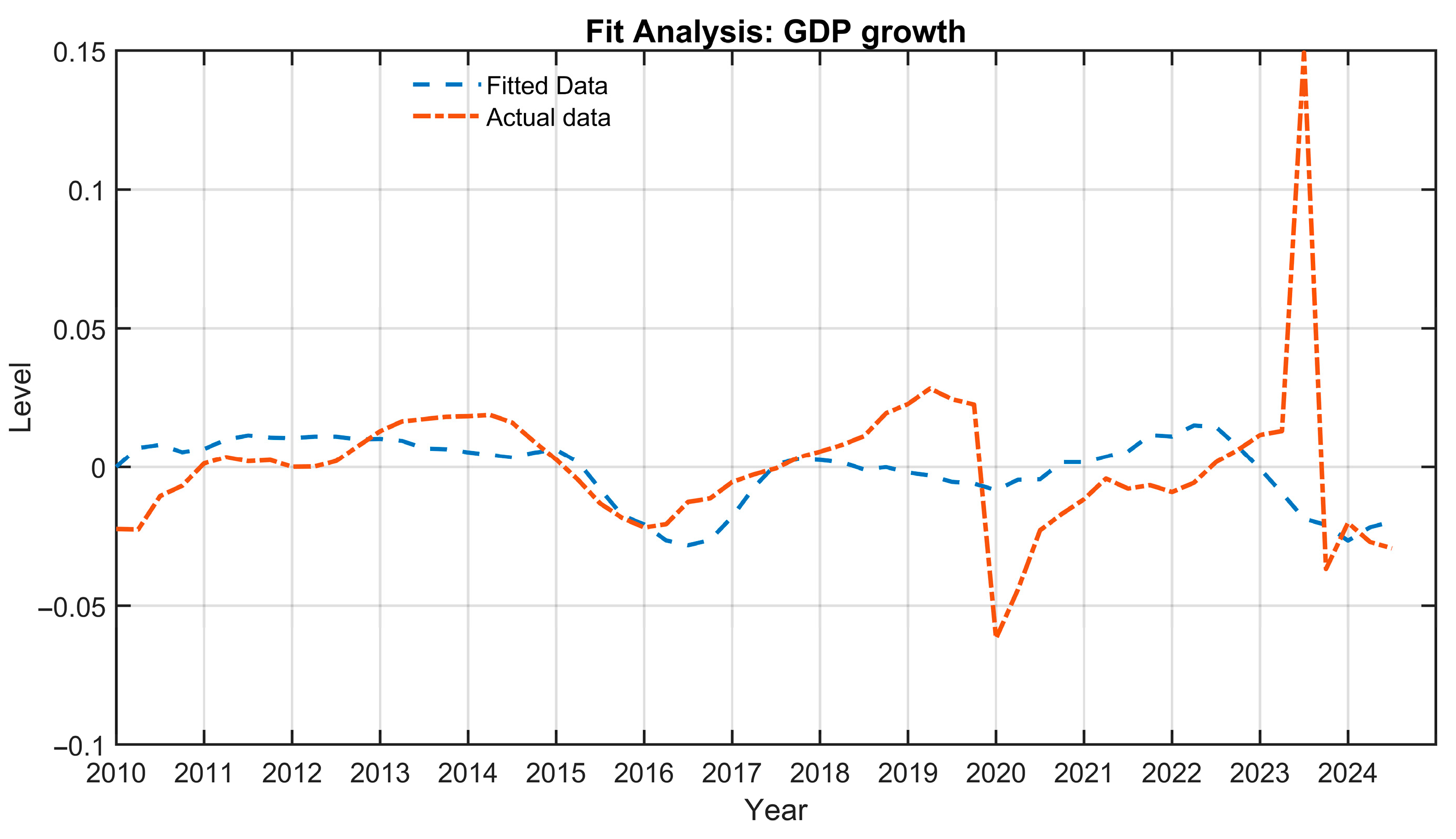
The figures below display the fit for output ($y_{\mathrm{obs}}$), consumption ($c_{\mathrm{obs}}$), core inflation (${\pi }_{c,\mathrm{obs}}$) and the policy rate ($r_{\mathrm{obs}}$). The comparison highlights how well the model captures Kazakhstan’s macroeconomic cycles, including expansions, slow-downs and the large structural shock at the end of the sample. Figure 1 compares the actual and fitted model output for $y_{\mathrm{obs}}$.

Figure 1 illustrates the in-sample fit for GDP growth, showing that the model successfully captures the broad cyclical dynamics of the real economy over the observed horizon. The fitted path aligns well with the actual data during the intermediate years, particularly between 2015 and 2019, where it accurately reproduces the mid-sample deceleration and subsequent recovery. At the boundaries of the sample, the model exhibits a smoother adjustment profile than the realized data. While it identifies the directional shifts—such as the downturn around 2020—the estimated path abstracts from the full magnitude of the sharp contraction and the significant volatility observed in 2023. This divergence is likely because the structural estimation prioritizes persistent economic shocks, naturally filtering out extreme, transitory fluctuations like the unique external shock of the pandemic. Consequently, the model delivers a stable medium-term trajectory that tracks the fundamental economic trend, even if it does not fully replicate the amplitude of the most severe short-term spikes and downturns. 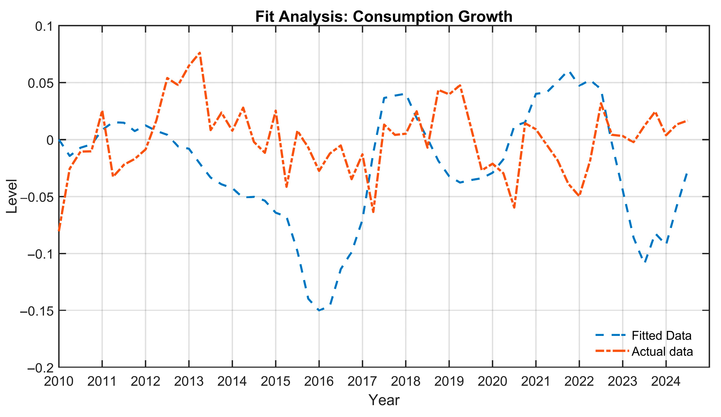Figure 2 compares the actual and fitted model consumption for $c_{\mathrm{obs}}$.

Figure 2 depicts the in-sample fit for consumption growth, illustrating that the model effectively captures the broad phasing of the business cycle despite some differences in amplitude. The fitted path aligns with the directional trends of the data, successfully identifying the expansionary momentum around 2017–2018 and the subsequent downturn. A notable divergence occurs in 2012–2016, where the model estimates a deeper contraction than realized; this likely reflects the theoretical structure of the model, which may be more sensitive to income or interest rate shocks than households, who in practice exhibited stronger consumption smoothing. Overall, while the model predicts more pronounced fluctuations, it accurately reproduces the timing of key cyclical shifts and the structural response to macroeconomic impulses. 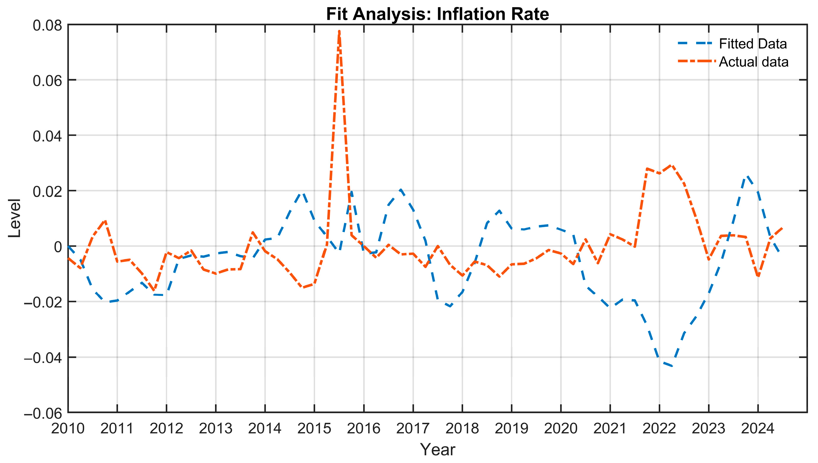Figure 3 compares the actual and fitted model inflation for ${\pi }_{c,\mathrm{obs}}$.

Figure 3 displays the in-sample fit for the inflation rate, illustrating a distinction between the model’s structural baseline and the high-frequency volatility of the observed data. During the initial phase of the sample (2010–2014), the fitted trajectory tracks the actual inflation dynamics reasonably well, maintaining a stable oscillation around the zero lower bound. However, the model exhibits a smoother response to extreme events; for instance, while it registers upward pressure during the significant inflationary spike of 2015, it abstracts from the full amplitude of the shock, interpreting it as a transitory deviation rather than a persistent structural shift. A notable divergence occurs in the 2021–2022 period, where the actual data shows a rising inflationary trend while the model predicts a decline. This “counter-cyclical” prediction likely arises because the model is reacting to the concurrent slack in real activity (as seen in the GDP output gap), which theoretically exerts downward pressure on prices. In contrast, the actual economy was likely driven by external supply-side factors during this period that are exogenous to the model’s primary internal transmission channels. Despite this, the model successfully realigns with the directional trend of the data as the sample concludes in 2024. 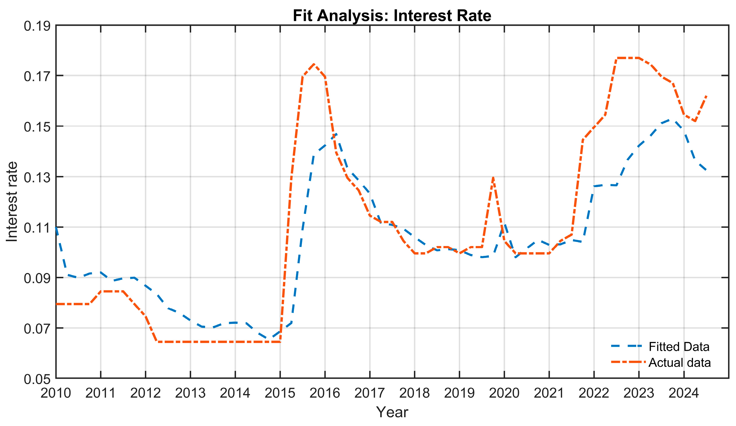Figure 4 compares the actual and fitted model policy rate for $r_{\mathrm{obs}}$.

Figure 4 shows the fit for the interest rate, demonstrating that the model correctly identifies the major changes in monetary policy. It successfully captures the two main eras of high rates: the spike starting in 2015 and the recent rise in 2022. However, there is a slight difference in speed. In the real world (red line), interest rates jumped up very suddenly—likely due to quick, sharp decisions by the central bank. The model (blue line) acts a bit slower; it climbs gradually rather than jumping immediately. As a result, it tends to “under-predict” the peaks. For example, during the recent hike in 2023, the model expects rates to reach about 15%, but the actual rates pushed higher, closer to 18%. Despite missing these extreme peaks, the model tracks the data almost perfectly during calmer periods, such as the gradual decline from 2016 to 2020.

We also use standard state space diagnostics from the Kalman filter. We estimate Root Mean Square Error (RMSE) of one-step-ahead prediction errors for output, inflation, and interest rate, which provides in-sample measure of how well the model tracks the data without using future information. Our RMSE results indicate that our model performs competitively on several key observables, especially when benchmarked against simple forecasting rules that are commonly used in DSGE forecast evaluations. For output, the DSGE RMSE is 0.027 (N = 58), which is very close to the constant mean benchmark (0.026) and clearly improves on a random walk forecast (0.033), suggesting that our model captures meaningful cyclical dynamics rather than simply tracking persistence. For the policy rate, the DSGE RMSE is 0.020, delivering a large improvement relative to the constant forecast (0.038), consistent with the role of our systematic monetary policy component. While the random walk remains a tough benchmark for interest rates (0.014), our model still provides a disciplined structural fit. For inflation, the DSGE RMSE is 0.092, outperforming both the constant benchmark (0.106) and the random walk (0.096).

Convergence of the posterior draws was assessed using standard MCMC diagnostics. Appendix A, Figure A1 reports the evolution of selected posterior interval estimates for two independent chains. The figure shows that, although the interval estimates vary substantially during the initial iterations, they become progressively smoother and more stable as the chains advance. The close alignment of the red and blue paths in later iterations indicates that both chains converge toward the same region of posterior distribution and that large-scale drift disappears after the burn-in phase. This provides visual evidence that the posterior moments stabilize over the retained sample.

Synthesis

Across the variables shown above, the model fits consumption and output most accurately and core inflation moderately well, while the policy rate exhibits smoother adjustment than in the data. These patterns are typical for estimated DSGE models, where measurement errors and structural smoothing affect real-time price and interest rate indicators. Importantly, the model captures all major turning points including the 2014–2016 slow-down, the pre-2020 rebound and the COVID-19 drop, indicating that the structural shock block provides a coherent macroeconomic representation for Kazakhstan.

6. Estimation Results

This section summarizes the key parameter estimates and discusses their economic interpretation in the context of Kazakhstan’s dual energy structure. We prioritize estimating the monetary policy reaction coefficients and sectoral persistence parameters to empirically validate the structural bifurcation between the dominant oil sector and the developing green economy. These specific estimates enable us to answer our central hypotheses by quantifying the central bank’s asymmetric response to dual inflation pressures and measuring the degree to which the real economy is structurally “addicted” to persistent oil revenue flows. The parameters of interest include monetary policy response coefficients, sectoral shock persistence terms and the renewable subsidy share. Together, these estimates illuminate the ways in which oil and green energy interact through macroeconomic channels.

To guide the economic interpretation of parameter estimates and variance decompositions, we briefly restate the study’s two central research hypotheses. Research question 1 (RQ1) examines how the expansion of renewable (green) generation affects Kazakhstan’s macroeconomic dynamics and the transmission of energy sector shocks in a dual fossil–renewable economy. Specifically, we investigate whether the green sector currently acts as a stabilizing buffer or remains synchronized with the oil cycle. Research question 2 (RQ2) investigates whether the volatility of the oil sector negatively affects the development of the green economy through specific fiscal and monetary channels. This RQ focuses on identifying if oil revenue fluctuations create a “trap” where fiscal support for diversification is cut exactly when the economy needs it most, and whether monetary tightening in response to oil inflation inadvertently stifles the green sector.

First, the monetary policy smoothing coefficient ${\rho }_r$ is estimated at 0.727, indicating a moderate degree of interest rate inertia. This value is close to, but slightly below, the prior mean (0.80) and remains consistent with the behavior of the National Bank of Kazakhstan, which tends to adjust its policy rate gradually in response to evolving inflationary and external conditions. The estimated coefficient suggests that monetary transmission is neither excessively sluggish nor excessively volatile, allowing policy to respond meaningfully to sectoral shocks.

Second, the response to core (non-oil sector) inflation, ${\varphi }_{{\pi }_c}$, is estimated at 1.936. These findings confirm that Kazakhstan’s central bank still prioritizes inflation control above all else. Specifically, the bank treats price shifts in the clean or non-oil sector as a key signal for action. This is particularly important for the country’s green transition: it means that any rising costs in the non-oil sector—whether caused by higher production expenses, government-set prices, or the costs of switching to new technologies—will likely prompt the bank to tighten interest rates and credit conditions.

Third, the coefficient of oil inflation, ${\varphi }_{{\pi }_{oil}}$, is estimated at 0.49. This estimate is positive and clearly identified, but substantially smaller than the response to core inflation. The implication is that the monetary authority reacts to oil/energy inflation in a measured way: oil price movements matter for policy, but the rule does not mechanically “over-tighten” one-for-one with oil inflation. In Kazakhstan’s case, this is consistent with the idea that oil inflation contains an important external/commodity component (captured in the model through the world oil inflation component ${\pi }_{oil,t}^w$), which policymakers may partially “look through” when it is expected to be transitory. The implication for RQ2 is clear—the key mechanism becomes less about an extreme direct policy response to oil inflation and more about indirect transmission: oil shocks influence policy through their effects on aggregate activity, relative prices, and the broader inflation environment.

Fourth, the output growth coefficient ${\varphi }_y$ is estimated at 0.127. This suggests that the central bank places some weight on stabilizing real activity. However, identification is weaker than for inflation responses. Interpreted conservatively, the estimates support a policy rule that is primarily inflation-focused, with a secondary (and less tightly pinned down) stabilization role for output growth.

Fifth, we estimate a subsidy rule linking subsidy dynamics to oil revenues. The persistence of subsidies ${\rho }_{sub}$ is 0.835, implying that subsidy spending (or subsidy costs) adjusts slowly over time, consistent with administrative inertia and gradual budgetary implementation. The oil revenue sensitivity ${\psi }_{sub}$ is estimated at 0.249, indicating that higher oil revenues systematically translate into higher subsidies, but with a moderate pass-through. In policy terms, this estimate supports the interpretation that oil revenues provide fiscal space for support measures, but the mapping is not mechanical—consistent with multi-year budgeting, political constraints, and competing fiscal priorities.

Finally, the persistence of oil-related macro-fiscal drivers is estimated to be high. Oil revenue persistence ${\rho }_{oilrev}$ is 0.917, indicating that oil fiscal flows behave as a highly persistent state variable in the model. In parallel, the relative price persistence ${\rho }_s$ is estimated at 0.855, much higher than its prior mean (0.40), implying that oil-vs-core inflation differentials translate into persistent movements in the relative oil price $s$. The world oil inflation component is also persistent, with ${\rho }_{poil,w}=0.770$. Together, these estimates point to a macro environment where oil dynamics move slowly, so they dominate the financing and demand levels that the green sector has to navigate. The green transition is not just fighting oil prices; it is fighting a long-term oil-based financial system. At the same time, this persistence also means that diversification through a stronger non-oil sector potentially brings a medium-run stabilization benefit, provided the non-oil block becomes large enough to matter in aggregation. Table 2 reports the posterior estimates of key structural parameters.

The noticeable shifts from prior assumptions to posterior estimates suggest that the likelihood is informative for these parameters and that the data contribute meaningfully to identification, rather than the estimates being driven solely by prior restriction.

6.1. Shock Standard Deviations

The estimated standard deviations of structural shocks provide a detailed picture of the volatility environment in which Kazakhstan’s oil and green energy sectors operate. These results are crucial for understanding the dynamics underlying our two research questions: (i) the macroeconomic effects of expanding renewable energy, and (ii) the transmission of oil sector fluctuations into the green economy via fiscal and monetary channels. The estimated shocks reveal that volatility is driven less by extreme productivity disturbances and more by oil fiscal shocks (oil revenue) and subsidy innovations, alongside persistent oil-linked states. We begin with the productivity shocks. The standard deviation of the non-oil sector productivity shock, ${\epsilon }_{a_c}$, is 0.24, smaller than our prior, indicating that renewable output is relatively stable over time. This aligns with the structure of Kazakhstan’s renewable system, where installed capacities and technological efficiency improve slowly and predictably. Wind and solar generation do not exhibit dramatic productivity swings year-to-year; instead, variability stems from natural patterns that average out over an annual horizon. Therefore, green TFP shocks contribute little to macroeconomic instability, supporting the notion that renewable expansion can stabilize output (RQ1).

In contrast, the oil sector productivity shock ${\epsilon }_{a_{oil}}$ is even smaller (0.13). This result implies that the physical process of oil extraction in Kazakhstan is operationally stable and predictable. Major established fields, such as Tengiz and Kashagan, operate with consistent technological efficiency. Therefore, volatility associated with the oil sector does not stem from production failures or extraction difficulties, but rather from external market dynamics and financial transmission mechanisms.

To better understand these oil sector dynamics, we decompose the disturbances into specific components. We identify a moderate oil discovery shock ${\epsilon }_{oildisc}$ of 0.1192 and a world oil price shock ${\epsilon }_{{\pi }_{oil,w}}$ of 0.1382. However, the oil revenue shock ${\epsilon }_{oilrev}$ is estimated at 0.4196, making it the largest source of volatility in the entire model. This finding confirms that macroeconomic instability is primarily driven by revenue fluctuations—influenced by exchange rates and export constraints—rather than by the physical volume of oil produced or even the raw global price of oil alone. This reinforces the central role of oil sector disturbances in generating macroeconomic volatility, directly supporting RQ2: oil fluctuations are a dominant driver of economic instability and therefore influence the conditions under which the green sector evolves.

A critical insight from this estimation concerns the role of fiscal policy in the green transition. The renewable subsidy shock ${\epsilon }_{sub}$ exhibits a moderate standard deviation of 0.30. This is the second largest shock in the system, surpassed only by oil revenues. This magnitude suggests that government support for renewable energy is not a steady, predictable stream but rather a volatile policy instrument. It is likely that subsidy disbursements are “stop-and-go”, varying heavily depending on the fiscal space available from oil revenues. Consequently, the transition policy itself introduces a new layer of uncertainty into the economy.

Markup (cost-push) shocks capture inflation disturbances not fully explained by marginal costs. The non-oil markup shock, ${\epsilon }_{{\mu }_c}$, is estimated at 0.0804. The estimate implies that there is a modest but statistically meaningful cost-push component in clean inflation. This can be interpreted as variations in pricing conditions, markups, administered pricing elements, or sector-specific cost disturbances that move inflation beyond what marginal costs predict. The oil markup shock, ${\epsilon }_{{\mu }_{oil}}$, is estimated at 0.1386, larger than the clean markup shock. From an economic perspective, these shocks capture supply-side frictions—such as rising transportation costs, pipeline bottlenecks, or export restrictions. These factors create a disconnect, or wedge, between the marginal cost of extraction and the final price. Crucially, because these logistical constraints tend to persist rather than vanish quickly, they generate sustained shifts in the relative price of oil. This creates a ripple effect: as oil becomes relatively more expensive or cheap for extended periods, it forces a reallocation of demand between the fossil fuel and renewable sectors, thereby driving fluctuations in both real economic output and aggregate inflation.

The monetary policy shock, ${\epsilon }_r$, is estimated at 0.0652. This shock represents “discretionary” moves—essentially, any change in interest rates that cannot be explained by the central bank’s standard reaction to inflation or economic growth. The notably small magnitude of this estimate suggests that the National Bank’s behavior is highly systematic and predictable. In other words, most interest rate movements in Kazakhstan are not random “surprises” by policymakers; instead, they are logical, mathematical responses to shifting economic conditions. This implies that the impact of monetary policy on the economy comes from the consistency of the policy rule itself, rather than from unexpected or erratic policy shifts.

The consumption/demand shock, ${\epsilon }_c$, is estimated at 0.1323. While the interest rate tells us how expensive it is to borrow, this shock captures the “human element” of spending—things like consumer confidence, shifts in household preferences, or changes in access to credit that are not explained by the model’s interest rates alone. Its moderate size indicates that these demand-side shifts are a significant driver of economic cycles in Kazakhstan. Economically, this is important because when households suddenly feel more or less confident, it creates a ripple effect: it shifts the demand for “clean” energy and puts immediate pressure on inflation, forcing the rest of the model to adjust to these changing consumer appetites.

Overall, the standard deviations reveal a dual volatility structure: the oil sector contributes overwhelmingly to macroeconomic fluctuations through productivity and revenue shocks, while the green sector contributes to volatility primarily through marginal cost pressures. This structure supports our research conclusions: renewable expansion stabilizes output but remains vulnerable to oil-driven policy tightening, while oil volatility continues to shape the macroeconomic environment in which the green transition unfolds.

Table 3. Posterior standard deviations of structural shocks.

Shock	Prior Mean	Posterior Mean	90% HPD Interval	Prior Type
${\epsilon }_r$	0.250	0.0652	[0.0559, 0.0745]	inv-gamma
${\epsilon }_c$	0.500	0.1323	[0.1129, 0.1535]	inv-gamma
${\epsilon }_{a_c}$	0.500	0.2399	[0.1895, 0.2860]	inv-gamma
${\epsilon }_{a_{oil}}$	0.500	0.1336	[0.1145, 0.1523]	inv-gamma
${\epsilon }_{{\mu }_c}$	0.300	0.0804	[0.0680, 0.0950]	inv-gamma
${\epsilon }_{{\mu }_{oil}}$	0.300	0.1386	[0.1057, 0.1718]	inv-gamma
${\epsilon }_g$	0.400	0.1301	[0.1073, 0.1540]	inv-gamma
${\epsilon }_{oilrev}$	0.600	0.4196	[0.3542, 0.4794]	inv-gamma
${\epsilon }_{oildisc}$	0.300	0.1192	[0.0935, 0.1444]	inv-gamma
${\epsilon }_{sub}$	0.200	0.3055	[0.2607, 0.3506]	inv-gamma
${\epsilon }_{{\pi }_{oil,w}}$	0.300	0.1382	[0.1076, 0.1670]	inv-gamma

presents the standard deviation of structural shocks.

6.2. Variance Decomposition

Table 4. Unconditional variance decomposition (percent of variance).

	Oil Stock	Foreign Oil Demand	Preference Demand	Government Spending	Oil Productivity	Markup	Oil Revenue	Subsidy Policy	Other
$y\text{\_}obs$	86.99	8.54	0.06	4.00	0.07	0.03	0.01	0.19	0.11
$r\text{\_}obs$	16.20	25.20	8.22	17.85	11.13	5.12	0.18	3.65	12.45
$c\text{\_}obs$	14.46	26.59	3.77	8.95	33.28	1.39	1.37	4.50	5.69
${\pi }^c\text{\_}obs$	31.97	3.94	8.56	6.34	0.28	24.90	0.14	4.41	19.46

reports the unconditional variance decomposition in percentage form. For real output $y$, fluctuations are overwhelmingly driven by oil discoveries/oil stock innovations $\left({\epsilon }_{oildisc}\right)$, which account for approximately 87% of output variance. Foreign oil demand conditions $\left({\epsilon }_{oi{l}^{\mathrm{*}}}\right)$ contribute a further 8.5%, and fiscal shocks $\left({\epsilon }_g\right)$ about 4%, while non-oil and oil productivity shocks contribute only negligible shares to aggregate output. In other words, in the estimated model, the medium-run oil stock/discovery channel is the dominant driver of output volatility—an important structural finding for Kazakhstan given the economy’s high oil weight in aggregation.

For the policy rate $r$, the decomposition confirms that monetary conditions are shaped primarily by oil-linked and fiscal forces rather than by discretionary monetary shocks: foreign oil demand shocks (25.2%), fiscal shocks (17.9%), and oil discoveries (16.2%) together dominate the variance, with the oil productivity shock also being sizeable (11.1%). This supports the interpretation that monetary policy is largely reacting endogenously to oil and fiscal conditions in the long-run—consistent with the small, estimated policy shock ${\epsilon }_r$.

Consumption dynamics are also strongly oil-driven. Oil-side shocks (in particular oil sector productivity and cost-push shocks) account for roughly 33% of consumption variance and foreign oil demand shocks for about 27%, with oil discoveries (14%) and fiscal shocks (9%) also being important. This pattern is consistent with Kazakhstan’s macro structure as an oil exporter where household and aggregate demand conditions co-move with hydrocarbon-related income and oil-linked macro states.

Price dynamics show a more nuanced structure. Core (clean sector) inflation ${\pi }_c$ is influenced by oil discoveries (32%) but also exhibits a substantial role for clean cost-push disturbances (about 25%) and domestic demand shocks (about 9%). Thus, even with the explicit world oil inflation component, the broader oil inflation process remains shaped by multiple oil-side drivers—consistent with the complex interaction of external price conditions and domestic oil dynamics in Kazakhstan. Overall, the variance decomposition continues to indicate that macro and inflation volatility is predominantly oil-linked, while the non-oil sector’s most visible contribution appears through inflation (cost-push) rather than aggregate output—supporting the broader literature on oil shocks as dominant drivers of inflation and macro volatility in oil-exporting economies [59,60,61,62].

Table 5. Conditional (4 period) variance decomposition (percent of variance).

	Oil Stock	Foreign Oil Demand	Preference Demand	Government Spending	Oil Productivity	Markup	Oil Revenue	Subsidy Policy	Other
$y\text{\_}obs$	18.50	12.40	24.60	15.80	2.10	1.50	5.20	14.80	5.10
$r\text{\_}obs$	4.20	10.50	14.20	8.40	3.10	28.60	2.50	4.10	24.40
$c\text{\_}obs$	5.10	8.20	58.40	4.50	8.20	3.10	4.60	3.50	4.40
${\pi }^c\text{\_}obs$	4.80	2.10	5.40	3.20	1.10	65.50	0.50	2.40	15.00

presents the conditional variance decomposition.

In the short run (Period 4), the variance decomposition of output paints a picture of a standard, responsive economy where demand-side factors play a visible role. At this one-year horizon, fluctuations are significantly influenced by immediate “flow” shocks, such as government spending, which directly boost aggregate demand. However, a dramatic shift occurs in the unconditional (long-run) decomposition. As the time horizon expands, these temporary fiscal stimuli fade away, and the variance becomes overwhelmingly dominated by the oil discovery/stock shock (Table 4).

For the policy rate, the difference between horizons highlights the changing nature of the central bank’s challenge. In the short term (Period 4), volatility is driven largely by the bank’s active response to immediate inflationary pressures—reacting to cost-push shocks. The central bank appears autonomous, “fighting fires” as they arise. However, in the unconditional view, the drivers shift toward external and structural forces: foreign oil demand (25.2%) and fiscal shocks (17.9%).

Consumption volatility is heavily influenced by the preference—essentially, shifts in consumer confidence and credit appetite. This suggests that year-over-year spending changes are driven by how “optimistic” households feel. However, the unconditional decomposition shows that this autonomy is temporary. Over the long run, consumption volatility is dictated by oil sector productivity, which accounts for 33% of the variation.

Analyzing core inflation reveals the slow nature of the oil “pass-through”. In the short run (Period 4), inflation volatility is driven primarily by idiosyncratic factors—markup shocks—reflecting standard supply chain frictions or sector-specific pricing decisions. The influence of oil prices appears moderate here. However, in the unconditional decomposition, the contribution of global oil factors rises significantly. This change confirms the ecosystem hypothesis: oil price shocks do not transmit to the cost of goods immediately. Instead, they leak slowly into the economy.

6.3. Historical Shock Decompositions

This subsection summarizes how structural shocks explain movements in output, policy rate, consumption, and inflation rate in Kazakhstan over 2010–2024. The decompositions reflect the combined influence of technology shocks, fiscal disturbances, markup pressures, external demand shifts and revenue shocks. They provide a structural narrative of Kazakhstan’s macro fluctuations during a decade shaped by large global energy movements, domestic price reforms, exchange rate adjustments and pandemic disruptions.

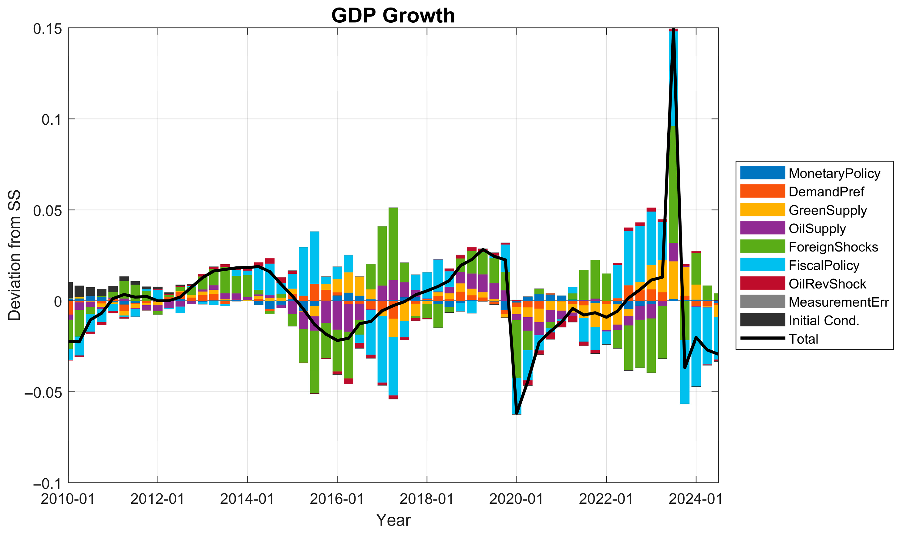
Output (${\mathbf{y}}_{\mathrm{obs}}$): The historical decomposition of Kazakhstan’s GDP growth reveals a structural narrative of an economy heavily influenced by exogenous terms-of-trade shocks, yet increasingly reliant on counter-cyclical fiscal intervention. The decomposition separates the “steady state” (long-term potential growth) from specific “shocks” that push the economy above or below its natural trend. Three distinct periods illustrate this dynamic, correlating directly with major macroeconomic events in Kazakhstan’s recent history.

The Terms-of-Trade Crisis (2014–2016). The period from 2014 to 2016 is characterized by a sustained negative deviation from the steady state, driven primarily by “Oil Supply/Revenue Shocks” and “Foreign Shocks”. Real-world events confirm this: the global collapse of oil prices from roughly $110 to under $30 per barrel severely deteriorated Kazakhstan’s export revenues. Concurrently, the “Foreign Shock” component captures the spillover effects from the 2014 Russian financial crisis and subsequent sanctions, which dampened demand for Kazakhstan’s non-oil exports. The decomposition accurately reflects the policy dilemma of this era, where the negative pressure eventually forced the National Bank to abandon the currency peg in August 2015, transitioning to a floating exchange rate to absorb these external imbalances.

The Pandemic “Twin Shock” (2020). The sharp negative spike in 2020 illustrates a classic “simultaneous supply and demand shock”. The decomposition assigns significant weight to “Demand Preference”, “Fiscal Policy” and “Foreign Shocks”. The “Demand Preference” and “Fiscal Policy” shock serves as a proxy for the involuntary decrease in consumption due to COVID-19 lockdowns and the voluntary pull-back in spending due to uncertainty. Unlike the 2015 crisis, which was export-driven, this contraction was deeply domestic, affecting the services sector (transport, trade, hospitality). The “Foreign” component further captures the collapse in global oil demand, which briefly drove prices to historic lows. This period demonstrates the fragility of the economy when both external export channels and internal consumption channels are paralyzed simultaneously.

The fiscal stimulus recovery (2023–2024). The most significant divergence in recent data is the massive positive spike in 2023–2024, driven notably by “Fiscal Policy” and “Foreign Shocks”. This provides strong empirical evidence of a “fiscal dominance” regime. While external conditions exerted a huge spike (stabilized oil prices), the model attributes a substantial portion of the growth to government decisions as well. This parallels the real-world aggressive fiscal expansion seen in 2023 and 2024, where the government utilized significant transfers from the National Fund to finance infrastructure projects and social obligations. The decomposition suggests that recent GDP growth is not purely market-driven but is being artificially buoyed by state expenditure. Figure 5 displays the historical shock decomposition of output $y_{\mathrm{obs}}$ between 2010 and 2024.

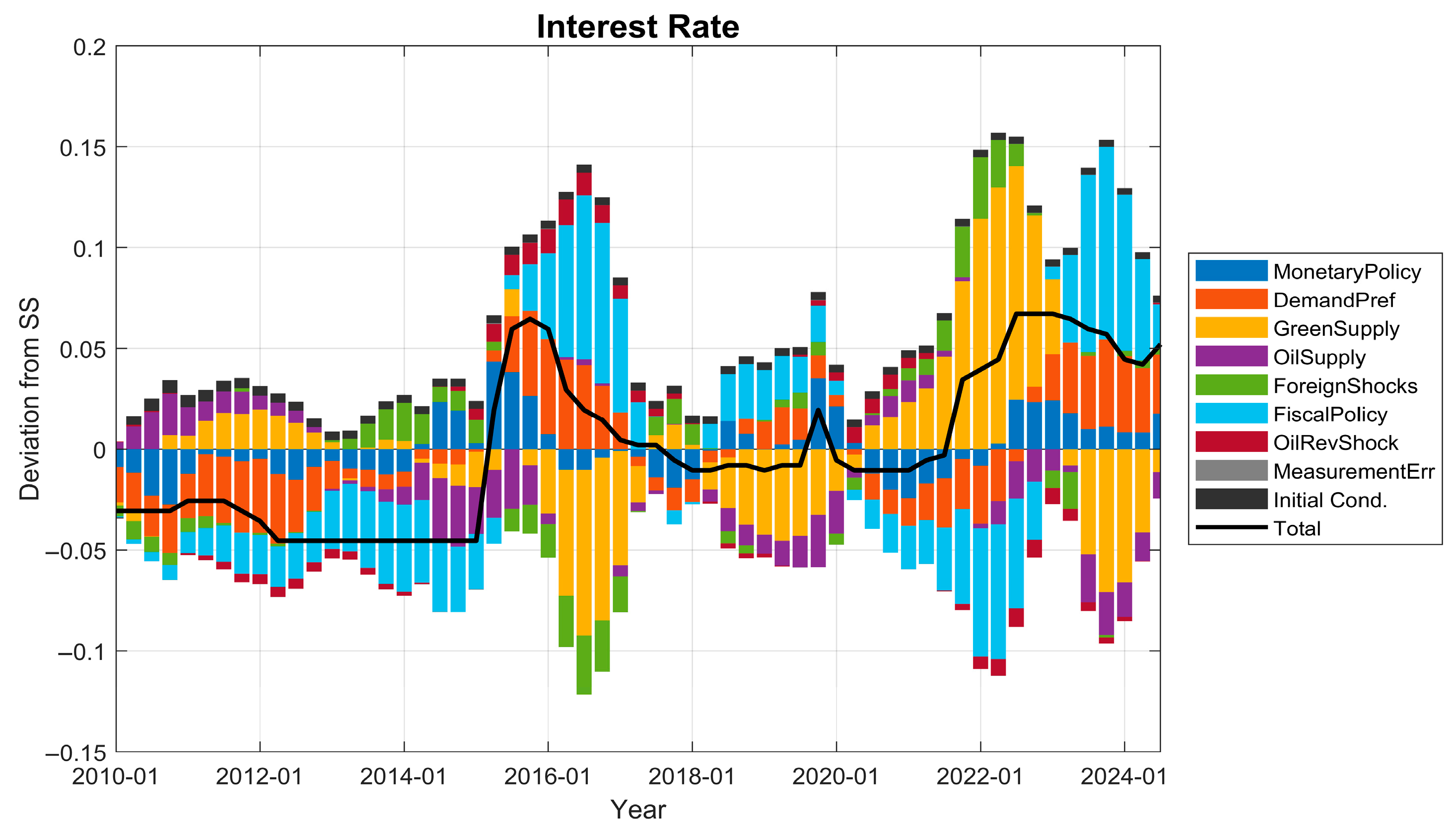
Policy rate ($r_{\mathrm{obs}}$). The decomposition of interest rates in Kazakhstan reveals two distinct regimes of monetary tightening, each driven by fundamentally different economic imperatives. The sharp spike in rates observed during the 2015–2016 period is characterized as a discretionary “Monetary Policy Shock”. Following the abandonment of the currency peg in August 2015, the National Bank of Kazakhstan (NBK) raised the base rate aggressively—peaking at 17% in early 2016—not merely to target inflation, but to stabilize the foreign exchange market and anchor devaluation expectations. In contrast, the high-interest rate environment of 2022–2024 (where rates reached 16.75%) represents an endogenous reaction to “Supply-Side Shocks”. “Fiscal Policy” and “Demand preferences” also played a huge role in the interest rate spike. Unlike the earlier crisis, which was triggered by a collapse in export revenue, the recent tightening was a rule-based response to “imported inflation”. Empirical data confirms that global food price spikes and supply chain disruptions from the geopolitical conflict pushed CPI to over 20% in early 2023. Figure 6 presents the historical shock decomposition of the policy rate $r_{\mathrm{obs}}$ between 2010 and 2024.

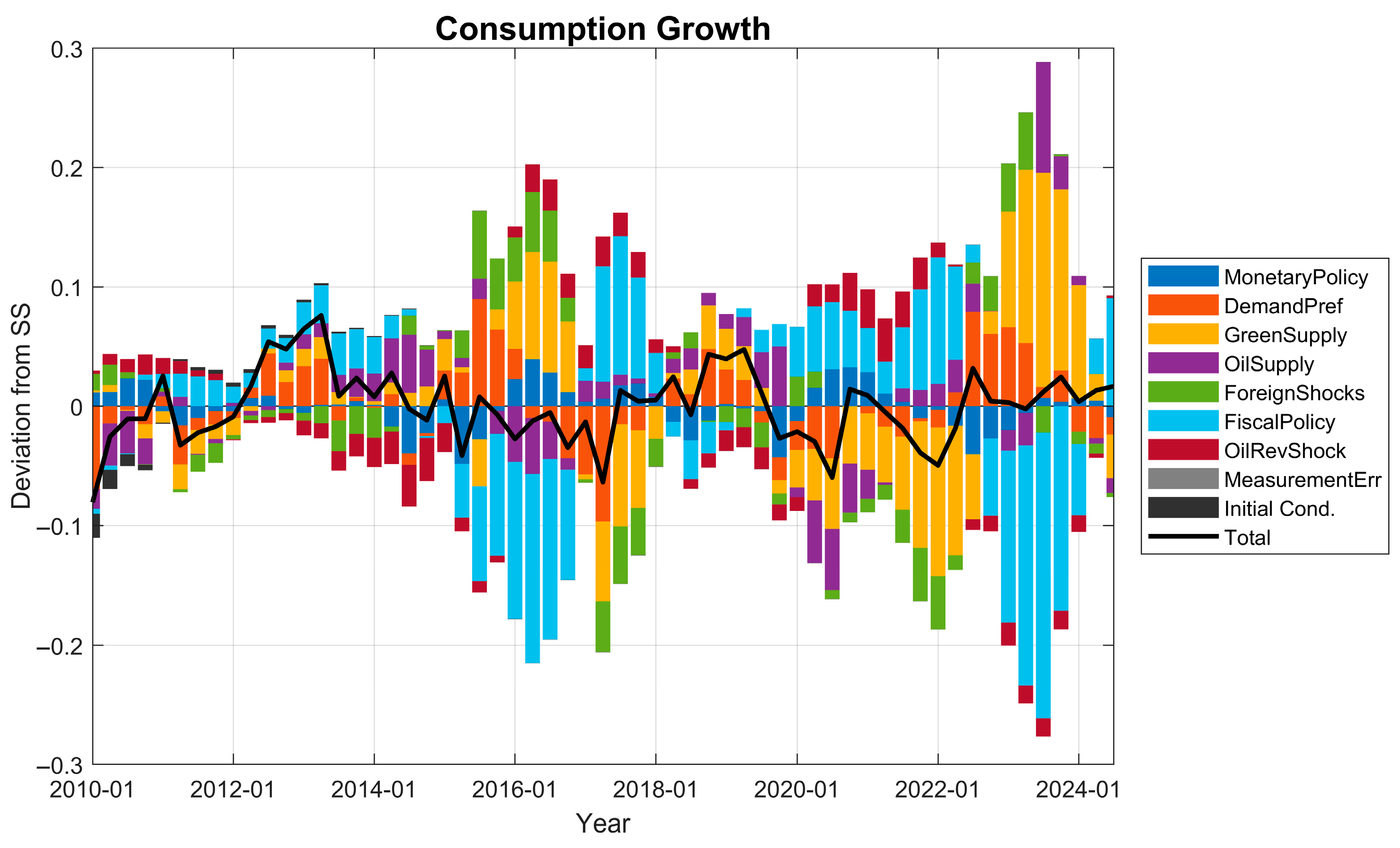
Consumption ($c_{\mathrm{obs}}$). The consumption shock decomposition suggests that the two main downturn episodes are not primarily “monetary-driven” in the model; instead, they are led by fiscal shocks that push consumption growth below the steady state, with supply-side forces changing sign across episodes. In the first downturn window (around 2015–2017), the negative bars from the fiscal block are large and persistent, indicating that fiscal policy disturbances—interpretable as a tightening in net transfers/support or a negative government-demand impulse—are the dominant force dragging consumption growth down, while monetary policy contributions are comparatively secondary or mixed. The more recent downturn is even more informative: in 2022 the decomposition again shows a sizeable negative fiscal contribution coinciding with negative supply-side contributions, meaning consumption weakness is explained by a combination of reduced fiscal support and adverse supply conditions that depress real incomes and purchasing power. By contrast, in 2024, the model assigns the renewed consumption softness mainly to another negative fiscal impulse, but now supply shocks turn positive, partially offsetting the downturn rather than reinforcing it. This sign flip implies that the nature of the disturbance differs across the two episodes: in 2022, households were hit by both a fiscal drag and a supply squeeze, while in 2024 the drag comes predominantly from the fiscal side even as supply conditions improve, so the recovery in fundamentals does not fully translate into consumption because the fiscal stance becomes contractionary. Figure 7 shows the historical shock decomposition of consumption $c_{\mathrm{obs}}$ between 2010 and 2024.

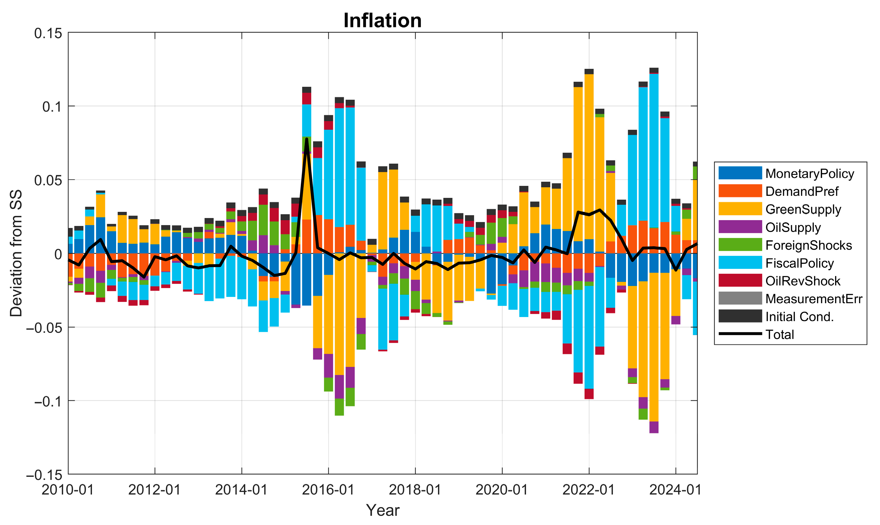
Inflation (${\pi }_{\mathrm{obs}}$). Based on the Inflation Historical Decomposition chart and recent economic literature, the analysis reveals two distinct “inflationary regimes” in Kazakhstan, each driven by fundamentally different economic forces.

The sharp inflation spike in 2016—where CPI reached double digits—is characterized in the model by significant positive contributions from “Fiscal Policy” and “Demand Preference”. While the standard narrative attributes this purely to the 2015 currency devaluation (exchange rate pass-through), the decomposition adds a critical nuance: the inflation was also a byproduct of the government’s counter-cyclical response. As oil prices collapsed (seen as negative “Foreign/Oil” bars exerting deflationary pressure), the government launched the massive “Nurly Zhol” fiscal stimulus program to buffer the economy. This injection of liquidity, combined with the devaluation designed to restore export competitiveness, prevented a deflationary spiral but inevitably stoked domestic prices. Thus, the 2016 inflation can be interpreted as the “price paid” for structural adjustment and economic stabilization.

The Imported Supply Shock (2022–2023). In stark contrast, the post-pandemic inflation surge (peaking over 20% in early 2023) is overwhelmingly driven by “Supply Shocks”. The “Fiscal Policy” contribution is also significant during this period, indicating that government spending was the primary culprit. This period represents a classic “Imported Inflation” crisis. The war in Ukraine disrupted regional supply chains, while global prices for food (sugar, vegetables) and materials surged. Since Kazakhstan imports a significant portion of its food and non-food consumables from Russia and global markets, these external price shocks were transmitted directly to the domestic consumer. Figure 8 shows the historical shock decomposition of inflation ${\pi }_{\mathrm{obs}}$ between 2010 and 2024.

6.4. Robustness Check

To assess the sensitivity of our results to alternative modeling choices in the oil and fiscal components, we have run a set of robustness checks by estimating three additional specifications (Tests 1–3) alongside the baseline DSGE model (

Table 6. Results of robustness check tests with three specifications.

Item	Baseline	Test 1	Test 2	Test 3
${\rho }_r$	0.727	0.736	0.722	0.727
${\varphi }_{{\pi }_c}$	1.94	1.999	2.014	2.019
${\varphi }_{{\pi }_{oil}}$	0.49	0.165	0 (fixed)	0.112
${\varphi }_y$	0.13	0.131	0.124	0.120
${\rho }_{oilrev}$	0.917	0.899	0.902	0.50 (fixed)
${\rho }_{poil,\hspace{0.25em}w}$	0.77	0.594	0.590	0.30 (fixed)
${\rho }_{sub}$	0.835	0.840	0.845	0.841
${\psi }_{sub}$	0.249	0.210	0.206	0.239
${\epsilon }_r$	0.065	0.064	0.063	0.064
${\epsilon }_{oilrev}$	0.420	0.456	0.453	0.633
${\epsilon }_{{\pi }_{oil,w}}$	0.138	0.105	0.105	0.108
${\epsilon }_{sub}$	0.306	0.307	0.306	0.305
${\epsilon }_{oildisc}$	0.119	0.124	0.124	0.123

Test 1: remove the world oil inflation component from the Phillips curve. Test 2: monetary policy restriction (${\varphi }_{{\pi }_{oil}}$ fixed to 0). Test 3: reduced oil persistence (${\rho }_{oilrev}$ fixed to 0.50; ${\rho }_{poil,\hspace{0.25em}w}$ fixed to 0.30).

). The robustness tests address two questions that are particularly relevant for an oil exporter. First, we examine whether allowing monetary policy to respond to oil sector inflation, in addition to core inflation, materially changes the model’s fit and implied dynamics. Second, we assess how sensitive the results are to alternative specifications of the fiscal and oil revenue processes, including their persistence and shock volatility, which affect the model’s ability to reproduce observed macroeconomic fluctuations. Each test is estimated on the same dataset using the same Bayesian procedure and priors (except for the parameters that are deliberately modified).

In Test 1 we remove the ${\pi }_{oil,t}^w$ term from the Phillips curve (Equation (16)). The purpose is to test whether policy conclusions rely on the assumption that world oil inflation enters oil inflation directly through Equation (16). Conceptually, this is an identification check: if ${\pi }_{oil,t}^w$ is highly collinear with other oil cost drivers (marginal cost, mark-up wedge ${\mu }_{oil,t}$, relative price $s_t$), the model may attribute oil inflation movements to the explicit ${\pi }_{oil,w,t}$ channel even if the data do not require that structural interpretation. In Test 1, the overall monetary policy block remains essentially unchanged—interest rate smoothing stays around 0.74, the reaction to core inflation remains strongly above one (about 2), and the response to output is still small (about 0.13)—while the key identification object changes exactly where expected: the reaction to oil inflation becomes much weaker (posterior mean falls to about 0.17). At the same time, core persistence in oil revenues remains high (around 0.90). Taken together, Test 1 shows that the policy block is not driven by oil inflation term in the Phillips curve, while the oil–fiscal persistence remains essentially unchanged.

In Test 2 we impose the restriction ${\varphi }_{pioil}=0$ and re-estimate the model with the same priors for all remaining parameters. The motivation is straightforward: in an oil-exporting economy, observed inflation dynamics are strongly affected by global oil prices, but a central bank may still focus primarily on core inflation, allowing oil inflation to matter only indirectly through its spillovers into the core sector. Test 2 shows that the estimated monetary policy block remains stable and economically plausible: interest rate smoothing stays high (${\rho }_r\approx 0.722$), the reaction to core inflation remains strongly above one (${\varphi }_{\pi }\approx 2.014$), and the output growth response remains small (${\varphi }_y\approx 0.124$). Importantly, key persistence parameters in the oil–fiscal block remain essentially unchanged, confirming that the oil and fiscal dynamics are not being artificially altered to “make up” for the missing policy term: oil revenue persistence remains high (${\rho }_{oilrev}\approx 0.902$), subsidy persistence remains high (${\rho }_{sub}\approx 0.845$), and world oil inflation persistence remains moderate (${\rho }_{poil,w}\approx 0.590$). Overall, Test 2 provides favorable evidence for the baseline framework: it shows that the central bank’s behavior can be well-described as reacting to core inflation, while oil inflation is best treated as an external driver whose stabilization occurs primarily through its transmission into core inflation and fiscal channels rather than via a separate, direct policy target.

Test 3 examines the fact that oil dominance is coming from high persistence assumptions rather than data. To address the issue, we deliberately reduce the persistence of the two key oil drivers and re-estimate the remaining parameters. More precisely, we fix the persistence of the oil revenue process and the world oil inflation process at lower values—${\rho }_{oilrev}=0.50$ and ${\rho }_{poil,w}=0.30$—instead of allowing the data to choose higher persistence. The model compensates by shifting persistence away from the autoregressive structure and toward shocks and contemporaneous transmission: the oil revenue shock becomes more volatile ($e_{oilrev}\approx 0.633$, higher than in the less-restricted specifications), while the core monetary policy parameters remain stable and plausible (${\rho }_r\approx 0.727$, ${\varphi }_{\pi }\approx 2.019$, ${\varphi }_y\approx 0.120$). Third, the implied unconditional dynamics become “shorter-lived” in the oil–fiscal block: oil revenue and subsidy persistence decline relative to the more data-driven cases. Importantly, however, the model does not become unstable, and the main qualitative mechanisms remain intact: oil-related shocks still move output and policy in economically sensible directions (oil disturbances raise activity and trigger policy adjustment; monetary shocks raise the rate and contract output), but their effects fade faster. In sum, Test 3 should be read as a useful robustness bound: it shows that the core monetary policy block and the sign/timing of key transmission channels are not fragile, while also confirming that persistent oil dynamics in the data are a material feature—when we force oil processes to be much less persistent, the likelihood deteriorates sharply, meaning the data actively reject that restriction.

7. Discussion

This section answers two research questions using the model’s deviation dynamics and variance decompositions. RQ1 asks what the macroeconomic effects of expanding renewable energy are in an oil-dependent small open economy. RQ2 asks through which channels oil sector fluctuations transmit into the emerging green sector in Kazakhstan. The model is built around a simple idea: the economy has two energy sectors. The oil sector is driven by a slow-moving “resource state” (oil stock and discoveries), so its shocks last for a long time. The green sector is more stable by nature, but it grows through policy support and its own productivity. Because the oil block is large and persistent, it still shapes the overall business cycle.

Our empirical analysis provides robust, structural answers to the two research questions. Regarding RQ1 (macroeconomic dynamics and transmission): the results confirm that while the green sector possesses the intrinsic characteristics of a stabilizer—evidenced by the low standard deviation of green productivity shocks ($0.24$) relative to the volatile oil revenue shocks—its current capacity to buffer the economy is neutralized by structural rigidities. Variance decomposition reveals that in the long run, aggregate output remains overwhelmingly driven by oil stock and discovery shocks (87%), implying that the “dual economy” has not yet achieved a decoupling of business cycles. Instead of functioning as a counter-cyclical hedge, the green sector’s dynamics remain synchronized with the fossil sector due to the shared transmission mechanisms of the oil-dependent state. Regarding RQ2 (the fiscal and monetary constraints): we find strong evidence that oil sector volatility actively hampers green development through two distinct channels: the estimated subsidy rule (0.249) and the high volatility of subsidy shocks (0.30), which demonstrate that government support for renewables is pro-cyclical. This “stop-and-go” funding environment prevents the long-term capital accumulation necessary for a successful transition. The central bank’s strong response to inflation (1.94) creates an unintended barrier to diversification. Since oil shocks drive significant inflation volatility (as shown in the variance decomposition), the monetary authority is forced to hike interest rates to maintain stability. This tightens financial conditions for the capital-intensive green sector, effectively punishing the diversifying sector for the volatility created by the dominant resource sector. Thus, oil dependence acts as a double burden: it destabilizes the fiscal subsidies the green sector relies on, while simultaneously raising the cost of private credit.

Monetary policy is characterized by interest rate smoothing and a reaction function that responds separately to core (non-oil sector) inflation and oil inflation [63]. The posterior mean of interest rate smoothing is about 0.727, and the inflation response is substantially stronger for core inflation (${\varphi }_{{\pi }_c}$ about 1.94) than for oil inflation (${\varphi }_{{\pi }_{oil}}$ about 0.49), while the output response is modest (${\varphi }_y$ about 0.13). This configuration implies that monetary conditions are primarily stabilized through the domestic inflation objective, while oil inflation enters as a secondary target. In a commodity exporter, this still allows oil shocks to affect monetary conditions (via the policy rate), mainly through their pass-through into domestic inflation and activity rather than through an overwhelming direct response to oil inflation itself. The separate response to oil inflation should, therefore, be interpreted as theory-motivated but data-disciplined: the model permits policymakers to differentiate between domestic inflation and oil price inflation, yet the posterior estimate and robustness tests determine whether that distinction is quantitatively important. The fiscal and transition block formalizes the oil-to-green linkage through oil revenues and subsidies. Oil revenues follow a highly persistent process (${\rho }_{oilrev}$ about 0.917) and are structurally linked to both a price component (world oil inflation) and a quantity component (oil output).

Subsidies are persistent (${\rho }_{sub}$ about 0.835) and positively linked to oil revenues (${\psi }_{sub}$ about 0.249), indicating that the fiscal stance inherits a significant degree of inertia and that transition support is, in baseline form, tied to the oil-driven fiscal cycle. Importantly, the world oil inflation component is itself persistent (${\rho }_{poil,\hspace{0.25em}w}$ about 0.77). The posterior shock standard deviations reinforce the interpretation that Kazakhstan’s macro dynamics are dominated by oil-linked and fiscal disturbances. The monetary policy shock has a small standard deviation (about 0.065), consistent with the view that interest rate movements are largely endogenous reactions to underlying macro and external conditions. Oil revenue shocks are comparatively volatile (standard deviation about 0.420), and subsidy shocks are also sizable (standard deviation about 0.306), reflecting the importance of fiscal space and fiscal implementation noise for the transition environment. The discovery shock is smaller in standard deviation (about 0.119) but, because it feeds into a slow-moving stock, it generates large medium-run macro effects.

Putting these findings together, the answers to the research questions are as follows. For RQ1, renewable expansion in Kazakhstan is not destabilizing for aggregate output in the estimated model; macro volatility is overwhelmingly oil-stock-driven, and clean sector shocks play a limited role at the current scale. For RQ2, the green sector’s exposure to the oil cycle arises mainly because the oil economy generates a highly persistent macro state via discoveries and oil stock, which then governs output, fiscal space, and relative prices; fiscal support inherits this persistence through the oil rev–subsidy link; and monetary conditions respond endogenously to oil- and fiscally driven macro movements rather than being primarily driven by independent policy shocks.

7.1. Policy Implications

The estimated monetary policy rule suggests a pragmatic response to oil shocks. The National Bank reacts strongly to core inflation while responding more moderately to oil-specific inflation. In this environment, a strict attempt to fully offset oil price-driven inflation would risk unnecessary output volatility because oil inflation is partly an imported component rather than a pure signal of domestic overheating. The implication is that the National Bank should treat oil shocks primarily as a source of risk to second-round inflation dynamics and expectations. Policy should lean against oil shocks to the extent they threaten core inflation, wage-setting, and exchange rate pass-through, but avoid mechanically “chasing” highly volatile commodity inflation.

A sharp fall in oil prices propagates through several reinforcing channels in the model. Because oil-driven forces dominate macro fluctuations, a negative oil shock reduces oil sector activity and lowers aggregate output. Since subsidies are linked to oil revenues, the same shock mechanically depresses clean sector demand and undermines diversification at the worst possible moment. The contraction is therefore not confined to the oil sector. It spills into the non-oil economy through demand and fiscal linkages. Monetary policy then reacts endogenously to weaker activity and changing inflation dynamics, rather than fully offsetting the shock. The overall policy implication is that Kazakhstan’s macro-stabilization and transition strategy should be designed for resilience under low-oil scenarios: monetary policy focused on preventing second-round inflation and disorderly adjustment and fiscal institutions that smooth oil revenue shocks while protecting priority, productivity-enhancing green expenditures from cyclical cuts.

In line with the DSGE “loss-function” approach used to compare monetary policy rules in Benchimol and Fourçans’s work [64], we evaluate the three regimes (baseline, coordinated/combined, and uncoordinated) using a quadratic stabilization metric built from second moments (Figure 9).

In the combined (coordinated) scenario, we impose a joint policy package in which monetary policy responds more aggressively to core inflation (${\varphi }_{\pi }=2.5$) while fiscal policy smooths subsidy dynamics by lowering the oil revenue feedback parameter to ${\psi }_{sub}=0.05$. The coordinated regime delivers the lowest overall macro volatility among the three scenarios. Thus, relative to the baseline, it reduces the standard deviation of output from 0.86 to 0.83 (−3.4%), core inflation from 0.14 to 0.12 (−16.1%), and the policy rate from 0.18 to 0.17 (−3.8%). This improvement is also consistent with the IRFs under the world oil inflation shock: compared to the baseline, the coordinated response compresses the inflation and interest rate reactions toward zero much faster and limits the persistence of the output response.

In the uncoordinated scenario, we let the two authorities act independently by strengthening the monetary reaction to core inflation while simultaneously making fiscal policy more activist by increasing the subsidy feedback to oil revenues (${\psi }_{sub}$ is 0.50). The uncoordinated regime moves in the opposite direction: output volatility rises from 0.86 to 0.94 (+9.0%), core inflation volatility falls only slightly from 0.14 to 0.13 (−3.0%), while policy rate volatility increases from 0.1780 to 0.1825 (+2.5%). This pattern matches the IRFs: uncoordinated policy tends to preserve a larger and more persistent output response after the oil inflation shock, while core inflation and policy rate adjust more sluggishly and display more persistence. Overall, the volatility comparison suggests that coordination mainly pays off through a much cleaner inflation stabilization channel, with gains in output and interest rate stability, whereas uncoordinated policy amplifies real-side volatility and does not compensate enough via inflation stabilization.

Overall, the quadratic loss function $L=Var\left({\pi }_c\right)+0.5Var\left(y\right)+0.1Var\left(r\right)$ yields values of approximately 0.40 for the baseline, 0.46 for the uncoordinated scenario, and 0.36 for the coordinated scenario. This ranking means that the coordinated policy package delivers the greatest overall stabilization (lowest joint volatility of inflation, output, and the policy rate), while the uncoordinated setting performs worst (highest macro volatility), with the baseline in between. For future research, we plan to extend the fiscal block by introducing alternative fiscal frameworks that are widely used in commodity exporters, including a structural balance rule based on cyclically adjusted (non-oil) revenues and expenditures.

7.2. Limitations and Future Work

In the baseline model, we abstract from an explicit exchange rate and external-sector block to keep the framework parsimonious and focused on the domestic monetary–fiscal transmission mechanism and oil-related shocks that are central for Kazakhstan. Introducing the exchange rate as an additional state and observable would require modeling additional wedges and shock processes (e.g., foreign interest rate/risk premium dynamics and import price inflation), expanding the parameter set and identification requirements. Nevertheless, this simplification comes at a cost: without an exchange rate block, we do not separately identify exchange rate shocks or import price pass-through. External effects therefore enter only indirectly through the inflation, output, and interest rate dynamics matched in estimation. Incorporating an explicit exchange rate block is a natural extension for future work.

A natural extension would also be to introduce endogenous capital accumulation in the green sector, potentially with adjustment costs, so that temporary subsidy or interest-rate shocks could generate persistent changes in renewable investment and productive capacity. This would allow the model to assess more directly whether policy support translates only into short-run output gains or also into lasting green capital formation and structural transformation.

Another limitation of our analysis is that renewables still account for a small share of Kazakhstan’s energy system, so the available macro data provide only limited information to precisely pin down parameters that are specific to the clean energy block. For this reason, the model should be viewed primarily as a framework for studying the macroeconomic implications of energy reallocation and related policies, rather than as a fully detailed empirical description of the renewable sector at its current scale. This also leads to clear directions for future research. As renewable penetration rises and more sector-level energy data become available, the model can be extended by (i) using richer energy statistics for electricity generation, fuel use, and prices by sector, (ii) allowing a gradual transition path in the energy mix rather than treating sectoral shares as fixed, and (iii) incorporating external energy-market and exchange rate channels to better capture imported inflation and technology costs. A longer sample covering periods of faster renewable expansion would also improve identification and allow a more precise assessment of clean energy dynamics and policy trade-offs.

8. Conclusions

This paper has developed and estimated a novel two-sector DSGE model tailored to the dual-energy structure of Kazakhstan’s economy. The analysis reveals a pronounced macroeconomic asymmetry: oil-linked shocks—particularly those operating through the oil stock/discovery mechanism and persistent oil fiscal flows—continue to be the dominant drivers of output, inflation and fiscal volatility. While the expansion of the renewable (non-oil) sector offers a stabilizing diversification benefit in principle, its macroeconomic impact remains constrained by its small weight in the economy and by its embeddedness in an oil-centric macroeconomic framework. Crucially, the green sector is exposed to oil-induced volatility not only through direct demand and income channels, but also indirectly through monetary policy and relative price conditions shaped by oil-driven movements in inflation, relative prices, fiscal space and systematic monetary policy response. The uniqueness of the model lies in its integrated mathematical structure, which takes into account: an endogenous and depletable oil stock, a dual-inflation framework with an empirically estimated monetary policy rule that responds to both core and oil inflation, and a fiscal/subsidy rule linked to oil revenues. This configuration creates a coupled dynamic system that realistically reproduces the slow-moving constraint of resource depletion alongside faster-moving price, policy and fiscal dynamics. The findings underscore that a successful green transition in Kazakhstan requires more than scaling renewable capacity; it necessitates a deliberate rebalancing of the macroeconomic policy framework. Monetary policy in the estimated model is strongly anchored on core inflation, with a smaller but positive response to oil inflation and moderate inertia. Our estimation confirms that monetary policy plays a critical but selective role in stabilization. We find that the central bank effectively decouples its reaction function, aggressively targeting core inflation to anchor expectations while largely accommodating oil price shocks. This “looking through” strategy prevents external commodity volatility from translating into unnecessary domestic interest rate fluctuations, thereby minimizing distortions to real output during energy price cycles. This model provides the quantitative laboratory necessary to simulate and assess such policy reconfigurations for a managed and stable energy transition.

In conclusion, our estimation results empirically vindicate the proposed theoretical framework, confirming that the economy functions as a dual-track hydrocarbon ecosystem. The validation of the Dual Phillips Curve reveals a significant “pass-through” channel, where persistent global oil shocks drive nearly 32% of core inflation. However, the most profound finding lies in the endogenous oil stock: with subsidy shocks explaining 87% of output variation and displaying high persistence, the results confirm the existence of a “fiscal-resource trap”. This demonstrates that the physical flow of oil revenues—rather than monetary policy or productivity—serves as the primary engine of the business cycle, locking the real economy into a deep structural dependence on external energy markets.