Type B (p, q)-Stirling Numbers via Signed Restricted Growth Functions and Rook Theory

Abstract

Stirling numbers are among the most classical objects in enumerative combinatorics, counting set partitions and permutations. In this paper, we study their $(p,q)$-analogues in type B from a rook-theoretic point of view. We introduce a type B Ferrers board and establish a bijection between signed restricted growth functions and type B rook placements. In addition, we defined the weighted statistics ${\mathrm{levLB}}_B\left(w\right)$ and ${\mathrm{levLS}}_{\mathrm{B}}\left(\mathrm{w}\right)$ over the set of signed restricted growth functions. The associated statistics yield a weighted enumeration that recovers the $(p,q)$-Stirling polynomials of type B, their recurrence relations and generating functions. We then introduce type B Laguerre boards and prove that their rook numbers coincide with the Lah numbers of type B.

1. Introduction

Stirling numbers of the second kind count set partitions (see [1]). It is well known that set partitions are in bijection with restricted growth functions (RGFs) (see [2]). Stirling numbers of the second kind also count the number of rook placements over staircase Ferrers board (see [3]). Type B analogues of set partitions were first introduced by Reiner [4] and later studied extensively by Sagan and Swanson [5]. These numbers count signed set partitions arising from Coxeter groups of type B. Along with these, Bagno, Biagioli, and Garber [6] obtained several identities for Stirling numbers of the second kind of types B and D. Wachs and White [7] showed that the q-Stirling numbers of the second kind arise as generating functions relating various statistics on set partitions. They also introduced $(p,q)$-Stirling numbers describing the joint distribution of left-bigger and left-smaller statistics. In addition, they provided bijections between restricted growth functions and rook placements on staircase Ferrers boards. However, to the best of our knowledge, a direct rook-theoretic interpretation of the $(p,q)$-Stirling numbers of type B has not previously been developed.

For type B set partitions, Acharyya [8] defined signed restricted growth functions (SRGF) and proved that they are in bijection with signed set partitions. Although SRGFs give a combinatorial description of type B set partitions, Acharyya [8] asked whether there exists an analogue of the $(p,q)$-Stirling numbers of the second kind for type B set partitions, together with a way to obtain generating functions for the corresponding joint distributions of statistics over signed restricted growth functions and type B rook placements. Briggs and Remmel [9] introduced m-rook placements on m-Ferrers boards and defined $(p,q)$-analogues of m-rook and m-hit numbers. Their work relates rook placements to signed permutations in the wreath product $C_m\wr S_n$ and studies some permutation statistics. However, their work does not provide a combinatorial model for $(p,q)$-Stirling numbers of type B defined via signed restricted growth functions. In this paper, we construct a type B Ferrers board associated with signed restricted growth functions and define statistics whose generating functions produce the $(p,q)$-Stirling numbers of type B.

In classical rook theory, Ferrers and Laguerre boards provide natural combinatorial models for Stirling and Lah numbers (see [10,11,12]). In particular, the Lah numbers describe the change of basis between rising and falling factorials. Such polynomial sequences and their generating functions also appear in operator-based approximation theory (see [13,14]). Lah numbers of type B play an important role in expressing rising factorials of type B in terms of falling factorials of type B (see [15]). The study of $(p,q)$-analogues of Lah-type numbers, such as the $(p,q)$-Whitney–Lah numbers introduced by Ramírez and Shattuck [16], suggests a natural direction for defining a $(p,q)$-analogue for the Lah numbers of type B.

Sagan [17] introduced a major index statistic on set partitions and proved that its generating function yields the q-Stirling numbers of the second kind. He also described this statistic through restricted growth functions and rook placements.

In this paper, we give a rook-theoretic construction for a $(p,q)$-analogue of the Stirling numbers of type B, motivated by the work of Sagan [17] as well as Wachs and White [7]. We first define a type B Ferrers board, whose column heights are determined by the signed restricted growth condition. We then show that rook placements on this board correspond bijectively to signed restricted growth functions. Under this correspondence, the level-weighted statistics on SRGF coincide with the deletion statistics defined on the board. This provides a rook model for the $(p,q)$-Stirling polynomials of type B. In particular, we obtain explicit recurrence relations and closed product formulas for their ordinary generating functions. We next consider a Laguerre board of type B and study rook placements on it. By introducing anchored placements, we obtain a rook-theoretic interpretation of the Lah numbers of type B.

The structure of the paper is as follows. Section 2 provides background on signed set partitions and signed restricted growth functions. In Section 3, we introduce the Ferrers board of type B and establish a bijection between SRGF and rook placement on Ferrers board of type B. After that, we develop the level-weighted statistics on SRGF and recurrence relations for $(p,q)$-Stirling polynomials of type B. Finally, we define the type B Laguerre board and show how it relates to Lah numbers of type B. We end with a section of open problems.

2. Preliminaries

We begin by introducing some basic definitions and notation that will be used throughout the paper. Let $\left[n\right]:=\{1,2,\dots ,n\}$, $\langle n\rangle :=\{-n,\dots ,-1,0,1,\dots ,n\}$ and let ${\langle n\rangle }^{\prime }:=\langle n\rangle \setminus \left\{0\right\}$. For $j\in \left[n\right]$, we denote the negative integer $-j$ by $\overline{j}$, and for a signed integer $x\in \langle n\rangle$, its absolute value is denoted by $\left|x\right|$.

Recall that set partitions of $\left[n\right]$ into k nonempty subsets, called blocks, are enumerated by the Stirling numbers of the second kind $S(n,k)$ (see [1]). A partition $\sigma =B_1|\cdots |B_k$ of $\left[n\right]$ is said to be in standard form if

$$min{B}_1<\cdots <min{B}_k.$$

Since $min{B}_1=1$, we will always assume that set partitions are written in standard form. We denote by ${\Pi }_n$ the set of all partitions of $\left[n\right]$ and by ${\Pi }_{n,k}$ the set of partitions of $\left[n\right]$ with exactly k blocks. Clearly, $|{\Pi }_{n,k}|=S(n,k)$.

The Stirling numbers of the second kind satisfy the recurrence

$$S(n,k)=S(n-1,k-1)+kS(n-1,k),$$

with initial condition $S(0,k)={\delta }_{0,k}$.

Signed set partitions of $\langle n\rangle$ and the corresponding Stirling numbers of the second kind of type B, denoted $S_B(n,k)$, were first defined by Reiner [4]. These numbers count signed set partitions with k paired blocks and satisfy the recurrence

$$S_B(n,k)=S_B(n-1,k-1)+(2k+1)S_B(n-1,k),$$

with initial condition $S_B(0,k)={\delta }_{0,k}$.

The q-analogue of the Stirling numbers of the second kind was introduced by Sagan [17]. A q-analogue of the type B Stirling numbers of the second kind was introduced by Sagan and Swanson [5]. The type B q-Stirling numbers, denoted $S_B[n,k]$, are defined recursively by

$$S_B[n,k]=S_B[n-1,k-1]+{[2k+1]}_q{S}_B[n-1,k],$$

with initial condition $S_B[0,k]={\delta }_{0,k}$, where

$${\left[m\right]}_q:=1+q+\cdots +q^{m-1}$$

denotes the q-integer.

We now recall some basic notions from classical rook theory that will be used throughout the paper. A board is a finite collection of unit squares arranged in rows and columns. A rook placement on a board B is a selection of squares such that no two chosen squares lie in the same row or the same column; equivalently, it is a placement of non-attacking rooks. For $k\ge 0$, a k-rook placement consists of exactly k rooks, and $r_k\left(B\right)$ denotes the number of such placements. The quantity $r_k\left(B\right)$ is called the k-th rook number of B (see [1]). In later sections, we consider signed boards with a modified notion of rook placement, in which the non-attacking condition is adapted to the type B setting and repeated signed row labels are permitted.

Closely related to rook-theoretic constructions are the classical Lah numbers. The (unsigned) Lah numbers $L(n,k)$ count the number of ways to partition an n-element set into k nonempty linearly ordered blocks (see [11]). Equivalently, $L(n,k)$ counts the number of ways to decompose an n-element set into k lists. These numbers were originally introduced by Lah in 1954 [11] and admit the explicit formula

$$L(n,k)=\left({\displaystyle \genfrac{}{}{0pt}{}{n-1}{k-1}}\right){\displaystyle \frac{n!}{k!}},1\le k\le n.$$

Ferrers boards play a central role in classical rook theory (see [10]). A Ferrers board is a board whose column heights form a weakly increasing sequence $b_1\le b_2\le \cdots \le b_n$. If B is a Ferrers board with column heights $b_1\le b_2\le \cdots \le b_n$, then a theorem of Goldman, Joichi, and White [10] gives the factorisation

$$\prod _{i=1}^n\left(x+b_i-(i-1)\right)=\sum _{k=0}^n{r}_{n-k}\left(B\right){\left(x\right)}_k$$

(1)

where ${\left(x\right)}_k:=x(x-1)\cdots (x-k+1)$ denotes the falling factorial.

As an illustration of the Goldman–Joichi–White product formula, consider the Ferrers board $B=B(1,4,7,\dots ,3n-2),$ whose column heights are given by $b_i=3i-2$ for $1\le i\le n$. Applying the product formula yields

$$\prod _{i=1}^n\left(x+b_i-(i-1)\right)=\prod _{i=1}^n(x+2i-1)=\sum _{k=0}^n{r}_{n-k}\left(B\right){\left(x\right)}_k.$$

Hence, we get

$${\left[x\right]}_B^n=\sum _{k=0}^n{r}_{n-k}\left(B\right){\left(x\right)}_k$$

(2)

where ${\left[x\right]}_B^n:=(x+1)(x+3)\cdots (x+2n-1)$ is the rising factorial of type B appearing in [5]. In [6], the falling factorial of type B is defined as ${\left(x\right)}_k^B:=(x-1)(x-3)(x-5)\cdots (x-2k+1)$.

Equivalently, Equation (2) shows that the coefficients $r_{n-k}\left(B\right)$ are the change-of-basis coefficients from the falling factorial basis ${\left\{{\left(x\right)}_k\right\}}_{k\ge 0}$ to the type B rising factorial basis ${\left\{{\left[x\right]}_B^n\right\}}_{n\ge 0}$. Polynomial sequences and their generating functions also appear in operator-based approximation theory (see [13,14]).

Another classical example in rook theory is the staircase Ferrers board $J_{n,1}=B(0,1,2,\dots ,n-1)$. It is a classical result, due to Kaplansky and Riordan [3], that the rook numbers of $J_{n,1}$ are expressed in terms of the Stirling numbers of the second kind. More precisely,

$$r_{n-k}\left(J_{n,1}\right)=S(n,k),0\le k\le n,$$

where $S(n,k)$ denotes the Stirling number of the second kind.

A particularly important role in the context of Lah numbers is played by the so-called Laguerre board, which may be viewed as a special case within the classical rook-theoretic framework. For $n\ge 1$, let ${\mathcal{L}}_n=B(n-1,n-1,\dots ,n-1)$ denote the Laguerre board consisting of n columns, each of height $n-1$. From the product formula in Equation (1), it follows that the rising factorial ${\left[x\right]}^n:=x(x+1)\cdots (x+n-1)$ has the rook expansion

$${\left[x\right]}^n=\sum _{k=0}^n{r}_{n-k}\left({\mathcal{L}}_n\right){\left(x\right)}_k$$

(3)

where $r_{n-k}\left({\mathcal{L}}_n\right)$ denotes the number of placements of $n-k$ non-attacking rooks on ${\mathcal{L}}_n$. Moreover, it is well known from [12] that the rising factorial can also be expressed as

$${\left[x\right]}^n=\sum _{k=0}^{n}L(n,k){\left(x\right)}_k.$$

(4)

Comparing the coefficients in Equations (3) and (4), we see that $r_{n-k}\left({\mathcal{L}}_n\right)$ is precisely the (unsigned) Lah number $L(n,k)$, that is,

$$r_{n-k}\left({\mathcal{L}}_n\right)=L(n,k),0\le k\le n,$$

(5)

thus establishing the classical connection between Laguerre boards and Lah numbers.

A type B analogue of the Lah numbers is defined by

$$L_B(n,k)={\left({\displaystyle \genfrac{}{}{0pt}{}{n}{k}}\right)}^2{2}^{n-k}(n-k)!,0\le k\le n,$$

(see [15]). These numbers are referred to as the Lah numbers of type B. These numbers extend the classical Lah numbers to the type B setting.

We next recall from [7] the notion of restricted growth functions, which provide a convenient encoding of set partitions. A restricted growth function (RGF) is a sequence $w=w_1\cdots w_n$ of positive integers of length n satisfying the following conditions:

• $w_1=1$;
• $w_i\le 1+max\{w_1,\dots ,w_{i-1}\}$ for all $i=2,\dots ,n$.

We denote by ${\mathcal{R}}_n$ the set of all restricted growth functions of length n.

In [2], Dahlberg et al. constructed a bijection between the set ${\Pi }_n$ of set partitions of $\left[n\right]$ and the set ${\mathcal{R}}_n$. More precisely, a partition $\sigma =B_1|\cdots |B_k$ of $\left[n\right]$ in standard form corresponds to a unique restricted growth function $w=w_1\cdots w_n$ such that $w_i=j$ if and only if $i\in B_j$. For example, the partition $\sigma =17\left|248\right|356\in {\Pi }_8$ corresponds to the restricted growth function $w=12323312\in {\mathcal{R}}_8$.

Signed set partitions of $\langle n\rangle$ were introduced by Reiner (see [4]). A signed set partition of $\langle n\rangle$ is a partition

$$\tau =P_0\mid P_1/P_2\mid \cdots \mid P_{2k-1}/P_{2k}$$

such that $0\in P_0$ and $i\in P_0$ implies $-i\in P_0$, and $P_{2i-1}=-P_{2i}$ for $1\le i\le k$. The block $P_0$ is called the zero block, while each pair $(P_{2i-1},P_{2i})$ is called a paired block.

Note that the elements of any block may be written in any order, the order of paired blocks can be reversed, and pairs may be rearranged amongst themselves without changing the signed set partition.

For $i=1,\dots ,2k$, let

$$m_i:=min|P_i|,|P_i|:=\{\left|x\right|:x\in P_i\}.$$

Thus, $|P_{2i-1}|=|P_{2i}|$ for $i=1,\dots ,k$. Following [5], a signed set partition

$$\tau =P_0|P_1/P_2|\cdots |P_{2k-1}/P_{2k}$$

with k paired blocks is in standard form of type B if

• $m_{2i}\in P_{2i}$ for $1\le i\le k$;
• $0=m_0<m_2<m_4<\cdots <m_{2k}$, where $m_0:=0$.

For instance, the signed set partition $\tau =0|\overline{1},2/1,\overline{2}|\overline{3},\overline{5}/3,5|\overline{4},\overline{6},7/4,6,\overline{7}$ is in standard form with $m_0=0$, $m_1=m_2=1$, $m_3=m_4=3$ and $m_5=m_6=4$.

Signed restricted growth functions provide a convenient encoding of type B set partitions (see [8]). Following [8], a signed restricted growth function (SRGF) of size n is denoted as a word

$$w=a_0{a}_1{a}_1^{*}\cdots a_n{a}_n^{*}$$

of length $2n+1$, with entries in $\langle n\rangle$ satisfying the following conditions:

• $a_0=0$.
• (signed restricted growth condition) $|a_1|\in \{0,1\}$ and, for $i\ge 2$.

  $$|a_i|\le 1+max\{|a_1|,\dots ,|a_{i-1}\left|\right\};$$

  (6)
• For each $i\in \left[n\right]$, the entry $a_i^{*}$ is obtained by reversing the sign of $a_i$. In particular, if $a_i=j$, then $a_i^{*}=\overline{j}$; if $a_i=\overline{j}$, then $a_i^{*}=j$; and $0^{*}=0$.
• (Negative-before-positive rule) For each $j\in \left[n\right]$, if both $\overline{j}$ and j occur among $a_1,\dots ,a_n$, then the first occurrence of $\overline{j}$ appears strictly before the first occurrence of j.

We write ${\mathrm{SRGF}}_n$ for the set of all such words. For example, $w=0\overline{1}1\overline{2}200\overline{2}2\overline{3}33\overline{3}1\overline{1}$ is a signed restricted growth function of length 15 in ${\mathrm{SRGF}}_7$. Then, Acharyya [8] established a bijection between signed restricted growth functions and signed set partition of $\langle n\rangle$ as follows: Any signed set partition $\tau =P_0|P_1/P_2|P_3/P_4|\cdots |P_{2k-1}/P_{2k}$ of the set $\langle n\rangle$ written in standard form is associated with a unique signed restricted growth function $w=w_0{w}_1{w}_1^{*}{w}_2{w}_2^{*}\cdots w_n{w}_n^{*}$ such that

• $w_0=0,w_i=w_i^{*}=0$ if $i,\overline{i}\in P_0$ for $i=1,\cdots ,n$;
• $w_i=\overline{j},w_i^{*}=j$ if $i\in P_{2j}$ for $i,j\in \{1,\cdots ,n\}$;
• $w_i=j,w_i^{*}=\overline{j}$ if $i\in P_{2j-1}$ for $i,j\in \{1,\cdots ,n\}$.

To illustrate the above bijection, the signed set partition $\tau =0,\overline{5},5|\overline{1},\overline{3},4/1,3,\overline{4}|\overline{2}/2\in {\Pi }_5^B$ corresponds to the signed restricted growth function $w=0\overline{1}1\overline{2}2\overline{1}11\overline{1}00\in SRG{F}_5$.

The classical results above motivate the introduction of type B Ferrers and Laguerre boards in the following sections. There, we use signed restricted growth functions to develop corresponding rook-theoretic models for the Stirling and Lah numbers of type B.

In the classical type A setting, the $(p,q)$-Stirling numbers of the second kind were introduced by Wachs and White [7] as the joint generating functions of certain statistics on restricted growth functions. More precisely, they defined

$$S_{p,q}(n,k)=\sum _{w\in {\mathcal{R}}_{n,k}}{q}^{\mathrm{lb}\left(w\right)}{p}^{\mathrm{ls}\left(w\right)},$$

where ${\mathcal{R}}_{n,k}$ denotes the set of restricted growth functions of length n with maximum letter k. Here, $\mathrm{lb}\left(w\right)$ and $\mathrm{ls}\left(w\right)$ denote the classical left-bigger and left-smaller statistics defined with respect to the leftmost occurrences of letters in w.

However, a direct $(p,q)$-refinement in the type B setting, compatible with signed restricted growth functions and rook-theoretic models, has not previously been developed.

In this paper, we introduce a type B analogue of this construction. We define the $(p,q)$-Stirling polynomials of type B as the bivariate generating functions

$$S_{p,q}^{\left(B\right)}(n,k)=\sum _{w\in {\mathrm{SRGF}}_{n,k}}{q}^{{\mathrm{levLB}}_B\left(w\right)}{p}^{{\mathrm{levLS}}_B\left(w\right)},$$

where ${\mathrm{SRGF}}_{n,k}$ denotes the set of signed restricted growth functions with maximal absolute value k. These polynomials serve as the generating functions for the signed level statistics introduced in the next section. The polynomials $S_{p,q}^{\left(B\right)}(n,k)$ generalise both the classical type B Stirling numbers and their q-analogues. Indeed, setting $p=q=1$ recovers $S_B(n,k)$, while fixing one of the parameters yields refinements related to previously studied q-models. Moreover, in later sections, we prove that these weights are preserved under the bijection between signed restricted growth functions and type B rook placements, thereby providing a rook-theoretic interpretation of the $(p,q)$-Stirling polynomials of type B.

3. The Type B Ferrers Board and Rook Placements

We order $\langle n\rangle$ using the level order${<}_{\mathrm{lev}}$, defined by

$$r{<}_{\mathrm{lev}}s⟺\left|r\right|<\left|s\right|\mathrm{or}\left(\left|r\right|=\left|s\right|\mathrm{and}r<s\right).$$

Thus, elements are ordered by increasing absolute value, and for equal absolute values the negative label precedes the positive one. In particular,

$$0{<}_{\mathrm{lev}}\overline{1}{<}_{\mathrm{lev}}1{<}_{\mathrm{lev}}\overline{2}{<}_{\mathrm{lev}}2{<}_{\mathrm{lev}}\cdots {<}_{\mathrm{lev}}\overline{n}{<}_{\mathrm{lev}}n.$$

We arrange the rows of the board in this order so that column i corresponds to the bound $|a_i|\le i$. We define a Ferrers board of type B by letting column i contain exactly the signed integers r with $\left|r\right|\le i$. The admissible values of $a_i$ in a signed restricted growth function are exactly the rows appearing in column i. We now formalise this construction.

3.1. Ferrers Board of Type B

Definition 1.

Let $n\ge 1$. The Ferrers board of type B ${\mathcal{F}}_n^{\left(B\right)}$ consists of the set of cells

$${\mathcal{F}}_n^{\left(B\right)}=\{(r,i):i\in \{1,\dots ,n\},r\in \{0,\overline{1},1,\overline{2},2,\dots ,\overline{i},i\}\}.$$

Rows are indexed by signed integers $\{0,\overline{1},1,\overline{2},2,\dots ,\overline{n},n\}$ and are ordered by the level order ${<}_{\mathrm{lev}}$. Columns are labelled from left to right by $1,2,\dots ,n$. For each i, column i contains exactly the rows $\{0,\overline{1},1,\overline{2},2,\dots ,\overline{i},i\}$ and therefore has height $2i+1$. In particular, the column heights are

$$3,5,7,\dots ,2n+1.$$

Remark 1.

For each $1\le i\le n$, a signed restricted growth function satisfies the condition $|a_i|\le i$. Hence, the possible values of $a_i$ are the signed integers r with $\left|r\right|\le i$, namely the row labels appearing in column i of ${\mathcal{F}}_n^{\left(B\right)}$. Thus, the board ${\mathcal{F}}_n^{\left(B\right)}$ provides a natural rook-board model that encodes the signed growth condition geometrically.

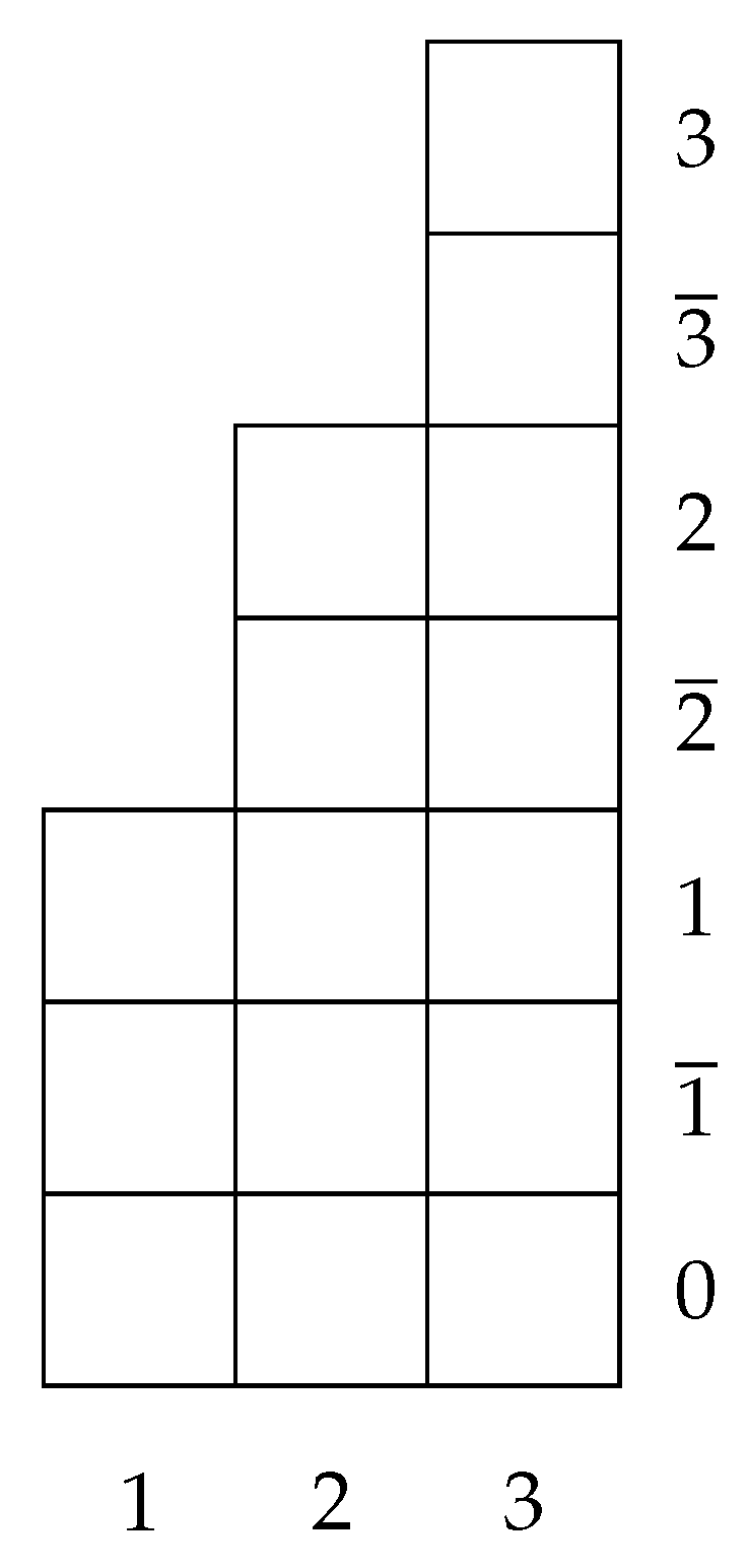
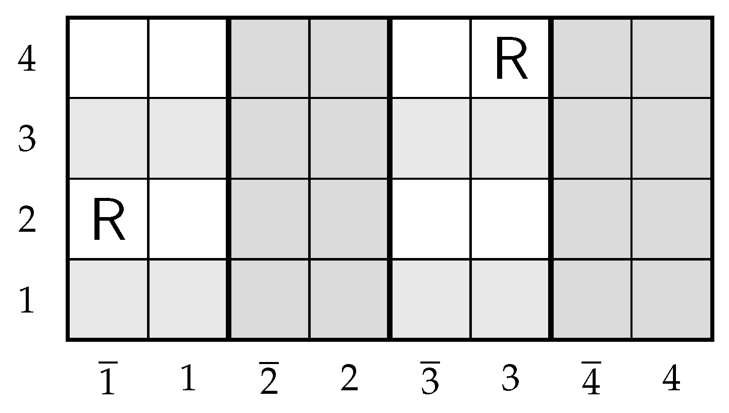
Remark 2.

Arranging the rows according to the level order ${<}_{\mathrm{lev}}$ gives a Ferrers-shaped board in which column i consists of the first $2i+1$ rows. The resulting staircase form is similar to that of a classical Ferrers diagram (see [10]). However, the signed row labels and the use of the level order make ${\mathcal{F}}_n^{\left(B\right)}$ different from the Ferrers boards studied in classical rook theory.

Thus, ${\mathcal{F}}_n^{\left(B\right)}$ can be viewed as a type B analogue of a Ferrers board adapted to signed restricted growth functions. The term level refers only to the ordering of signed rows and has no connection with the m-level rook placements considered in classical rook theory (see [9]).

Example 1.

Let $n=3$. The Ferrers board of type B${\mathcal{F}}_3^{\left(B\right)}$ has three columns. Column 1 contains the rows $\{0,\overline{1},1\}$, column 2 contains the rows $\{0,\overline{1},1,\overline{2},2\}$, and column 3 contains the rows $\{0,\overline{1},1,\overline{2},2,\overline{3},3\}$.

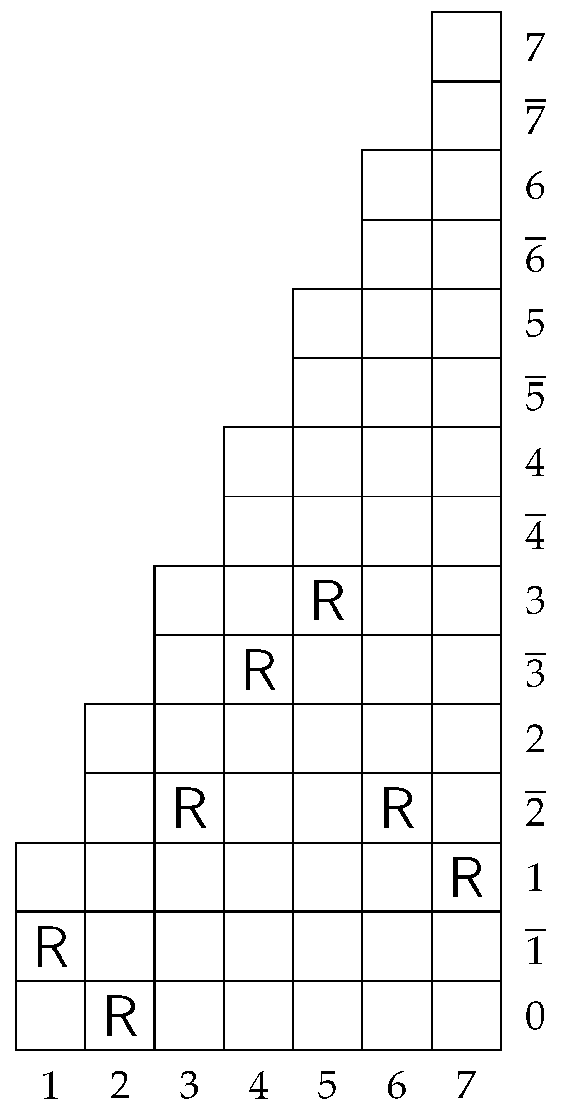
Ordering the rows according to the level order

$$0{<}_{\mathrm{lev}}\overline{1}{<}_{\mathrm{lev}}1{<}_{\mathrm{lev}}\overline{2}{<}_{\mathrm{lev}}2{<}_{\mathrm{lev}}\overline{3}{<}_{\mathrm{lev}}3,$$

the resulting board has a Ferrers shape with column heights $3,5,$ and 7, which is illustrated in Figure 1.

We now define type B rook placements on ${\mathcal{F}}_n^{\left(B\right)}$ and establish a natural bijection with signed restricted growth functions.

3.2. Rook Placements and Deletion Rules

Definition 2.

Let ${\mathcal{T}}_n^{\left(B\right)}$ denote the set of type B rook placements of size n on ${\mathcal{F}}_n^{\left(B\right)}$. Such a placement has the form

$$P=\{(r_i,i):1\le i\le n\},$$

where the following conditions hold. These conditions are the rook-theoretic counterparts of the signed restricted growth constraints and will be used to establish the correspondence with SRGF.

• Each column i contains exactly one rook, placed in a row $r_i\in \{0,\overline{1},1,\overline{2},2,\dots ,\overline{i},i\}$. No restriction is imposed on the rows, and distinct rooks may occupy the same row.
• The sequence $(r_1,\dots ,r_n)$ satisfies the type B signed restricted growth condition:

  $$|r_1|\in \{0,1\},|r_i|\le 1+max\{|r_1|,\dots ,|r_{i-1}\left|\right\}\mathit{for}i\ge 2.$$
• (Negative-before-positive rule.) For each $j\in \{1,\dots ,n\}$, if both $\overline{j}$ and j occur among $r_1,\dots ,r_n$, then the leftmost occurrence of $\overline{j}$ appears in a column strictly to the left of the leftmost occurrence of j.

We now establish the correspondence between signed restricted growth functions and rook placements of type B.

The next result shows that the combinatorial constraints defining type B rook placements coincide with those satisfied by signed restricted growth functions.

Proposition 1.

Let $w=a_0{a}_1{a}_1^{*}{a}_2{a}_2^{*}\cdots a_n{a}_n^{*}\in {\mathrm{SRGF}}_n$. Define

$$\Phi :{\mathrm{SRGF}}_n⟶{\mathcal{T}}_n^{\left(B\right)}\mathit{by}\Phi \left(w\right)=\{(a_i,i):1\le i\le n\},$$

Then, Φ is a bijection between ${\mathrm{SRGF}}_n$ and ${\mathcal{T}}_n^{\left(B\right)}$.

Proof. 

Let $w=a_0{a}_1{a}_1^{*}\dots a_n{a}_n^{*}\in {\mathrm{SRGF}}_n.$ By the signed restricted growth condition, $|a_i|\le i$ for each $1\le i\le n$, and hence $a_i\in \{0,\overline{1},1,\dots ,\overline{i},i\}$. Thus, the cell $(a_i,i)$ lies in column i of ${\mathcal{F}}_n^{\left(B\right)}$, and $\Phi \left(w\right)$ places exactly one rook in each column. The sequence $(a_1,\dots ,a_n)$ satisfies the signed restricted growth condition and the negative-before-positive rule, which are precisely the defining conditions of ${\mathcal{T}}_n^{\left(B\right)}$; hence, $\Phi \left(w\right)\in {\mathcal{T}}_n^{\left(B\right)}$.

For injectivity, by considering the definition of ${\mathrm{SRGF}}_n$, we note that starred entries are uniquely determined by the unstarred sequence $(a_1,\dots ,a_n)$, and thus w is uniquely determined by $(a_1,\dots ,a_n)$. If $\Phi \left(w\right)=\Phi \left(w^{\prime }\right)$, then $a_i=a_i^{\prime }$ for all i, so $w=w^{\prime }$. Therefore, Φ is injective.

For surjectivity, let $P={\left\{(r_i,i)\right\}}_{i=1}^n\in {\mathcal{T}}_n^{\left(B\right)}$. Define w by $a_0=0$, $a_i=r_i$ for $1\le i\le n$, and

$$a_i^{*}=\left\{\begin{array}{cc}0,\hfill & a_i=0,\hfill \\ \overline{a_i},\hfill & a_i\ne 0.\hfill \end{array}\right.$$

Since $P\in {\mathcal{T}}_n^{\left(B\right)}$, the sequence $(a_1,\dots ,a_n)=(r_1,\dots ,r_n)$ satisfies the signed restricted growth condition and the negative-before-positive rule. Hence, $w\in {\mathrm{SRGF}}_n$, and by construction $\Phi \left(w\right)=P$. Therefore, Φ is surjective and hence a bijection. □

Define ${\Phi }^{-1}:{\mathcal{T}}_n^{\left(B\right)}\to {\mathrm{SRGF}}_n$ by

$${\Phi }^{-1}\left({\left\{(r_i,i)\right\}}_{i=1}^n\right)=a_0{a}_1{a}_1^{*}{a}_2{a}_2^{*}\cdots a_n{a}_n^{*},$$

where $a_0=0$, $a_i=r_i$ for $1\le i\le n$, and

$$a_i^{*}=\left\{\begin{array}{cc}0,\hfill & a_i=0,\hfill \\ \overline{a_i},\hfill & a_i\ne 0.\hfill \end{array}\right.$$

Then, the resulting word belongs to ${\mathrm{SRGF}}_n$ and ${\Phi }^{-1}$ is thus well defined.

Remark 3.

The type B Ferrers board and the associated rook placements provide a geometric interpretation of signed restricted growth functions. Although the bijection is direct, viewing these functions on a board makes their structure easier to see. In particular, the board setting gives a clear framework for defining the statistics that lead to the $(p,q)$-Stirling polynomials of type B, together with their recurrence relations and generating functions.

Example 2.

Let $n=3$ and consider the signed restricted growth function

$$w=a_0{a}_1{a}_1^{*}{a}_2{a}_2^{*}{a}_3{a}_3^{*}=0\overline{1}100\overline{2}2\in {\mathrm{SRGF}}_3.$$

The unstarred sequence is

$$(a_1,a_2,a_3)=(\overline{1},0,\overline{2}).$$

Applying Φ, we obtain the rook placement

$$\Phi \left(w\right)=\{(\overline{1},1),(0,2),(\overline{2},3)\}\in {\mathcal{T}}_3^{\left(B\right)}.$$

Starting from this placement, one recovers w by setting $a_0=0$, $a_i=r_i$ for $1\le i\le 3$ and defining the starred entries accordingly.

We now present a larger example, which will serve as a running example throughout the remainder of the paper.

Example 3.

Consider the signed restricted growth function

$$w=a_0{a}_1{a}_1^{*}\cdots a_7{a}_7^{*}=0\overline{1}100\overline{2}2\overline{3}33\overline{3}\overline{2}21\overline{1}\in {\mathrm{SRGF}}_7.$$

The unstarred sequence is

$$(a_1,\dots ,a_7)=(\overline{1},0,\overline{2},\overline{3},3,\overline{2},1).$$

The corresponding rook placement on ${\mathcal{F}}_7^{\left(B\right)}$ is

$$\Phi \left(w\right)=\{(\overline{1},1),(0,2),(\overline{2},3),(\overline{3},4),(3,5),(\overline{2},6),(1,7)\}\in {\mathcal{T}}_7^{\left(B\right)}.$$

This rook placement is illustrated in Figure 2. Conversely, starting from

$$P=\{(r_i,i):1\le i\le 7\},$$

we recover the word by setting $a_0=0$ and $a_i=r_i$ for $1\le i\le 7$, with the starred entries determined by reversing the sign of $a_i$ (and $0^{*}=0$).

In particular,

$${\Phi }^{-1}\left(P\right)=0\overline{1}100\overline{2}2\overline{3}33\overline{3}\overline{2}21\overline{1}=w.$$

This illustrates both directions of the bijection in Proposition 1.

To obtain a $(p,q)$-refinement of the type B Stirling numbers, we introduce signed statistics on signed restricted growth functions. The restriction to first absolute occurrences reflects the block structure of signed partitions.

Definition 3.

Let $w=a_0{a}_1{a}_1^{*}{a}_2{a}_2^{*}\cdots a_n{a}_n^{*}\in {\mathrm{SRGF}}_n.$ The leftmost absolute set of w is defined by

$$L_B\left(w\right):=\left\{j\in \left[n\right]:|a_i|\ne |a_j|\mathrm{for}\mathrm{all}i<j\right\}.$$

Equivalently, $j\in L_B\left(w\right)$ if the absolute value $|a_j|$ appears for the first time at position j.

Example 4.

Consider the running example

$$w=0\overline{1}100\overline{2}2\overline{3}33\overline{3}\overline{2}21\overline{1}.$$

The main positions are

$$(a_1,\cdots ,a_7)=(\overline{1},0,\overline{2},\overline{3},3,\overline{2},1).$$

Their absolute values are

$$(1,0,2,3,3,2,1).$$

The first occurrence of 1 is at position 1, the first occurrence of 0 at position 2, the first occurrence of 2 at position 3, and the first occurrence of 3 at position 4. Hence,

$$L_B\left(w\right)=\{1,2,3,4\}.$$

Thus, the indices in $L_B\left(w\right)$ serve as reference positions in the level comparisons below. We now define the corresponding signed level statistics of type B.

Definition 4.

For $w\in {\mathrm{SRGF}}_n$ and each $i\in \left[n\right]$, we define

$$l{b}_i^B\left(w\right):=\#\left\{j\in L_B\left(w\right):j<i,a_j{>}_{\mathrm{lev}}{a}_i\right\},$$

$$l{s}_i^B\left(w\right):=\#\left\{j\in L_B\left(w\right):j<i,a_j{<}_{\mathrm{lev}}{a}_i\right\}.$$

The corresponding level-weighted statistics are

$${\mathrm{levLB}}_B\left(w\right):=\sum _{i=1}^{n}l{b}_i^B\left(w\right)|a_i|,\mathit{and}{\mathrm{levLS}}_B\left(w\right):=\sum _{i=1}^{n}l{s}_i^B\left(w\right)\left|a_i\right|.$$

These statistics depend only on the underlying sequence $(a_1,\dots ,a_n)$ of main entries and are independent of the starred components of w.

They extend the inversion statistics of Wachs and White [7] to the type B setting. For each i, the statistics $l{b}_i^B\left(w\right)$ and $l{s}_i^B\left(w\right)$ measure how the level of $a_i$ compares, in the signed level order, with the preceding levels. The weighted sums ${\mathrm{levLB}}_B\left(w\right)$ and ${\mathrm{levLS}}_B\left(w\right)$ multiply each contribution by $|a_i|$, yielding the refinement that appears in the $(p,q)$-Stirling polynomials of type B.

Example 5.

For the running example $w=0\overline{1}100\overline{2}2\overline{3}33\overline{3}\overline{2}21\overline{1},$ the main positions are

$$(a_1,\dots ,a_7)=(\overline{1},0,\overline{2},\overline{3},3,\overline{2},1).$$

Fix the level order

$$0{<}_{\mathrm{lev}}\overline{1}{<}_{\mathrm{lev}}1{<}_{\mathrm{lev}}\overline{2}{<}_{\mathrm{lev}}2{<}_{\mathrm{lev}}\overline{3}{<}_{\mathrm{lev}}3.$$

As computed in Example 4, we have

$$L_B\left(w\right)=\{1,2,3,4\}.$$

For each $i\in \left[7\right]$, we compute $l{b}_i^B\left(w\right)$ and $l{s}_i^B\left(w\right)$ by comparing $a_i$ only with the earlier entries $a_j$ for $j\in L_B\left(w\right)$. The values of $l{b}_i^B\left(w\right)$ and $l{s}_i^B\left(w\right)$ are summarised in

Table 1. Values of $l{b}_i^B\left(w\right)$ and $l{s}_i^B\left(w\right)$ for the running example $w=0\overline{1}100\overline{2}2\overline{3}33\overline{3}\overline{2}21\overline{1}$.

i	${\mathit{a}}_{\mathit{i}}$	$|{\mathit{a}}_{\mathit{i}}|$	${\mathit{lb}}_{\mathit{i}}^{\mathit{B}}\left(\mathit{w}\right)$	${\mathit{ls}}_{\mathit{i}}^{\mathit{B}}\left(\mathit{w}\right)$
1	$\overline{1}$	1	0	0
2	0	0	1	0
3	$\overline{2}$	2	0	2
4	$\overline{3}$	3	0	3
5	3	3	0	4
6	$\overline{2}$	2	1	2
7	1	1	2	2

. For illustration, we compute one representative case. For $i=6$, we have $a_6=\overline{2}$. We compare $a_6$ with the earlier entries $a_j$ for $j\in L_B\left(w\right)=\{1,2,3,4\}$ and $j<6$. With respect to the level order,

$$a_1=\overline{1}{<}_{\mathrm{lev}}\overline{2},a_2=0{<}_{\mathrm{lev}}\overline{2},a_3=\overline{2},a_4=\overline{3}{>}_{\mathrm{lev}}\overline{2}.$$

Thus, only $a_4$ contributes to $l{b}_6^B\left(w\right)$, while $a_1$ and $a_2$ contribute to $l{s}_6^B\left(w\right)$ (since they are strictly smaller in the level order). The equality $a_3=\overline{2}$ does not contribute to either count. Hence, $l{b}_6^B\left(w\right)=1$ and $l{s}_6^B\left(w\right)=2$. The remaining entries are computed similarly.

Consequently,

$$\begin{array}{cc}\hfill {\mathrm{levLB}}_B\left(w\right)& =\sum _{i=1}^{7}l{b}_i^B\left(w\right)\left|a_i\right|\hfill \\ & =l{b}_6^B\left(w\right)|a_6|+l{b}_7^B\left(w\right)\left|a_7\right|\hfill \\ & =1·2+2·1\hfill \\ & =4,\hfill \end{array}$$

and

$$\begin{array}{cc}\hfill {\mathrm{levLS}}_B\left(w\right)& =\sum _{i=1}^{7}l{s}_i^B\left(w\right)\left|a_i\right|\hfill \\ & =2·2+3·3+4·3+2·2+2·1\hfill \\ & =31.\hfill \end{array}$$

We now give a geometric interpretation of the signed statistics defined above in terms of rook placements on the type B Ferrers board ${\mathcal{F}}_n^{\left(B\right)}$. More precisely, we introduce type B rook statistics via a weak deletion procedure and show that they correspond to the SRGF statistics under the bijection Φ defined in Proposition 1.

Definition 5.

Let $P=\{(r_i,i):1\le i\le n\}\in {\mathcal{T}}_n^{\left(B\right)}$ be a type B rook placement on the Ferrers board ${\mathcal{F}}_n^{\left(B\right)}$.

• Leftmost absolute columns. We define the set of leftmost absolute columns by

  $$L_B\left(P\right):=\left\{j\in \left[n\right]:|r_i|\ne |r_j|\mathit{for}\mathit{all}i<j\right\}.$$

  Only rooks located in columns belonging to $L_B\left(P\right)$ perform deletions.
• South–East (SE-type) deletions. For each $j\in L_B\left(P\right)$, the rook $(r_j,j)$ deletes all cells $(t,k)\in {\mathcal{F}}_n^{\left(B\right)}$ satisfying

  $$k>j\mathit{and}t{<}_{\mathrm{lev}}{r}_j.$$

  That is, deletions occur only in columns to the right of column j and below the level of $r_j$.
• SE-hit numbers. For each $i\in \left[n\right]$, we define

  $${\delta }_i^{SE}\left(P\right):=\#\left\{j\in L_B\left(P\right):j<i\mathit{such}\mathit{that}\mathit{the}\mathit{rook}(r_i,i)\mathit{is}\mathit{deleted}\mathit{by}\mathit{the}\mathit{SE-deletion}\mathit{from}\mathit{column}j\right\}.$$
• Level-weighted SE statistic. We then define the level-weighted SE statistic by

  $${\mathrm{levSE}}_B\left(P\right):=\sum _{i=1}^n{\delta }_i^{SE}\left(P\right)\left|r_i\right|.$$
• North–East (NE-type) deletions. Similarly, for each $j\in L_B\left(P\right)$, the rook $(r_j,j)$ deletes all cells $(t,k)\in {\mathcal{F}}_n^{\left(B\right)}$ satisfying

  $$k>j\mathit{and}{r}_j{<}_{\mathrm{lev}}t.$$

  Defining ${\delta }_i^{NE}\left(P\right)$ in the same way, we obtain

  $${\mathrm{levNE}}_B\left(P\right):=\sum _{i=1}^n{\delta }_i^{NE}\left(P\right)\left|r_i\right|.$$

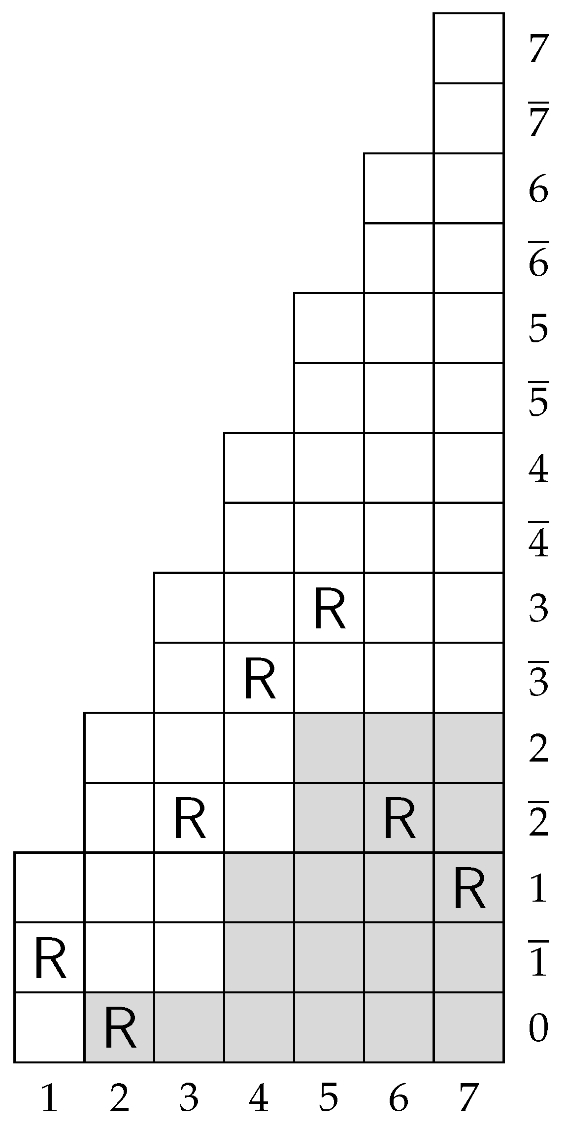
Remark 4.

Although our deletion procedure is inspired by the work of Wachs and White (see [7]), the statistics considered here are different in a fundamental way. Instead of counting undeleted cells, we record how many earlier deletion regions remove the rook cell in each column. This approach is natural in the type B setting, where signed comparisons and first occurrences of absolute values are fundamental.

Example 6.

Continuing with the running example

$$w=0\overline{1}100\overline{2}2\overline{3}33\overline{3}\overline{2}21\overline{1},$$

let

$$P=\Phi \left(w\right)\in {\mathcal{T}}_7^{\left(B\right)}$$

be the associated type B rook placement on the Ferrers board ${\mathcal{F}}_7^{\left(B\right)}$. The rook rows are

$$(r_1,\dots ,r_7)=(\overline{1},0,\overline{2},\overline{3},3,\overline{2},1).$$

• Step 1: Leftmost absolute columns. The absolute values of the rook rows are

  $$\left(\right|r_1|,\dots ,|r_7\left|\right)=(1,0,2,3,3,2,1).$$

  The first occurrences of the absolute values $1,0,2,$ and 3 appear in columns $1,2,3,$ and 4, respectively. Hence,

  $$L_B\left(P\right)=\{1,2,3,4\}.$$

  Only the rooks in these columns perform deletions.
• Step 2: SE-deletions. We apply the SE-type deletion procedure column by column.
  • The rook $(\overline{1},1)$ deletes all cells $(t,k)$ with $k>1$ and $t{<}_{\mathrm{lev}}\overline{1}$, i.e., all cells in row 0 in columns 2 through 7.
  • The rook $(0,2)$ deletes no cells, since there are no rows strictly below 0 in the type B order.
  • The rook $(\overline{2},3)$ deletes all cells in rows $\{0,\overline{1},1\}$ in columns 4 through 7.
  • The rook $(\overline{3},4)$ deletes all cells in rows $\{0,\overline{1},1,\overline{2},2\}$ in columns 5 through 7.

The resulting SE-deletions are illustrated in Figure 3.

• Step 3: SE/NE-hit numbers. For each column i, we compute the numbers ${\delta }_i^{SE}\left(P\right)$ and ${\delta }_i^{NE}\left(P\right)$, which count how many earlier distinguished columns delete the rook cell $(r_i,i)$ under the SE and NE rules, respectively. The results are summarised in

  Table 2. Deletion statistics ${\delta }_i^{SE}\left(P\right)$ and ${\delta }_i^{NE}\left(P\right)$ for the rook placement $P=\Phi \left(w\right)$ corresponding to the running example w on ${\mathcal{F}}_7^{\left(B\right)}$.

  i	${\mathit{r}}_{\mathit{i}}$	${\mathit{\delta }}_{\mathit{i}}^{\mathit{SE}}\left(\mathit{P}\right)$	${\mathit{\delta }}_{\mathit{i}}^{\mathit{NE}}\left(\mathit{P}\right)$
  1	$\overline{1}$	0	0
  2	0	1	0
  3	$\overline{2}$	0	2
  4	$\overline{3}$	0	3
  5	3	0	4
  6	$\overline{2}$	1	2
  7	1	2	2

  .

Thus,

$$({\delta }_1^{SE},\dots ,{\delta }_7^{SE})=(0,1,0,0,0,1,2),({\delta }_1^{NE},\dots ,{\delta }_7^{NE})=(0,0,2,3,4,2,2).$$

• Step 4: Level-weighted SE statistic. We compute

  $${\mathrm{levSE}}_B\left(P\right)=\sum _{i=1}^7{\delta }_i^{SE}\left(P\right)\left|r_i\right|.$$

  Only the indices $i=2,6,7$ contribute nonzero terms to the sum. Since

  $$|r_2|=0,|r_6|=2,|r_7|=1,$$

  we obtain

  $${\mathrm{levSE}}_B\left(P\right)=(1·0)+(1·2)+(2·1)=4.$$

  The NE-hit numbers are obtained analogously, using the condition $r_j{<}_{\mathrm{lev}}{r}_i$ and are recorded in the last column of Table 2.
• Step 5: Level-weighted NE statistic. We compute

  $${\mathrm{levNE}}_B\left(P\right)=\sum _{i=1}^7{\delta }_i^{NE}\left(P\right)\left|r_i\right|.$$

  Since $|r_3|=2$, $|r_4|=3$, $|r_5|=3$, $|r_6|=2$, and $|r_7|=1$, we obtain

  $${\mathrm{levNE}}_B\left(P\right)=(2·2)+(3·3)+(4·3)+(2·2)+(2·1)=31.$$

Lemma 1.

Let $w\in {\mathrm{SRGF}}_n$ and set $P=\Phi \left(w\right)\in {\mathcal{T}}_n^{\left(B\right)}$. Then,

$${\mathrm{levLB}}_B\left(w\right)={\mathrm{levSE}}_B\left(P\right)\mathit{and}{\mathrm{levLS}}_B\left(w\right)={\mathrm{levNE}}_B\left(P\right).$$

Proof. 

Let $w=a_0{a}_1{a}_1^{*}\cdots a_n{a}_n^{*}\in {\mathrm{SRGF}}_n\mathrm{and}P=\Phi \left(w\right)=\{(r_i,i):1\le i\le n\}.$ From the definition of the bijection Φ, we have $r_i=a_i$ for all $1\le i\le n$. In particular, the sets of leftmost absolute positions coincide:

$$L_B\left(P\right)=\{j\in \left[n\right]:|r_i|\ne |r_j|\mathrm{for}\mathrm{all}i<j\}=\{j\in \left[n\right]:|a_i|\ne |a_j|\mathrm{for}\mathrm{all}i<j\}=L_B\left(w\right).$$

Fix $i\in \left[n\right]$. For each $j\in L_B\left(P\right)$, the SE-deletion removes precisely those cells $(t,k)$ with $k>j$ and $t{<}_{\mathrm{lev}}{r}_j$. In particular, the rook cell $(r_i,i)$ is deleted by the SE-deletion from column j if and only if $j<i$ and $r_i{<}_{\mathrm{lev}}{r}_j$, or equivalently, $r_j{>}_{\mathrm{lev}}{r}_i$. It follows that

$${\delta }_i^{SE}\left(P\right)=\#\{j\in L_B\left(P\right):j<i,r_j{>}_{\mathrm{lev}}{r}_i\}=\#\{j\in L_B\left(w\right):j<i,a_j{>}_{\mathrm{lev}}{a}_i\}=l{b}_i^B\left(w\right).$$

Multiplying both sides by $|r_i|=|a_i|$ and summing over all i yields

$${\mathrm{levSE}}_B\left(P\right)=\sum _{i=1}^n{\delta }_i^{SE}\left(P\right)|r_i|=\sum _{i=1}^{n}l{b}_i^B\left(w\right)\left|a_i\right|={\mathrm{levLB}}_B\left(w\right).$$

Similarly, the NE-deletion from column j removes those cells $(t,k)$ with $k>j$ and $r_j{<}_{\mathrm{lev}}t$. Hence, the rook cell $(r_i,i)$ is deleted by this deletion if and only if $j<i$ and $r_j{<}_{\mathrm{lev}}{r}_i$. It follows that

$${\delta }_i^{NE}\left(P\right)=\#\{j\in L_B\left(P\right):j<i,r_j{<}_{\mathrm{lev}}{r}_i\}=l{s}_i^B\left(w\right),$$

and therefore

$${\mathrm{levNE}}_B\left(P\right)={\mathrm{levLS}}_B\left(w\right).$$

This completes the proof. □

3.3. $(p,q)$-Stirling Polynomials of Type B

We now introduce the $(p,q)$-Stirling polynomials of type B. We define ${\mathrm{SRGF}}_{n,k}$ to be the set of signed restricted growth functions $w\in {\mathrm{SRGF}}_n$ such that

$$\underset{1\le i\le n}{max}\left|a_i\right|=k.$$

We define

$${\mathrm{SRGF}}_{n,k}^{(B,0)}=\{w\in {\mathrm{SRGF}}_{n,k}:0\notin \{a_1,\dots ,a_n\}\},$$

and

$${\mathrm{SRGF}}_{n,k}^{(B,1)}=\{w\in {\mathrm{SRGF}}_{n,k}:0\in \{a_1,\dots ,a_n\}\},$$

where $w=a_0{a}_1{a}_1^{*}{a}_2{a}_2^{*}\cdots a_n{a}_n^{*}$.

On the rook side, we define ${\mathcal{T}}_{n,k}^{\left(B\right)}$ to be the set of rook placements $P\in {\mathcal{T}}_n^{\left(B\right)}$ such that

$$\underset{1\le i\le n}{max}\left|a_i\right|=k.$$

Definition 6.

For $n\ge 1$ and $0\le k\le n$, we define the $(p,q)$-Stirling polynomials of type B by

$$S_{p,q}^{\left(B\right)}(n,k)=\sum _{w\in {\mathrm{SRGF}}_{n,k}}{q}^{{\mathrm{levLB}}_B\left(w\right)}{p}^{{\mathrm{levLS}}_B\left(w\right)}.$$

Remark 5.

The polynomials $S_{p,q}^{\left(B\right)}(n,k)$ may be viewed as a $(p,q)$-refinement of the type B Stirling numbers. When $p=q=1$, we obtain the classical counting of signed set partitions with k blocks. The parameters p and q record the joint distribution of two signed, level-weighted statistics measuring left and right interactions.

For illustration, we compute $S_{p,q}^{\left(B\right)}(3,2)$ explicitly.

Table 3. Distribution of the statistics ${\mathrm{levLB}}_B\left(w\right)$ and ${\mathrm{levLS}}_B\left(w\right)$ over ${\mathrm{SRGF}}_{3,2}$.

w	$({\mathit{lb}}_1^{\mathit{B}},{\mathit{lb}}_2^{\mathit{B}},{\mathit{lb}}_3^{\mathit{B}})$	$({\mathit{ls}}_1^{\mathit{B}},{\mathit{ls}}_2^{\mathit{B}},{\mathit{ls}}_3^{\mathit{B}})$	${\mathbf{levLB}}_{\mathit{B}}\left(\mathit{w}\right)$	${\mathbf{levLS}}_{\mathit{B}}\left(\mathit{w}\right)$
$000\overline{1}1\overline{2}2$	$(0,0,0)$	$(0,1,2)$	0	5
$000\overline{1}12\overline{2}$	$(0,0,0)$	$(0,1,2)$	0	5
$0001\overline{1}\overline{2}2$	$(0,0,0)$	$(0,1,2)$	0	5
$0001\overline{1}2\overline{2}$	$(0,0,0)$	$(0,1,2)$	0	5
$0\overline{1}100\overline{2}2$	$(0,1,0)$	$(0,0,2)$	0	4
$0\overline{1}1002\overline{2}$	$(0,1,0)$	$(0,0,2)$	0	4
$0\overline{1}1\overline{1}1\overline{2}2$	$(0,0,0)$	$(0,0,1)$	0	2
$0\overline{1}1\overline{1}12\overline{2}$	$(0,0,0)$	$(0,0,1)$	0	2
$0\overline{1}11\overline{1}\overline{2}2$	$(0,0,0)$	$(0,1,1)$	0	3
$0\overline{1}11\overline{1}2\overline{2}$	$(0,0,0)$	$(0,1,1)$	0	3
$0\overline{1}1\overline{2}200$	$(0,0,2)$	$(0,1,0)$	0	2
$0\overline{1}1\overline{2}2\overline{1}1$	$(0,0,1)$	$(0,1,0)$	1	2
$0\overline{1}1\overline{2}21\overline{1}$	$(0,0,1)$	$(0,1,1)$	1	3
$0\overline{1}1\overline{2}2\overline{2}2$	$(0,0,0)$	$(0,1,1)$	0	4
$0\overline{1}1\overline{2}22\overline{2}$	$(0,0,0)$	$(0,1,2)$	0	6
$0\overline{1}12\overline{2}00$	$(0,0,2)$	$(0,1,0)$	0	2
$0\overline{1}12\overline{2}\overline{1}1$	$(0,0,1)$	$(0,1,0)$	1	2
$0\overline{1}12\overline{2}1\overline{1}$	$(0,0,1)$	$(0,1,1)$	1	3
$0\overline{1}12\overline{2}2\overline{2}$	$(0,0,0)$	$(0,1,1)$	0	4
$01\overline{1}00\overline{2}2$	$(0,1,0)$	$(0,0,2)$	0	4
$01\overline{1}002\overline{2}$	$(0,1,0)$	$(0,0,2)$	0	4
$01\overline{1}1\overline{1}\overline{2}2$	$(0,0,0)$	$(0,0,1)$	0	2
$01\overline{1}1\overline{1}2\overline{2}$	$(0,0,0)$	$(0,0,1)$	0	2
$01\overline{1}\overline{2}200$	$(0,0,2)$	$(0,1,0)$	0	2
$01\overline{1}\overline{2}21\overline{1}$	$(0,0,1)$	$(0,1,0)$	1	2
$01\overline{1}\overline{2}2\overline{2}2$	$(0,0,0)$	$(0,1,1)$	0	4
$01\overline{1}\overline{2}22\overline{2}$	$(0,0,0)$	$(0,1,2)$	0	6
$01\overline{1}2\overline{2}00$	$(0,0,2)$	$(0,1,0)$	0	2
$01\overline{1}2\overline{2}1\overline{1}$	$(0,0,1)$	$(0,1,0)$	1	2
$01\overline{1}2\overline{2}2\overline{2}$	$(0,0,0)$	$(0,1,1)$	0	4

lists the elements of ${\mathrm{SRGF}}_{3,2}$ together with their statistics and corresponding weights.

From Table 3, we obtain

$$S_{p,q}^{\left(B\right)}(3,2)=8p^2+2p^3+8p^4+4p^5+2p^6+q(4p^2+2p^3).$$

For small values of n and k, the $(p,q)$-Stirling polynomials of type B can be computed explicitly. We record these values in

Table 4. Explicit values of the $(p,q)$-Stirling polynomials of type B, $S_{p,q}^{\left(B\right)}(n,k)$, for $1\le n,k\le 5$.

$\mathit{n}\setminus \mathit{k}$	1	2	3	4	5
1	2
2	$4+3p$	$4p^2$
3	$6+9p+4p^2+p^3$	$8p^2+2p^3+8p^4+4p^5$ $+2p^6+q\left(4p^2+2p^3\right)$	$8p^8$
4	$\begin{array}{cc}& 8+18p+16p^2\hfill \\ & +9p^3+3p^4+p^5\hfill \end{array}$	$\begin{array}{cc}& 12p^2+6p^3+22p^4+20p^5\hfill \\ & +18p^6+3p^7+10p^8+4p^9\hfill \\ & +4p^{10}+2p^{11}+q(8p^2+10p^3\hfill \\ & +12p^4+8p^5+10p^6+4p^7)\hfill \\ & +q^2\left(4p^2+4p^3+2p^4\right)\hfill \end{array}$	$\begin{array}{cc}& 16p^8+4p^9+8p^{10}+8p^{11}\hfill \\ & +4p^{12}+8p^{13}+16p^{14}+4p^{17}\hfill \\ & +q\left(8p^8+4p^9\right)\hfill \\ & +q^2\left(8p^8+4p^9+8p^{10}+4p^{12}\right)\hfill \end{array}$	$16p^{20}$
5	$\begin{array}{cc}& 10+30p+40p^2+35p^3\hfill \\ & +21p^4+11p^5+4p^6+p^7\hfill \end{array}$	$\begin{array}{cc}& 16p^2+12p^3+44p^4+56p^5\hfill \\ & +60p^6+25p^7+45p^8+27p^9\hfill \\ & +32p^{10}+14p^{11}+19p^{12}+5p^{13}\hfill \\ & +8p^{14}+4p^{15}+2p^{16}+2p^{17}\hfill \\ & +q(12p^2+24p^3+32p^4+36p^5\hfill \\ & +60p^6+42p^7+27p^8+21p^9\hfill \\ & +20p^{10}+11p^{11}+6p^{12}+2p^{13})\hfill \\ & +q^2(8p^2+14p^3+28p^4+20p^5\hfill \\ & +18p^6+14p^7+9p^8+2p^9)\hfill \\ & +q^3\left(4p^2+6p^3+6p^4+2p^5\right)\hfill \end{array}$	$\begin{array}{cc}& 24p^8+12p^9+20p^{10}+28p^{11}\hfill \\ & +20p^{12}+42p^{13}+68p^{14}+28p^{15}\hfill \\ & +16p^{16}+28p^{17}+14p^{18}+8p^{19}\hfill \\ & +24p^{20}+2p^{21}+8p^{22}+20p^{23}\hfill \\ & +4p^{25}+8p^{26}+q(16p^8+12p^9\hfill \\ & +20p^{10}+16p^{11}+20p^{12}+8p^{13}\hfill \\ & +16p^{14}+16p^{15}+4p^{16}+4p^{17}\hfill \\ & +2p^{18})+q^2(24p^8+28p^9+36p^{10}\hfill \\ & +8p^{11}+36p^{12}+8p^{13}+36p^{14}\hfill \\ & +28p^{15}+24p^{16}+20p^{17}+20p^{18}\hfill \\ & +12p^{19}+4p^{20}+4p^{21})+q^3(8p^8\hfill \\ & +8p^9+12p^{10}+4p^{11}+4p^{12}+2p^{13})\hfill \\ & +q^4(8p^8+8p^9+20p^{10}+8p^{11}\hfill \\ & +16p^{12}+4p^{13}+8p^{14}+4p^{16})\hfill \end{array}$	$\begin{array}{cc}& 32p^{20}+8p^{21}+16p^{22}+24p^{24}\hfill \\ & +16p^{26}+16p^{27}+24p^{29}+16p^{30}\hfill \\ & +16p^{32}+8p^{36}+q\left(8p^{21}+16p^{20}\right)\hfill \\ & +q^2\left(16p^{20}+8p^{21}+16p^{22}+8p^{24}\right)\hfill \\ & +q^3\left(16p^{20}+8p^{21}+16p^{26}+8p^{29}\right)\hfill \\ & +q^4\left(16p^{22}+8p^{24}\right)\hfill \end{array}$	$32p^{40}$

for $1\le n,k\le 5$.

Theorem 1.

For all n and k,

$$S_{p,q}^{\left(B\right)}(n,k)=\sum _{w\in {\mathrm{SRGF}}_{n,k}}{q}^{{\mathrm{levLB}}_B\left(w\right)}{p}^{{\mathrm{levLS}}_B\left(w\right)}=\sum _{P\in {\mathcal{T}}_{n,k}^{\left(B\right)}}{q}^{{\mathrm{levSE}}_B\left(P\right)}{p}^{{\mathrm{levNE}}_B\left(P\right)}.$$

Proof. 

By Proposition 1, the map Φ is a bijection from ${\mathrm{SRGF}}_{n,k}$ onto ${\mathcal{T}}_{n,k}^{\left(B\right)}$. Moreover, by Lemma 1, for every $w\in {\mathrm{SRGF}}_{n,k}$ we have

$${\mathrm{levLB}}_B\left(w\right)={\mathrm{levSE}}_B(\Phi \left(w\right))\mathrm{and}{\mathrm{levLS}}_B\left(w\right)={\mathrm{levNE}}_B(\Phi \left(w\right)).$$

Thus, Φ preserves the weight $q^{{\mathrm{levLB}}_B\left(w\right)}{p}^{{\mathrm{levLS}}_B\left(w\right)}$. Summing over all $w\in {\mathrm{SRGF}}_{n,k}$ therefore yields

$$\sum _{w\in {\mathrm{SRGF}}_{n,k}}{q}^{{\mathrm{levLB}}_B\left(w\right)}{p}^{{\mathrm{levLS}}_B\left(w\right)}=\sum _{P\in {\mathcal{T}}_{n,k}^{\left(B\right)}}{q}^{{\mathrm{levSE}}_B\left(P\right)}{p}^{{\mathrm{levNE}}_B\left(P\right)},$$

as claimed. □

To formulate recurrence relations for the polynomials $S_{p,q}^{\left(B\right)}(n,k)$, it is convenient to refine them according to the presence of 0 and the pattern of first sign occurrences.

Definition 7.

For $\epsilon \in \{0,1\}$, we define

$$S_{p,q}^{(B,\epsilon )}(n,k):=\sum _{\begin{array}{c}w\in {\mathrm{SRGF}}_{n,k}\\ 0\in \{a_1,\dots ,a_n\}\mathit{if}\mathit{and}\mathit{only}\mathit{if}\epsilon =1\end{array}}{q}^{{\mathrm{levLB}}_B\left(w\right)}{p}^{{\mathrm{levLS}}_B\left(w\right)}.$$

Thus, $S_{p,q}^{(B,0)}(n,k)$ counts words in ${\mathrm{SRGF}}_{n,k}$ whose main letters avoid 0, while $S_{p,q}^{(B,1)}(n,k)$ counts those in which 0 occurs among the main letters. In particular, we have

$$S_{p,q}^{\left(B\right)}(n,k)=S_{p,q}^{(B,0)}(n,k)+S_{p,q}^{(B,1)}(n,k).$$

We set $S_{p,q}^{(B,\epsilon )}(n,k)=0$ if $k<0$ or $k>n$. Moreover,

$$S_{p,q}^{(B,0)}(0,0)=1,S_{p,q}^{(B,1)}(0,0)=0,$$

and $S_{p,q}^{(B,\epsilon )}(0,k)=0$ for $k\ne 0$.

Definition 8.

For $w=a_1{a}_2\cdots a_n\in {\mathrm{SRGF}}_{n,k}$, we define

$$P\left(w\right):=\left\{j\in \left[k\right]:\mathit{the}\mathit{first}\mathit{occurrence}\mathit{of}\{j,\overline{j}\}\mathit{in}w\mathit{starts}\mathit{with}+j\right\}.$$

That is, $P\left(w\right)$ consists of those indices $j\in \left[k\right]$ whose first appearance in w occurs with positive sign. By the negative-before-positive rule, the condition $j\in P\left(w\right)$ implies that $\overline{j}$ does not occur as a main letter in w.

Definition 9.

For $\epsilon \in \{0,1\}$ and a subset $P\subseteq \left[k\right]$, we define

$$S_{p,q}^{(B,\epsilon )}(n,k;P):=\sum _{\begin{array}{c}w\in {\mathrm{SRGF}}_{n,k}^{(B,\epsilon )}\\ P\left(w\right)=P\end{array}}{q}^{{\mathrm{levLB}}_B\left(w\right)}{p}^{{\mathrm{levLS}}_B\left(w\right)}.$$

In other words, $S_{p,q}^{(B,\epsilon )}(n,k;P)$ records the contribution of those words in ${\mathrm{SRGF}}_{n,k}^{(B,\epsilon )}$ whose positive-first set is exactly P. Moreover,

$$S_{p,q}^{(B,\epsilon )}(n,k)=\sum _{P\subseteq \left[k\right]}{S}_{p,q}^{(B,\epsilon )}(n,k;P).$$

We illustrate this definition in the case $n=3$ and $k=2$. Using Table 3, we separate the words in ${\mathrm{SRGF}}_{3,2}$ according to whether 0 appears among the main letters. The words whose main letters avoid 0 contribute to $S_{p,q}^{(B,0)}(3,2)$. From the table, summing their corresponding weights gives

$$S_{p,q}^{(B,0)}(3,2)=4p^2+2p^3+4p^4+2p^6+q(4p^2+2p^3).$$

Similarly, the words in which 0 appears among the main letters contribute to $S_{p,q}^{(B,1)}(3,2)$. From Table 3, we obtain

$$S_{p,q}^{(B,1)}(3,2)=4p^2+4p^4+4p^5.$$

Consequently, we obtain

$$S_{p,q}^{\left(B\right)}(3,2)=S_{p,q}^{(B,0)}(3,2)+S_{p,q}^{(B,1)}(3,2)=8p^2+2p^3+8p^4+4p^5+2p^6+q(4p^2+2p^3).$$

Definition 10.

For $P\subseteq \left[k\right]$, we define

$$A_k(p,q;P):=\sum _{j=1}^k{q}^{(k-j)j}\left(p^{j(j-1)}+{\mathbf{1}}_{(j\notin P)}{p}^{j^2}\right),$$

(7)

$$B_k(p,q;P):=1+\sum _{j=1}^k{q}^{(k-j)j}\left(p^{j^2}+{\mathbf{1}}_{(j\notin P)}{p}^{j(j+1)}\right).$$

(8)

We are now in a position to give the recurrence relations for the refined $(p,q)$-Stirling polynomials of type B.

Theorem 2.

For $n\ge 1$, $1\le k\le n$, and $P\subseteq \left[k\right]$, the $(p,q)$-Stirling polynomials of type B satisfy the following recurrence relations.

• Zero absent. For $\epsilon =0$, we have

  $$S_{p,q}^{(B,0)}(n,k;P)=p^{k(k-1)}{S}_{p,q}^{(B,0)}\left(n-1,k-1;P\cap [k-1]\right)+A_k(p,q;P)S_{p,q}^{(B,0)}(n-1,k;P).$$

  (9)
• Zero present. For $\epsilon =1$, we have

  $$\begin{array}{cc}\hfill S_{p,q}^{(B,1)}(n,k;P)=p^{k^2}{S}_{p,q}^{(B,1)}\left(n-1,k-1;P\cap [k-1]\right)& +B_k(p,q;P)S_{p,q}^{(B,1)}(n-1,k;P)\hfill \\ \hfill & +S_{p,q}^{(B,0)}(n-1,k;P).\hfill \end{array}$$

  (10)

  where $A_k(p,q;P)$ and $B_k(p,q;P)$ are defined in Equations (7) and (8), respectively.

Proof. 

By the signed restricted growth condition in Equation (6), a word $w\in {\mathrm{SRGF}}_{n,k}$ cannot reach the maximum absolute value k without first realising every smaller absolute value. Hence, each of $1,2,\dots ,k$ appears at least once among the main letters of w. It follows that $L_B\left(w\right)$ contains exactly one representative for each absolute value $1,\dots ,k$ and possibly also the first occurrence of 0. We prove both recurrences by tracking whether the main letter 0 occurs. Let

$$w=a_0{a}_1{a}_1^{*}\cdots a_{n-1}{a}_{n-1}^{*}{a}_n{a}_n^{*}\in {\mathrm{SRGF}}_{n,k}$$

and let $w^{\prime }$ denote the initial segment of w obtained by deleting the final pair $(a_n,a_n^{*})$. We distinguish cases according to whether the absolute value $|a_n|$ is new, that is, does not appear among the integers $|a_1|,|a_2|,\dots ,|a_{n-1}|$.

• Case 1: $|a_n|=k$ is new. Then, $w^{\prime }\in {\mathrm{SRGF}}_{n-1,k-1}$ and $n\in L_B\left(w\right)$. Since all reference values have an absolute value of $k-1$ at most, they occur before both $\overline{k}$ and k in the type B level order. Hence,

  $$l{b}_n^B\left(w\right)=0,l{s}_n^B\left(w\right)=\left|L_B\left(w^{\prime }\right)\right|.$$

  Thus, the level-weighted statistics satisfy

  $${\mathrm{levLB}}_B\left(w\right)={\mathrm{levLB}}_B\left(w^{\prime }\right),{\mathrm{levLS}}_B\left(w\right)={\mathrm{levLS}}_B\left(w^{\prime }\right)+k\left|L_B\left(w^{\prime }\right)\right|.$$

If 0 is absent from $w^{\prime }$, then the reference set consists of the first occurrences of the absolute values $1,2,\dots ,k-1$, and therefore $|L_B\left(w^{\prime }\right)|=k-1$, yielding the factor $p^{k(k-1)}$. If 0 is present, then $|L_B\left(w^{\prime }\right)|=k$, yielding $p^{k^2}$. Since $|a_n|=k$ is new, the letter $a_n$ is the first occurrence of absolute value k. Thus, the condition $P\left(w\right)=P$ forces its sign: if $k\in P$, then $a_n=+k$, whereas if $k\notin P$, then $a_n=\overline{k}$. Finally, since the level k does not appear in $w^{\prime }$, we therefore have $P\left(w^{\prime }\right)=P\cap [k-1]$. This produces the first terms in the stated recurrences.

• Case 2: The maximum k already occurs in $w^{\prime }$. Then, $w^{\prime }\in {\mathrm{SRGF}}_{n-1,k}$. The reference set remains unchanged, with $L_B\left(w\right)=L_B\left(w^{\prime }\right)$, and the positive-first set is preserved: $P\left(w\right)=P\left(w^{\prime }\right)=P$.

Since $w^{\prime }\in {\mathrm{SRGF}}_{n-1,k}$, each absolute value $1,\dots ,k$ occurs in $w^{\prime }$, and hence $L_B\left(w^{\prime }\right)$ contains exactly one first occurrence for each of these values.

Fix $j\in \left[k\right]$ and choose $a_n$ with $|a_n|=j$. There are exactly $k-j$ reference absolute values larger than j, and therefore

$$l{b}_n^B\left(w\right)=k-j.$$

Consequently, each such choice contributes a factor $q^{(k-j)j}$, independently of the sign of $a_n$.

We now determine $l{s}_n^B\left(w\right)$. If $j\in P$, then by the negative-before-positive rule, the letter $\overline{j}$ never occurs in $w^{\prime }$, and the only admissible choice is $a_n=+j$. If $j\notin P$, then the first occurrence of $\left|j\right|$ is $\overline{j}$, and both signs $a_n=\overline{j}$ and $a_n=j$ are allowed.

Suppose that 0 is absent from $w^{\prime }$. In this case, the reference set contains exactly one representative for each absolute value $1,\dots ,k$. Choosing $a_n=\overline{j}$ yields $l{s}_n^B\left(w\right)=j-1$. If $a_n=+j$, then the number of smaller reference values depends on whether j belongs to the positive-first set, and we have

$$l{s}_n^B\left(w\right)=\left\{\begin{array}{cc}j-1,\hfill & \mathrm{if}j\in P,\hfill \\ j,\hfill & \mathrm{if}j\notin P.\hfill \end{array}\right.$$

Consequently, for fixed j, the total contribution is

$$q^{(k-j)j}\left(p^{j(j-1)}+{\mathbf{1}}_{(j\notin P)}{p}^{j^2}\right),$$

and summing over $j=1,\dots ,k$ yields the factor $A_k(p,q;P)$.

If 0 is present in $w^{\prime }$. In this case, 0 is an additional smaller reference value, so each of the preceding values of $l{s}_n^B\left(w\right)$ increases by 1. Thus, choosing $a_n$ to be either j or $\overline{j}$ contributes

$$q^{(k-j)j}\left(p^{j^2}+{\mathbf{1}}_{(j\notin P)}{p}^{j(j+1)}\right),$$

and the additional choice $a_n=0$ contributes weight 1. Summing over j yields the factor $B_k(p,q;P)$.

Finally, if $w^{\prime }\in {\mathrm{SRGF}}_{n-1,k}^{(B,0)}$, then choosing $a_n=0$ produces an element of ${\mathrm{SRGF}}_{n,k}^{(B,1)}$ without affecting the statistics, yielding the transition term $S_{p,q}^{(B,0)}(n-1,k;P)$.

Combining all cases completes the proof. □

We illustrate the recurrence relations in Theorem 2 with the following two examples, corresponding to the cases $\epsilon =1$ and $\epsilon =0$.

Example 7.

Let $n=3$ and $k=2$. We verify Equation (10) for ${\mathrm{SRGF}}_{3,2}^{(B,1)}$ with $P\left(w\right)=\left\{2\right\}$.

• Left-hand side. By Table 3, the words in ${\mathrm{SRGF}}_{3,2}^{(B,1)}$ with $P\left(w\right)=\left\{2\right\}$ are

  $$(0,\overline{1},2),(\overline{1},0,2),(\overline{1},2,0),$$

  with ${\mathrm{levLS}}_B\left(w\right)=5,4,2$, respectively. Hence,

  $$S_{p,q}^{(B,1)}(3,2;\left\{2\right\})=p^5+p^4+p^2.$$
• Right-hand side. Applying (10), we obtain

  $$S_{p,q}^{(B,1)}(3,2;\left\{2\right\})=p^4{S}_{p,q}^{(B,1)}(2,1;⌀)+S_{p,q}^{(B,0)}(2,2;\left\{2\right\}),$$

  since $S_{p,q}^{(B,1)}(2,2;\left\{2\right\})=0$. Hence, we obtain

  $$S_{p,q}^{(B,1)}(2,1;⌀)=p+1,S_{p,q}^{(B,0)}(2,2;\left\{2\right\})=p^2.$$

  Thus, the right-hand side equals

  $$p^4(p+1)+p^2=p^5+p^4+p^2,$$

  which agrees with the left-hand side.

The case $\epsilon =0$ is verified in the same manner by restricting Table 3 to the words whose main letters avoid 0.

We obtain ordinary generating functions for $S_{p,q}^{(B,\epsilon )}(n,k;P)$ as direct consequences of the recurrences in Theorem 2.

• The zero-absent case:

We first consider the case $\epsilon =0$, in which the main letter 0 does not occur. Recall that $S_{p,q}^{(B,0)}(n,k;P)$ counts signed restricted growth functions of length n whose maximum absolute value is k, whose positive-first set is P, and whose main letters avoid 0.

Since the signed restricted growth condition forces each absolute value $1,2,\dots ,k$ to appear at least once, such words can exist only when $n\ge k$. For fixed k and $P\subseteq \left[k\right]$, we therefore define the ordinary generating function

$$F_0(k,P;x):=\sum _{n\ge k}{S}_{p,q}^{(B,0)}(n,k;P)x^n.$$

Multiplying the recurrence Equation (9) of Theorem 2 for $\epsilon =0$ by $x^n$ and summing over all $n\ge k$, we obtain

$$\left(1-A_k(p,q;P)x\right)F_0(k,P;x)=p^{k(k-1)}x{F}_0\left(k-1,P\cap [k-1];x\right).$$

Together with the initial condition $F_0(0,⌀;x)=1$, the recurrence may be iterated to yield a closed product representation for $F_0(k,P;x)$. In particular,

$$F_0(k,P;x)={\displaystyle \frac{x^k{p}^{{\sum }_{i=1}^{k}i(i-1)}}{{\prod }_{i=1}^k\left(1-A_i(p,q;P\cap \left[i\right])x\right)}}.$$

Since ${\sum }_{i=1}^{k}i(i-1)=k(k+1)(k-1)/3$, this gives a closed form for the ordinary generating function in the zero-absent case.

• The zero-present case:

We now consider the case $\epsilon =1$, corresponding to signed restricted growth functions in which the main letter 0 appears. In this case, the growth condition forces any word whose maximum absolute value is k to contain at least one occurrence of 0 in addition to the absolute values $1,\dots ,k$. Consequently, such words can exist only when $n\ge k+1$.

For fixed k and $P\subseteq \left[k\right]$, define the ordinary generating function

$$F_1(k,P;x):=\sum _{n\ge k+1}{S}_{p,q}^{(B,1)}(n,k;P)x^n.$$

(For convenience, we also write $P_i:=P\cap \left[i\right]$ for $0\le i\le k$.)

In the zero-present case, we assume $k\ge 1$ and set $F_1(0,⌀;x)=0$ by convention. Multiplying the recurrence Equation (10) of Theorem 2 for $\epsilon =1$ by $x^n$ and summing over all $n\ge k+1$ yields the functional equation:

$$\left(1-B_k(p,q;P)x\right)F_1(k,P;x)=p^{k^2}x{F}_1\left(k-1,P_{k-1};x\right)+x{F}_0(k,P;x).$$

Equivalently,

$$F_1(k,P;x)={\alpha }_k\left(P\right)F_1\left(k-1,P_{k-1};x\right)+{\beta }_k\left(P\right),$$

(11)

where

$${\alpha }_k\left(P\right):={\displaystyle \frac{p^{k^2}x}{1-B_k(p,q;P)x}},{\beta }_k\left(P\right):={\displaystyle \frac{x{F}_0(k,P;x)}{1-B_k(p,q;P)x}}.$$

To iterate Equation (11), we use the initial condition

$$F_1(0,⌀;x)=0,$$

with respect to the restriction $k\ge 1$ in the zero-present case.

Iterating Equation (11) downward from k to 1 gives a closed expression in terms of $F_0$:

$$F_1(k,P;x)=\sum _{t=1}^k\left(\prod _{i=t+1}^k{\alpha }_i\left(P_i\right)\right){\beta }_t\left(P_t\right),$$

(12)

with the convention that an empty product equals 1 (so the summand for $t=k$ is simply ${\beta }_k\left(P\right)$).

Replacing $F_0(t,P_t;x)$ by its explicit product form in Equation (12) completes the derivation of $F_1(k,P;x)$.

3.4. Type B Laguerre Boards and Lah Numbers

In the previous section, we introduced type B Ferrers boards and showed that their rook placements model the $(p,q)$-Stirling numbers of type B. In the classical unsigned setting, Ferrers boards correspond to set partitions, while Laguerre boards provide a rook-theoretic model for ordered set partitions and the Lah numbers.

We now introduce Laguerre board of type B. The board is a rectangular signed board, preserving the usual type B symmetry. The main difference lies in the placement rules, where certain rows and absolute column indices are distinguished in order to reflect the ordered structure of Lah-type objects.This leads to a class of anchored type B rook placements.

We show that the number of such placements coincides with the type B Lah numbers introduced in [15]. This provides a rook-theoretic interpretation of the type B Lah numbers within the same framework used for the type B Stirling numbers.

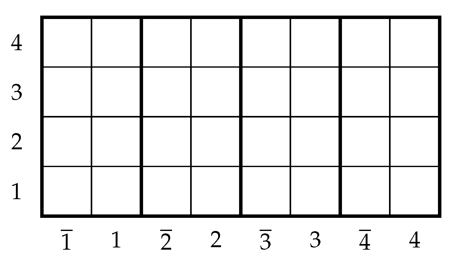
Definition 11.

Let $n\ge 1$. The type B Laguerre board of size n, denoted by ${\mathcal{L}}_n^{\left(B\right)}$, is a rectangular signed board with row set $\left[n\right]=\{1,2,\dots ,n\}$ and column set $\{\overline{1},1,\overline{2},2,\dots ,\overline{n},n\}$, grouped into opposite pairs $\{j,\overline{j}\}$ for $j\in \left[n\right]$. Equivalently, the set of cells of ${\mathcal{L}}_n^{\left(B\right)}$ consists of

$${\mathcal{L}}_n^{\left(B\right)}=\{(r,j):r\in \left[n\right],j\in {\langle n\rangle }^{\prime }\}.$$

An illustration of the type B Laguerre board ${\mathcal{L}}_4^{\left(B\right)}$ is shown in Figure 4.

We now define rook placements on the type B Laguerre board.

Definition 12.

A type B rook placement on ${\mathcal{L}}_n^{\left(B\right)}$ is a set P of cells (rooks) of ${\mathcal{L}}_n^{\left(B\right)}$ such that

1. 

(Row condition) No two rooks lie in the same row.

2. 

(Opposite-column condition) for each $j\in \left[n\right]$, at most one rook lies in the pair of opposite columns $\{j,\overline{j}\}$.

Equivalently, a type B rook placement is a non-attacking placement in which each rook occupies a distinct row and a distinct absolute column index; for a given index j, the rook may be placed in either of the two signed columns j or $\overline{j}$.

Definition 13.

Let $n\ge 1$ and $0\le k\le n$, where k denotes the number of all rows that do not contain a rook. Let ${\mathcal{L}}_n^{\left(B\right)}$ be the type B Laguerre board. An anchored rook placement of type $(n,k)$ is a type B rook placement P on ${\mathcal{L}}_n^{\left(B\right)}$ satisfying the following:

• (Cut rows) Exactly k rows contain no rook.
• (Leader columns) There exist k distinct absolute column indices $\{j_1,\dots ,j_k\}$ such that neither $j_i$ nor $\overline{j_i}$ contains a rook.

Note that every non-cut row in an anchored placement contains exactly one rook. Equivalently, an anchored placement consists of exactly $n-k$ rooks, each placed in a distinct non-cut row and a distinct absolute column index not among the leaders, with an independent choice of signed column j or $\overline{j}$ for each rook.

Remark 6.

The use of empty (cut) rows to encode the beginnings of blocks is standard in rook models for Lah numbers. We use the term anchored to indicate that the placement is determined with respect to prescribed cut rows and leader column indices.

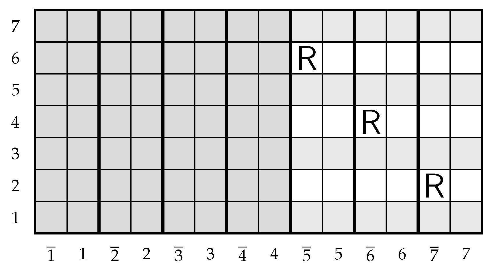
Example 8.

Let $n=4$ and $k=2$. Choose the cut rows $\{1,3\}$ and the leader columns $\{2,4\}$. The remaining rows are then $\{2,4\}$, and the available absolute column indices are $\{1,3\}$. For example, placing rooks in the cells $(2,\overline{1})$ and $(4,3)$ yields an anchored type B Laguerre rook placement of type $(4,2)$, which is illustrated in Figure 5. In this case, the leader columns $\{2,4\}$ forbid the use of the absolute indices 2 and 4, while the cut rows $\{1,3\}$ remain empty.

We now illustrate how a signed set partition gives rise to an anchored type B Laguerre rook placement. The leader indices are assigned according to the positions of the selected pairs in the ordered list.

Example 9.

Let $\pi =02\overline{2}\mid \overline{1}7/1\overline{7}\mid \overline{3}\overline{6}/36\mid \overline{4}5/4\overline{5}$ be a signed set partition. The set of absolute values appearing in π is $\{1,2,3,4,5,6,7\}$, so $n=7$. To obtain an ordered structure appropriate for the Laguerre setting, we choose the zero block together with one block from each opposite pair, preserving the given order. This results in the four ordered blocks

$$(0,2,\overline{2}),(\overline{1},7),(\overline{3},\overline{6}),(\overline{4},5),$$

and hence $k=4$. Indexing the selected pairs from left to right by $1,2,3,4$ gives the leader absolute indices $\{1,2,3,4\}$, represented by the leader columns $\{1,2,3,4\}$.

Now, we choose the cut rows $\{1,3,5,7\}$. The remaining rows are $\{2,4,6\}$, and each must contain exactly one rook. Placing the corresponding rooks in the non-cut rows yields an anchored placement. For instance, choosing the negative signed column for each rook gives the placement

$$(2,\overline{7}),(4,\overline{6}),(6,\overline{5}).$$

This defines an anchored type B Laguerre rook placement of type $(7,4)$, demonstrated in Figure 6.

Remark 7.

The use of cut rows and leader columns leads to anchored type B Laguerre rook placements, which encode block structure and naturally yield the Lah numbers of type B.

Definition 14.

Let $n\ge 1$ and $0\le k\le n$. Let ${\mathcal{R}}_{n-k}^{\left(B\right)}\left({\mathcal{L}}_n^{\left(B\right)}\right)$ denote the set of all anchored type B Laguerre rook placements of type $(n,k)$ on ${\mathcal{L}}_n^{\left(B\right)}$. The type B Laguerre rook number is

$$r_{n-k}^{\left(B\right)}\left({\mathcal{L}}_n^{\left(B\right)}\right)=\left|{\mathcal{R}}_{n-k}^{\left(B\right)}\left({\mathcal{L}}_n^{\left(B\right)}\right)\right|.$$

We now show that these rook numbers coincide with the type B Lah numbers introduced in [15]. In particular, they satisfy a type B analogue of the classical relation (5).

Theorem 3.

Let $n\ge 1$ and $0\le k\le n$. Then, the type B Laguerre rook number is

$$r_{n-k}^{\left(B\right)}\left({\mathcal{L}}_n^{\left(B\right)}\right)=L_B(n,k)={\left({\displaystyle \genfrac{}{}{0pt}{}{n}{k}}\right)}^2{2}^{n-k}(n-k)!,$$

where $L_B(n,k)$ denotes the Lah numbers of type B.

Proof. 

An anchored placement of type $(n,k)$ is determined by the following independent choices. First, choose the k cut rows in $\left({\displaystyle \genfrac{}{}{0pt}{}{n}{k}}\right)$ ways. Independently, choose the k leader absolute column indices, again in $\left({\displaystyle \genfrac{}{}{0pt}{}{n}{k}}\right)$ ways. The remaining $n-k$ rows must contain exactly one rook, and these rooks occupy the remaining $n-k$ absolute column indices bijectively, contributing $(n-k)!$ possibilities. Finally, for each rook there is an independent choice of sign, since it may be placed in either of the two signed columns j or $\overline{j}$ corresponding to its absolute index, yielding a factor of $2^{n-k}$. Multiplying these independent choices gives

$${\left({\displaystyle \genfrac{}{}{0pt}{}{n}{k}}\right)}^2{2}^{n-k}(n-k)!,$$

as claimed. □

Example 10.

We illustrate Theorem 3 in the case $n=4$ and $k=2$, using the anchored type B Laguerre rook placements described above in Example 8.

First, we choose 2 cut rows, which can be performed in $\left({\displaystyle \genfrac{}{}{0pt}{}{4}{2}}\right)=6$ ways. Independently, we select 2 leader absolute column indices, again in $\left({\displaystyle \genfrac{}{}{0pt}{}{4}{2}}\right)=6$ ways. The remaining 2 rows must each contain exactly one rook, and these rooks occupy the remaining 2 absolute column indices bijectively, contributing $2!=2$ possibilities. Finally, each rook may be placed in either of the two signed columns corresponding to its absolute index, yielding an additional factor of $2^2=4$.

Thus, the number of anchored type B Laguerre rook placements of type $(4,2)$ is

$${\left({\displaystyle \genfrac{}{}{0pt}{}{4}{2}}\right)}^2{2}^{2}2!=288,$$

which coincides with the value $L_B(4,2)$ given in Theorem 3.

It follows from the part 1 of Lemma 3.3.1 in [15] that for all $n\ge 0$ we have

$${\displaystyle {\left[x\right]}_n^B=\sum _{k=0}^n{L}_B(n,k){\left(x\right)}_k^B.}$$

(13)

Taking into account Theorem 3 and Equation (13), we deduce the following result in the sense of the Formula (3).

Corollary 1.

For all $n\ge 0$, we have

$${\displaystyle {\left[x\right]}_n^B=\sum _{k=0}^n{r}_{n-k}^{\left(B\right)}\left({\mathcal{L}}_n^{\left(B\right)}\right){\left(x\right)}_k^B.}$$

The recurrence relation of $L_B(n,k)$ is given by

$$L_B(n,k)=L_B(n-1,k-1)+2(n+k)L_B(n-1,k)$$

for all $n,k\in \mathbb{N}$ with the initial conditions $L_B(n,0)=2^{n}n!$, $L_B(n,n)=1$, and $L_B(n,k)=0$ if $k<0$ (see [15]). Therefore, we can immediately write the following recursive formula for $r_{n-k}^{\left(B\right)}\left({\mathcal{L}}_n^{\left(B\right)}\right)$:

$$r_{n-k}^{\left(B\right)}\left({\mathcal{L}}_n^{\left(B\right)}\right)=r_{n-k}^{\left(B\right)}\left({\mathcal{L}}_{n-1}^{\left(B\right)}\right)+2(n+k)r_{n-k-1}^{\left(B\right)}\left({\mathcal{L}}_{n-1}^{\left(B\right)}\right).$$

Since the exponential generating function of $L_B(n,k)$ for a fixed k is the form ${\sum }_{n\ge 0}{L}_B(n,k){\displaystyle \frac{x^n}{n!}}={\displaystyle \frac{x^k}{{(1-2x)}^{k+1}k!}}$, we obtain the exponential generating function of $r_{n-k}^{\left(B\right)}\left({\mathcal{L}}_n^{\left(B\right)}\right)$ as

$$\sum _{n\ge 0}{r}_{n-k}^{\left(B\right)}\left({\mathcal{L}}_n^{\left(B\right)}\right){\displaystyle \frac{x^n}{n!}}={\displaystyle \frac{x^k}{{(1-2x)}^{k+1}k!}}.$$

4. Conclusions

In this paper, we introduced a rook-theoretic model for signed restricted growth functions of type B by defining type B Ferrers boards equipped with the level order. Moreover, we defined natural signed and level-weighted statistics and constructed a bijection between signed restricted growth functions and type B rook placements. This correspondence gives a geometric interpretation of the statistics and yields the $(p,q)$-Stirling numbers of type B, together with their recurrence relations and generating functions. Furthermore, we introduced anchored type B Laguerre boards and rook placements and showed that they are enumerated by the type B Lah numbers.

An interesting direction for future research is to define suitable weighted statistics on anchored type B Laguerre rook placements, similar to the statistics considered in the Stirling case. Such a refinement would lead to a $(p,q)$-analogue of the Lah numbers of type B. Although $(p,q)$-analogues of the Lah numbers have been studied in [16], to the best of our knowledge a corresponding construction in the Coxeter group of type B has not yet been developed. Establishing this refinement, together with its associated recurrences and generating functions, remains open.

As a direction for future work, one may consider type D set partitions. A set partition of type D is a signed set partition of $\langle n\rangle$ whose zero block contains at least two positive elements or no positive elements of $\left[n\right]$ (see [6]). Since type D set partitions are covered by type B set partitions, $(p,q)$-Stirling numbers of type D with their recurrence relations and generating functions can be studied by employing a canonical bijection between the family of type D set partitions and a special subset of the signed restricted growth functions.