Conditional Sequence Modeling for Safe Reinforcement Learning

Abstract

Offline safe reinforcement learning (RL) aims to learn policies from a fixed dataset while maximizing performance under cumulative cost constraints. In practice, deployment requirements often vary across scenarios, necessitating a single policy capable of zero-shot adaptation to different cost thresholds. However, most existing offline safe RL methods are trained under a pre-specified threshold, yielding policies with limited generalization and deployment flexibility across cost thresholds. Motivated by recent progress in conditional sequence modeling (CSM), which enables flexible goal-conditioned control by specifying target returns, we propose Return–Cost Regularized Constrained Decision Transformer (RCDT), a CSM-based method that supports zero-shot deployment across multiple cost thresholds within a single trained policy. RCDT is the first CSM-based offline safe RL algorithm that integrates a Lagrangian-style cost penalty with an auto-adaptive penalty coefficient. To avoid overly conservative behavior and achieve a more favorable return–cost trade-off, a reward–cost-aware trajectory reweighting mechanism and Q-value regularization are further incorporated. Extensive experiments on the DSRL benchmark demonstrate that RCDT consistently improves return–cost trade-offs over representative baselines.

1. Introduction

Offline safe reinforcement learning (RL) aims to learn reliable decision-making policies from a fixed dataset while maximizing task performance under cumulative cost constraints, without any additional environment interaction [1,2,3,4]. This setting is particularly relevant for safety-critical domains such as robotics and autonomous systems, where online exploration can be prohibitively expensive and unsafe [5,6]. In practice, safety requirements vary widely; different deployment scenarios or operating conditions may impose different cost constraints, and policies often need to evaluate return–cost trade-offs and adapt across a range of cumulative cost thresholds [2,7]. Such variability highlights the need for policies with zero-shot adaptability across multiple cost thresholds [8]. However, most prior offline safe RL methods are trained under a pre-specified cost threshold, resulting in policies that are tied to that specific constraint and hence do not naturally support one-policy, zero-shot deployment across varying thresholds [9,10,11].

Recent advances in offline RL via conditional sequence modeling (CSM) suggest a promising route to accommodating varying deployment requirements within a single policy [12,13,14,15,16]. Conceptually, CSM reformulates offline RL into supervised learning on trajectory data by training a goal-conditioned action predictor [17,18]. One representative CSM approach is the Decision Transformer (DT) [17], which trains a Transformer to predict actions from trajectory prefixes conditioned on a target return-to-go (RTG) signal. At inference time, DT treats decision making as a conditional generation problem, and thus can adjust its behavior by varying the target RTG token. By making decisions directly from temporally extended trajectories, this paradigm also bypasses recursive value estimation, thereby mitigating bootstrapping errors and challenges associated with dynamic programming in offline settings [17,18]. These properties make CSM a compelling backbone candidate for offline safe RL, where one would ideally like to adapt the return–cost trade-off across budgets without retraining.

Nevertheless, a straightforward extension of DT to constrained settings, by introducing a cost-to-go (CTG) token and conditioning on both return and cost, does not necessarily yield satisfactory safety behavior. The key issue is that maximum-likelihood training encourages the model to match the conditioning signals, which obscures the asymmetry in constrained Markov decision processes (CMDPs) where return is to be optimized while cost specifies a constraint. As a result, naive CTG matching can induce unstable return–cost trade-offs and even constraint violations, especially when the dataset provides limited coverage of low-cost behaviors. Such instability and constraint violations under naive CTG-conditioned DT variants have been widely observed in prior work and in our experiments [1,3,4,7]. Consequently, a central question arises: how can we endow CSM-based policies with a principled and robust mechanism for achieving favorable return–cost trade-offs while preserving their zero-shot adaptation flexibility?

To develop a robust CSM-based approach for offline safe RL, we first analyze the discrepancy between the specified RTG/CTG signals and the resulting expected return and cumulative cost induced by a conditioned CSM policy. More precisely, we consider a fixed conditioning function $F(·)$ that determines the RTG/CTG inputs used at inference, and let $R\left(\tau \right)$ and $C\left(\tau \right)$ denote the (random) return and cumulative cost of a trajectory $\tau$ generated by the behavior policy $\beta$ from an initial state $s_1$. Our analysis shows that, under mild CMDP assumptions, this discrepancy admits an upper bound that scales as $O\left(\epsilon (\frac{1}{{\alpha }_F}+2)H^2\right)$, where ${\alpha }_F$ lower-bounds the joint return–cost coverage of the target profile in the offline dataset, i.e., $P_{{\pi }_{\beta }}\left((R\left(\tau \right),C\left(\tau \right))=F\left(s_1\right)|s_1\right)\ge {\alpha }_F$. Consequently, when the desired return–cost conditioning function $F(·)$ has low coverage (small ${\alpha }_F$), the induced optimal policy may substantially deviate from the intended RTG/CTG targets, leading to unstable return–cost trade-offs and potential constraint violations. In particular, simply specifying a high RTG together with a low CTG does not reliably yield favorable return–cost trade-offs on challenging datasets where safe high-return behaviors are under-represented. This analysis motivates augmenting naive conditioning with weighted and regularized training mechanisms that shift learning toward trajectories with better return–cost trade-offs while preserving zero-shot adaptability.

Building on this insight, we propose the first CSM-based offline safe RL algorithm that integrates a Lagrangian-style cost penalty while preserving zero-shot adaptation across different cost thresholds. We term the proposed algorithm Return–Cost Regularized Constrained Decision Transformer (RCDT). At a high level, RCDT minimizes a weighted maximum-likelihood objective augmented with an explicit cost penalty, where the penalty term is induced from a primal–dual Lagrangian formulation of CMDPs. Specifically, RCDT treats the cost-penalty coefficient as a dual variable and updates it via a standard dual-ascent step driven by the current cost estimate, which provides a principled, auto-adaptive mechanism for tuning the regularization strength while avoiding hard-wiring the policy to a single cost threshold. To avoid overly conservative behavior and achieve a more favorable return–cost trade-off, RCDT further incorporates two complementary ingredients: (i) a reward–cost-aware trajectory-level reweighting mechanism that emphasizes trajectories with desirable return–cost profiles; and (ii) Q-value regularization as an additional optimization signal to steer the policy toward high-return regions. Together, these designs decouple policy learning from any single pre-specified cost threshold while maintaining strong task performance, thereby enabling one-policy deployment across multiple cost thresholds in a zero-shot manner.

Our contributions are summarized as follows:

1.

We propose RCDT, the first CSM-based offline safe RL method that integrates a Lagrangian-style cost penalty with an auto-adaptive dual-ascent update of the penalty coefficient. RCDT achieves favorable return–cost trade-offs while enabling zero-shot deployment across multiple cost thresholds, and empirically outperforms state-of-the-art offline safe RL baselines under stringent constraints.

2.

We theoretically characterize the discrepancy between the prescribed RTG/CTG signals and the realized expected return and cumulative cost of CSM policies through the lens of joint return–cost coverage. The theoretical analysis pinpoints when a CSM policy can be regarded as a reliable backbone for offline safe RL and establishes performance limits for zero-shot control via RTG/CTG conditioning.

3.

To encourage strong return performance without inducing overly conservative behavior, we introduce a reward–cost-aware trajectory-level reweighting scheme together with Q-value regularization as complementary training signals. This design introduces an additional inductive bias toward trajectories with favorable return–cost trade-offs. Moreover, we show that the commonly used expert KL regularizer can be interpreted as a special case of our reweighting mechanism.

We evaluate RCDT on the DSRL benchmark [19] under multiple cumulative cost thresholds, where a single trained policy is assessed in a zero-shot manner across all thresholds. Experimental results show consistent improvements in return–cost trade-offs over representative baselines, establishing RCDT as a strong candidate for advancing the state-of-the-art in offline safe RL.

2. Related Work

Offline RL algorithms learn a policy entirely from a static offline dataset of past interactions, without additional access to interactions with the environment during training [13,20,21,22]. This paradigm is particularly useful when online interaction is expensive or high risk; for example, in robotic control systems and safety-critical applications.

2.1. Offline Safe Reinforcement Learning

Offline safe RL aims to learn reliable decision-making policies from a fixed dataset while maximizing task performance under cumulative cost constraints, without any additional environment interaction. Compared with standard offline RL, the central challenge is to ensure reliable constraint satisfaction under distributional shift in the state-action space, rather than merely reducing empirical costs on the training data [19].

Classical offline safe RL methods largely build on imitation learning or Lagrangian extensions of offline value-based RL algorithms. Behavior cloning (BC) treats policy learning as supervised learning on a static dataset, directly fitting the conditional action distribution given states. Safety-aware variants often introduce simple data selection or reweighting strategies that emphasize trajectories with lower cumulative cost, so that the learned policy imitates predominantly safe behaviors; however, such filtering may reduce data coverage and induce overly conservative policies [19]. Another class of approaches augments standard offline value-based RL algorithms with a Lagrangian relaxation of the CMDP constraint. Representative examples include BCQ-Lag and BEAR-Lag, which extend BCQ [23] and BEAR [24] by jointly learning reward and cost critics together with a Lagrange multiplier, and CPQ [10], which incorporates conservative regularization on both reward and cost critics to keep the learned policy close to the behavior distribution. COptiDICE [9] instead operates in the occupancy-measure space, estimating distribution corrections and solving a convex objective that maximizes return under an explicit upper bound on the expected cost.

Another line of research improves safety by explicitly reasoning about data quality and feasible regions [1,2,11,25]. LSPC [1] learns latent safety constraints using a conditional variational autoencoder and restricts policy optimization to a latent region that jointly encodes reward and cost signals, thereby mitigating out-of-distribution actions in the original state-action space. FISOR [11] revisits offline safe RL from a reachability perspective, translating hard safety constraints into the identification of the largest feasible region supported by the dataset and then solving a feasibility-dependent objective, yielding a policy that can be implemented via weighted behavior cloning with a diffusion model. TraC [2] instead recasts offline safe RL as a trajectory classification problem: it constructs desirable and undesirable trajectory sets based on cumulative rewards and costs, and optimizes a policy to imitate desirable trajectories while avoiding undesirable ones, effectively performing trajectory-level filtering. The diffusion-based offline safe RL method OASIS [25] employs a conditional diffusion model to reshape the offline action distribution toward trajectories that jointly exhibit low cost and high return, thereby suppressing unsafe behaviors that are poorly supported by the dataset.

Motivated by recent advances in large-scale sequence modeling [13,17,26], conditional sequence modeling (CSM) has emerged as a promising paradigm for offline safe RL [3,7]. Constrained Decision Transformer (CDT) [7] extends Decision Transformer by conditioning action prediction on both return-to-go (RTG) and cost-to-go (CTG) tokens, thus formulates offline safe RL as a multi-objective sequence modeling problem in which a single CSM policy can be evaluated under different cost thresholds. B2R [3] further refines how cost information is injected into the sequence model, encouraging the learned policy to respect safety boundaries while maintaining competitive returns. Compared with imitation-learning heuristics, Lagrangian extensions of value-based offline RL, and feasible-region based approaches, these CSM methods provide a particularly direct mechanism for trading off performance and safety through target conditioning, making one-policy, multi-threshold deployment more natural. Nevertheless, existing CSM-based methods largely treat RTG/CTG conditioning as a heuristic control interface, and the fundamental limits of such zero-shot adaptation remain underexplored. In this study, we analyze the discrepancy between the specified RTG/CTG signals and the resulting expected return and cumulative cost induced by a conditioned CSM policy through the lens of joint return–cost coverage, thereby characterizing when target conditioning can be reliably realized from offline data. Building on this perspective, we propose RCDT, which augments CSM training with weighted and regularized mechanisms, yielding improved return–cost trade-offs and stronger zero-shot performance over prior CSM-based offline safe RL methods.

2.2. Conditional Sequence Modeling for Offline RL

Casting RL as conditional sequence modeling has emerged as a powerful alternative to value-based and policy-gradient methods in offline settings [13,17,26,27]. Instead of explicitly estimating value functions or behavior-regularized policies, CSM methods train autoregressive models on offline trajectories and condition them on side information such as desired returns, goals, or future states [17,27,28]. This formulation enables the direct reuse of advances in sequence modeling and large-scale supervised training, while bypassing several instability sources that commonly arise in traditional offline RL, most notably the reliance on bootstrapping to propagate value estimates (one of the “deadly triad” [29]), and the myopic behaviors induced by discounting future rewards [17,30].

The most representative instantiation of this idea is the Decision Transformer (DT) [17], which conditions a causal Transformer [31] on past states, actions, and a target return, and predicts future actions so as to achieve the specified return. Subsequent studies have refined this return-conditioned formulation by modifying the conditioning signal or the learning objective. For instance, Q-learning Decision Transformer [32] and its variants replace the raw return with value-based targets obtained via dynamic programming (DP), aiming to better capture long-horizon optimality and alleviate sparse-reward issues [32,33]. Advantage-guided and return-regularized methods reshape the supervised loss using critic estimates to emphasize near-optimal actions in the offline dataset [34,35]. Similarly, Q-value Regularized Transformers (QT) [13] and Critic-Guided Decision Transformers (CGDT) [36] introduce estimated Q-values as explicit regularizers of the negative log-likelihood loss, sharpening the model’s preference for high-quality behaviors.

Another line of work employs sequence models as trajectory-level dynamics models rather than purely as policies. The Trajectory Transformer learns a joint model over sequences of states, actions, and rewards, and combines it with beam-search-style planning to generate high-return trajectories from offline data [37]. Bootstrapped variants further improve upon this idea by leveraging the learned sequence model to self-generate additional synthetic trajectories and augment the offline dataset [38]. Complementary to these data-augmentation approaches, multimodal architectures such as the Decision Transducer disentangle states, actions, and rewards into separate unimodal sequences and selectively fuse them, improving sample efficiency and representation flexibility for offline RL [39]. These approaches highlight that sequence modeling can serve as a versatile backbone for both policy learning and model-based planning in offline RL.

CSM has also been extended to safety-constrained settings by incorporating cost signals or richer specifications into the conditioning interface, enabling a single model to represent different safety–performance preferences [7,40,41]. We refer readers to Section 2.1 for a detailed discussion of representative CSM-based offline safe RL methods.

3. Preliminary

3.1. Constrained Markov Decision Process

Safe reinforcement learning can be naturally formalized as a Constrained Markov Decision Process (CMDP) [42]. A finite-horizon CMDP is defined as a tuple $(\mathcal{S},\mathcal{A},\mathcal{T},r,c,\mu ,H)$, where $\mathcal{S}$ and $\mathcal{A}$ denote the (continuous) state and action spaces. We model $(\mathcal{S},d_{\mathcal{S}})$ and $(\mathcal{A},d_{\mathcal{A}})$ as metric spaces equipped with their associated Borel $\sigma$-algebras; in standard continuous-control settings, $\mathcal{S}\subset {\mathbb{R}}^{d_s}$ and $\mathcal{A}\subset {\mathbb{R}}^{d_a}$, both equipped with Euclidean metrics. The reward function is $r:\mathcal{S}\times \mathcal{A}\to [0,1]$ and the cost function is $c:\mathcal{S}\times \mathcal{A}\to [0,1]$. The transition dynamics are defined by $\mathcal{T}$, i.e., $s_{t+1}\sim \mathcal{T}(·\mid s_t,a_t)$, and $\mu$ denotes the initial state distribution, i.e., $s_1\sim \mu$, with H being the time horizon. A trajectory is denoted by $\tau ={\left\{(s_t,a_t,r_t,c_t)\right\}}_{t=1}^H$, where $r_t$ and $c_t$ are generated according to the reward and cost functions (e.g., $r_t=r(s_t,a_t)$ and $c_t=c(s_t,a_t)$ in the deterministic case). The return and cumulative cost of $\tau$ are $R\left(\tau \right)={\sum }_{t=1}^H{r}_t$ and $C\left(\tau \right)={\sum }_{t=1}^H{c}_t$, respectively. A policy $\pi$ is considered feasible if its expected cumulative cost does not exceed a threshold $\kappa \in [0,+\infty )$, i.e., ${\mathbb{E}}_{\tau \sim \pi }\left[C\left(\tau \right)\right]\le \kappa$.

In the offline safe RL setup, algorithms are given a static dataset $\mathcal{D}$, consisting of multiple trajectories, collected by a behavior policy ${\pi }_{\beta }$. The goal of offline safe RL is to learn a feasible policy $\pi$ from $\mathcal{D}$, which maximizes the expected return while satisfying a cost constraint:

$$\arg \underset{\pi }{max}{\mathbb{E}}_{\tau \sim \pi }\left[R\left(\tau \right)\right]\mathrm{subject}\mathrm{to}{\mathbb{E}}_{\tau \sim \pi }\left[C\left(\tau \right)\right]\le \kappa .$$

(1)

3.2. Conditioned Sequence Modeling

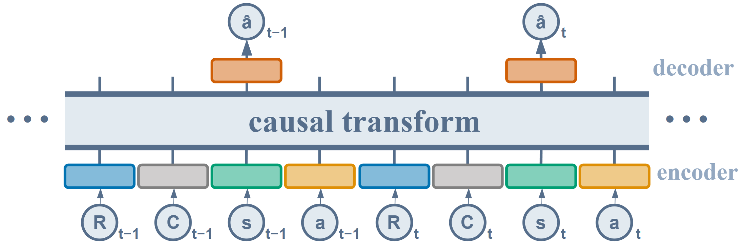
Motivated by the wide-ranging applications and remarkable success of transformer models in various domains [17,31,43,44,45,46], CSM-based methods formulate policy learning as a conditional supervised learning problem. A representative CSM approach for offline safe RL is the Constrained Decision Transformer (CDT) [7], a safety-aware extension of DT [17] in CMDP settings. The model architecture of CDT is shown in Figure 1. Specifically, during training, the policy $\pi$ is optimized by minimizing the empirical negative log-likelihood (NLL) loss over a dataset $\mathcal{D}$ of trajectories (we omit normalization here):

$${\mathcal{L}}_{\mathrm{CDT}}\left(\pi \right)=-{\sum }_{\tau \in \mathcal{D}}{\sum }_{1\le t\le H}log\pi (a_t\mid s_t,{\overline{R}}_t,{\overline{C}}_t,{\overline{\tau }}_{t-1}^K),$$

(2)

where ${\overline{R}}_t:={\sum }_{i=t}^H{r}_i$ is the return-to-go (RTG) and ${\overline{C}}_t:={\sum }_{i=t}^H{c}_i$ is the cost-to-go (CTG) for $\tau$ at time step t. ${\overline{\tau }}_{t-1}^K=({\overline{R}}_{t-K},{\overline{C}}_{t-K},s_{t-K},a_{t-K},\dots ,{\overline{R}}_{t-1},{\overline{C}}_{t-1},s_{t-1},a_{t-1})$ denotes the length-K historical context (when $t-K<1$, the context window is truncated to the available prefix of the trajectory). During inference, the model predicts a sequence of actions autoregressively conditioned on target RTG and CTG tokens.

Compared with Lagrangian extensions of value-based methods, CSM-based methods offer several advantages in the offline safe RL setting [3,7,13,36]. First, by conditioning on both RTG and CTG signals, a single CSM policy can represent a continuum of return–cost trade-offs and be evaluated under different cost thresholds without retraining [3,7]. Moreover, recasting policy learning as a supervised sequence prediction problem enables the use of stable and scalable transformer architectures that can fully exploit long-horizon dependencies and temporal structures that are critical for safe decision making [7,17].

4. Methodology

4.1. Conditioned Sequence Modeling in CMDPs

We analyze how conditional sequence modeling behaves in an idealized CMDP setting with infinite data and a fully expressive policy class. Our goal is to show that, under suitable assumptions, the policy that optimizes the CDT objective (2) is guaranteed to be near-optimal for the underlying CMDP. Let $P_{{\pi }_{\beta }}$ denote the joint distribution over states, actions, returns, and costs induced by ${\pi }_{\beta }$ and the CMDP dynamics. Recall that CDT is trained to maximize the likelihood of actions conditioned on states and target return–cost signals. Thus, when the model is given a conditioning function

$$F:\mathcal{S}\to {\mathbb{R}}^2,\mathrm{and}F\left(s\right)=\left(F_R\left(s\right),F_C\left(s\right)\right),$$

the CDT loss in (2) attempts to learn the conditional distribution $P_{{\pi }_{\beta }}(a\mid s,F\left(s\right))$. In the infinite-data and realizable limit, the optimal CDT policy (denoted by ${\pi }_F^{\mathrm{CDT}}$) for a fixed conditioning function F can be written as

$${\pi }_F^{\mathrm{CDT}}(a\mid s)=P_{{\pi }_{\beta }}\left(a\mid s,F\left(s\right)\right)={\displaystyle \frac{P_{{\pi }_{\beta }}(a\mid s)P_{{\pi }_{\beta }}\left(F\left(s\right)\mid s,a\right)}{P_{{\pi }_{\beta }}\left(F\left(s\right)\mid s\right)}}={\pi }_{\beta }(a\mid s){\displaystyle \frac{P_{{\pi }_{\beta }}\left(F\left(s\right)\mid s,a\right)}{P_{{\pi }_{\beta }}\left(F\left(s\right)\mid s\right)}}.$$

(3)

Here, $F_R\left(s\right)$ and $F_C\left(s\right)$ can be interpreted as the target RTG and CTG associated with state s, and $P_{{\pi }_{\beta }}\left(F\left(s\right)\mid s,a\right)$ denotes the probability (under ${\pi }_{\beta }$) that the trajectory starting from $(s_1=s,a_1=a)$ attains total return and cost equal to $F\left(s\right)$. In other words, ${\pi }_F^{\mathrm{CDT}}$ re-weights the behavior policy ${\pi }_{\beta }(·\mid s)$ according to how likely each action is to lead to a trajectory whose joint return–cost pair matches the conditioning signal $F\left(s\right)$.

Our analysis relies on a coverage condition and a mild regularity assumption. For an initial state $s_1\in \mathcal{S}$, let $R\left(\tau \right)$ and $C\left(\tau \right)$ denote the (random) return and cost of a trajectory $\tau$ sampled from the behavior policy ${\pi }_{\beta }$ starting from $s_1$. Represent the return–cost coverage for $s_1$ by $P_{{\pi }_{\beta }}\left((R\left(\tau \right),C\left(\tau \right))=F\left(s_1\right)|s_1\right),$ which is the conditional probability that the total return and cost of the trajectory match the conditioning signal $F\left(s_1\right)$. For any policy $\pi$, we define $J_R\left(\pi \right):={\mathbb{E}}_{\tau \sim \pi }\left[R\left(\tau \right)\right]$ and $J_C\left(\pi \right):={\mathbb{E}}_{\tau \sim \pi }\left[C\left(\tau \right)\right]$ as its expected return and expected cumulative cost, respectively.

Assumption 1. 

1. Return–cost coverage. There exists a constant ${\alpha }_F>0$ such that

$$P_{{\pi }_{\beta }}\left((R\left(\tau \right),C\left(\tau \right))=F\left(s_1\right)|s_1\right)\ge {\alpha }_F,\forall s_1\sim \mu .$$

(4)

2. 

Near determinism. (This assumption does not restrict the stochasticity of the initial state $s_1\sim \mu$.) There exist deterministic functions $T:\mathcal{S}\times \mathcal{A}\to \mathcal{S}$, $r:\mathcal{S}\times \mathcal{A}\to \mathbb{R}$, and $c:\mathcal{S}\times \mathcal{A}\to [0,1]$ such that, for all $(s,a)$ and all time steps t,

$$P\left(r_t\ne r(s,a)\mathrm{or}{c}_t\ne c(s,a)\mathrm{or}{s}_{t+1}\ne T(s,a)|s_t=s,a_t=a\right)\le \epsilon .$$

(5)

3. 

Consistency of F. For every transition $(s,a,s^{\prime })$ under the deterministic dynamics T, the conditioning function $F\left(s\right)=(F_R\left(s\right),F_C\left(s\right))$ satisfies

$$F_R\left(s\right)=F_R\left(s^{\prime }\right)+r(s,a),F_C\left(s\right)=F_C\left(s^{\prime }\right)+c(s,a).$$

(6)

Theorem 1

(Joint alignment with respect to the conditioning function in CMDPs). Consider a finite-horizon CMDP, a behavior policy ${\pi }_{\beta }$, and a conditioning function $F:\mathcal{S}\to {\mathbb{R}}^2$. Suppose Assumption 1 is satisfied. Let ${\pi }_F^{\mathrm{CDT}}$ denote the CDT policy in (3). Then there exists a universal constant $C>0$, such that

$$\begin{array}{cc}\hfill {\mathbb{E}}_{s_1\sim \mu }\left[F_R\left(s_1\right)\right]-J_R\left({\pi }_F^{\mathrm{CDT}}\right)& \le C\epsilon \left({\displaystyle \frac{1}{{\alpha }_F}}+2\right)H^2,\hfill \end{array}$$

(7)

$$\begin{array}{cc}\hfill {\mathbb{E}}_{s_1\sim \mu }\left[F_C\left(s_1\right)\right]-J_C\left({\pi }_F^{\mathrm{CDT}}\right)& \le C\epsilon \left({\displaystyle \frac{1}{{\alpha }_F}}+2\right)H^2.\hfill \end{array}$$

(8)

The proof is provided in Appendix A.1.

Theorem 1 formalizes the alignment behavior of return–cost conditioned sequence modeling in CMDPs. Under joint return–cost coverage and near-deterministic dynamics, the optimal solution to the CDT objective induced by a fixed conditioning function F produces a policy whose expected return and expected cumulative cost track the prescribed targets, with a mismatch bounded by $O\left(\epsilon (\frac{1}{{\alpha }_F}+2)H^2\right)$. This result provides a theoretical basis for viewing RTG/CTG conditioning as a mechanism for zero-shot control of the return–cost trade-off: when the target profile specified by F is sufficiently represented in the behavior data (large ${\alpha }_F$), conditioning can be realized reliably up to a controllable error. At the same time, the explicit dependence on ${\alpha }_F$ clarifies a fundamental limitation of naive target conditioning in offline safe RL. In realistic datasets where safe high-return trajectories are scarce, ${\alpha }_F$ can be small for ambitious targets, and the induced policy may substantially deviate from the intended profile, leading to unstable return–cost trade-offs and even constraint violations. In particular, simply specifying a high RTG together with a low CTG does not reliably yield favorable return–cost trade-offs on challenging datasets with limited coverage of safe, high-performance behaviors.

This motivates augmenting the plain CDT backbone with data-aware mechanisms that reshape the effective training distribution and provide additional optimization signals beyond maximum likelihood. Specifically, we seek to bias learning toward trajectories with more desirable return–cost profiles while retaining the flexibility of target conditioning for multi-threshold, zero-shot deployment. Notably, the same proof technique also extends to multi-goal conditioning by viewing each conditioning coordinate as an additional scalar, reward-like signal that obeys a Markov-consistent recursion along transitions, leading to analogous coverage-dependent alignment bounds in higher-dimensional conditioning spaces. In the following, we instantiate this principle by introducing a regularized CDT variant that incorporates trajectory-level reweighting and value-based terms, aligning with a broader line of work showing that reweighting and regularization can substantially improve DT-style and CSM-based offline RL under distribution shift and data imbalance [13,18,26,36].

Theorem 1 characterizes the infinite-data behavior of the ideal CDT policy induced by a fixed conditioning function F. We next give a finite-data extension showing that, under an additional occupancy-mismatch condition, the performance gap between the ideal CMDP-conditioned CDT policy and a finite-data estimator can be reduced to the supervised learning loss optimized by CDT. Let $d_{\beta }\left(s\right):={\displaystyle \frac{1}{H}}{\sum }_{t=1}^H{P}_{{\pi }_{\beta }}(s_t=s),$ $d_F\left(s\right):={\displaystyle \frac{1}{H}}{\sum }_{t=1}^H{P}_{{\pi }_F^{\mathrm{CDT}}}(s_t=s)$ denote the average state occupancies of the behavior policy and the ideal CDT policy, respectively. For any candidate conditional policy $\widehat{\pi }(a\mid s,R,C)$, define its deployment under the conditioning function F by ${\widehat{\pi }}_F(a\mid s):=\widehat{\pi }(a\mid s,F_R\left(s\right),F_C\left(s\right)).$ We also define the expected CDT loss as

$${\mathcal{L}}_{\mathrm{CDT}}\left(\widehat{\pi }\right):={\mathbb{E}}_{s\sim d_{\beta }}\left[{\mathbb{E}}_{(R,C)\sim P_{{\pi }_{\beta }}(·\mid s)}\left[D_{\mathrm{KL}}\left(P_{{\pi }_{\beta }}(·\mid s,R,C)\parallel \widehat{\pi }(·\mid s,R,C)\right)\right]\right].$$

(9)

Assumption 2

(Bounded occupancy mismatch). There exists a constant $C_F>0$, such that

$${\displaystyle \frac{d_F\left(s\right)}{d_{\beta }\left(s\right)}}\le C_F,\forall s\in \mathcal{S}with{d}_{\beta }\left(s\right)>0.$$

Theorem 2

(Finite-data reduction of CMDP-conditioned CDT to supervised learning). Consider the finite-horizon CMDP setting in Theorem 1, and suppose that Assumption 1 holds, i.e.,

$$P_{{\pi }_{\beta }}\left(\left(R\right(\tau ),C(\tau \left)\right)=F\left(s\right)\mid s\right)\ge {\alpha }_F,\forall s\sim \mu .$$

Assume further that Assumption 2 holds. Let $\widehat{\pi }(a\mid s,R,C)$ be any estimated conditional policy, and let ${\widehat{\pi }}_F$ denote its deployed policy under F. Then

$$\begin{array}{cc}\hfill |J_R\left({\pi }_F^{\mathrm{CDT}}\right)-J_R\left({\widehat{\pi }}_F\right)|& \le {\displaystyle \frac{C_F}{{\alpha }_F}}{H}^2\sqrt{2{\mathcal{L}}_{\mathrm{CDT}}\left(\widehat{\pi }\right)},\hfill \end{array}$$

(10)

$$\begin{array}{cc}\hfill |J_C\left({\pi }_F^{\mathrm{CDT}}\right)-J_C\left({\widehat{\pi }}_F\right)|& \le {\displaystyle \frac{C_F}{{\alpha }_F}}{H}^2\sqrt{2{\mathcal{L}}_{\mathrm{CDT}}\left(\widehat{\pi }\right)}.\hfill \end{array}$$

(11)

Proof. 

For brevity, write

$$z:=(R,C),z_F\left(s\right):=F\left(s\right)=(F_R\left(s\right),F_C\left(s\right)).$$

For each state s, define the joint distributions

$$p_s(a,z):=P_{{\pi }_{\beta }}(a,z\mid s),q_s(a,z):=P_{{\pi }_{\beta }}(z\mid s)\widehat{\pi }(a\mid s,z).$$

By construction, the ideal CDT policy satisfies

$${\pi }_F^{\mathrm{CDT}}(a\mid s)=P_{{\pi }_{\beta }}(a\mid s,z_F\left(s\right))={\displaystyle \frac{p_s(a,z_F\left(s\right))}{P_{{\pi }_{\beta }}(z_F\left(s\right)\mid s)}},$$

while

$${\widehat{\pi }}_F(a\mid s)=\widehat{\pi }(a\mid s,z_F\left(s\right))={\displaystyle \frac{q_s(a,z_F\left(s\right))}{P_{{\pi }_{\beta }}(z_F\left(s\right)\mid s)}}.$$

Therefore,

$$\begin{array}{cc}\hfill \parallel {\pi }_F^{\mathrm{CDT}}(·\mid s)-{\widehat{\pi }}_F{(·\mid s)\parallel }_1& =\sum _a\left|{\displaystyle \frac{p_s(a,z_F\left(s\right))}{P_{{\pi }_{\beta }}(z_F\left(s\right)\mid s)}}-{\displaystyle \frac{q_s(a,z_F\left(s\right))}{P_{{\pi }_{\beta }}(z_F\left(s\right)\mid s)}}\right|\hfill \\ \hfill & ={\displaystyle \frac{1}{P_{{\pi }_{\beta }}(z_F\left(s\right)\mid s)}}\sum _a|p_s(a,z_F\left(s\right))-q_s(a,z_F\left(s\right))|\hfill \\ \hfill & \le {\displaystyle \frac{1}{P_{{\pi }_{\beta }}(z_F\left(s\right)\mid s)}}\sum _{a,z}|p_s(a,z)-q_s(a,z)|.\hfill \end{array}$$

(12)

By the joint return–cost coverage assumption,

$$P_{{\pi }_{\beta }}(z_F\left(s\right)\mid s)\ge {\alpha }_F.$$

Substituting this into (12) and then applying Pinsker’s inequality gives

$$\begin{array}{cc}\hfill \parallel {\pi }_F^{\mathrm{CDT}}(·\mid s)-{\widehat{\pi }}_F{(·\mid s)\parallel }_1& \le {\displaystyle \frac{1}{{\alpha }_F}}{\parallel p_s-q_s\parallel }_1\hfill \\ \hfill & \le {\displaystyle \frac{1}{{\alpha }_F}}\sqrt{2D_{\mathrm{KL}}(p_s\parallel q_s)}.\hfill \end{array}$$

(13)

Next, we bound the performance difference by the action-distribution mismatch. For reward, by the standard performance-difference decomposition for finite-horizon MDPs,

$$\begin{array}{cc}\hfill J_R\left({\pi }_F^{\mathrm{CDT}}\right)-J_R\left({\widehat{\pi }}_F\right)& =\sum _{t=1}^H{\mathbb{E}}_{s_t\sim d_t^F}\left[\sum _a\left({\pi }_F^{\mathrm{CDT}}(a\mid s_t)-{\widehat{\pi }}_F(a\mid s_t)\right)Q_{R,t}^{{\widehat{\pi }}_F}(s_t,a)\right],\hfill \end{array}$$

(14)

where $d_t^F$ is the state distribution at time t under ${\pi }_F^{\mathrm{CDT}}$, and $Q_{R,t}^{{\widehat{\pi }}_F}$ is the reward-to-go under ${\widehat{\pi }}_F$. Since each per-step reward is bounded by 1, we have

$$\parallel Q_{R,t}^{{\widehat{\pi }}_F}{(s,·)\parallel }_{\infty }\le H-t+1\le H.$$

Hence,

$$\begin{array}{cc}\hfill |J_R\left({\pi }_F^{\mathrm{CDT}}\right)-J_R\left({\widehat{\pi }}_F\right)|& \le H\sum _{t=1}^H{\mathbb{E}}_{s_t\sim d_t^F}\left[\parallel {\pi }_F^{\mathrm{CDT}}(·\mid s_t)-{\widehat{\pi }}_F(·\mid s_t){\parallel }_1\right]\hfill \\ \hfill & =H^2{\mathbb{E}}_{s\sim d_F}\left[\parallel {\pi }_F^{\mathrm{CDT}}(·\mid s)-{\widehat{\pi }}_F{(·\mid s)\parallel }_1\right].\hfill \end{array}$$

(15)

Using Assumption 2,

$${\mathbb{E}}_{s\sim d_F}\left[g\left(s\right)\right]\le C_F{\mathbb{E}}_{s\sim d_{\beta }}\left[g\left(s\right)\right]$$

for any non-negative function g. Applying this to (15) and then using (13), we obtain

$$\begin{array}{cc}\hfill |J_R\left({\pi }_F^{\mathrm{CDT}}\right)-J_R\left({\widehat{\pi }}_F\right)|& \le C_F{H}^2{\mathbb{E}}_{s\sim d_{\beta }}\left[\parallel {\pi }_F^{\mathrm{CDT}}(·\mid s)-{\widehat{\pi }}_F{(·\mid s)\parallel }_1\right]\hfill \\ \hfill & \le {\displaystyle \frac{C_F}{{\alpha }_F}}{H}^2{\mathbb{E}}_{s\sim d_{\beta }}\left[\sqrt{2D_{\mathrm{KL}}(p_s\parallel q_s)}\right]\hfill \\ \hfill & \le {\displaystyle \frac{C_F}{{\alpha }_F}}{H}^2\sqrt{2{\mathbb{E}}_{s\sim d_{\beta }}\left[D_{\mathrm{KL}}(p_s\parallel q_s)\right]},\hfill \end{array}$$

(16)

where the last step follows from Jensen’s inequality.

It remains for us to identify the expectation in (16) with the CDT loss. Since

$$p_s(a,z)=P_{{\pi }_{\beta }}(z\mid s)P_{{\pi }_{\beta }}(a\mid s,z),q_s(a,z)=P_{{\pi }_{\beta }}(z\mid s)\widehat{\pi }(a\mid s,z),$$

the chain rule of KL divergence yields

$$\begin{array}{c}{D}_{\mathrm{KL}}(p_s\parallel q_s)={\mathbb{E}}_{z\sim P_{{\pi }_{\beta }}(·\mid s)}\left[D_{\mathrm{KL}}\left(P_{{\pi }_{\beta }}(·\mid s,z)\parallel \widehat{\pi }(·\mid s,z)\right)\right].\end{array}$$

(17)

Taking expectation over $s\sim d_{\beta }$ gives exactly ${\mathcal{L}}_{\mathrm{CDT}}\left(\widehat{\pi }\right)$ in (9). Substituting into (16) proves (10).

The proof of the cost bound is identical. Since each per-step cost is bounded by 1, we have

$$\parallel Q_{C,t}^{{\widehat{\pi }}_F}{(s,·)\parallel }_{\infty }\le (H-t+1)\le H,$$

which yields

$$|J_C\left({\pi }_F^{\mathrm{CDT}}\right)-J_C\left({\widehat{\pi }}_F\right)|\le {\displaystyle \frac{C_F}{{\alpha }_F}}{H}^2\sqrt{2{\mathcal{L}}_{\mathrm{CDT}}\left(\widehat{\pi }\right)}.$$

This completes the proof.    □

Theorem 2 reduces the CMDP performance gap to the supervised loss optimized by CDT. We next convert this reduction into a finite sample bound under a finite policy class and standard uniform-convergence assumptions.

Let $\mathcal{D}={\left\{(s_i,a_i,R_i,C_i)\right\}}_{i=1}^N$ be a dataset of N i.i.d. samples drawn from the joint distribution induced by $d_{\beta }\left(s\right)$ and $P_{{\pi }_{\beta }}(a,R,C\mid s)$. For a policy class $\mathsf{\Pi }$, define the empirical loss

$${\widehat{\mathcal{L}}}_{\mathrm{CDT}}\left(\pi \right):={\displaystyle \frac{1}{N}}\sum _{i=1}^N\left(-log\pi (a_i\mid s_i,R_i,C_i)\right),$$

(18)

and let $\widehat{\pi }\in arg{min}_{\pi \in \mathsf{\Pi }}{\widehat{\mathcal{L}}}_{\mathrm{CDT}}\left(\pi \right).$

Corollary 1

(Sample complexity of plain CMDP-conditioned CDT). Under the assumptions of Theorem 2, additionally assume that

1.

Π is finite;

2.

There exists a constant $c>0$ such that

$$0\le -log\pi (a\mid s,R,C)\le c,\forall \pi \in \mathsf{\Pi },\forall (s,a,R,C);$$

3.

The approximation error of Π is bounded by ${\epsilon }_{\mathrm{approx}}$, i.e.,

$$\underset{\pi \in \mathsf{\Pi }}{min}{\mathcal{L}}_{\mathrm{CDT}}\left(\pi \right)\le {\epsilon }_{\mathrm{approx}}.$$

Then for any $\delta \in (0,1)$, with probability at least $1-\delta$,

$$\begin{array}{cc}\hfill |J_R\left({\pi }_F^{\mathrm{CDT}}\right)-J_R\left({\widehat{\pi }}_F\right)|& \le {\displaystyle \frac{C_F}{{\alpha }_F}}{H}^2\sqrt{2{\epsilon }_{\mathrm{approx}}+4c\sqrt{{\displaystyle \frac{log\left|\mathsf{\Pi }\right|+log(2/\delta )}{2N}}}},\hfill \end{array}$$

(19)

$$\begin{array}{cc}\hfill |J_C\left({\pi }_F^{\mathrm{CDT}}\right)-J_C\left({\widehat{\pi }}_F\right)|& \le {\displaystyle \frac{C_F}{{\alpha }_F}}{H}^2\sqrt{2{\epsilon }_{\mathrm{approx}}+4c\sqrt{{\displaystyle \frac{log\left|\mathsf{\Pi }\right|+log(2/\delta )}{2N}}}}.\hfill \end{array}$$

(20)

Equivalently, up to universal constants,

$$\begin{array}{cc}\hfill |J_R\left({\pi }_F^{\mathrm{CDT}}\right)-J_R\left({\widehat{\pi }}_F\right)|& \le O\left({\displaystyle \frac{C_F}{{\alpha }_F}}{H}^2\left[\sqrt{c}{\left({\displaystyle \frac{(log|\mathsf{\Pi }|+log(1/\delta \left)\right)}{N}}\right)}^{1/4}+\sqrt{{\epsilon }_{\mathrm{approx}}}\right]\right),\hfill \end{array}$$

(21)

$$\begin{array}{cc}\hfill |J_C\left({\pi }_F^{\mathrm{CDT}}\right)-J_C\left({\widehat{\pi }}_F\right)|& \le O\left({\displaystyle \frac{C_F}{{\alpha }_F}}{H}^2\left[\sqrt{c}{\left({\displaystyle \frac{(log|\mathsf{\Pi }|+log(1/\delta \left)\right)}{N}}\right)}^{1/4}+\sqrt{{\epsilon }_{\mathrm{approx}}}\right]\right).\hfill \end{array}$$

(22)

Proof. 

For each fixed $\pi \in \mathsf{\Pi }$, the random variable

$${\ell }_{\pi }(s,a,R,C):=-log\pi (a\mid s,R,C)$$

takes values in $[0,c]$. Therefore, by Hoeffding’s inequality,

$$Pr\left(|{\widehat{\mathcal{L}}}_{\mathrm{CDT}}\left(\pi \right)-{\mathcal{L}}_{\mathrm{CDT}}\left(\pi \right)|\ge \eta \right)\le 2exp\left(-{\displaystyle \frac{2N{\eta }^2}{c^2}}\right).$$

Applying a union bound over all $\pi \in \mathsf{\Pi }$, we obtain that with probability at least $1-\delta$,

$$\underset{\pi \in \mathsf{\Pi }}{sup}|{\widehat{\mathcal{L}}}_{\mathrm{CDT}}\left(\pi \right)-{\mathcal{L}}_{\mathrm{CDT}}\left(\pi \right)|\le c\sqrt{{\displaystyle \frac{log\left|\mathsf{\Pi }\right|+log(2/\delta )}{2N}}}.$$

(23)

Let

$${\pi }_{\mathsf{\Pi }}^{★}\in arg\underset{\pi \in \mathsf{\Pi }}{min}{\mathcal{L}}_{\mathrm{CDT}}\left(\pi \right).$$

Since $\widehat{\pi }$ minimizes the empirical loss,

$${\widehat{\mathcal{L}}}_{\mathrm{CDT}}\left(\widehat{\pi }\right)\le {\widehat{\mathcal{L}}}_{\mathrm{CDT}}\left({\pi }_{\mathsf{\Pi }}^{★}\right).$$

Using (23) twice, we obtain

$$\begin{array}{cc}\hfill {\mathcal{L}}_{\mathrm{CDT}}\left(\widehat{\pi }\right)& \le {\widehat{\mathcal{L}}}_{\mathrm{CDT}}\left(\widehat{\pi }\right)+c\sqrt{{\displaystyle \frac{log\left|\mathsf{\Pi }\right|+log(2/\delta )}{2N}}}\hfill \\ \hfill & \le {\widehat{\mathcal{L}}}_{\mathrm{CDT}}\left({\pi }_{\mathsf{\Pi }}^{★}\right)+c\sqrt{{\displaystyle \frac{log\left|\mathsf{\Pi }\right|+log(2/\delta )}{2N}}}\hfill \\ \hfill & \le {\mathcal{L}}_{\mathrm{CDT}}\left({\pi }_{\mathsf{\Pi }}^{★}\right)+2c\sqrt{{\displaystyle \frac{log\left|\mathsf{\Pi }\right|+log(2/\delta )}{2N}}}\hfill \\ \hfill & \le {\epsilon }_{\mathrm{approx}}+2c\sqrt{{\displaystyle \frac{log\left|\mathsf{\Pi }\right|+log(2/\delta )}{2N}}}.\hfill \end{array}$$

(24)

Substituting (24) into Theorem 2 gives (19) and (20). The simplified $N^{-1/4}$-form follows by

$$\sqrt{x+y}\le \sqrt{x}+\sqrt{y}.$$

This completes the proof.    □

Remark 1.

Assumption 1 adopts an equality-based return–cost coverage condition,

$$P_{{\pi }_{\beta }}\left((R\left(\tau \right),C\left(\tau \right))=F\left(s_1\right)\mid s_1\right)\ge {\alpha }_F,$$

which is consistent with prior theoretical analyses of conditional sequence modeling in RL [18,26] and is particularly natural in idealized or tokenized formulations where return and cost signals are discrete or effectively quantized. The coverage condition can be extended in a straightforward manner to neighborhood-based (δ) coverage, which replaces exact matching by requiring non-trivial probability mass in a δ-neighborhood of the target signal, i.e.,

$$P_{{\pi }_{\beta }}\left(\parallel (R\left(\tau \right),C\left(\tau \right))-F\left(s_1\right)\parallel \le \delta \mid s_1\right).$$

Another closely related perspective is to define coverage through density-based support via a kernel $K_{\delta }:{\mathbb{R}}^2\to {\mathbb{R}}_{\ge 0}$ (e.g., a Gaussian kernel or a ball indicator); for example,

$${\tilde{\alpha }}_F:=\underset{s_1\sim \mu }{inf}{\mathbb{E}}_{(R,C)\sim P_{{\pi }_{\beta }}(·\mid s_1)}\left[K_{\delta }\left((R,C)-F\left(s_1\right)\right)\right].$$

In Equation (3), such a smoothing corresponds to replacing $P_{{\pi }_{\beta }}\left(F\left(s\right)\mid s,a\right)$ by a smoothed likelihood of landing near $F\left(s\right)$, yielding the same reweighting interpretation in a continuous manner.

4.2. Trajectory-Weighted Value-Regularized Constrained Decision Transformer

Building on CDT, we introduce two data-aware training ingredients to improve algorithm performance while retaining the RTG/CTG conditioning interface for multi-threshold, zero-shot deployment. Specifically, we (i) reshape the effective training distribution via trajectory-level reweighting toward more desirable return–cost profiles, and (ii) incorporate value-based guidance as an additional optimization signal to discourage overly conservative behaviors. This design follows the technical progression summarized in

Table 1. Optimization objectives for DT-based CSM methods.

Method	Optimization Objective
Offline RL
DT [17]	${\mathcal{L}}_{\mathrm{DT}}\left(\theta \right)=-{\sum }_{\tau \in \mathcal{D}}{\sum }_{1\le t\le H}log{\pi }_{\theta }\left(a_t\right|s_t,{\overline{R}}_t,{\overline{\tau }}_{t-1}^K)$
QT [13]	${\mathcal{L}}_{\mathrm{DT}}\left(\theta \right)-\eta {\mathbb{E}}_{\tau \sim \mathcal{D}}{\mathbb{E}}_{s_t\sim \tau ,a_t\sim {\pi }_{\theta }}\left[Q^{{\pi }_{\theta }}(s_t,a_t)\right]$
RDT [26]	${\mathcal{L}}_{\mathrm{DT}}\left(\theta \right)+\alpha {\mathbb{E}}_{\tau \sim {\mathcal{D}}_e}{\sum }_{i=t}^H\mathrm{KL}\left[{\pi }_{\theta }(·|s_t,{\overline{R}}_t,{\overline{\tau }}_{t-1}^K)\parallel {\pi }^e(·|s_t)\right]$
RVDT [26]	${\mathcal{L}}_{\mathrm{DT}}\left(\theta \right)-\eta {\mathbb{E}}_{\tau \sim \mathcal{D}}{\mathbb{E}}_{s_t\sim \tau ,a_t\sim {\pi }_{\theta }}\left[Q^{{\pi }_{\theta }}(s_t,a_t)\right]+\alpha {\mathbb{E}}_{\tau \sim {\mathcal{D}}_e}{\sum }_{t=1}^H\mathrm{KL}\left[{\pi }_{\theta }(·|s_t,{\overline{R}}_t,{\overline{\tau }}_{t-1}^K)\parallel {\pi }^e(·|s_t)\right]$
Offine Safe RL
CDT [7]	${\mathcal{L}}_{\mathrm{CDT}}\left(\pi \right)=-{\sum }_{\tau \in \mathcal{D}}{\sum }_{1\le t\le H}log\pi \left(a_t\right|s_t,{\overline{R}}_t,{\overline{C}}_t,{\overline{\tau }}_{t-1}^K)$
TVCDT (ours)	$-{\sum }_{\tau \in \mathcal{D}}{\sum }_{t=1}^H{W}_{\tau }log{\pi }_{\theta }\left(a_t|s_t,{\overline{R}}_t,{\overline{C}}_t,{\overline{\tau }}_{t-1}^K\right)-\eta {\mathbb{E}}_{\tau \sim \mathcal{D}}{\mathbb{E}}_{s_t\sim \tau ,a_t\sim {\pi }_{\theta }}\left[Q^{{\pi }_{\theta }}(s_t,a_t)\right]$
RCDT (ours)	$-{\sum }_{\tau \in \mathcal{D}}{\sum }_{t=1}^H{W}_{\tau }log{\pi }_{\theta }\left(a_t|s_t,{\overline{R}}_t,{\overline{C}}_t,{\overline{\tau }}_{t-1}^K\right)-\eta {\mathbb{E}}_{\tau \sim \mathcal{D}}{\mathbb{E}}_{s_t\sim \tau ,a_t\sim {\pi }_{\theta }}\left[Q^{{\pi }_{\theta }}(s_t,a_t)\right]+\lambda {\mathbb{E}}_{s_t\sim \tau ,a_t\sim {\pi }_{\theta }}\left[C^{{\pi }_{\theta }}(s_t,a_t)\right]$

: it generalizes the sub-dataset resampling used in DT-style methods (e.g., RDT/RVDT) to a more flexible trajectory-level scheme, and adapts the Q-value regularization principle of QT to the constrained CDT setting.

Let $R\left(\tau \right)$ and $C\left(\tau \right)$ denote the cumulative return and cumulative cost of a trajectory $\tau \in \mathcal{D}$ respectively. We introduce a non-negative weighting function

$$\mathcal{W}:{\mathbb{R}}^2\to {\mathbb{R}}_{>0},W_{\tau }=\mathcal{W}\left(R\left(\tau \right),C\left(\tau \right)\right),$$

(25)

which assigns larger weights to trajectories that exhibit more favorable return–cost trade-offs. It suffices to note that $W_{\tau }$ depends jointly on return and cost, and therefore encodes both performance and safety preferences at the trajectory level. Given these weights, consider the following weighted variant of the CDT loss:

$$\mathcal{L}\left(\theta \right)=-\sum _{\tau \in \mathcal{D}}\sum _{t=1}^H{W}_{\tau }log{\pi }_{\theta }\left(a_t|s_t,{\overline{R}}_t,{\overline{C}}_t,{\overline{\tau }}_{t-1}^K\right).$$

(26)

The loss (26) preserves the behavior-cloning structure of CDT while explicitly rebalancing the empirical training distribution toward trajectories that are simultaneously high-return and low-cost.

To connect this formulation with existing DT-based methods, we draw a connection to the KL-based expert regularization used by RDT and RVDT in prior work [26]. Consider the RDT objective:

$${\mathcal{L}}_{\mathrm{RDT}}\left(\theta \right)={\mathbb{E}}_{\tau \sim \mathcal{D}}\left[\sum _{t=1}^H-log{\pi }_{\theta }\left(a_t|s_t,g\left({\tau }_t\right),{\overline{\tau }}_{t-1}^K\right)\right]+\alpha {\mathbb{E}}_{\tau \sim {\mathcal{D}}_e}\left[\sum _{t=1}^H\mathrm{KL}\left({\pi }_{\theta }(·|s_t,g\left({\tau }_t\right),{\overline{\tau }}_{t-1}^K)\parallel {\pi }^e(·|s_t)\right)\right],$$

(27)

where ${\mathcal{D}}_e\subset \mathcal{D}$ is a subset of near-optimal trajectories and ${\pi }^e$ is an expert policy obtained from imitation learning on ${\mathcal{D}}_e$. The following result shows that the expert KL term implicitly induces a particular trajectory-level weighting scheme, and can therefore be seen as a special case of our general reweighting formulation.

Proposition 1

(KL regularization as a special case of trajectory weighting). Assume that ${\pi }_{\theta }$ is parameterized as a factorized Gaussian policy with a fixed standard deviation and that ${\pi }^e$ is fitted on ${\mathcal{D}}_e$ via maximum-likelihood imitation learning. Then the RDT objective in Equation (27) can be rewritten as a weighted DT loss:

$$arg\underset{{\pi }_{\theta }}{min}{\mathcal{L}}_{\mathrm{RDT}}\left(\theta \right)=arg\underset{{\pi }_{\theta }}{min}{\mathbb{E}}_{\tau \sim \mathcal{D}}\left[W_{\tau }^{\mathrm{RDT}}\sum _{t=1}^H-log{\pi }_{\theta }\left(a_t|s_t,g\left({\tau }_t\right),{\overline{\tau }}_{t-1}^K\right)\right],$$

(28)

with trajectory weights $W_{\tau }^{\mathrm{RDT}}=1+\alpha \mathbb{I}\left[\tau \in {\mathcal{D}}_e\right],\alpha \ge 0.$

The proof is provided in Appendix A.2.

Proposition 1 indicates that KL-based expert regularization effectively performs a weighted resampling of expert trajectories, where all trajectories in ${\mathcal{D}}_e$ share an increased weight and all others retain unit weight. In this sense, RDT is a special case of trajectory-level reweighting that is typically constructed based on return ranking. Our formulation in Equation (26) generalizes this mechanism by allowing $W_{\tau }$ to depend on both return and cost, and by instantiating it on the constrained CDT backbone.

In addition, prior results from QT [13] and RVDT [26] indicate that value-based regularization can improve the robustness of DT-style policies for challenging offline datasets. Accordingly, we augment Equation (26) with a value guidance term and obtain

$${\mathcal{L}}_{\mathrm{TVCDT}}\left(\theta \right)=-\sum _{\tau \in \mathcal{D}}\sum _{t=1}^H{W}_{\tau }log{\pi }_{\theta }\left(a_t|s_t,{\overline{R}}_t,{\overline{C}}_t,{\overline{\tau }}_{t-1}^K\right)-\eta {\mathbb{E}}_{\tau \sim \mathcal{D}}{\mathbb{E}}_{s_t\sim \tau ,a_t\sim {\pi }_{\theta }}\left[Q^{{\pi }_{\theta }}(s_t,a_t)\right],$$

(29)

where $\eta >0$ is a regularization coefficient and $Q^{{\pi }_{\theta }}$ denotes the action-value function of the current CSM policy ${\pi }_{\theta }$. We term the resulting algorithm as Trajectory-Weighted Value-Regularized Constrained Decision Transformer (TVCDT). The first term in Equation (29) performs explicit trajectory-level return-cost reweighting on CDT, and the second term provides an optimization signal that encourages actions with higher long-term value under ${\pi }_{\theta }$.

4.3. Return–Cost Regularized Constrained Decision Transformer

While TVCDT already biases learning toward trajectories that are both high-return and low-cost, it lacks an explicit cost-penalization mechanism to further discourage unsafe behavior. A standard approach in safe reinforcement learning is to formulate policy learning as a constrained optimization problem in CMDPs and to introduce Lagrangian penalties to balance performance and safety. Following this perspective, we derive a cost-penalized training objective together with an adaptive update rule for its coefficient, while avoiding coupling CDT to a single fixed-cost threshold. To motivate the penalty term, consider minimizing the weighted CDT loss with value guidance subject to an upper bound $\kappa$ on the expected cumulative cost of the learned policy. A CMDP-style formulation can be written as

$$\begin{array}{cc}\hfill \underset{\theta }{min}& -{\sum }_{\tau \in \mathcal{D}}{\sum }_{t=1}^H{W}_{\tau }log{\pi }_{\theta }\left(a_t\mid s_t,{\overline{R}}_t,{\overline{C}}_t,{\overline{\tau }}_{t-1}^K\right)-\eta {\mathbb{E}}_{\tau \sim \mathcal{D}}{\mathbb{E}}_{s_t\sim \tau ,a_t\sim {\pi }_{\theta }}\left[Q^{{\pi }_{\theta }}(s_t,a_t)\right]\hfill \\ \hfill \mathrm{s}.\mathrm{t}.& J_c\left(\theta \right):={\mathbb{E}}_{\tau \sim \mathcal{D}}{\mathbb{E}}_{s_t\sim \tau ,a_t\sim {\pi }_{\theta }}\left[C^{{\pi }_{\theta }}(s_t,a_t)\right]\le \kappa ,\hfill \end{array}$$

(30)

where $\kappa >0$ denotes a target cost level. Introducing a Lagrange multiplier $\lambda \ge 0$ leads to the Lagrangian

$$\begin{array}{cc}\hfill {\mathcal{L}}_{\mathrm{lag}}(\theta ,\lambda )& =-{\sum }_{\tau \in \mathcal{D}}{\sum }_{t=1}^H{W}_{\tau }log{\pi }_{\theta }\left(a_t\mid s_t,{\overline{R}}_t,{\overline{C}}_t,{\overline{\tau }}_{t-1}^K\right)-\eta {\mathbb{E}}_{\tau \sim \mathcal{D}}{\mathbb{E}}_{s_t\sim \tau ,a_t\sim {\pi }_{\theta }}\left[Q^{{\pi }_{\theta }}(s_t,a_t)\right]\hfill \\ \hfill & +\lambda \left({\mathbb{E}}_{\tau \sim \mathcal{D}}{\mathbb{E}}_{s_t\sim \tau ,a_t\sim {\pi }_{\theta }}\left[C^{{\pi }_{\theta }}(s_t,a_t)\right]-\kappa \right).\hfill \end{array}$$

(31)

Equation (31) serves as a motivating formulation rather than as a strict optimization problem: it suggests that a natural way to bias the policy towards safer behaviors is to augment the training loss with the expected cost term, weighted by an appropriate coefficient. Imposing this constraint as a hard requirement tied to a fixed $\kappa$ would also be at odds with the zero-shot adaptation capability of conditional sequence modeling, where a single CDT policy is expected to generalize across a range of cost thresholds. Instead, we treat the cost term as a flexible regularizer whose influence is controlled by an adaptive coefficient $\lambda$.

Finally, we arrive at our offline safe RL algorithm, referred to as Return–Cost Regularized Constrained Decision Transformer (RCDT), by optimizing the following cost-penalized actor objective:

$$\begin{array}{cc}\hfill {\mathcal{L}}_{\mathrm{RCDT}}\left(\theta \right)& =-{\sum }_{\tau \in \mathcal{D}}{\sum }_{t=1}^H{W}_{\tau }log{\pi }_{\theta }\left(a_t\mid s_t,{\overline{R}}_t,{\overline{C}}_t,{\overline{\tau }}_{t-1}^K\right)-\eta {\mathbb{E}}_{\tau \sim \mathcal{D}}{\mathbb{E}}_{s_t\sim \tau ,a_t\sim {\pi }_{\theta }}\left[Q^{{\pi }_{\theta }}(s_t,a_t)\right]\hfill \\ \hfill & +\lambda {\mathbb{E}}_{\tau \sim \mathcal{D}}{\mathbb{E}}_{s_t\sim \tau ,a_t\sim {\pi }_{\theta }}\left[C^{{\pi }_{\theta }}(s_t,a_t)\right],\hfill \end{array}$$

(32)

where we reinterpret $\lambda >0$ as an adaptive regularization coefficient rather than an exact Lagrange multiplier associated with a fixed hard constraint, thereby using it to balance performance and safety. To obtain such an adaptive update rule, we note that the derivative of the Lagrangian in Equation (31) with respect to $\lambda$ is proportional to $J_c\left(\theta \right)-\kappa$. This suggests adjusting $\lambda$ according to whether the current policy is above or below the target cost level. In practice, let ${\widehat{J}}_c\left(\theta \right)$ denote a minibatch estimate of

$$J_c\left(\theta \right)={\mathbb{E}}_{\tau \sim \mathcal{D}}{\mathbb{E}}_{s_t\sim \tau ,a_t\sim {\pi }_{\theta }}\left[C^{{\pi }_{\theta }}(s_t,a_t)\right].$$

We update $\lambda$ using

$$\lambda \leftarrow {\mathsf{\Pi }}_{[0,{\lambda }_{max}]}\left(\lambda +\beta \left({\widehat{J}}_c\left(\theta \right)-\kappa \right)\right),$$

(33)

where ${\mathsf{\Pi }}_{[0,{\lambda }_{max}]}$ denotes the Euclidean projection onto the interval $[0,{\lambda }_{max}]$, ${\beta }_t>0$ is the update step size, ${\widehat{J}}_c\left({\theta }_t\right)$ is the estimated cumulative cost at iteration t, and $\kappa$ is the reference cost threshold. When the estimated expected cost ${\widehat{J}}_c\left(\theta \right)$ exceeds $\kappa$, $\lambda$ is increased and the cost penalty in Equation (32) becomes stronger; when the ${\widehat{J}}_c\left(\theta \right)$ falls below $\kappa$, the penalty is gradually relaxed. This update follows the primal–dual intuition of adjusting a penalty coefficient based on the current level of constraint violation, and provides an automatic way to tune the strength of safety regularization during training. Importantly, since the CDT architecture explicitly conditions on cost tokens, the resulting policy remains compatible with evaluation under multiple cost thresholds without retraining and $\kappa$ should be interpreted as a training-time reference level, rather than a hard constraint that fixes a single deployment threshold.

To further clarify the role of the adaptive coefficient $\lambda$, we note that the clipped update used in practice can be equivalently viewed as a projection step onto a compact interval. This observation does not by itself imply convergence of the full nonconvex Transformer training objective, but it does provide a simple and rigorous boundedness guarantee for the dual coefficient throughout training.

Proposition 2

(Boundedness of the adaptive coefficient). Consider the update

$${\lambda }_{t+1}={\mathsf{\Pi }}_{[0,{\lambda }_{max}]}\left({\lambda }_t+{\beta }_t\left({\widehat{J}}_c\left({\theta }_t\right)-\kappa \right)\right),$$

where ${\mathsf{\Pi }}_{[0,{\lambda }_{max}]}$ denotes the Euclidean projection onto the interval $[0,{\lambda }_{max}]$, ${\beta }_t>0$ is the update step size, ${\widehat{J}}_c\left({\theta }_t\right)$ is the estimated cumulative cost at iteration t, and κ is the reference cost threshold. Then, for any initialization ${\lambda }_0\in [0,{\lambda }_{max}]$, the iterate sequence satisfies

$${\lambda }_t\in [0,{\lambda }_{max}],\forall t\ge 0.$$

Proof. 

The result follows directly from the definition of the projection. Assume ${\lambda }_t\in [0,{\lambda }_{max}]$. Let

$$u_t:={\lambda }_t+{\beta }_t\left({\widehat{J}}_c\left({\theta }_t\right)-\kappa \right).$$

By definition of the Euclidean projection onto the closed interval $[0,{\lambda }_{max}]$,

$${\lambda }_{t+1}={\mathsf{\Pi }}_{[0,{\lambda }_{max}]}\left(u_t\right)\in [0,{\lambda }_{max}].$$

Since ${\lambda }_0\in [0,{\lambda }_{max}]$, the claim follows by induction.    □

Proposition 2 shows that the clipped update of $\lambda$ admits a standard projection-based interpretation. Therefore, the adaptive coefficient remains bounded throughout training by construction. We emphasize that this boundedness result is a property of the projected dual update itself, and should be understood as a stability guarantee for the coefficient $\lambda$, rather than as a convergence guarantee for the full nonconvex optimization of the Transformer-based objective.

In practice, the trajectory weights $W_{\tau }$ in Equation (32) are instantiated by a return–cost shaped function that increases with return and decreases with cost relative to a prescribed limit. Specifically, we use

$$W_{\tau }=exp\left(\alpha R\left(\tau \right)\right)sigmoid\left(\gamma (c_{\lim }-C\left(\tau \right))\right),$$

(34)

where $\alpha$ and $\gamma$ control the sensitivity of $W_{\tau }$ to return and cost, and $c_{\lim }$ denotes a trajectory-level cost reference. This choice is consistent with the general form $W_{\tau }=\mathcal{W}\left(R\left(\tau \right),C\left(\tau \right)\right)$ introduced in Section 4.2, and makes explicit how return and cost jointly shape the effective training distribution.

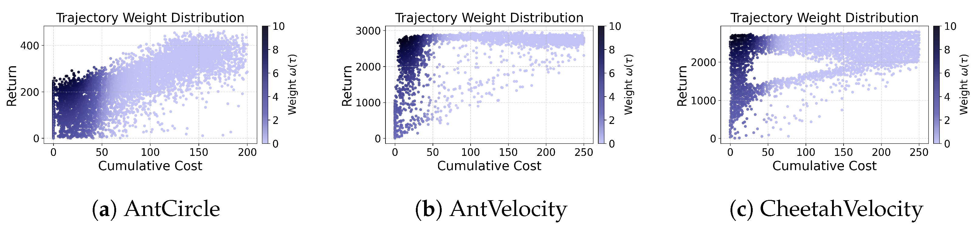
Figure 2 illustrates the effect of Equation (34) on representative tasks. Each point corresponds to a trajectory in the offline dataset, with cumulative cost on the horizontal axis and return on the vertical axis; color intensity indicates the magnitude of $W_{\tau }$ (darker means larger weight). As costs increase beyond the reference $c_{\lim }$, trajectories are progressively down-weighted, whereas trajectories that achieve higher returns while remaining within (or near) the cost reference are emphasized. This visualization highlights how trajectory-level return–cost reweighting reshapes the training signal toward safer and more performant regions of the offline data.

Putting these components together, RCDT can be viewed as a CMDP-inspired extension of CDT within the CSM paradigm. It retains the target-conditioning interface of CDT for multi-threshold, zero-shot evaluation, while augmenting maximum-likelihood training with three complementary ingredients: trajectory-level return–cost reweighting to emphasize favorable behaviors in the offline data, value-based guidance to refine the policy beyond pure imitation, and an explicit cost penalty whose coefficient is adaptively tuned to control safety in expectation. In this way, RCDT aligns with the DT-based objective design path summarized in Table 1, while remaining directly applicable to zero-shot adaptation across multiple cost thresholds at evaluation time.

4.4. Training and Inference

We instantiate RCDT using a transformer-based architecture. The policy ${\pi }_{\theta }$ is implemented as an autoregressive Transformer that takes as input a context window of past states, actions, and target return–cost tokens, and outputs the parameters of a stochastic policy. Following common practice in sequence-modeling RL, ${\pi }_{\theta }$ is modeled as a factorized Gaussian distribution whose mean and log-variance are predicted by separate fully connected output heads at each step of the sequence. For a CDT policy ${\pi }_{\theta }\left(·\mid s_i,{\overline{R}}_i,{\overline{C}}_i,{\overline{\tau }}_{i-1}^K\right)$ at timestep i, ${\overline{R}}_i$ and ${\overline{C}}_i$ denote the RTG and CTG tokens obtained by cumulatively summing future rewards and costs along the underlying trajectory, and ${\overline{\tau }}_{i-1}^K$ denotes the length-K history of past states and actions. When $i-K<1$, the context window ${\overline{\tau }}_{i-1}^K$ is truncated to the available prefix of the trajectory.

Training. The overall training pipeline of RCDT is summarized in Algorithm 1. Prior to training, the cumulative return $R\left(\tau \right)$ and cumulative cost $C\left(\tau \right)$ are computed for each trajectory $\tau \in \mathcal{D}$. These statistics are used to instantiate the trajectory weights $W_{\tau }$ via Equation (34), which increase with return and decrease with cost relative to a reference limit $c_{\lim }$. During each training iteration, a trajectory $\tau$ is sampled from the dataset, a length-K subsequence is extracted, and the corresponding CDT inputs are $(s_i,{\overline{R}}_i,{\overline{C}}_i,{\overline{\tau }}_{i-1}^K)$.

Value learning is carried out using standard offline temporal-difference (TD) methods. The reward critic $Q_{\psi }$ approximates the action-value function $Q^{{\pi }_{\theta }}$, while the cost critic $C_{\xi }$ approximates the cost-to-go function $C^{{\pi }_{\theta }}$. Given a transition $(s_{K-1},a_{K-1},r_{K-1},c_{K-1},s_K)$ from the sampled subsequence, a next action ${\widehat{a}}_K$ is drawn from the current policy ${\pi }_{\theta }(·\mid s_K,{\overline{R}}_K,{\overline{C}}_K,{\overline{\tau }}_{K-1}^K)$, and TD targets are constructed using $(s_{K-1},a_{K-1},r_{K-1},s_K,{\widehat{a}}_K)$ and $(s_{K-1},a_{K-1},c_{K-1},s_K,{\widehat{a}}_K)$ for the reward and cost critics, respectively. In practice, standard stabilization techniques such as target networks [47] and double Q-learning [48] are employed for both $Q_{\psi }$ and $C_{\xi }$.

Algorithm 1: RCDT: Return–Cost Regularized Constrained Decision Transformer

The policy parameters $\theta$ are updated by minimizing the actor loss in Equation (32). Concretely, for each CDT input in the subsequence, an action ${\widehat{a}}_i$ is sampled from ${\pi }_{\theta }(·\mid s_i,{\overline{R}}_i,{\overline{C}}_i,{\overline{\tau }}_{i-1}^K)$, and the corresponding critic evaluations $Q_{\psi }(s_i,{\widehat{a}}_i)$ and $C_{\xi }(s_i,{\widehat{a}}_i)$ are used to form a Monte Carlo estimate of the expectations in Equation (32). The trajectory weight $W_{\tau }$ is applied to the negative log-likelihood term to realise the return-cost reweighting effect. The critic-based terms provide value and cost guidance, and the combined stochastic gradient is used to update $\theta$ via gradient descent.

The coefficient $\lambda$ that controls the strength of the cost penalty is updated adaptively according to Equation (33). At each iteration, an empirical estimate ${\widehat{J}}_c\left(\theta \right)$ of $J_c\left(\theta \right)={\mathbb{E}}_{\tau \sim \mathcal{D}}{\mathbb{E}}_{s_t\sim \tau ,a_t\sim {\pi }_{\theta }}\left[C^{{\pi }_{\theta }}(s_t,a_t)\right]$ is obtained by averaging $C_{\xi }(s_i,{\widehat{a}}_i)$ over the sampled subsequence. The update $\lambda \leftarrow {[\lambda +\beta ({\widehat{J}}_c\left(\theta \right)-\kappa )]}_{+}$ then increases $\lambda$ when the current policy exceeds the reference cost level $\kappa$, and decreases it otherwise. As discussed in Section 4.3, $\lambda$ is therefore interpreted as an adaptive regularization coefficient rather than an exact Lagrange multiplier, and its update rule is inspired by Lagrangian dual ascent in safe RL.

Inference. The inference procedure of RCDT closely follows that of CDT and other CSM methods, with the additional capability of conditioning on cost. At each decision step, the model receives four input sequences: the target RTG, the target CTG, the past states, and the past actions. Given these inputs, the Transformer autoregressively predicts a sequence of K actions, of which only the final action in the window is executed in the environment.

After executing the selected action and observing the realized reward and cost, both the RTG and CTG tokens are updated for the next timestep. Specifically, the target RTG is decreased by the observed reward, and the target CTG is decreased by the observed cost, mirroring the cumulative structure used to construct ${\overline{R}}_t$ and ${\overline{C}}_t$ in the offline dataset. These updated tokens are appended to the conditioning sequence and fed back into the Transformer to generate the next action sequence. Different evaluation thresholds on the cumulative cost are imposed by choosing different initial CTG values without retraining the model. In this way, RCDT preserves the zero-shot adaptation capability of CDT across a range of safety requirements, while leveraging trajectory-level reweighting, value guidance, and cost regularization to produce policies that are both high-performing and safety-aware.

5. Experiments

We conduct a comprehensive empirical evaluation of RCDT on the DSRL benchmark [19]. In Section 5.1, we compare RCDT against a broad range of representative offline safe RL baselines spanning multiple methodological paradigms, including imitation learning [1], value-based methods [10,23,24], CSM-based approaches [7], distribution-matching methods [9], as well as data-quality and feasible-region methods [2,11]. In Section 5.2, ablation studies are conducted to analyze how each key component of RCDT affects the safety–performance trade-off, focusing on the Lagrangian-style cost penalty, trajectory-level reweighting, and Q-value regularization. Moreover, to further assess the robustness of RCDT  under more demanding evaluation settings, dataset variants from the original DSRL benchmark with (i) a lower proportion of expert-level trajectories and (ii) more imbalanced data distributions are considered.

Tasks. We evaluate RCDT on the DSRL benchmark [19], a public benchmark that includes a variety of continuous-control and robot locomotion tasks commonly used in prior offline safe RL research [1,2,4,10,11,25,49]. DSRL provides offline datasets collected from three widely used safety-critical simulators, including Mujoco-based SafetyGym [50], PyBullet-based BulletSafetyGym [51], and the autonomous-driving simulator MetaDrive [52]. In SafetyGym, we consider goal-reaching, pushing, and circle-tracking tasks with two agent morphologies (Point and Car). The agent is rewarded for completing the intended objective, such as reaching a target location, pushing an object to a goal, or tracking a circular route, while safety cost is incurred when the agent enters hazardous regions and, for circle-style tasks, when it violates the safety boundary constraints. We additionally include velocity-constrained locomotion tasks with standard Mujoco agents, including Swimmer, Hopper, HalfChee, Walker2d, and Ant. In these tasks, reward encourages forward progress, whereas cost is triggered when the agent’s speed exceeds a predefined limit. BulletSafetyGym provides analogous safety-critical locomotion tasks with different robot morphologies. We evaluate on Run and Circle tasks with multiple robots (Ball, Car, Drone, and Ant). In Run, the agent is rewarded for fast forward motion within boundaries, but incurs cost when leaving the corridor or exceeding a velocity cap. In Circle, the agent is rewarded for clockwise circular motion while being penalized for leaving a designated safe region. Finally, in MetaDrive we evaluate offline safe driving datasets with increasing scenario difficulty and traffic density (e.g., Easy/Medium/Hard combined with Sparse/Mean/Dense), which capture realistic safety–performance tensions in interactive driving. Here reward encourages route progress and stable driving, while safety cost is issued for events such as collisions and driving out of the road. Across all suites, reward promotes task completion, whereas cost penalizes safety violations. This inherent reward–cost conflict makes it necessary to balance return maximization against cumulative cost constraints: aggressively pursuing high reward can lead to constraint violations, while overly conservative policies tend to satisfy constraints at the expense of performance.

Baselines. We compare RCDT against the following baselines. (i) Imitation learning: Behavior cloning (BC) and its safety-aware variant BC-Safe [1]. (ii) Value-based with constraint handling: CPQ [10], BCQ-Lag, and BEAR-Lag, where the latter two are safety-constrained variants of BCQ [23] and BEAR [24] obtained by incorporating Lagrangian penalties. (iii) CSM-based: Constrained Decision Transformer (CDT) [7], a representative CSM method that learns conditioned policies. (iv) Distribution matching: COptiDICE [9], which performs constrained policy optimization via occupancy-measure matching in the DICE family [53]. (v) Data-quality and feasible-region methods: TraC [2], and FISOR [11], which explicitly reason about safe regions or trajectory-level feasibility.

Implementation. Our implementation of RCDT is built upon the CDT implementation provided in the OSRL (https://github.com/liuzuxin/OSRL/tree/main (accessed on 12 March 2026)) project repository released by the CDT authors. We reproduce CDT using this codebase and its recommended hyperparameters. For the remaining baselines, we either run their publicly available implementations or report results from the original papers or representative prior work [1,2,3,4], depending on availability. Additional implementation details are provided in Appendix B.2.

Evaluation. We follow the standard constraint-variation evaluation protocol for offline safe RL [1,2,19], which assesses an algorithm’s robustness and versatility under different levels of safety constraints. Concretely, each method is evaluated on every dataset under three target cumulative-cost thresholds, i.e., $\{20,40,80\}$ for SafetyGym, $\{10,20,40\}$ for BulletSafetyGym, and $\{10,20,40\}$ for MetaDrive, and the final score is obtained by averaging over these thresholds. For methods that can be evaluated under multiple thresholds without retraining (BC, BC-Safe, CDT, and our RCDT), we train a single policy per dataset and evaluate its behavior across all thresholds in a zero-shot manner. Notably, although CDT and RCDT involve a target cost level $\kappa$ during training, which is set as a fixed hyperparameter for each dataset, the learned policies remain CTG-conditioned and are evaluated across all target thresholds without additional retraining. By contrast, for threshold-dependent baselines whose training objective explicitly depends on the target constraint level, including BCQ-Lag, BEAR-Lag, COptiDICE, CPQ, FISOR, and TraC, we train separate models for different thresholds following their original training pipelines and the benchmark protocol to align with their intended training settings. Overall, this protocol provides a comprehensive assessment of the return–cost trade-off across a range of cost requirements, and it also directly validates the zero-shot deployment capability of RCDT under varying cost thresholds.

Metrics. We report the normalized return and cumulative cost as the comparison metrics, consistent with prior offline safe RL literature [1,2,19]. Let $R_{max}\left(\mathcal{T}\right)$ and $R_{min}\left(\mathcal{T}\right)$ denote the maximum and minimum returns, respectively, observed in dataset $\mathcal{T}$. The normalized return is computed by

$$R_{\mathrm{normalized}}={\displaystyle \frac{R_{\pi }-R_{min}\left(\mathcal{T}\right)}{R_{max}\left(\mathcal{T}\right)-R_{min}\left(\mathcal{T}\right)}},$$

where $R_{\pi }$ denotes the evaluated return of policy $\pi$. The normalized cumulative cost is defined by the ratio of the evaluated cumulative cost $C_{\pi }$ to the target threshold $\zeta$, i.e., $C_{\mathrm{normalized}}=C_{\pi }/\zeta$ with $\zeta >0$, noting that all costs in our setting are non-negative.

5.1. Main Results for RCDT on DSRL Benchmark

The experimental results of RCDT and all baselines on the DSRL benchmark are summarized in

Table 2. Performance comparison across DSRL tasks. For each task, RCDT reports the averaged normalized returns over three cost thresholds and 5 random seeds. Bold: Safe agents with averaged cost $<1$. Blue: Safe agents with the highest returns. ↑ means the higher the better. ↓ means the lower the better.

Task	BC-ALL		BCQ-Lag		BEAR-Lag		COptiDICE		BC-Safe		CPQ		FISOR		CDT		TraC		RCDT
	Ret↑	Cost↓	Ret↑	Cost↓	Ret↑	Cost↓	Ret↑	Cost↓	Ret↑	Cost↓	Ret↑	Cost↓	Ret↑	Cost↓	Ret↑	Cost↓	Ret↑	Cost↓	Ret↑	Cost↓
PointCircle1	0.79	3.98	0.54	2.38	0.73	3.28	0.86	5.51	0.41	0.16	0.43	0.75	0.43	14.93	0.57	0.67	0.5	0.07	0.58	0.56
PointCircle2	0.66	4.17	0.66	2.60	0.63	4.27	0.85	8.61	0.48	0.99	0.24	3.58	0.76	18.02	0.61	0.85	0.61	0.86	0.63	0.99
PointGoal1	0.65	0.95	0.71	0.98	0.74	1.18	0.49	1.66	0.43	0.54	0.57	0.35	0.64	5.38	0.62	0.78	0.44	0.36	0.68	0.79
PointGoal2	0.54	1.97	0.67	3.18	0.67	3.11	0.38	1.92	0.29	0.78	0.40	1.31	0.31	1.67	0.54	2.01	0.31	0.59	0.61	1.78
PointPush1	0.19	0.61	0.33	0.86	0.22	0.79	0.13	0.83	0.13	0.43	0.20	0.83	0.26	0.09	0.28	1.11	0.15	0.42	0.33	0.95
PointPush2	0.18	0.91	0.23	0.99	0.16	0.89	0.02	1.18	0.11	0.80	0.11	1.04	0.24	0.34	0.23	1.69	0.15	0.8	0.24	0.99
CarCircle1	0.72	4.39	0.73	5.25	0.76	5.46	0.70	5.72	0.37	1.38	0.02	2.29	0.69	10.52	0.49	1.78	0.52	1.85	0.57	2.14
CarCircle2	0.76	6.44	0.72	6.58	0.74	6.28	0.77	7.99	0.54	3.38	0.44	2.69	0.63	12.78	0.61	3.45	0.59	2.33	0.62	2.46
CarGoal1	0.39	0.33	0.47	0.78	0.61	1.13	0.35	0.54	0.24	0.28	0.79	1.42	0.49	0.12	0.59	1.01	0.38	0.39	0.61	0.99
CarGoal2	0.23	1.05	0.3	1.44	0.28	1.01	0.25	0.91	0.14	0.51	0.65	3.75	0.06	0.05	0.44	1.61	0.19	0.52	0.48	1.62
CarPush1	0.22	0.36	0.23	0.43	0.21	0.54	0.23	0.5	0.14	0.33	−0.03	0.95	0.28	0.04	0.28	0.60	0.19	0.18	0.34	0.63
CarPush2	0.14	0.9	0.15	1.38	0.1	1.2	0.09	1.07	0.05	0.45	0.24	4.25	0.14	0.13	0.18	2.22	0.08	0.54	0.18	0.98
SwimmerVel	0.49	4.72	0.48	6.58	0.3	2.33	0.63	7.58	0.51	1.07	0.13	2.66	−0.04	0.00	0.63	0.30	0.55	3.21	0.68	0.46
HopperVel	0.65	6.39	0.78	5.02	0.34	5.86	0.13	1.51	0.36	0.67	0.14	2.11	0.17	0.32	0.61	0.22	0.57	0.98	0.80	0.45
HalfCheeVel	0.97	13.1	1.05	18.21	0.98	6.58	0.65	0.0	0.88	0.54	0.29	0.74	0.89	0.00	0.97	0.04	0.96	2.5	0.98	0.08
Walker2dVel	0.79	3.88	0.79	0.17	0.86	3.1	0.12	0.74	0.79	0.04	0.04	0.21	0.38	0.36	0.79	0.03	0.64	0.06	0.80	0.01
AntVel	0.98	3.72	1.02	4.15	−1.01	0.0	1.0	3.28	0.98	0.29	−1.01	0.00	0.89	0.00	0.95	0.18	0.97	0.15	0.98	0.19
Average	0.55	3.40	0.58	3.59	0.43	2.77	0.45	2.91	0.40	0.74	0.21	1.70	0.42	3.81	0.55	1.09	0.46	0.93	0.59	0.95
BallRun	0.6	5.08	0.76	3.91	−0.47	5.03	0.59	3.52	0.27	1.46	0.22	1.27	0.18	0.00	0.37	0.62	0.27	0.49	0.39	0.64
CarRun	0.97	0.33	0.94	0.15	0.68	7.78	0.87	0.0	0.94	0.22	0.95	1.79	0.73	0.04	0.98	0.54	0.97	0.1	0.99	0.29
DroneRun	0.24	2.13	0.72	5.54	0.42	2.47	0.67	4.15	0.28	0.74	0.33	3.52	0.30	0.16	0.57	0.39	0.55	0.01	0.58	0.00
AntRun	0.7	2.93	0.76	5.11	0.15	0.73	0.61	0.94	0.65	1.09	0.03	0.02	0.45	0.00	0.62	0.56	0.69	0.76	0.71	0.74
BallCircle	0.74	4.71	0.69	2.36	0.86	3.09	0.7	2.61	0.52	0.65	0.64	0.76	0.34	0.00	0.58	0.94	0.69	0.66	0.59	0.95
CarCircle	0.58	3.74	0.63	1.89	0.74	2.18	0.49	3.14	0.50	0.84	0.71	0.33	0.40	0.03	0.72	0.63	0.61	0.87	0.74	0.65
DroneCircle	0.72	3.03	0.8	3.07	0.78	3.68	0.26	1.02	0.56	0.57	−0.22	1.28	0.48	0.00	0.61	0.96	0.6	0.66	0.62	0.95
AntCircle	0.58	4.9	0.58	2.87	0.65	5.48	0.17	5.04	0.40	0.96	0.00	0.20	0.20	0.00	0.45	1.54	0.49	0.91	0.45	1.19
Average	0.64	3.36	0.73	3.11	0.48	3.81	0.54	2.55	0.52	0.82	0.33	1.15	0.39	0.03	0.61	0.77	0.61	0.56	0.63	0.68
EasySparse	0.17	1.54	0.78	5.01	0.11	0.86	0.96	5.44	0.11	0.21	−0.06	0.07	0.38	0.15	0.13	0.25	0.45	0.52	0.82	0.96
EasyMean	0.43	2.82	0.71	3.44	0.08	0.86	0.66	3.97	0.04	0.29	−0.07	0.07	0.38	0.08	0.47	0.62	0.4	0.47	0.74	0.69
EasyDense	0.27	1.94	0.26	0.47	0.02	0.41	0.50	2.54	0.11	0.14	−0.06	0.03	0.36	0.08	0.36	0.89	0.37	0.41	0.69	0.69
MediumSparse	0.83	3.34	0.44	1.16	−0.03	0.17	0.71	2.49	0.33	0.30	−0.08	0.07	0.42	0.07	0.73	1.27	0.8	0.53	0.91	0.98
MediumMean	0.77	2.53	0.78	1.53	0.00	0.34	0.76	2.05	0.31	0.21	−0.08	0.05	0.39	0.02	0.45	0.89	0.74	0.58	0.86	0.52
MediumDense	0.45	1.47	0.58	1.89	0.01	0.28	0.69	2.24	0.24	0.17	−0.07	0.07	0.49	0.12	0.82	2.51	0.75	0.58	0.89	0.52
HardSparse	0.42	1.80	0.50	1.02	0.01	0.16	0.37	2.05	0.17	3.25	−0.05	0.06	0.30	0.00	0.22	0.45	0.43	0.64	0.44	0.64
HardMean	0.20	1.77	0.47	2.56	0.00	0.21	0.32	2.47	0.13	0.40	−0.05	0.06	0.26	0.09	0.31	0.96	0.45	0.67	0.45	0.66
HardDense	0.20	1.33	0.35	1.40	0.02	0.26	0.24	1.68	0.15	0.22	−0.04	0.08	0.30	0.10	0.12	0.69	0.35	0.5	0.42	0.76
Average	0.42	2.06	0.54	2.05	0.02	0.39	0.58	2.77	0.18	0.58	−0.06	0.06	0.36	0.08	0.40	0.95	0.53	0.54	0.69	0.71

. Overall, RCDT achieves consistently strong performance across SafetyGym, BulletSafetyGym, and MetaDrive, attaining the best return–cost performance on the majority of tasks. Interpreting Table 2 requires jointly considering safety and task performance. We first identify methods that satisfy the cost constant, indicated by bold entries where the averaged normalized cost is below 1. Among these safe methods, we primarily compare the averaged normalized return, with the highest safe return highlighted in blue. Lower cost among already-safe methods is reported but treated as secondary, since overly conservative behavior can reduce cost without translating into meaningful task progress. This evaluation criterion aligns with the objective of constrained offline RL: satisfying safety requirements while preserving as much task performance as possible.

BC simply imitates the behavior in the offline dataset without any cost awareness, and can be viewed as an approximation of the behavior policy $\beta$. As shown in Table 2, such naive imitation does not provide meaningful safety guarantees, and often yields costs well above the constant. BC-Safe, in contrast, explicitly restricts training to trajectories that satisfy the cost constraint, and consequently achieves normalized costs below 1 on most tasks. However, this safety is obtained at the expense of substantially reduced returns, particularly on more challenging velocity-control and circle tasks where high-return behavior is relatively scarce in the dataset. Notably, RCDT consistently attains higher returns than BC-Safe across all tasks, while maintaining competitive costs in most cases, leading to a markedly better return–cost trade-off. This comparison highlights an inherent limitation of purely supervized imitation-style methods under imbalanced data: imitating only a small “safe” subset may enforce constraint satisfaction, but the resulting loss of coverage over high-return regions severely limits achievable performance and generalization.

Value-based offline RL baselines with constraint handling (BCQ-Lag, BEAR-Lag, COptiDICE, and CPQ) often struggle to deliver a reliable return–cost trade-off across domains. On SafetyGym and BulletSafetyGym, these methods frequently incur normalized costs well above the safety constraint on a nontrivial portion of tasks, even when their returns are relatively competitive. In contrast, on MetaDrive, several of them (BEAR-Lag and CPQ) exhibit overly conservative behavior with markedly reduced returns despite achieving low costs. Taken together, these results suggest that simply incorporating scalar penalties, Lagrangian relaxations, or distribution-matching objectives into otherwise unconstrained offline RL pipelines does not consistently provide strong returns: the resulting trade-off is highly sensitive to the environment and the underlying data distribution, and does not robustly balance safety satisfaction with task performance. By comparison, RCDT achieves substantially more consistent return–cost trade-offs across SafetyGym, BulletSafetyGym, and MetaDrive, attaining strong returns while keeping costs close to or below the safety constraint on the vast majority of tasks.

FISOR and TraC are strong offline safe baselines that explicitly target safety-critical offline learning and often achieve low costs in practice. This pattern is evident from Table 2. On BulletSafetyGym and MetaDrive, FISOR attains extremely low average costs (0.03 and 0.08) but yields notably lower average returns (0.39 and 0.36) than RCDT (0.63 and 0.69). On SafetyGym, FISOR is less reliable, with an average cost of 3.81 despite a moderate return of 0.42. TraC maintains relatively low costs across domains (average costs of 0.93/0.56/0.54 on SafetyGym/BulletSafetyGym/MetaDrive), yet its average returns (0.46/0.61/0.53) consistently trail those of RCDT (0.59/0.63/0.69). Overall, while these methods provide competitive safety-oriented baselines, RCDT achieves a more favorable return–cost trade-off across all three domains, delivering higher returns while keeping costs close to or below the safety constraint on the majority of tasks.

The comparison with CDT is particularly informative. Both CDT and RCDT are CTG-conditioned CSM methods, so their policies can be evaluated across multiple cost thresholds in a zero-shot manner. As shown in Table 2, CDT tends to yield costs that concentrate around the safety constraint, and it even slightly exceeds the threshold on SafetyGym on average (cost $=1.09$). In contrast, RCDT achieves lower costs than CDT across all three domains (1.09→0.95 on SafetyGym, 0.77→0.68 on BulletSafetyGym, and 0.95→0.71 on MetaDrive), while also improving average returns (0.55→0.59, 0.61→0.63, and 0.40→0.69, respectively). This gap is consistent with the fact that CDT can be viewed as a degenerate variant of RCDT that relies on naive CTG-conditioned maximum-likelihood training alone. By augmenting CDT with (i) a Lagrangian-style cost penalty with an auto-adaptive coefficient, (ii) reward–cost-aware trajectory-level reweighting, and (iii) Q-value regularization, RCDT more effectively suppresses behaviors that lead to constraint violations while still encouraging high-return actions. As a result, RCDT achieves a more favorable return–cost trade-off than CDT, demonstrating that principled regularization and reweighting are essential for realizing the full potential of CSM backbones in CMDPs.

Overall, the experimental results show that RCDT achieves consistently strong return–cost trade-offs on the DSRL benchmark. Compared with representative baselines, RCDT more reliably attains high normalized returns while satisfying the cost constraint on the vast majority of tasks, indicating robust behavior across diverse environments and data regimes. Moreover, RCDT supports one-policy evaluation across multiple cost thresholds: a single trained policy can be deployed in a zero-shot manner by adjusting the target CTG, accommodating different safety requirements at inference time. Taken together, these comparisons demonstrate the effectiveness of RCDT across multiple methodological baselines and suggest that it is a competitive approach with strong potential to advance the state-of-the-art in offline safe RL.

5.2. Ablation Studies

5.2.1. Component-Level Ablation

To empirically investigate the contribution of each individual component in the proposed RCDT under safety-constrained settings, we compare RCDT with its ablation variants on representative SafetyGym tasks. The ablations target four key aspects: CSM-based architecture, trajectory-level weighting, Q-value guidance, and Lagrangian-style cumulative cost penalty, whose configurations are summarized in

Table 3. Component-level breakdown across ablation variants, where a ✓ indicates that the corresponding component is enabled and a × indicates that it is disabled.

Component	BC	BC-Safe	CDT	TVCDT	TCCDT	VCCDT	RCDT
CSM-based architecture	×	×	✓	✓	✓	✓	✓
Trajectory-level weighting	×	✓	×	✓	✓	×	✓
Q-value guidance	×	×	×	✓	×	✓	✓
Cumulative-cost penalty	×	×	×	×	✓	✓	✓

. In this table, “CSM-based architecture” indicates whether the policy is implemented as a Decision Transformer-style conditional sequence model, “Trajectory-level weighting” denotes the use of our data-weighting mechanism, “Q-value guidance” corresponds to value-based guidance, and “Cumulative-cost penalty” reflects the presence of the cost-penalization term in the objective. BC and BC-Safe serve as imitation-learning baselines without a CSM backbone; BC-Safe differs from BC only in that it applies trajectory-level weighting to favor safer trajectories. CDT is the vanilla CSM-based baseline without any of the newly introduced components. Building on CDT, TVCDT enables both trajectory-level weighting and Q-value guidance, TCCDT combines trajectory-level weighting with the cumulative-cost penalty, and VCCDT uses Q-value guidance together with the cumulative-cost penalty but no weighting. Finally, RCDT activates all four components and thus represents the full version of our proposed method.

Table 4. Performance comparison of ablation variants across DSRL tasks. For each method, we report normalized return (ret, higher is better) and normalized cumulative cost (cost, lower is better). Bold: Safe agents with averaged cost $<1$. Blue: Safe agents with the highest returns.

Task	BC		BC-Safe		CDT		TVCDT		TCCDT		VCCDT		RCDT
	Ret↑	Cost↓	Ret↑	Cost#x2193;	Ret↑	Cost↓	Ret↑	Cost↓	Ret↑	Cost↓	Ret↑	Cost↓	Ret↑	Cost↓
SwimmerVel	0.49	4.72	0.51	1.07	0.63	0.30	0.68	0.82	0.66	0.49	0.67	0.76	0.68	0.46
HopperVel	0.65	6.39	0.36	0.67	0.61	0.22	0.80	0.54	0.77	0.52	0.79	0.78	0.80	0.45
Walker2dVel	0.79	3.88	0.79	0.04	0.79	0.03	0.80	0.08	0.78	0.01	0.79	0.04	0.80	0.01

summarizes the component-level ablation results on three representative SafetyGym velocity-constrained tasks. We first observe that plain behavior cloning (BC) consistently yields unsafe policies, exhibiting large normalized costs across all tasks (e.g., costs well above 1), which confirms that these datasets are challenging and that naive imitation of the behavior data does not suffice for constraint satisfaction. Introducing safety-aware trajectory reweighting in BC-Safe substantially reduces costs compared with BC, but this improvement often comes with a notable return drop (e.g., on HopperVel), reflecting the typical conservatism induced by prioritizing low-cost behavior without an explicit mechanism to recover high-return actions.

A key takeaway is that a CSM backbone provides a stronger and more controllable foundation for offline safe RL. Although CDT is also trained via maximum-likelihood action modeling, it consistently achieves a better return–cost trade-off than BC-Safe, attaining both higher return and lower cost across all tasks. This suggests that the target-conditioned sequence-modeling form can better accommodate constraint variation at evaluation time, and that leveraging trajectory context together with RTG/CTG conditioning yields more effective trade-off control than non-CSM imitation baselines. Notably, all RCDT variants built on top of the CSM architecture inherit this advantage, further highlighting the importance of CSM as the policy backbone in safety-constrained offline learning.

The ablations also confirm that each proposed component contributes meaningfully and the full combination is necessary for the best trade-off. Compared with CDT, all partial variants (TVCDT, TCCDT, and VCCDT) that activate any two of the three mechanisms (weighting, Q-guidance, and cost penalty) improve (or keep) return while remaining within a comparable safety range, indicating that each ingredient provides non-trivial gains over naive CTG-conditioned training. However, these gains are consistently smaller than those of the full method: RCDT achieves the best overall return–cost trade-off on all tasks, and removing any single component leads to performance degradation, demonstrating that the components are complementary rather than redundant.

A more fine-grained comparison further clarifies the role of each ingredient. First, TVCDT  consistently increases return over CDT, but it also increases cost across all tasks, which matches our design intuition: trajectory-level weighting and Q-value guidance primarily mitigate overly conservative behavior and steer learning toward higher-return regions, typically at the expense of additional cost. Crucially, RCDT introduces the Lagrangian-style cumulative-cost penalty on top of these return-seeking signals, and achieves lower cost than TVCDT without sacrificing its return gains, indicating that the penalty term provides an effective counterbalance that stabilizes constraint satisfaction while remaining compatible with the other mechanisms. Second, TCCDT  and VCCDT  both combine one return-improving signal with the cost penalty; the resulting policies generally outperform CDT in return but still exhibit higher costs than the full method, suggesting that using only a single return-seeking mechanism is insufficient to fully resolve the conservatism–violation tension, and that the best trade-off emerges only when both weighting and Q-guidance are jointly leveraged under the cost-penalized objective.

Overall, the ablation study provides clear evidence for the intended functional roles of the components: the Lagrangian-style penalty is essential for reducing cost and stabilizing constraint satisfaction, whereas trajectory-level weighting and Q-value guidance are key to improving return by avoiding overly conservative solutions. Importantly, RCDT achieves the most favorable return–cost trade-off only when all components are enabled, validating the necessity and complementarity of the proposed design choices.

5.2.2. Robustness Evaluation on DSRL Dataset Variants

To further examine the robustness of RCDT under more demanding data regimes by evaluating it on a set of dataset variants derived from the original DSRL benchmark. All variants are constructed by retaining a subset of trajectories from each original dataset to induce (i) a lower proportion of expert-level trajectories and (ii) more imbalanced return distributions. The corresponding results are reported in

Table 5. Performance comparison on datasets constructed by retaining only the bottom-$\rho \%$ trajectories (ranked by return) from each original dataset (i.e., discarding the top-$(100-\rho )\%$ expert trajectories). Bold: Safe agents with averaged cost $<1$. Blue: Safe agents with the highest returns.

Task	$\mathit{\rho }\%$	BC		CDT		RCDT
		Ret↑	Cost↓	Ret↑	Cost↓	Ret↑	Cost↓
SwimmweVel	$100\%$	0.49	4.72	0.63	0.30	0.68	0.46
	$80\%$	0.49	4.66	0.54	0.63	0.58	0.35
	$70\%$	0.38	3.30	0.47	0.69	0.52	0.42
	$60\%$	0.42	0.85	0.63	0.76	0.43	0.41
HopperVel	$100\%$	0.65	6.39	0.61	0.22	0.80	0.45
	$80\%$	0.66	4.38	0.61	0.35	0.63	0.43
	$70\%$	0.59	5.13	0.27	0.64	0.52	0.42
	$60\%$	0.56	5.39	0.27	0.73	0.46	0.74
HalfCheetahVel	$100\%$	0.97	13.1	0.97	0.04	0.98	0.08
	$80\%$	0.89	3.26	0.93	0.48	0.93	0.33
	$70\%$	0.89	4.64	0.91	0.65	0.89	0.22
	$60\%$	0.89	4.81	0.86	1.64	0.86	0.75
Walker2dVel	$100\%$	0.79	3.88	0.79	0.03	0.80	0.01
	$80\%$	0.79	3.54	0.74	0.48	0.79	0.01
	$70\%$	0.79	3.20	0.72	0.86	0.79	0.01
	$60\%$	0.77	2.00	0.78	0.00	0.79	0.01
AntVel	$100\%$	0.98	3.72	0.95	0.18	0.98	0.19
	$80\%$	0.96	5.55	0.94	0.48	0.96	0.48
	$70\%$	0.98	10.16	0.94	0.43	0.95	0.36
	$60\%$	0.89	2.91	0.92	0.33	0.94	0.42

and

Table 6. Performance comparison on more imbalanced datasets constructed by retaining only the top-$\rho \%$ and bottom-$\rho \%$ trajectories (ranked by return) from each original dataset. Bold: Safe agents with averaged cost $<1$. Blue: Safe agents with the highest returns.

Task	$\mathit{\rho }\%$	BC		CDT		RCDT
		Ret↑	Cost↓	Ret↑	Cost↓	Ret↑	Cost↓
SwimmweVel	$100\%$	0.49	4.72	0.63	0.30	0.68	0.46
	$30\%$	0.64	4.36	0.67	0.63	0.68	0.55
	$20\%$	0.20	2.74	0.64	0.73	0.68	0.77
	$10\%$	0.11	2.67	0.64	0.84	0.68	0.94
HopperVel	$100\%$	0.65	6.39	0.61	0.22	0.80	0.45
	$30\%$	0.33	5.63	0.60	0.43	0.70	0.62
	$20\%$	0.17	3.65	0.24	1.50	0.66	0.86
	$10\%$	0.53	13.82	0.37	0.27	0.63	0.66
HalfCheetahVel	$100\%$	0.97	13.1	0.97	0.04	0.98	0.08
	$30\%$	0.83	2.78	0.97	0.10	0.98	0.13
	$20\%$	0.94	4.84	0.96	0.08	0.98	0.16
	$10\%$	0.73	13.25	0.94	0.01	0.99	0.22
Walker2dVel	$100\%$	0.79	3.88	0.79	0.03	0.80	0.01
	$30\%$	0.83	3.00	0.80	0.02	0.80	0.01
	$20\%$	0.81	2.73	0.76	0.03	0.79	0.01
	$10\%$	0.80	2.41	0.73	0.02	0.73	0.56
AntVel	$100\%$	0.98	3.72	0.95	0.18	0.98	0.19
	$30\%$	0.98	5.11	0.98	0.41	0.99	0.71
	$20\%$	0.97	1.01	0.98	0.39	0.99	0.86
	$10\%$	0.95	1.88	0.98	0.40	0.98	0.75

, respectively. For each environment, we order the retention ratios from larger to smaller values, so that the reported settings become progressively more challenging as the available data decreases (or becomes more skewed).

Performance under lower expert-data coverage. Table 5 reports results on degraded datasets constructed by retaining only the bottom-$\rho \%$ low-return trajectories (ranked by return), which directly reduces expert-level coverage and makes it substantially harder to recover favorable return–cost trade-offs from offline data. Across the five velocity-constrained locomotion tasks (SwimmweVel, HopperVel, HalfCheetahVel, Walker2dVel, and AntVel), RCDT remains consistently competitive as $\rho$ decreases from $100\%$ to $60\%$. In most settings, RCDT achieves the highest reward while maintaining costs comparable to CDT, whereas BC often incurs noticeably larger cumulative costs. For example, on HopperVel and AntVel, RCDT preserves strong reward across all retention ratios and avoids the severe cost explosion observed for BC, indicating that the Lagrangian-style penalty provides an effective bias toward constraint satisfaction even when safe expert trajectories are removed. Moreover, RCDT often improves reward over CDT at similar cost levels (e.g., $\rho =100\%$ and $80\%$ on multiple tasks), suggesting that the proposed trajectory-level reweighting and Q-value regularization can still exploit informative sub-optimal data to enhance performance under reduced expert coverage.

Performance under imbalanced data distributions. Table 6 evaluates a complementary stress test where the dataset is made increasingly imbalanced by retaining only the top-$\rho \%$ and bottom-$\rho \%$ trajectories. This construction amplifies distribution skew and can exacerbate the tendency of likelihood-trained policies to overfit dominant modes, making robust trade-off control more challenging as $\rho$ decreases. Overall, RCDT exhibits strong robustness across tasks when $\rho$ is reduced from $30\%$ to $10\%$: it consistently achieves the highest reward, and it remains competitive in cumulative cost relative to CDT, while BC typically suffers substantial reward degradation and often very large costs. Notably, on HalfCheetahVel and SwimmweVel, RCDT maintains near-saturated normalized returns even at $\rho =10\%$, demonstrating that its training recipe can still leverage the retained high-quality trajectories without being derailed by the low-return tail. At the same time, costs can increase under the most extreme imbalance on some tasks (e.g., SwimmweVel and HopperVel at small $\rho$), reflecting the intrinsic difficulty of satisfying constraints when the dataset provides limited coverage of safe behaviors under heavily skewed mixtures; nevertheless, RCDT typically delivers a better overall return–cost trade-off than both CDT and BC. These results suggest that RCDT is less sensitive to return-distribution skew and can better tolerate highly imbalanced offline datasets, which aligns with our goal of robust zero-shot safe control under limited and biased coverage.

5.2.3. Sensitivity Analysis of the Training-Time Cost Reference $\kappa$

We further investigate the sensitivity of RCDT to the training hyperparameter $\kappa$ in Equation (33), which serves as a reference cost level for adapting the penalty coefficient $\lambda$. Here, $\kappa$ is not a hard deployment-time constraint; rather, it only modulates the strength of the cumulative-cost penalty during training through the update of $\lambda$.

Table 7. Sensitivity analysis of the training hyperparameter $\kappa$ on representative DSRL tasks. For each task, we report the normalized return (higher is better) and normalized cumulative cost (lower is better) of RCDT trained with different $\kappa$ values. Bold: Safe agents with averaged cost $<1$. Blue: Safe agents with the highest returns.

Task	$\mathit{\kappa }=5$		$\mathit{\kappa }=8$		$\mathit{\kappa }=10$		$\mathit{\kappa }=15$		$\mathit{\kappa }=20$
	Return↑	Cost↓	Return↑	Cost↓	Return↑	Cost↓	Return↑	Cost↓	Return↑	Cost↓
SwimmerVel	0.61	0.33	0.64	0.43	0.68	0.46	0.68	0.83	0.68	0.86
HopperVel	0.66	0.13	0.67	0.32	0.80	0.45	0.72	0.36	0.74	0.65
AntRun	0.60	0.16	0.65	0.24	0.71	0.74	0.64	0.52	0.69	0.65
CarCircle	0.71	0.55	0.73	0.61	0.74	0.65	0.75	0.89	0.77	0.98
MediumSparse	0.86	0.86	0.90	0.96	0.91	0.98	0.92	1.30	0.95	1.51
HardMean	0.35	0.43	0.36	0.53	0.45	0.66	0.44	1.01	0.39	1.17
Average	0.63	0.41	0.66	0.52	0.72	0.66	0.69	0.82	0.70	0.97

reports the results of training RCDT with different $\kappa$ values and evaluating the resulting policies under the standard constraint-variation protocol.

As $\kappa$ increases, the learned policy generally becomes less conservative, which often improves return but also tends to increase cumulative cost. This effect is particularly visible on the MetaDrive tasks (MediumSparse and HardMean), where the normalized cost rises noticeably once $\kappa$ exceeds 10, eventually leading to cost values above the safety threshold. This behavior is consistent with the evaluation protocol, where each method is tested under multiple target cumulative-cost thresholds (SafetyGym: $\{20,40,80\}$; BulletSafetyGym: $\{10,20,40\}$; and MetaDrive: $\{10,20,40\}$): when the training reference level exceeds the most stringent evaluation budget, the learned policy is more likely to incur a higher risk of constraint violation under the strictest test conditions. At the same time, this trend is not absolute. For example, on the BulletSafetyGym tasks (AntRun and CarCircle), increasing $\kappa$ does not lead to severe violations, which further suggests that the target CTG specified at inference still plays an important role in maintaining alignment with the desired cost level and enables effective zero-shot adaptation across different evaluation budgets.

A complementary trend is observed on the return side. When $\kappa$ is set too small, the policy is encouraged to be overly conservative, which suppresses return; when $\kappa$ is increased to a moderate range, return improves consistently. However, excessively large $\kappa$ may yield only marginal additional (or even negative) return gains while substantially increasing the risk of violating the evaluation-time safety requirements. Overall, these results support our interpretation that $\kappa$ mainly controls the return–cost trade-off indirectly through the training-time regularization strength, rather than imposing a strict cost constraint by itself. From a practical standpoint, a reasonable choice is to set $\kappa$ slightly below, but not overly below, the smallest evaluation-time cost budget, which provides a balanced trade-off between avoiding overly conservative behavior and maintaining robustness under strict safety thresholds.

6. Conclusions

This work studies offline safe reinforcement learning through the lens of conditional sequence modeling (CSM) and its zero-shot controllability. We analyze the discrepancy between the specified RTG/CTG signals and the resulting expected return and cumulative cost induced by a conditioned CSM policy, and show that this mismatch admits an upper bound scaling as $O\left(\epsilon \left(\frac{1}{{\alpha }_F}+2\right)H^2\right)$, where ${\alpha }_F$ characterizes the joint return–cost coverage of the target profile in the offline dataset. This characterization clarifies when RTG/CTG conditioning can serve as a reliable mechanism for safe decision making and highlights the fundamental role of data coverage in achieving stable return–cost trade-offs. Guided by these insights, we propose RCDT, a CSM-based offline safe RL algorithm that integrates a Lagrangian-style cumulative-cost penalty with an auto-adaptive dual-ascent update of the penalty coefficient, together with a reward–cost-aware trajectory-level reweighting mechanism and Q-value regularization. These components decouple policy learning from any single pre-specified cost threshold while mitigating overly conservative behavior, enabling a single trained policy to support zero-shot deployment across varying cost constraints. Extensive experiments on the DSRL benchmark under multiple evaluation thresholds demonstrate that RCDT consistently improves return–cost trade-offs over representative baselines, and suggest that coverage-aware training objectives are a promising direction for advancing CSM-based safe reinforcement learning.

References

1. Koirala, P.; Jiang, Z.; Sarkar, S.; Fleming, C. Latent Safety-Constrained Policy Approach for Safe Offline Reinforcement Learning. In Proceedings of the Thirteenth International Conference on Learning Representations, Vienna, Austria, 7–11 May 2024. [Google Scholar]
2. Gong, Z.; Kumar, A.; Varakantham, P. Offline safe reinforcement learning using trajectory classification. In Proceedings of the AAAI Conference on Artificial Intelligence, Philadelphia, PA, USA, 25 February–4 March 2025; Volume 39, pp. 16880–16887. [Google Scholar]
3. Su, H.; Peng, D.; Zhuang, Z.; Liu, Y.; Chen, Q.; Wang, D.; Liu, Q. Boundary-to-Region Supervision for Offline Safe Reinforcement Learning. In Proceedings of the Thirty-Ninth Annual Conference on Neural Information Processing Systems, San Diego, CA, USA, 2–7 December 2025. [Google Scholar]
4. Guo, Z.; Zhou, W.; Wang, S.; Li, W. Constraint-conditioned actor-critic for offline safe reinforcement learning. In Proceedings of the Thirteenth International Conference on Learning Representations, Singapore, 24–28 April 2025. [Google Scholar]
5. Zhang, C.; Xiao, W.; He, T.; Shi, G. WoCoCo: Learning Whole-Body Humanoid Control with Sequential Contacts. In Proceedings of the Conference on Robot Learning, Seoul, Republic of Korea, 27–30 September 2025; pp. 455–472. [Google Scholar]
6. Ji, M.; Peng, X.; Liu, F.; Li, J.; Yang, G.; Cheng, X.; Wang, X. ExBody2: Advanced Expressive Humanoid Whole-Body Control. In Proceedings of the RSS 2025 Workshop on Whole-Body Control and Bimanual Manipulation: Applications in Humanoids and Beyond, Los Angeles, CA, USA, 25 June 2025. [Google Scholar]
7. Liu, Z.; Guo, Z.; Yao, Y.; Cen, Z.; Yu, W.; Zhang, T.; Zhao, D. Constrained decision transformer for offline safe reinforcement learning. In Proceedings of the International Conference on Machine Learning, Honolulu, HI, USA, 23–29 July 2023; pp. 21611–21630. [Google Scholar]
8. Kirk, R.; Zhang, A.; Grefenstette, E.; Rocktäschel, T. A survey of zero-shot generalisation in deep reinforcement learning. J. Artif. Intell. Res. 2023, 76, 201–264. [Google Scholar] [CrossRef] [Scilit]
9. Lee, J.; Paduraru, C.; Mankowitz, D.J.; Heess, N.; Precup, D.; Kim, K.E.; Guez, A. COptiDICE: Offline Constrained Reinforcement Learning via Stationary Distribution Correction Estimation. In Proceedings of the International Conference on Learning Representations, Virtual, 25–29 April 2022. [Google Scholar]
10. Xu, H.; Zhan, X.; Zhu, X. Constraints penalized q-learning for safe offline reinforcement learning. In Proceedings of the AAAI Conference on Artificial Intelligence, Virtual, 22 February–1 March 2022; Volume 36, pp. 8753–8760. [Google Scholar]
11. Zheng, Y.; Li, J.; Yu, D.; Yang, Y.; Li, S.E.; Zhan, X.; Liu, J. Safe Offline Reinforcement Learning with Feasibility-Guided Diffusion Model. In Proceedings of the Twelfth International Conference on Learning Representations, Vienna Austria, 7–11 May 2024. [Google Scholar]
12. Wu, Y.H.; Wang, X.; Hamaya, M. Elastic decision transformer. Adv. Neural Inf. Process. Syst. 2024, 36, 18532–18550. [Google Scholar]
13. Hu, S.; Fan, Z.; Huang, C.; Shen, L.; Zhang, Y.; Wang, Y.; Tao, D. Q-value Regularized Transformer for Offline Reinforcement Learning. In Proceedings of the International Conference on Machine Learning, Vienna, Austria, 21–27 July 2024; pp. 19165–19181. [Google Scholar]
14. Zheng, H.; Shen, L.; Luo, Y.; Liu, T.; Shen, J.; Tao, D. Decomposed prompt decision transformer for efficient unseen task generalization. Adv. Neural Inf. Process. Syst. 2024, 37, 122984–123006. [Google Scholar]
15. Zheng, H.; Shen, L.; Luo, Y.; Ye, D.; Du, B.; Shen, J.; Tao, D. Decision Mixer: Integrating Long-term and Local Dependencies via Dynamic Token Selection for Decision-Making. In Proceedings of the Forty-Second International Conference on Machine Learning, Vancouver, BC, Canada, 13–19 July 2025. [Google Scholar]
16. Hu, S.; Fan, Z.; Shen, L.; Zhang, Y.; Wang, Y.; Tao, D. HarmoDT: Harmony Multi-Task Decision Transformer for Offline Reinforcement Learning. In Proceedings of the International Conference on Machine Learning, Vienna, Austria, 21–27 July 2024; pp. 19182–19197. [Google Scholar]
17. Chen, L.; Lu, K.; Rajeswaran, A.; Lee, K.; Grover, A.; Laskin, M.; Abbeel, P.; Srinivas, A.; Mordatch, I. Decision transformer: Reinforcement learning via sequence modeling. Adv. Neural Inf. Process. Syst. 2021, 34, 15084–15097. [Google Scholar]
18. Brandfonbrener, D.; Bietti, A.; Buckman, J.; Laroche, R.; Bruna, J. When does return-conditioned supervised learning work for offline reinforcement learning? Adv. Neural Inf. Process. Syst. 2022, 35, 1542–1553. [Google Scholar]
19. Liu, Z.; Guo, Z.; Lin, H.; Yao, Y.; Zhu, J.; Cen, Z.; Hu, H.; Yu, W.; Zhang, T.; Tan, J.; et al. Datasets and benchmarks for offline safe reinforcement learning. arXiv 2023, arXiv:2306.09303. [Google Scholar] [CrossRef] [Scilit]
20. Kumar, A.; Zhou, A.; Tucker, G.; Levine, S. Conservative q-learning for offline reinforcement learning. Adv. Neural Inf. Process. Syst. 2020, 33, 1179–1191. [Google Scholar]
21. Fujimoto, S.; Gu, S.S. A minimalist approach to offline reinforcement learning. Adv. Neural Inf. Process. Syst. 2021, 34, 20132–20145. [Google Scholar]
22. Hu, S.; Shen, L.; Zhang, Y.; Tao, D. Graph decision transformer for offline reinforcement learning. Sci.-China-Inf. Sci. 2025, 68, 169101. [Google Scholar] [CrossRef] [Scilit]
23. Fujimoto, S.; Meger, D.; Precup, D. Off-policy deep reinforcement learning without exploration. In Proceedings of the International Conference on Machine Learning, Long Beach, CA, USA, 9–15 June 2019; pp. 2052–2062. [Google Scholar]
24. Kumar, A.; Fu, J.; Soh, M.; Tucker, G.; Levine, S. Stabilizing off-policy q-learning via bootstrapping error reduction. In Proceedings of the Advances in Neural Information Processing Systems 32, Vancouver, BC, Canada, 8–14 December 2019. [Google Scholar]
25. Yao, Y.; Cen, Z.; Ding, W.; Lin, H.; Liu, S.; Zhang, T.; Yu, W.; Zhao, D. Oasis: Conditional distribution shaping for offline safe reinforcement learning. Adv. Neural Inf. Process. Syst. 2024, 37, 78451–78478. [Google Scholar]
26. Bai, W.; Chen, C.; Fu, Y.; Xu, Q.; Zhang, C.; Qian, H. Rebalancing Return Coverage for Conditional Sequence Modeling in Offline Reinforcement Learning. In Proceedings of the Thirty-ninth Annual Conference on Neural Information Processing Systems, San Diego, CA, USA, 2–7 December 2025. [Google Scholar]
27. Zeng, Z.; Zhang, C.; Wang, S.; Sun, C. Goal-conditioned predictive coding for offline reinforcement learning. Adv. Neural Inf. Process. Syst. 2023, 36, 25528–25548. [Google Scholar]
28. Kim, S.; Choi, Y.; Matsunaga, D.E.; Kim, K.E. Stitching sub-trajectories with conditional diffusion model for goal-conditioned offline RL. In Proceedings of the AAAI Conference on Artificial Intelligence, Vancouver, BC, Canada, 20–27 February 2024; Volume 38, pp. 13160–13167. [Google Scholar]
29. Sutton, R.S.; Barto, A.G. Reinforcement Learning: An Introduction; MIT Press Cambridge: Cambridge, UK, 1998; Volume 1. [Google Scholar]
30. Zhou, Z.; Zhu, C.; Zhou, R.; Cui, Q.; Gupta, A.; Du, S.S. Free from Bellman Completeness: Trajectory Stitching via Model-based Return-conditioned Supervised Learning. In Proceedings of the NeurIPS 2023 Foundation Models for Decision Making Workshop, New Orleans, LA, USA, 15 December 2023. [Google Scholar]
31. Vaswani, A.; Shazeer, N.; Parmar, N.; Uszkoreit, J.; Jones, L.; Gomez, A.N.; Kaiser, Ł.; Polosukhin, I. Attention is all you need. In Proceedings of the Advances in Neural Information Processing Systems 30, Long Beach, CA, USA, 4–9 December 2017. [Google Scholar]
32. Yamagata, T.; Khalil, A.; Santos-Rodriguez, R. Q-learning decision transformer: Leveraging dynamic programming for conditional sequence modeling in offline RL. In Proceedings of the International Conference on Machine Learning, Honolulu, HI, USA, 23–29 July 2023; pp. 38989–39007. [Google Scholar]
33. Gao, C.X.; Wu, C.; Cao, M.; Kong, R.; Zhang, Z.; Yu, Y. Act: Empowering decision transformer with dynamic programming via advantage conditioning. In Proceedings of the AAAI Conference on Artificial Intelligence, Vancouver, BC, Canada, 20–27 February 2024; Volume 38, pp. 12127–12135. [Google Scholar]
34. Wei, J.; Xu, X.; Lan, Y.; Liu, T.; Wang, Y. Advantage-Guided Transformer for Conditional Sequence Modeling in Offline Reinforcement Learning. TechRxiv, 2025, Preprint. Available online: https://www.techrxiv.org/users/901853/articles/1276968-advantage-guided-transformer-for-conditional-sequence-modeling-in-offline-reinforcement-learning?commit=98e219b705eea7907f2b0dfc50cc154bbac589d4 (accessed on 12 March 2026).
35. Tu, S.; Sun, J.; Zhang, Q.; Zhang, Y.; Liu, J.; Chen, K.; Zhao, D. In-dataset trajectory return regularization for offline preference-based reinforcement learning. In Proceedings of the AAAI Conference on Artificial Intelligence, Philadelphia, PA, USA, 25 February–4 March 2025; Volume 39, pp. 20929–20937. [Google Scholar]
36. Wang, Y.; Yang, C.; Wen, Y.; Liu, Y.; Qiao, Y. Critic-guided decision transformer for offline reinforcement learning. In Proceedings of the AAAI Conference on Artificial Intelligence, Vancouver, BC, Canada, 20–27 February 2024; Volume 38, pp. 15706–15714. [Google Scholar]
37. Janner, M.; Li, Q.; Levine, S. Offline reinforcement learning as one big sequence modeling problem. Adv. Neural Inf. Process. Syst. 2021, 34, 1273–1286. [Google Scholar]
38. Wang, K.; Zhao, H.; Luo, X.; Ren, K.; Zhang, W.; Li, D. Bootstrapped transformer for offline reinforcement learning. Adv. Neural Inf. Process. Syst. 2022, 35, 34748–34761. [Google Scholar]
39. Wang, Y.; Xu, M.; Shi, L.; Chi, Y. A trajectory is worth three sentences: multimodal transformer for offline reinforcement learning. In Proceedings of the Uncertainty in Artificial Intelligence, Pittsburgh, PA, USA, 31 July–4 August 2023; pp. 2226–2236. [Google Scholar]
40. Wang, R.; Zhou, D. Safe decision transformer with learning-based constraints. In Proceedings of the Neurips Safe Generative AI Workshop 2024, Vancouver, BC, Canada, 14–15 December 2024. [Google Scholar]
41. Guo, Z.; Zhou, W.; Li, W. Temporal Logic Specification-Conditioned Decision Transformer for Offline Safe Reinforcement Learning. In Proceedings of the International Conference on Machine Learning, Vienna, Austria, 21–27 July 2024; pp. 17003–17019. [Google Scholar]
42. Altman, E. Constrained Markov Decision Processes; Routledge: Abingdon-on-Thames, UK, 2021. [Google Scholar]
43. Brown, T.; Mann, B.; Ryder, N.; Subbiah, M.; Kaplan, J.D.; Dhariwal, P.; Neelakantan, A.; Shyam, P.; Sastry, G.; Askell, A.; et al. Language models are few-shot learners. Adv. Neural Inf. Process. Syst. 2020, 33, 1877–1901. [Google Scholar]
44. Hu, S.; Shen, L.; Zhang, Y.; Tao, D. Learning Multi-Agent Communication from Graph Modeling Perspective. In Proceedings of the Twelfth International Conference on Learning Representations, Vienna, Austria, 7–11 May 2024. [Google Scholar]
45. Hu, S.; Shen, L.; Zhang, Y.; Tao, D. Prompt-tuning decision transformer with preference ranking. arXiv 2023, arXiv:2305.09648. [Google Scholar] [CrossRef] [Scilit]
46. Kong, Y.; Ma, G.; Zhao, Q.; Wang, H.; Shen, L.; Wang, X.; Tao, D. Mastering Massive Multi-Task Reinforcement Learning via Mixture-of-Expert Decision Transformer. In Proceedings of the Forty-Second International Conference on Machine Learning, Vancouver, BC, Canada, 13–19 July 2025. [Google Scholar]
47. Lillicrap, T. Continuous control with deep reinforcement learning. arXiv 2015, arXiv:1509.02971. [Google Scholar]
48. Fujimoto, S.; Hoof, H.; Meger, D. Addressing function approximation error in actor-critic methods. In Proceedings of the International Conference on Machine Learning, Stockholm, Sweden, 10–15 July 2018; pp. 1587–1596. [Google Scholar]
49. Lin, Q.; Tang, B.; Wu, Z.; Yu, C.; Mao, S.; Xie, Q.; Wang, X.; Wang, D. Safe offline reinforcement learning with real-time budget constraints. In Proceedings of the 40th International Conference on Machine Learning, Honolulu, HI, USA, 23–29 July 2023; pp. 21127–21152. [Google Scholar]
50. Ji, J.; Zhang, B.; Zhou, J.; Pan, X.; Huang, W.; Sun, R.; Geng, Y.; Zhong, Y.; Dai, J.; Yang, Y. Safety gymnasium: A unified safe reinforcement learning benchmark. Adv. Neural Inf. Process. Syst. 2023, 36, 18964–18993. [Google Scholar]
51. Gronauer, S. Bullet-Safety-Gym: A Framework for Constrained Reinforcement Learning. Technical Report, mediaTUM. 2022. Available online: https://github.com/SvenGronauer/Bullet-Safety-Gym (accessed on 12 March 2026).
52. Li, Q.; Peng, Z.; Feng, L.; Zhang, Q.; Xue, Z.; Zhou, B. Metadrive: Composing diverse driving scenarios for generalizable reinforcement learning. IEEE Trans. Pattern Anal. Mach. Intell. 2022, 45, 3461–3475. [Google Scholar] [CrossRef] [Scilit] [PubMed]
53. Lee, J.; Jeon, W.; Lee, B.; Pineau, J.; Kim, K.E. Optidice: Offline policy optimization via stationary distribution correction estimation. In Proceedings of the International Conference on Machine Learning, Virtual, 18–24 July 2021; pp. 6120–6130. [Google Scholar]
54. Kingma, D.P.; Ba, J. Adam: A method for stochastic optimization. arXiv 2014, arXiv:1412.6980. [Google Scholar]
Figure 1. Overview of Constrained Decision Transformer architecture.
Mathematics 14 01015 g001
Figure 2. Return–cost distributions of offline trajectories on representative tasks. Each point denotes a trajectory, with cumulative cost on the x-axis and return on the y-axis. Color intensity indicates the trajectory weight W τ (darker means larger weight) defined in Equation (34).
Mathematics 14 01015 g002