Excursion Laplace Exponents Under Height Truncation

Abstract

We study one-dimensional diffusions reflected at a boundary and analyze their pathwise “episodes” away from the boundary through Itô’s excursion theory. Under a fixed height cap of $a>0$, each excursion is equipped with three natural marks: its lifetime $\zeta$, its maximum $M$, and an additive (area-type) functional $A_f={\int }_0^{\zeta }f\left(e_t\right)dt$. Our main object is the height-truncated Itô-excursion Laplace exponent ${\mathsf{\Psi }}_{\alpha ,\lambda ;af}:=n\left(1-e^{-\alpha \zeta -\lambda A_f}; M<a\right)$ which jointly characterizes episode duration and cumulative load while excluding barrier-crossing spikes. We establish a general boundary–flux representation: ${\mathsf{\Psi }}_{\alpha ,\lambda ;af}$ is obtained as a boundary flux (in scale) of the unique solution to a one-dimensional killed Feynman–Kac boundary-value problem on $(0, a)$. This transfer principle yields a unified and tractable route to explicit computation. We implement it in three solvable families—the reflected arithmetic Brownian motion, reflected Ornstein–Uhlenbeck diffusions, and squared Bessel/Bessel-type diffusions—obtaining closed forms in terms of Airy, parabolic-cylinder, and confluent hypergeometric/Whittaker functions. Using the Poisson point process structure of excursions indexed by local time, we derive explicit extreme-burst laws (maxima and order statistics) for the additive marks up to a local-time horizon, and connect tail intensities to Laplace exponents via numerical Laplace inversion. Finally, we identify the strictly truncated cumulative load in local time as a (typically infinite-activity) subordinator whose Lévy measure coincides with the excursion-mark intensity, linking cumulative-load and extreme-burst statistics through the same exponent.

1. Introduction

In many metastable or threshold-driven systems—ranging from neuronal voltage traces and biochemical activation episodes to buffer contents and storage overflows—critical behavior is often carried not by long-run equilibrium averages but by intermittent departures from a baseline. These departures have an intrinsic episode structure: the system leaves a resting level, evolves away from it for a random duration, and eventually returns. In many applications, what matters is therefore less the fine-scale path behavior during the excursion than the macroscopic footprint of each episode at a system-relevant scale (cost, damage, yield, intervention, or cumulative burden).

From the perspective of modeling, inference, or risk assessment, three descriptors of an episode are particularly natural. The first is its duration, which measures persistence by recording how long the system remains in the excited regime. The second is its cumulative load—an area-type functional of the path—which quantifies the total output generated during the episode (for example, total charge transferred, molecules produced, work performed, backlog accumulated). The third is a height constraint, which distinguishes episodes that remain within an admissible operating range from those that cross a critical barrier. In many practical settings, the relevant regime is precisely that of a large cumulative output without barrier crossing: once the barrier is crossed, a different mechanism typically takes over (reset, saturation, failure, or intervention), and the governing statistics change. This makes large-but-subcritical bursts a distinct object of interest.

Two concrete examples illustrate the modeling value of this viewpoint. In finance, an excursion may represent an intraday liquidity-stress episode (or collateral shortfall intensity) above a calm baseline. A height cap then corresponds to a hard operational limit, such as a margin or liquidity threshold, while the additive mark measures the cumulative stress incurred before any breach (for example, integrated funding strain or time spent above an alert level). In this setting, barrier crossing triggers a qualitatively different regime (forced funding, liquidation or intervention), so the statistics of large but non-breaching episodes form a separate risk object. A similar structure appears in thermal engineering (for instance, in battery packs or power electronics): an excursion may represent a heating episode above nominal temperatures, the height cap a safety or derating threshold, and the additive mark a cumulative thermal dose (or hot-zone occupation time) relevant for degradation. In both cases, the practical question is often not only whether the barrier is hit but how much cumulative burden is generated by repeated near-miss episodes below that barrier.

Itô’s excursion theory provides a rigorous framework for this episode-based viewpoint. A recurrent reflected diffusion can be decomposed into a random collection of path fragments (“excursions”) away from the boundary, canonically indexed by boundary local time. The foundational point process construction goes back to Itô ([1]), with a systematic semimartingale/local-time background available in standard texts such as [2]. Later developments and perspectives include Watanabe’s survey of Itô excursion point processes [3] and Le Gall’s survey, which emphasizes connections with continuum random trees and related structures [4]. For broader overviews and a rich collection of identities and applications around the Brownian motion and related processes, see Pitman–Yor [5,6]. A key refinement for probabilistic sampling and structural identities in excursion point processes is the size-biased/Palm calculus developed by Perman–Pitman–Yor [7].

Recent work has continued to expand excursion-theoretic methods in directions relevant to the present paper. Modern treatments of Poisson point processes, Palm calculus, and excursion applications can be found in Kallenberg [8]. Excursion-based constructions also underpin several recent models with non-standard boundary behaviors (semi-permeable or “snapping-out” interfaces, sticky/jump reflection); see Lejay [9] and Pilipenko–Sarantsev [10]. On the analytic side, connections between excursion quantities (notably inverse local times) and the spectral theory of (quasi-)diffusions have been developed in Patie–Savov–Zhao [11]. Recent interest in the distributional and tail properties of excursion path functionals—beyond the classical Brownian-area setting—also appears in works such as Profeta [12] and Dort–Goldschmidt–Miermont [13], while Khanfir [14] surveys recent diffusion-theoretic identities involving excursion laws at maxima.

A large and influential literature studies the functionals of excursions, especially areas and other additive marks, most prominently for normalized (or conditioned) Brownian excursions. Early contributions by Louchard connect Kac-type formulas, local time, and Brownian excursion functionals [15] and include numerical analyses of the Brownian excursion area distribution [16]. Takács developed excursion-area methods and applications in related discrete/probabilistic settings [17]. Majumdar–Comtet derived and popularized the “Airy distribution function” viewpoint, linking the area under a Brownian excursion to other fluctuation maxima problems [18]. Janson’s survey places Brownian areas in a broad probabilistic–combinatorial landscape and synthesizes exact formulas and asymptotics [19], while Janson–Louchard obtain sharp tail estimates for the Brownian excursion area and related functionals [20]. These works explain why Airy structures arise so frequently in excursion-area problems, but they typically focus on a single excursion under a probability law obtained by conditioning or normalization (for example, fixed duration). This differs from the Itô-measure/PPP (Poisson-point-process) regime considered here, where a σ-finite excursion measure serves as an intensity measure for an entire population of excursions and naturally captures extremes and infinitely divisible aggregates over many excursions.

For one-dimensional diffusions, excursion calculations are closely intertwined with the classical potential theory and Sturm–Liouville/Feynman–Kac boundary-value problems. Standard references compiling explicit formulas for hitting distributions, resolvents, and related transforms include Borodin–Salminen [21] and Borodin [22]. Salminen–Vallois–Yor develops the excursion theory specifically for linear diffusions and shows how excursion measures, scale/speed descriptions, and boundary behaviors combine to yield tractable identities and explicit computations [23]. Foundational pathwise results and explicit excursion descriptions for the Brownian motion and Bessel processes are treated by Getoor–Sharpe [24].

The present paper is conceptually anchored in this literature but studies a different object: a family of Itô-excursion-measure Laplace exponents that jointly characterize the episode duration and an additive (area-type) functional under a height constraint. This single analytic object is useful because it captures, in a unified way, the two features that often determine the practical impact of episodes away from the baseline: how long they last and how much cumulative burden they generate. The emphasis on excursions that remain below a prescribed level is motivated both by modeling and by methodology. From a modeling standpoint, the height cap separates two competing “large-event” mechanisms—brief high spikes versus long moderate episodes—and isolates the latter by filtering out tall spikes. It also matches many finite-capacity settings, where the central question is the statistics of cumulative load conditional on not hitting a critical barrier. From a methodological standpoint, the height constraint turns excursion-level path integrals into a tractable killed-diffusion problem on a finite interval, which is the key to explicit computations in several solvable diffusion families.

Rather than evaluating excursion integrals directly, we show that the Laplace exponents of interest are determined by a boundary–flux principle: one solves a one-dimensional boundary-value problem associated with the diffusion killed at the height threshold, and then reads off the desired excursion exponent from the solution’s boundary flux. This transfer principle yields a unified computational mechanism across three major diffusion families, for which the boundary-value problems admit classical special-function solutions:

-

reflected ABM (arithmetic Brownian motion) process (Airy-function representation);

-

reflected mean-reverting OU (Ornstein–Uhlenbeck) process (parabolic-cylinder functions);

-

squared Bessel/Bessel-type diffusions (confluent hypergeometric/Whittaker functions).

Beyond explicit formulas, we use the excursion PPP indexed by local time to derive consequences for extremes across the entire excursion population observed up to a local-time horizon, which is not the usual perspective in the normalized-excursion area literature. In particular, the excursion exponents determine the rates of rare “large-load but sub-threshold” episodes, and this in turn yields closed-form laws for maxima and order statistics of episode loads over a local-time horizon.

The paper also highlights an additional structural point that is often left implicit when one approaches these questions only through resolvents and boundary-value problems: the strictly truncated exponent is the Laplace exponent of a (typically infinite-activity) subordinator in local time, whose Lévy measure is exactly the excursion-mark intensity (see [25,26,27] for relevant Lévy-process references). For a different boundary-crossing context in which local time is the natural clock and Laplace-exponent objects arise, see Grebenkov [28,29]. This viewpoint is particularly useful because it unifies two questions that are often treated separately. On the one hand, it governs the law of the accumulated load produced by many episodes; on the other hand, the same intensity controls the frequency of large individual bursts. A single analytic object therefore links cumulative-load laws and extreme-burst laws.

The main contributions of this article can be summarized as follows:

(i)

a general boundary–flux representation for height-truncated excursion Laplace exponents under Itô’s excursion measure;

(ii)

explicit closed-form formulas in three solvable families (ABM, OU, BESQ/Bessel);

(iii)

a PPP toolkit that converts excursion intensities into extreme-burst laws (maxima and order statistics) up to a local-time horizon, together with the associated subordinator/Lévy-measure interpretation;

(iv)

a numerically stable evaluation and validation framework including special-function computation, Laplace inversion, and Monte Carlo checks.

The remainder of the paper is organized as follows. Section 2 sets up the excursion framework (PPP indexed by local time), the mark conventions and the truncated Laplace exponent, and establishes the general boundary–flux representation in scale. Section 3 derives closed-form formulas in three solvable families: reflected arithmetic Brownian motion (Airy), OU-type reflected diffusions (parabolic cylinder), and squared Bessel/Bessel-type models (confluent hypergeometric/Whittaker), including consistency checks and limiting regimes. Section 4 develops the PPP consequences, deriving extreme-burst laws (maxima and order statistics) up to a local-time horizon and relating Laplace exponents to tail intensities by Laplace inversion; it also records extensions to other extreme-value objects and the subordinator viewpoint. Section 5 presents a numerically stable evaluation of the special-function formulas, Laplace inversion procedures, and comparisons with Monte Carlo approximation. Section 6 develops an application-oriented OU case study, illustrates the sensitivity of the height-truncated excursion exponents, and shows how Laplace inversion of these exponents yields tail intensities and PPP extreme-burst risk outputs. Section 7 concludes with a discussion of extensions of the boundary–flux framework to broader diffusion settings and an outlook toward a more general excursion-mark Lévy theory, including asymptotic and inverse questions. Finally, Appendix A collects the notation used throughout the paper.

2. Excursion Framework and Boundary–Flux Representation

2.1. Excursion Framework and Diffusion Preliminaries

2.1.1. Model Class, Generator, and Basic Notation

Let $X={\left(X_t\right)}_{t\ge 0}$ be a one-dimensional diffusion with state space $[0,\infty )$, adapted to a filtration ${\left({\mathcal{F}}_t\right)}_{t\ge 0}$, and such that the boundary point $0$ is excursion compatible. We write ${\mathbb{P}}_x$ (resp. ${\mathbb{E}}_x$) for probability (resp. expectation) when $X_0=x$. For $y\ge 0$, define the first hitting time

$$T_y:=\mathrm{i}\mathrm{n}\mathrm{f}\{t>0:\hspace{0.17em}{X}_t=y\}.$$

(1)

For a fixed height level $a>0$, we will repeatedly use the killed time $T_0\wedge T_a$ and consider boundary-value problems on $\left(0, a\right)$.

On $\left(0,\infty \right)$, the generator of $X$ is denoted by $G$. When $X$ is given in SDE form

$$d{X}_t=b\left(X_t\right)\hspace{0.17em}dt+\sigma \left(X_t\right)\hspace{0.17em}d{B}_t,$$

(2)

the generator $G$ acts (formally) as

$$\left(Gu\right)\left(x\right)={\displaystyle \frac{{\sigma }^2\left(x\right)}{2}}\hspace{0.17em}{u}^{″\left(x\right)}+b\left(x\right)\hspace{0.17em}{u}^{\prime \left(x\right)}, x>0,$$

(3)

for smooth test functions $u$. More generally (and more invariantly), it will be convenient to work with a scale function $s$ and the associated scale derivative. Fix $a>0$. Let $s=s_{0,a}$ be a strictly increasing scale function on $\left[0, a\right]$ normalized by $s\left(0\right)=0$. For a function $u$ on $\left[0, a\right]$, define the scale derivative at $0$ by

$$D_{s}u\left(0+\right):=\underset{x\downarrow 0}{\mathrm{l}\mathrm{i}\mathrm{m}}{\displaystyle \frac{u\left(x\right)-u\left(0\right)}{s\left(x\right)-s\left(0\right)}},$$

(4)

whenever the limit exists (this definition remains meaningful even when the ordinary derivative $u^{\prime }\left(0+\right)$ is infinite or does not exist). In the natural scale $s\left(x\right)=x$, one has $D_{s}u\left(0+\right)=u^{\prime }\left(0+\right)$.

2.1.2. Local Time at $0$, Excursions, and the Poisson Point Process

Let ${\left(L_t\right)}_{t\ge 0}$ denote a local time of $X$ at $0$ (continuous, nondecreasing, increasing only on $\{t:X_t=0\}$), with a normalization fixed once and for all. Associated with $L$ is its right-continuous inverse

$${\tau }_{\mathcal{l}}:=\mathrm{i}\mathrm{n}\mathrm{f}\{t\ge 0:\hspace{0.17em}{L}_t>\mathcal{l}\}, \mathcal{l}\ge 0.$$

(5)

The excursions of $X$ away from $0$ are the path segments between successive zeros. More precisely, for each $\mathcal{l}>0$ such that ${\tau }_{\mathcal{l}}>{\tau }_{\mathcal{l}-}$, define the excursion $e_{\mathcal{l}}$ by

$$e_{\mathcal{l}}\left(t\right):=X_{{\tau }_{\mathcal{l}-}+t}, 0\le t<{\tau }_{\mathcal{l}}-{\tau }_{\mathcal{l}-},$$

(6)

and set $e_{\mathcal{l}}\left(t\right)=0$ for $t\ge {\tau }_{\mathcal{l}}-{\tau }_{\mathcal{l}-}$. Let $\mathcal{E}$ denote the canonical excursion space, i.e., the set of continuous functions $e:[0,\infty )\to [0,\infty )$ such that $e\left(0\right)=0$, $e\left(t\right)>0$ for $t\in \left(0, \zeta \left(e\right)\right)$, and $e\left(t\right)=0$ for $t\ge \zeta \left(e\right)$, where $\zeta \left(e\right)\in \left(0,\infty \right)$ is the excursion lifetime.

A foundational theorem of Itô states that the random point measure

$$\mathcal{N}:={\sum }_{\mathcal{l}>0:\hspace{0.17em}{\tau }_{\mathcal{l}}>{\tau }_{\mathcal{l}-}}{\delta }_{\left(\mathcal{l}, e_{\mathcal{l}}\right)}$$

(7)

is a Poisson point process on ${\mathbb{R}}_{+}\times \mathcal{E}$ with intensity $d\mathcal{l}\otimes n\left(de\right)$, where $n$ is the Itô excursion measure away from $0$; cf. [1], see also [2,3]. In particular, for any measurable set $B\subset \mathcal{E}$ and any $L>0$, the counting variable

$$N_L\left(B\right):=\#\{\mathcal{l}\in (0,\hspace{0.17em}L]:\hspace{0.17em}{e}_{\mathcal{l}}\in B\}$$

(8)

is Poisson with mean $L\hspace{0.17em}n\left(B\right)$. Equivalently, one has the exponential formula

$${\mathbb{P}}_0\left(N_L\left(B\right)=0\right)=\mathrm{e}\mathrm{x}\mathrm{p}\left(-L\hspace{0.17em}n\left(B\right)\right),$$

(9)

and, more generally, the compensation (master) formula: for any nonnegative measurable functional $F$ on $\mathcal{E}$,

$${\mathbb{E}}_0\left[{\sum }_{\mathcal{l}\le L}F\left(e_{\mathcal{l}}\right)\right]=L\hspace{0.17em}n\left(F\right), n\left(F\right):={\int }_{\mathcal{E}}F\left(e\right)\hspace{0.17em}n\left(de\right),$$

(10)

whenever the left-hand side is finite.

These identities are the mechanism by which excursion-level calculations under $n$ translate into distributional statements for extremes over excursions observed up to a local-time horizon $L$; see Section 4 and Perman–Pitman–Yor [7] for related PPP sampling identities.

2.1.3. Excursion Marks, Height Truncation, and the Truncated LAPLACE Exponent

For an excursion $e\in \mathcal{E}$, we will use three basic marks:

(i)

the lifetime $\zeta =\zeta \left(e\right)$ already mentioned in Section 2.1.2;

(ii)

the maximum (height)

$$M=M\left(e\right):=\underset{0\le t\le \zeta \left(e\right)}{\mathrm{s}\mathrm{u}\mathrm{p}}e\left(t\right);$$

(11)

(iii)

an additive functional associated with a fixed nonnegative measurable function $f$, defined by

$$A^f=A^f\left(e\right):={\int }_0^{\zeta \left(e\right)}f\left(e\left(t\right)\right)\hspace{0.17em}dt.$$

(12)

Fix a height cutoff $a>0$ and parameters $\alpha ,\hspace{0.17em}\lambda \ge 0$. The central object of the paper is the truncated excursion Laplace exponent

$${\Psi }_{\alpha ,\lambda ;a}^{\hspace{0.17em}f}\hspace{0.33em}:=\hspace{0.33em}n\left(1-\mathrm{e}\mathrm{x}\mathrm{p}\left(-\alpha \hspace{0.17em}\zeta -\lambda \hspace{0.17em}{A}^f\right);\hspace{0.33em}M<a\right).$$

(13)

When $f\left(x\right)=x$, we write $A:=A^f$ and ${\Psi }_{\alpha ,\lambda ;a}:={\Psi }_{\alpha ,\lambda ;a}^{\hspace{0.17em}f}$ to simplify notation.

The quantity ${\Psi }_{\alpha ,\lambda ;a}^{\hspace{0.17em}f}$ has an immediate PPP interpretation. Indeed, applying the Laplace functional of the Poisson point process $\mathcal{N}$ to the mark functional

$$g\left(e\right):=\left(\alpha \hspace{0.17em}\zeta \left(e\right)+\lambda \hspace{0.17em}{A}^f\left(e\right)\right)\hspace{0.17em}{1}_{\{M\left(e\right)<a\}}$$

(14)

yields, for every $L>0$,

$${\mathbb{E}}_0\left[\mathrm{e}\mathrm{x}\mathrm{p}\left(-{\sum }_{\mathcal{l}\le L}(\alpha \hspace{0.17em}\zeta \left(e_{\mathcal{l}}\right)+\lambda \hspace{0.17em}{A}^f\left(e_{\mathcal{l}}\right))1_{\{M\left(e_{\mathcal{l}}\right)<a\}}\right)\right]=\mathrm{e}\mathrm{x}\mathrm{p}\left(-L\hspace{0.17em}{\Psi }_{\alpha ,\lambda ;a}^{\hspace{0.17em}f}\right).$$

(15)

Thus, ${\Psi }_{\alpha ,\lambda ;a}^{\hspace{0.17em}f}$ is the Laplace exponent governing the cumulative contribution of excursions whose height stays below $a$.

2.2. General Boundary–Flux Theorem

Fix $a>0$, parameters $\alpha ,\lambda \ge 0$, and a nonnegative measurable function $f$. Define the killed Feynman–Kac functional:

$$u\left(x\right)=u_{\alpha ,\lambda ;a}^{\hspace{0.17em}f}\left(x\right):={\mathbb{E}}_x\left[\mathrm{e}\mathrm{x}\mathrm{p}\left(-{\int }_0^{T_0\wedge T_a}(\alpha +\lambda f\left(X_t\right))\hspace{0.17em}dt\right)\hspace{0.33em}{1}_{\{T_0<T_a\}}\right].$$

(16)

Heuristically, $u\left(x\right)$ is the Laplace transform of the accumulated potential $\alpha +\lambda f$ along the path until it exits $\left(0,a\right)$, with payoff $1$ if the exit is through $0$ and payoff $0$ if the exit is through $a$.

Under the standard regularity conditions ensuring that Feynman–Kac applies (which are met in all three solvable families treated later), $u$ is the unique $C^2$ solution on $\left(0,a\right)$ with continuous extension to $\left[0,a\right]$ of the boundary-value problem

$$\left(G-\left(\alpha +\lambda f\right)\right)u\left(x\right)=0, x\in \left(0,a\right),$$

(17)

with boundary conditions

$$u\left(0\right)=1, u\left(a\right)=0.$$

(18)

The derivation of (17) and (18) is standard (see, e.g., [30]): the PDE/ODE follows from the Feynman–Kac formula for the killed diffusion on $\left(0,a\right)$ with potential $\alpha +\lambda f$, and the boundary values correspond to the terminal payoff $1_{\{T_0<T_a\}}$; uniqueness follows from the maximum principle.

Two classical ingredients will be used ([30]):

(i)

Exit probability in scale. For $x\in \left(0,a\right)$,

$${\mathbb{P}}_x\left(T_a<T_0\right)={\displaystyle \frac{s\left(x\right)}{s\left(a\right)}}.$$

(19)

In particular,

$$\underset{x\downarrow 0}{\mathrm{l}\mathrm{i}\mathrm{m}}{\displaystyle \frac{{\mathbb{P}}_x\left(T_a<T_0\right)}{s\left(x\right)}}={\displaystyle \frac{1}{s\left(a\right)}}.$$

(20)

(ii)

Itô-measure entrance law at $0$ (scaled limit). For a large class of nonnegative functionals $F$ depending on the path up to $T_0\wedge T_a$, one has

$$n\left(F\left(e\right);\hspace{0.33em}M\left(e\right)<a\right)=\underset{x\downarrow 0}{\mathrm{l}\mathrm{i}\mathrm{m}}{\displaystyle \frac{1}{s\left(x\right)}}\hspace{0.17em}{\mathbb{E}}_x\left[F({\left(X_t\right)}_{0\le t\le T_0});\hspace{0.33em}{T}_0<T_a\right].$$

(21)

This is a standard characterization of the excursion measure for linear diffusions in terms of a scale-normalized “small starting point” limit ([6]).

These facts can be applied to the functional

$$F\left(e\right)=1-\mathrm{e}\mathrm{x}\mathrm{p}\left(-\alpha \hspace{0.17em}\zeta \left(e\right)-\lambda \hspace{0.17em}{A}_f\left(e\right)\right).$$

(22)

On $\{M<a\}$, the excursion returns to $0$ before hitting $a$; hence, $\zeta =T_0$ and $A_f={\int }_0^{T_0}f\left(X_t\right)\hspace{0.17em}dt$ for the corresponding killed path segment.

The next result is the key transfer principle of the paper. Its role is to convert an excursion-level quantity under the Itô measure $n$ (the truncated Laplace exponent) into a boundary computation for a killed diffusion under ${\mathbb{P}}_x$. The probabilistic mechanism is as follows: one first computes a killed Feynman–Kac expectation $\varphi \left(x\right)$ on $\left(0,a\right)$; one then studies the small-starting-point regime $x\downarrow 0$ in scale coordinates; finally, the scale-normalized entrance-law limit identifies this boundary behavior with an $n$-integral over excursions. In this way, the excursion exponent is recovered as a boundary flux of $\varphi$, rather than by direct integration over excursion paths.

Theorem 1 (General boundary–flux representation in scale).

Fix  $a>0$, $\alpha ,\lambda \ge 0$, and a nonnegative measurable function $f$. Let $u=u_{\alpha ,\lambda ;a}^{\hspace{0.17em}f}$ be the unique solution on  $\left[0,a\right]$ of

$$\left(G-\left(\alpha +\lambda f\right)\right)u=0\hspace{0.25em} \mathit{on} \left(0,a\right), u\left(0\right)=1, u\left(a\right)=0,$$

(23)

under the boundary convention consistent with the excursion framework at $0$. Then,

$${\Psi }_{\alpha ,\lambda ;a}^{\hspace{0.17em}f}=-D_{s}u\left(0+\right).$$

(24)

Proof. 

Since $u\left(0\right)=1$, we have

$$-D_{s}u\left(0+\right)=\underset{x\downarrow 0}{\mathrm{l}\mathrm{i}\mathrm{m}}{\displaystyle \frac{1-u\left(x\right)}{s\left(x\right)}}.$$

(25)

Using the definition of $u$ and decomposing according to which boundary is hit first,

$$1-u\left(x\right)={\mathbb{P}}_x\left(T_a<T_0\right)\hspace{0.33em}+\hspace{0.33em}{\mathbb{E}}_x\left[1-\mathrm{e}\mathrm{x}\mathrm{p}\left(-{\int }_0^{T_0}(\alpha +\lambda f\left(X_t\right))\hspace{0.17em}dt\right);\hspace{0.33em}{T}_0<T_a\right].$$

(26)

Divide by $s\left(x\right)$ and let $x\downarrow 0$. The first term converges to $1/s\left(a\right)$ by the scale exit probability. The second term converges, by the scale entrance-law characterization of $n$, to

$$n\left(1-\mathrm{e}\mathrm{x}\mathrm{p}\left(-\alpha \hspace{0.17em}\zeta -\lambda \hspace{0.17em}{A}_f\right);\hspace{0.33em}M<a\right).$$

(27)

Therefore,

$$\underset{x\downarrow 0}{\mathrm{l}\mathrm{i}\mathrm{m}}{\displaystyle \frac{1-u\left(x\right)}{s\left(x\right)}}={\displaystyle \frac{1}{s\left(a\right)}}+n\left(1-\mathrm{e}\mathrm{x}\mathrm{p}\left(-\alpha \hspace{0.17em}\zeta -\lambda \hspace{0.17em}{A}_f\right);\hspace{0.33em}M<a\right).$$

(28)

Finally, the well-known identity $n\left(M\ge a\right)=1/s\left(a\right)$ (another standard consequence of the same scale normalization of the excursion measure; see [1,3,20]) yields

$${\displaystyle \frac{1}{s\left(a\right)}}+n\left(1-e^{-\alpha \zeta -\lambda A_f};\hspace{0.17em}M<a\right)=n\left(1-e^{-\alpha \zeta -\lambda A_f}{1}_{\{M<a\}}\right)={\Psi }_{\alpha ,\lambda ;a}^{\hspace{0.17em}f}.$$

(29)

Combining with $-D_{s}u\left(0+\right)={\mathrm{l}\mathrm{i}\mathrm{m}}_{x\downarrow 0}\left(1-u\left(x\right)\right)/s\left(x\right)$ proves the theorem. □

Remark 1. 

Boundary convention at the reflecting origin.

In Theorem 1, the boundary condition at $0$ is understood in the excursion-theoretic sense: the killed Feynman–Kac solution $\varphi$ is normalized by its continuous boundary value at the reflecting endpoint (here, $\varphi \left(0+\right)=1$), while the excursion exponent is recovered from the one-sided scale flux at $0$, i.e., from $D_s\varphi \left(0+\right)$, rather than from an ordinary derivative ${\varphi }^{\prime }\left(0+\right)$. This convention is essential for models whose generator is singular or degenerate at the origin (e.g., BESQ), where ${\varphi }^{\prime }\left(0+\right)$ need not be the natural boundary object, but the scale derivative remains the correct excursion-normalized flux.

Corollary 1 (Natural scale).

If $X$ is in natural scale on $\left[0,a\right]$, i.e., $s\left(x\right)=x$, then

$${\Psi }_{\alpha ,\lambda ;a}^{\hspace{0.17em}f}=-u^{\prime }\left(0+\right).$$

(30)

Corollary 2 (Ordinary derivative with general scale).

If $s$ is differentiable at $0$ with $s^{\prime }\left(0+\right)\in \left(0,\infty \right)$ and $u^{\prime }\left(0+\right)$ exists, then

$${\Psi }_{\alpha ,\lambda ;a}^{\hspace{0.17em}f}=-{\displaystyle \frac{u^{\prime }\left(0+\right)}{s^{\prime }\left(0+\right)}.}$$

(31)

If one prefers to isolate only excursions staying below $a$, define

$${\tilde{\Psi }}_{\alpha ,\lambda ;a}^{\hspace{0.17em}f}:=n\left(1-e^{-\alpha \zeta -\lambda A_f};\hspace{0.17em}M<a\right).$$

(32)

Then,

$${\tilde{\Psi }}_{\alpha ,\lambda ;a}^{\hspace{0.17em}f}={\Psi }_{\alpha ,\lambda ;a}^{\hspace{0.17em}f}-n\left(M\ge a\right)={\Psi }_{\alpha ,\lambda ;a}^{\hspace{0.17em}f}-{\displaystyle \frac{1}{s\left(a\right)}}.$$

(33)

In the natural scale, this becomes ${\tilde{\Psi }}_{\alpha ,\lambda ;a}^{\hspace{0.17em}f}=-u^{\prime }\left(0+\right)-1/a$, a decomposition that is convenient for consistency checks.

Since $f\ge 0$, the map $\left(\alpha ,\lambda \right)\mapsto {\Psi }_{\alpha ,\lambda ;a}^{\hspace{0.17em}f}$ is nondecreasing in each variable, and $a\mapsto {\Psi }_{\alpha ,\lambda ;a}^{\hspace{0.17em}f}$ is nonincreasing (larger height cutoffs impose less killing). These properties follow directly from the definition under $n$ (or from the comparison principle for the boundary-value problem).

Finally, the decomposition above makes the following basic limits transparent:

(i)

${\Psi }_{0,0;a}^{\hspace{0.17em}f}=n\left(M\ge a\right)=1/s\left(a\right)$;

(ii)

${\tilde{\Psi }}_{0,0;a}^{\hspace{0.17em}f}=0$;

(iii)

for fixed $a$, ${\tilde{\Psi }}_{\alpha ,\lambda ;a}^{\hspace{0.17em}f}\to n\left(M<a\right)$ as $\alpha +\lambda \to \infty$ (typically $=+\infty$), while ${\Psi }_{\alpha ,\lambda ;a}^{\hspace{0.17em}f}$ remains the natural “killed” exponent relevant for PPP/extreme-event calculations.

3. Three Families Solvable in Closed Form

This section treats three cases in detail: reflected ABM, reflected OU and Bessel-type families. Each case contains three steps: (i) identify the truncated excursion Laplace exponent as a boundary flux at $0$; (ii) solve the resulting ODE explicitly in terms of special functions; (iii) record limiting checks that will later guide consistency verifications.

3.1. Reflected ABM: Airy Closed Forms

Fix $\mu \in \mathbb{R}$ and $\sigma >0$. Let $X$ be the reflected arithmetic Brownian motion on $[0,\infty )$, i.e., (in the Skorokhod form)

$$d{X}_t=\mu \hspace{0.17em}dt+\sigma \hspace{0.17em}d{B}_t+d{L}_t,\hspace{1em}\hspace{1em}{X}_t\ge 0,$$

(34)

where $L={\left(L_t\right)}_{t\ge 0}$ is the boundary local time/regulator at $0$ defined in Section 2.

We now apply Theorem 1 in this model class: first, solve the killed Feynman–Kac ODE on $\left(0,a\right)$; then, extract the truncated excursion exponent from the boundary flux in the model’s natural scale. For $\alpha ,\lambda \ge 0$ and $x\in \left(0,a\right)$, the function $u\left(x\right)$ defined in Theorem 1, i.e., the killed Feynman–Kac quantity associated with absorption at $a$, is the unique $C^2$ solution on $\left(0,a\right)$ with continuous extension to $\left[0,a\right]$ of the following boundary-value problem (see, e.g., [30]):

$${\displaystyle \frac{{\sigma }^2}{2}}\hspace{0.17em}{u}^{″}\left(x\right)+\mu \hspace{0.17em}{u}^{\prime }\left(x\right)-\left(\alpha +\lambda x\right)\hspace{0.17em}u\left(x\right)=0, 0<x<a, u\left(0\right)=1, u\left(a\right)=0.$$

(35)

The scale function on $\left[0,a\right]$ normalized by $s\left(0\right)=0$ and $s^{\prime }\left(0\right)=1$ is given by:

$$s^{\prime }\left(x\right)=\mathrm{e}\mathrm{x}\mathrm{p}\left(-{\int }_0^x{\displaystyle \frac{2\mu }{{\sigma }^2}}\hspace{0.17em}dy\right)=\mathrm{e}\mathrm{x}\mathrm{p}\left(-{\displaystyle \frac{2\mu }{{\sigma }^2}}x\right),$$

$$s\left(x\right)={\int }_0^x{e}^{-{\displaystyle \frac{2\mu }{{\sigma }^2}}y}\hspace{0.17em}dy=\left\{\begin{array}{ll}{\displaystyle \frac{{\sigma }^2}{2\mu }}\left(1-e^{-{\displaystyle \frac{2\mu }{{\sigma }^2}}x}\right),& \mu \ne 0,\\ x,& \mu =0.\end{array}\right.$$

(36)

Since $s^{\prime }\left(0\right)=1$, we have:

$${\Psi }_{\alpha ,\lambda ;a}=-D_{s}u\left(0+\right)=-u^{\prime }\left(0+\right).$$

(37)

Theorem 2 (reflected ABM explicit solution via Airy functions).

$$\mathit{For} \lambda >0, \mathit{define} c={\left({\displaystyle \frac{2\lambda }{{\sigma }^2}}\right)}^{1/3} \mathit{and} z\left(x\right)=c\hspace{0.17em}\left(x+\theta \right), \mathit{with} \theta ={\displaystyle \frac{\alpha }{\lambda }}+{\displaystyle \frac{{\mu }^2}{2{\sigma }^2\hspace{0.17em}\lambda }}$$

(38)

Then, the unique solution $u$ of the boundary-value problem (35) is given by:

$$u\left(x\right)=e^{-{\displaystyle \frac{\mu }{{\sigma }^2}}x}\hspace{0.17em}{\displaystyle \frac{Ai\left(z\left(x\right)\right)\hspace{0.17em}Bi\left(z_a\right)-Bi\left(z\left(x\right)\right)\hspace{0.17em}Ai\left(z_a\right)}{Ai\left(z_0\right)\hspace{0.17em}Bi\left(z_a\right)-Bi\left(z_0\right)\hspace{0.17em}Ai\left(z_a\right)}},$$

(39)

where

$$z_0=z\left(0\right)=c\hspace{0.17em}\theta ,\hspace{1em}\hspace{1em}{z}_a=z\left(a\right)=c\hspace{0.17em}\left(a+\theta \right).$$

(40)

Consequently, the height-killed excursion Laplace exponent is

$${\Psi }_{\alpha ,\lambda ;a}={\displaystyle \frac{\mu }{{\sigma }^2}}+c\hspace{0.17em}{\displaystyle \frac{Ai\left(z_a\right)\hspace{0.17em}B{i}^{\prime }\left(z_0\right)-Bi\left(z_a\right)\hspace{0.17em}A{i}^{\prime }\left(z_0\right)}{Ai\left(z_0\right)\hspace{0.17em}Bi\left(z_a\right)-Bi\left(z_0\right)\hspace{0.17em}Ai\left(z_a\right)}}.$$

(41)

Proof. 

The first derivative term $\mu u^{\prime }$ is eliminated by the standard exponential substitution

$$u\left(x\right)=e^{-{\displaystyle \frac{\mu }{{\sigma }^2}}x}\hspace{0.17em}v\left(x\right),$$

(42)

which yields

$$v^{″}\left(x\right)=\left({\displaystyle \frac{{\mu }^2}{{\sigma }^4}}+{\displaystyle \frac{2\alpha }{{\sigma }^2}}+{\displaystyle \frac{2\lambda }{{\sigma }^2}}x\right)v\left(x\right),$$

(43)

with the following boundary conditions:

$$v\left(0\right)=1, v\left(a\right)=0.$$

(44)

The equation for $v$ is linear with an affine coefficient in $x$. Write it as

$$v^{″}\left(x\right)=\left({\displaystyle \frac{2\lambda }{{\sigma }^2}}x+C_0\right)v\left(x\right), C_0:={\displaystyle \frac{{\mu }^2}{{\sigma }^4}}+{\displaystyle \frac{2\alpha }{{\sigma }^2}}.$$

(45)

Consider the variable $c$ defined in (38). Then, $c^3={\displaystyle \frac{2\lambda }{{\sigma }^2}}$, and ODE (45) becomes

$$v^{″}\left(x\right)=\left(c^{3}x+C_0\right)v\left(x\right)=c^3\left(x+{\displaystyle \frac{C_0}{c^3}}\right)v\left(x\right).$$

(46)

Define the shift

$$\theta :={\displaystyle \frac{C_0}{c^3}}=\left({\displaystyle \frac{{\mu }^2}{{\sigma }^4}}+{\displaystyle \frac{2\alpha }{{\sigma }^2}}\right){\displaystyle \frac{{\sigma }^2}{2\lambda }}={\displaystyle \frac{\alpha }{\lambda }}+{\displaystyle \frac{{\mu }^2}{2{\sigma }^2\lambda }}.$$

(47)

Equation (46) becomes

$$v^{″}\left(x\right)=c^3\left(x+\theta \right)\hspace{0.17em}v\left(x\right).$$

(48)

Now, introduce the following Airy variable

$$z=z\left(x\right):=c\left(x+\theta \right),$$

(49)

and set

$$v\left(x\right)=w\left(z\left(x\right)\right).$$

(50)

Substituting into (48) yields the Airy equation

$$w^{″}\left(z\right)=z\hspace{0.17em}w\left(z\right).$$

(51)

The general solution of $w^{″}\left(z\right)=z\hspace{0.17em}w\left(z\right)$ is

$$w\left(z\right)=A\hspace{0.17em}\mathrm{A}\mathrm{i}\left(z\right)+B\hspace{0.17em}\mathrm{B}\mathrm{i}\left(z\right).$$

(52)

where $A$ and $B$ are constants to be determined.

Therefore,

$$v\left(x\right)=A\hspace{0.17em}\mathrm{A}\mathrm{i}\left(z\left(x\right)\right)+B\hspace{0.17em}\mathrm{B}\mathrm{i}\left(z\left(x\right)\right).$$

(53)

Impose the boundary conditions $v\left(0\right)=1$ and $v\left(a\right)=0$:

$$A\hspace{0.17em}\mathrm{A}\mathrm{i}\left(z_0\right)+B\hspace{0.17em}\mathrm{B}\mathrm{i}\left(z_0\right)=1, A\hspace{0.17em}\mathrm{A}\mathrm{i}\left(z_a\right)+B\hspace{0.17em}\mathrm{B}\mathrm{i}\left(z_a\right)=0.$$

(54)

Solving this $2\times 2$ system yields:

$$v\left(x\right)={\displaystyle \frac{\mathrm{A}\mathrm{i}\left(z\left(x\right)\right)\hspace{0.17em}\mathrm{B}\mathrm{i}\left(z_a\right)-\mathrm{B}\mathrm{i}\left(z\left(x\right)\right)\hspace{0.17em}\mathrm{A}\mathrm{i}\left(z_a\right)}{\mathrm{A}\mathrm{i}\left(z_0\right)\mathrm{B}\mathrm{i}\left(z_a\right)-\mathrm{B}\mathrm{i}\left(z_0\right)\mathrm{A}\mathrm{i}\left(z_a\right)}}.$$

(55)

Equation (39) then follows from (42).

Since

$$u^{\prime }\left(0\right)=v^{\prime }\left(0\right)-{\displaystyle \frac{\mu }{{\sigma }^2}},$$

and

$$v^{\prime }\left(0\right)=c\hspace{0.17em}{w}^{\prime }\left(z_0\right)=c\hspace{0.17em}{\displaystyle \frac{\mathrm{A}{\mathrm{i}}^{\prime }\left(z_0\right)\hspace{0.17em}\mathrm{B}\mathrm{i}\left(z_a\right)-\mathrm{B}{\mathrm{i}}^{\prime }\left(z_0\right)\hspace{0.17em}\mathrm{A}\mathrm{i}\left(z_a\right)}{D}},$$

(56)

we obtain ${\Psi }_{\alpha ,\lambda ;a}$ as given by Theorem 2. □

We now proceed with a few basic checks and limiting regimes.

(i)

The $\lambda =0$ regime (elementary hyperbolic form)

When $\lambda =0$, the boundary-value problem becomes

$${\displaystyle \frac{{\sigma }^2}{2}}{u}^{″}\left(x\right)+\mu u^{\prime }\left(x\right)-\alpha u\left(x\right)=0, u\left(0\right)=1, u\left(a\right)=0.$$

(57)

Let

$$\Delta =\sqrt{{\mu }^2+2\alpha {\sigma }^2}, \kappa ={\displaystyle \frac{\Delta }{{\sigma }^2}}.$$

(58)

Then, the gauge reduction (42) gives $v^{″}={\kappa }^{2}v$ and one obtains

$$u\left(x\right)=e^{-{\displaystyle \frac{\mu }{{\sigma }^2}}x}\hspace{0.17em}{\displaystyle \frac{\mathrm{s}\mathrm{i}\mathrm{n}\mathrm{h}\left(\kappa \left(a-x\right)\right)}{\mathrm{s}\mathrm{i}\mathrm{n}\mathrm{h}\left(\kappa a\right)}}.$$

(59)

Therefore,

$$u^{\prime }\left(0+\right)=-{\displaystyle \frac{\mu }{{\sigma }^2}}-\kappa \hspace{0.17em}\mathrm{c}\mathrm{o}\mathrm{t}\mathrm{h}\left(\kappa a\right), {\Psi }_{\alpha ,0;a}=-u^{\prime }\left(0+\right)={\displaystyle \frac{\mu }{{\sigma }^2}}+\kappa \hspace{0.17em}\mathrm{c}\mathrm{o}\mathrm{t}\mathrm{h}\left(\kappa a\right).$$

(60)

This reduces to the Brownian expression $\sqrt{2\alpha }\hspace{0.17em}\mathrm{c}\mathrm{o}\mathrm{t}\mathrm{h}\left(\sqrt{2\alpha }\hspace{0.17em}a\right)$ when $\mu =0$ and $\sigma =1$, and to the scaled Brownian version when $\mu =0$ and $\sigma \ne 1$.

(ii)

Recovery of $n\left(M\ge a\right)=1/s\left(a\right)$ when $\alpha =\lambda =0$

Set $\alpha =\lambda =0$. The harmonic boundary problem ${\displaystyle \frac{{\sigma }^2}{2}}{u}^{″}+\mu u^{\prime }=0$ on $\left(0,a\right)$ with $u\left(0\right)=1$, $u\left(a\right)=0$ has the unique solution

$$u\left(x\right)=1-{\displaystyle \frac{s\left(x\right)}{s\left(a\right)}}.$$

(61)

Hence, $u^{\prime }\left(0+\right)=-s^{\prime }\left(0+\right)/s\left(a\right)=-1/s\left(a\right)$ (since $s^{\prime }\left(0\right)=1$), and therefore

$${\Psi }_{0,0;a}=-u^{\prime }\left(0+\right)={\displaystyle \frac{1}{s\left(a\right)}}.$$

(62)

Equivalently,

$$n\left(M\ge a\right)={\displaystyle \frac{1}{s\left(a\right)}}=\left\{\begin{array}{ll}{\displaystyle \frac{2\mu }{{\sigma }^2\left(1-e^{-\frac{2\mu }{{\sigma }^2}a}\right)}},& \mu \ne 0\\ {\displaystyle \frac{1}{a}},& \mu =0\end{array}\right.$$

(63)

which matches the Brownian identity $n\left(M\ge a\right)=1/a$ in the driftless case and provides the correct drifted analog.

(iii)

Driftless reduction

Let $\mu \to 0$. Then, $s\left(x\right)\to x$, $\theta \to \alpha /\lambda$, and the Airy formula above reduces exactly to the reflected Brownian formula (with volatility $\sigma$).

(iv)

Strict truncation below $a$

As in (32), the strictly truncated exponent is obtained by subtracting $n\left(M\ge a\right)=1/s\left(a\right)$:

$$n\left(1-e^{-\alpha \zeta -\lambda A};\hspace{0.17em}M<a\right)={\Psi }_{\alpha ,\lambda ;a}-{\displaystyle \frac{1}{s\left(a\right)}}$$

(64)

This identity is a useful consistency check when comparing formulas across model families.

3.2. OU-Type Reflected Diffusion: Parabolic-Cylinder Closed Forms

Fix parameters $\kappa >0$, $\theta \in \mathbb{R}$, $\sigma >0$. Let $X$ be the OU-type diffusion on $[0,\infty )$ reflected at $0$, which writes (in the Skorokhod form) as

$$d{X}_t=\kappa \left(\theta -X_t\right)\hspace{0.17em}dt+\sigma \hspace{0.17em}d{B}_t+d{L}_t, X_t\ge 0.$$

(65)

The generator on $\left(0,\infty \right)$ is

$$\left(Gu\right)\left(x\right)={\displaystyle \frac{{\sigma }^2}{2}}\hspace{0.17em}{u}^{″}\left(x\right)+\kappa \left(\theta -x\right)\hspace{0.17em}{u}^{\prime }\left(x\right), x>0.$$

(66)

By standard Feynman–Kac arguments ([30]), the function $u\left(x\right)$ defined in Theorem 1 solves the singular ODE

$${\displaystyle \frac{{\sigma }^2}{2}}\hspace{0.17em}{u}^{″}\left(x\right)+\kappa \left(\theta -x\right)\hspace{0.17em}{u}^{\prime }\left(x\right)-\left(\alpha +\lambda x\right)\hspace{0.17em}u\left(x\right)=0, 0<x<a,$$

(67)

with boundary conditions

$$u\left(0\right)=1, u\left(a\right)=0.$$

(68)

For the OU drift $b\left(x\right)=\kappa \left(\theta -x\right)$ and constant diffusion coefficient $\sigma$, a convenient choice of scale function $s$ on $\left[0,a\right]$ normalized by $s\left(0\right)=0$ and $s^{\prime }\left(0\right)=1$ is

$$s^{\prime }\left(x\right)=\mathrm{e}\mathrm{x}\mathrm{p}\left(-{\int }_0^x{\displaystyle \frac{2b\left(y\right)}{{\sigma }^2}}\hspace{0.17em}dy\right)=\mathrm{e}\mathrm{x}\mathrm{p}\left(-{\displaystyle \frac{2\kappa }{{\sigma }^2}}(\theta x-{\displaystyle \frac{x^2}{2}})\right), s\left(x\right)={\int }_0^x{s}^{\prime }\left(y\right)\hspace{0.17em}dy.$$

(69)

With this normalization, $D_{s}u\left(0+\right)=u^{\prime }\left(0+\right)$ whenever $u^{\prime }\left(0+\right)$ exists and we have:

$${\Psi }_{\alpha ,\lambda ;a}=-D_{s}u\left(0+\right)=-u^{\prime }\left(0+\right).$$

(70)

Theorem 3 (OU explicit solution via parabolic-cylinder functions).

For  $\lambda >0$, the unique solution $u$ of

$${\displaystyle \frac{{\sigma }^2}{2}}\hspace{0.17em}{u}^{″}\left(x\right)+\kappa \left(\theta -x\right)\hspace{0.17em}{u}^{\prime }\left(x\right)-\left(\alpha +\lambda x\right)\hspace{0.17em}u\left(x\right)=0, 0<x<a, u\left(0\right)=1, u\left(a\right)=0,$$

(71)

is given by

$$u\left(x\right)={\displaystyle \frac{{\varphi }_1\left(x\right){\varphi }_2\left(a\right)-{\varphi }_2\left(x\right){\varphi }_1\left(a\right)}{{\varphi }_1\left(0\right){\varphi }_2\left(a\right)-{\varphi }_2\left(0\right){\varphi }_1\left(a\right)}}.$$

(72)

Moreover, under the scale normalization  $s^{\prime }\left(0\right)=1$, the truncated excursion Laplace exponent satisfies

$${\Psi }_{\alpha ,\lambda ;a}=-{\displaystyle \frac{{{\varphi }_1}^{\prime }\left(0\right){\varphi }_2\left(a\right)-{{\varphi }_2}^{\prime }\left(0\right){\varphi }_1\left(a\right)}{{\varphi }_1\left(0\right){\varphi }_2\left(a\right)-{\varphi }_2\left(0\right){\varphi }_1\left(a\right)}}.$$

(73)

Proof. 

Write the ODE in (71) in the normalized form

$$u^{″}\left(x\right)+p\left(x\right)\hspace{0.17em}{u}^{\prime }\left(x\right)-q\left(x\right)\hspace{0.17em}u\left(x\right)=0, \mathrm{where} p\left(x\right)={\displaystyle \frac{2\kappa }{{\sigma }^2}}\left(\theta -x\right), q\left(x\right)={\displaystyle \frac{2}{{\sigma }^2}}\left(\alpha +\lambda x\right).$$

(74)

Introduce the following integrating factor and substitution

$$P\left(x\right)={\int }_0^{x}p\left(y\right)\hspace{0.17em}dy={\displaystyle \frac{2\kappa }{{\sigma }^2}}\left(\theta x-{\displaystyle \frac{x^2}{2}}\right), u\left(x\right)=e^{-P\left(x\right)/2}v\left(x\right).$$

(75)

A routine computation yields

$$v^{″}\left(x\right)=\left(q\left(x\right)+{\displaystyle \frac{p{\left(x\right)}^2}{4}}+{\displaystyle \frac{p^{\prime }\left(x\right)}{2}}\right)v\left(x\right).$$

(76)

Using $p^{\prime }\left(x\right)=-{\displaystyle \frac{2\kappa }{{\sigma }^2}}$ and $p{\left(x\right)}^2/4={\displaystyle \frac{{\kappa }^2}{{\sigma }^4}}{\left(\theta -x\right)}^2$, (76) becomes

$$v^{″}\left(x\right)=\left({\displaystyle \frac{{\kappa }^2}{{\sigma }^4}}{\left(x-\theta \right)}^2+{\displaystyle \frac{2}{{\sigma }^2}}\left(\alpha +\lambda x\right)-{\displaystyle \frac{\kappa }{{\sigma }^2}}\right)v\left(x\right).$$

(77)

Now set the following dimensionless coordinate and substitution

$$y=\sqrt{{\displaystyle \frac{2\kappa }{{\sigma }^2}}}\hspace{0.17em}\left(x-\theta \right), v\left(x\right)=w\left(y\right),$$

(78)

so that ${\displaystyle \frac{d^{2}v}{d{x}^2}}={\displaystyle \frac{2\kappa }{{\sigma }^2}}\hspace{0.17em}{w}^{″}\left(y\right)$ and ${\displaystyle \frac{{\kappa }^2}{{\sigma }^4}}{\left(x-\theta \right)}^2={\displaystyle \frac{\kappa }{2{\sigma }^2}}{y}^2$.

After simplification, (77) becomes

$$w^{″}\left(y\right)=\left({\displaystyle \frac{y^2}{4}}+\beta \hspace{0.17em}y-{\displaystyle \frac{1}{2}}+{\displaystyle \frac{\alpha +\lambda \theta }{\kappa }}\right)w\left(y\right), \beta ={\displaystyle \frac{\lambda \sigma }{\sqrt{2}\hspace{0.17em}{\kappa }^{3/2}}}.$$

(79)

Completing the square with $\xi =y+2\beta$, we arrive at

$${\displaystyle \frac{d^2}{d{\xi }^2}}w\left(\xi \right)=\left({\displaystyle \frac{{\xi }^2}{4}}-\nu -{\displaystyle \frac{1}{2}}\right)w\left(\xi \right), \nu ={\beta }^2-{\displaystyle \frac{\alpha +\lambda \theta }{\kappa }}.$$

(80)

This is the standard parabolic-cylinder equation; a canonical pair of real solutions is given by $D_{\nu }\left(\xi \right)$ and $D_{\nu }\left(-\xi \right)$, where $D_{\nu }$ denotes the parabolic-cylinder function in the NIST convention [31].

To summarize the parameterization used below, define

$$\nu ={\displaystyle \frac{{\lambda }^2{\sigma }^2}{2{\kappa }^3}}-{\displaystyle \frac{\alpha +\lambda \theta }{\kappa }}, \xi \left(x\right)=\sqrt{{\displaystyle \frac{2\kappa }{{\sigma }^2}}}\hspace{0.17em}\left(x-\theta \right)+\sqrt{2}\hspace{0.17em}{\displaystyle \frac{\lambda \sigma }{{\kappa }^{3/2}}},$$

(81)

and the gauge factor

$$g\left(x\right)=\mathrm{e}\mathrm{x}\mathrm{p}\left({\displaystyle \frac{\kappa }{{\sigma }^2}}({\displaystyle \frac{x^2}{2}}-\theta x)\right),$$

(82)

so that $u\left(x\right)=g\left(x\right)\hspace{0.17em}w\left(\xi \left(x\right)\right)$. The preceding reduction yields the following two linearly independent solutions of the OU boundary-value ODE on $\left(0,a\right)$:

$${\varphi }_1\left(x\right)=g\left(x\right)\hspace{0.17em}{D}_{\nu }\left(\xi \left(x\right)\right), {\varphi }_2\left(x\right)=g\left(x\right)\hspace{0.17em}{D}_{\nu }\left(-\xi \left(x\right)\right).$$

(83)

The representation of $u$ in (72) is the standard construction of the unique solution with $u\left(0\right)=1$, $u\left(a\right)=0$ from two independent solutions $\left({\varphi }_1,{\varphi }_2\right)$. Differentiating $u\left(x\right)=N\left(x\right)/N\left(0\right)$, where $N\left(x\right)={\varphi }_1\left(x\right){\varphi }_2\left(a\right)-{\varphi }_2\left(x\right){\varphi }_1\left(a\right)$, yields $u^{\prime }\left(0\right)=N^{\prime }\left(0\right)/N\left(0\right)$ and hence, the ratio in (73) for ${\Psi }_{\alpha ,\lambda ;a}=-u^{\prime }\left(0+\right)$. □

We now carry out a few basic checks and limiting regimes.

(i)

Recovery of the maximum tail $n\left(M\ge a\right)=1/s\left(a\right)$.

Setting $\alpha =\lambda =0$, the boundary-value problem reduces to the harmonic equation $Lu=0$ on $\left(0,a\right)$ with $u\left(0\right)=1$, $u\left(a\right)=0$, whose unique solution is

$$u\left(x\right)=1-{\displaystyle \frac{s\left(x\right)}{s\left(a\right)}}.$$

(84)

Therefore $u^{\prime }\left(0+\right)=-{\displaystyle \frac{s^{\prime }\left(0+\right)}{s\left(a\right)}}=-{\displaystyle \frac{1}{s\left(a\right)}}$, and limit (i) at the end of Section 2 yields

$${\Psi }_{0,0;a}={\displaystyle \frac{1}{s\left(a\right)}}.$$

(85)

(ii)

The regime $\lambda =0$

When $\lambda =0$, the Feynman–Kac potential is constant $\alpha$ and the ODE becomes the classical OU “killed Laplace transform” equation. It admits explicit special-function expressions as well (parabolic-cylinder functions remain natural), and can also be recovered from the $\lambda >0$ formula by continuity in $\lambda$ at fixed $\alpha$ (details omitted). See, e.g., [22,32] for related OU hitting-time transforms.

(iii)

Monotonicity

From the definition under the excursion measure, ${\Psi }_{\alpha ,\lambda ;a}$ is nondecreasing in $\alpha$ and $\lambda$, and nonincreasing in $a$. These properties are consistent with the maximum principle for the boundary-value problem and provide immediate numerical diagnostics.

(iv)

Small mean-reversion limit

As $\kappa \downarrow 0$ (after appropriate parameter matching and centering), the OU generator approaches the Brownian generator and the parabolic-cylinder representation.

3.3. Bessel-Type Model: Squared Bessel (BESQ) and Confluent Hypergeometric Closed Forms

Fix a dimension parameter $\delta \in \left(0,2\right)$. Let $X={\left(X_t\right)}_{t\ge 0}$ be the squared Bessel diffusion of dimension $\delta$ on $[0,\infty )$,

$$d{X}_t=\delta \hspace{0.17em}dt+2\sqrt{X_t}\hspace{0.17em}d{B}_t,$$

(86)

with generator on $\left(0,\infty \right)$ given by

$$\left(Gu\right)\left(x\right)=2x\hspace{0.17em}{u}^{″}\left(x\right)+\delta \hspace{0.17em}{u}^{\prime }\left(x\right), x>0.$$

(87)

In the regime $\delta \in \left(0,2\right)$, the boundary point $0$ is attainable and excursion-compatible, and one may work with the associated local time at $0$ and Itô excursion measure $n$ away from $0$ (see, e.g., [24]).

By standard Feynman–Kac arguments, the function $\hspace{0.17em}u\left(x\right)$ defined in Theorem 1 solves the singular ODE

$$2x\hspace{0.17em}{u}^{″}\left(x\right)+\delta \hspace{0.17em}{u}^{\prime }\left(x\right)-\left(\alpha +\lambda x\right)\hspace{0.17em}u\left(x\right)=0, 0<x<a,$$

(88)

with boundary conditions

$$u\left(0\right)=1, u\left(a\right)=0.$$

(89)

A convenient scale function for BESQ$\left(\delta \right)$ on $\left[0,a\right]$ with $\delta \in \left(0,2\right)$ is

$$s\left(x\right)=x^{\hspace{0.17em}1-\delta /2}, 0\le x\le a,$$

(90)

which satisfies $s\left(0\right)=0$ and is finite at $0$. In particular, the scale derivative

$$D_{s}u\left(0+\right)=\underset{x\downarrow 0}{\mathrm{l}\mathrm{i}\mathrm{m}}{\displaystyle \frac{u\left(x\right)-u\left(0\right)}{s\left(x\right)-s\left(0\right)}}=\underset{x\downarrow 0}{\mathrm{l}\mathrm{i}\mathrm{m}}{\displaystyle \frac{u\left(x\right)-1}{x^{1-\delta /2}}}$$

(91)

is the natural boundary–flux quantity in this model.

In this framework, we get

$${\Psi }_{\alpha ,\lambda ;a}=-D_{s}u\left(0+\right).$$

(92)

Remark 2. 

Boundary–flux convention at the singular origin for BESQ.

Because the BESQ generator is singular at $0$, the boundary condition at the origin is not imposed through an ordinary derivative. Instead, the admissible killed Feynman–Kac solution $u$ is characterized by

$$u\left(0+\right)=1, u\left(a\right)=0,$$

(93)

Together with the requirement that the one-sided scale derivative $D_{s}u\left(0+\right)$ be finite, where $s$ is the BESQ scale function in (90). Equivalently, near $0$, $u$ must admit a first-order expansion in the scale variable,

$$u\left(x\right)=1+c\hspace{0.17em}\left(s\left(x\right)-s\left(0\right)\right)+o\left(s\left(x\right)-s\left(0\right)\right), x\downarrow 0,$$

(94)

for some finite constant $c$; the boundary–flux quantity used in (92)–(97) is precisely this scale coefficient (up to the sign convention fixed in Section 2). This makes the “flux at $0$” well defined even though the ODE coefficients are singular in the Euclidean coordinate $x$.

Theorem 4 (BESQ explicit solution via confluent hypergeometric functions).

Assume  $\lambda >0$. Introduce the parameters

$$\gamma =\sqrt{2\lambda }, \beta =\sqrt{{\displaystyle \frac{\lambda }{2}}}={\displaystyle \frac{\gamma }{2}}, b={\displaystyle \frac{\delta }{2}}, \eta ={\displaystyle \frac{\delta }{4}}+{\displaystyle \frac{\alpha }{2\gamma }}.$$

(95)

Let the functions  ${\varphi }_1, {\varphi }_2$  be defined by

$${\varphi }_1\left(x\right)=e^{-\beta x}\hspace{0.17em}M\left(\eta ,\hspace{0.17em}b,\hspace{0.17em}\gamma x\right), {\varphi }_2\left(x\right)=e^{-\beta x}\hspace{0.17em}{\left(\gamma x\right)}^{1-b}\hspace{0.17em}M\left(\eta -b+1,\hspace{0.17em}2-b,\hspace{0.17em}\gamma x\right),$$

(96)

where  $M\left(x,y,t\right)$  is the Kummer’s function

The unique solution  $u$  of (88) and (89) is given by

$$u\left(x\right)={\displaystyle \frac{{\varphi }_1\left(x\right){\varphi }_2\left(a\right)-{\varphi }_2\left(x\right){\varphi }_1\left(a\right)}{{\varphi }_1\left(0\right){\varphi }_2\left(a\right)-{\varphi }_2\left(0\right){\varphi }_1\left(a\right)}}={\varphi }_1\left(x\right)-{\displaystyle \frac{{\varphi }_1\left(a\right)}{{\varphi }_2\left(a\right)}}\hspace{0.17em}{\varphi }_2\left(x\right).$$

(97)

Moreover, for the scale  $s\left(x\right)=x^{1-\delta /2}$,

$${\Psi }_{\alpha ,\lambda ;a}=-D_{s}u\left(0+\right)={\gamma }^{1-b}\hspace{0.17em}{\displaystyle \frac{{\varphi }_1\left(a\right)}{{\varphi }_2\left(a\right)}}=a^{-\left(1-b\right)}\hspace{0.17em}{\displaystyle \frac{M\left(\eta ,b,\gamma a\right)}{M\left(\eta -b+1,\hspace{0.17em}2-b,\hspace{0.17em}\gamma a\right)}}.$$

(98)

Proof. 

Assume $\lambda >0$. Introduce the parameters given in (95). Set $t=\gamma x$ and seek solutions of the form

$$u\left(x\right)=e^{-\beta x}\hspace{0.17em}y\left(t\right).$$

(99)

A direct substitution into (88) shows that $y$ satisfies Kummer’s confluent hypergeometric equation

$$t\hspace{0.17em}{y}^{″}\left(t\right)+\left(b-t\right)\hspace{0.17em}{y}^{\prime }\left(t\right)-\eta \hspace{0.17em}y\left(t\right)=0.$$

(100)

A canonical fundamental solution is Kummer’s function $M\left(\eta ,b,t\right)={}_{1}F_1\left(\eta ;b;t\right)$; see [21]. A second linearly independent solution (well-adapted to the $0$-boundary behavior when $b\in \left(0,1\right)$) is

$$t^{1-b}\hspace{0.17em}M\left(\eta -b+1,\hspace{0.17em}2-b,\hspace{0.17em}t\right),$$

(101)

which behaves like $t^{1-b}$ as $t\downarrow 0$.

The representation of $u$ in terms of $\left({\varphi }_1,{\varphi }_2\right)$ given in (96) is the standard construction of the unique solution matching $u\left(0\right)=1$, $u\left(a\right)=0$ (here simplified by ${\varphi }_1\left(0\right)=1$, ${\varphi }_2\left(0\right)=0$). For the flux, note that ${\varphi }_1\left(x\right)-1=O\left(x\right)$ as $x\downarrow 0$; hence,

$$\underset{x\downarrow 0}{\mathrm{l}\mathrm{i}\mathrm{m}}{\displaystyle \frac{{\varphi }_1\left(x\right)-1}{x^{1-b}}}=0 \mathrm{since} 1-b\in \left(0,1\right),$$

(102)

while ${\varphi }_2\left(x\right)\sim {\left(\gamma x\right)}^{1-b}$, so $D_s{\varphi }_2\left(0+\right)={\gamma }^{1-b}$. Therefore,

$$D_{s}u\left(0+\right)=-{\displaystyle \frac{{\varphi }_1\left(a\right)}{{\varphi }_2\left(a\right)}}\hspace{0.17em}{D}_s{\varphi }_2\left(0+\right)=-{\gamma }^{1-b}{\displaystyle \frac{{\varphi }_1\left(a\right)}{{\varphi }_2\left(a\right)}}.$$

(103)

Equation (105) gives ${\Psi }_{\alpha ,\lambda ;a}=-D_{s}u\left(0+\right)$ in (98) and the final simplification uses the explicit forms of ${\varphi }_1\left(a\right)$ and ${\varphi }_2\left(a\right)$, whose exponential factors cancel. □

Using the classical equivalence between Kummer and Whittaker functions ([31]), one may rewrite the same solution in Whittaker $M_{\kappa ,\mu }$, $W_{\kappa ,\mu }$ form. The ratio representation of ${\Psi }_{\alpha ,\lambda ;a}$ remains unchanged.

A few consistency checks and a translation to Bessel follow.

(i)

Maximum tail intensity. Setting $\alpha =\lambda =0$, the killed boundary problem reduces to $Gu=0$ on $\left(0,a\right)$ with $u\left(0\right)=1$, $u\left(a\right)=0$, whose unique solution is

$$u\left(x\right)=1-{\displaystyle \frac{s\left(x\right)}{s\left(a\right)}}=1-{\left({\displaystyle \frac{x}{a}}\right)}^{1-\delta /2}.$$

(104)

Hence, $D_{s}u\left(0+\right)=-1/s\left(a\right)$, and limit (i) at the end of Section 2 yields

$${\Psi }_{0,0;a}=n\left(M\ge a\right)={\displaystyle \frac{1}{s\left(a\right)}}=a^{-\left(1-\delta /2\right)},$$

(105)

which is the BESQ analog of the Brownian identity $n\left(M\ge a\right)=1/a$.

(ii)

Strict truncation below $a$

$$n\left(1-e^{-\alpha \zeta -\lambda A};\hspace{0.17em}M<a\right)={\Psi }_{\alpha ,\lambda ;a}-n\left(M\ge a\right)={\Psi }_{\alpha ,\lambda ;a}-a^{-\left(1-\delta /2\right)}.$$

(106)

(iii)

If $R_t=\sqrt{X_t}$, then $R$ is a Bessel process of dimension $\delta$. Under this identification, the maximum constraint $M<a$ for BESQ corresponds to $\mathrm{s}\mathrm{u}\mathrm{p}R<\sqrt{a}$, and the additive mark $A={\int }_0^{\zeta }{X}_t\hspace{0.17em}dt$ corresponds to ${\int }_0^{\zeta }{R}_t^2\hspace{0.17em}dt$. If one instead insists on the “area under $R$”, i.e., ${\int }_0^{\zeta }{R}_t\hspace{0.17em}dt$, the resulting boundary-value problem typically leaves the confluent-hypergeometric class; working with BESQ and $f\left(x\right)=x$ is precisely what preserves classical special-function solvability.

4. Poisson Point Process Consequences and Extreme-Burst Laws

4.1. Exceedance Counts and Extreme-Burst Distributions

The primary extreme-value object in this paper is the largest additive “burst” produced by excursions that remain below height $a$ up to a local-time horizon $\mathcal{l}$.

Fix $a>0$ and $f\ge 0$. Define

$$Z_{\mathcal{l}}^{\left(a,f\right)}:=\mathrm{s}\mathrm{u}\mathrm{p}\left\{A^f\left(e_r\right):\hspace{0.17em}0<r\le \mathcal{l},\hspace{0.33em}M\left(e_r\right)<a\right\}, \mathrm{s}\mathrm{u}\mathrm{p}\mathrm{⌀}:=0.$$

(107)

For $y>0$, consider the exceedance event

$$B_{y,a}:=\{e\in \mathcal{E}:\hspace{0.25em}{A}^f\left(e\right)>y,\hspace{0.25em}M\left(e\right)<a\}.$$

(108)

The number of exceedances up to local time $\mathcal{l}$,

$$N_{\mathcal{l}}\left(y,a\right):=\#\{0<r\le \mathcal{l}:\hspace{0.25em}{e}_r\in B_{y,a}\}$$

(109)

is Poisson with mean $\mathcal{l}\hspace{0.17em}n\left(B_{y,a}\right)$; cf. [1,2,3]. Hence,

$${\mathbb{P}}_0\left(N_{\mathcal{l}}\left(y,a\right)=0\right)=\mathrm{e}\mathrm{x}\mathrm{p}\left(-\mathcal{l}\hspace{0.17em}n\left(A^f>y,\hspace{0.25em}M<a\right)\right).$$

(110)

Since the event $\{Z_{\mathcal{l}}^{\left(a,f\right)}\le y\}$ is precisely $\{N_{\mathcal{l}}\left(y,a\right)=0\}$, we obtain:

Proposition 1 (extreme-burst law up to local time $\mathcal{l}$).

For every $y>0$,

$${\mathbb{P}}_0\left(Z_{\mathcal{l}}^{\left(a,f\right)}\le y\right)=\mathrm{e}\mathrm{x}\mathrm{p}\left(-\mathcal{l}\hspace{0.17em}{U}_a^{\left(f\right)}\left(y\right)\right), U_a^{\left(f\right)}\left(y\right):=n\left(A^f>y,\hspace{0.25em}M<a\right).$$

(111)

Thus, once the tail intensity $U_a^{\left(f\right)}$ is known, the full distribution of the maximal truncated burst $Z_{\mathcal{l}}^{\left(a,f\right)}$ is explicit.

A standard refinement yields all order statistics. Let  $Z_{\mathcal{l},1}^{\left(a,f\right)}\ge Z_{\mathcal{l},2}^{\left(a,f\right)}\ge \dots$  denote the ranked values of  $\{A^f\left(e_r\right):0<r\le \mathcal{l},\hspace{0.25em}M\left(e_r\right)<a\}$, with the convention that if fewer than  $k$  values are present above  $0$, then  $Z_{\mathcal{l},k}^{\left(a,f\right)}=0$. Since  $N_{\mathcal{l}}\left(y,a\right)$counts values exceeding  $y$, we obtain:

Corollary 3 (order statistics via Poisson tails).

For  $k\ge 1$  and  $y>0$,

$${\mathbb{P}}_0\left(Z_{\mathcal{l},k}^{\left(a,f\right)}\le y\right)={\mathbb{P}}_0\left(N_{\mathcal{l}}\left(y,a\right)\le k-1\right)=e^{-\mathcal{l}{U}_a^{\left(f\right)}\left(y\right)}{\sum }_{j=0}^{k-1}{\displaystyle \frac{(\mathcal{l}{U}_a^{\left(f\right)}\left(y\right){)}^j}{j!}}.$$

(112)

Exactly the same reasoning applies to other excursion marks. For instance, defining the maximal lifetime among excursions staying below $a$,

$${\Xi }_{\mathcal{l}}^{\left(a\right)}:=\mathrm{s}\mathrm{u}\mathrm{p}\left\{\zeta \left(e_r\right):\hspace{0.17em}0<r\le \mathcal{l},\hspace{0.25em}M\left(e_r\right)<a\right\},$$

(113)

one has

$${\mathbb{P}}_0\left({\Xi }_{\mathcal{l}}^{\left(a\right)}\le t\right)=\mathrm{e}\mathrm{x}\mathrm{p}\left(-\mathcal{l}\hspace{0.17em}n\left(\zeta >t,\hspace{0.25em}M<a\right)\right), t>0.$$

(114)

More generally, any event specified by inequalities in $\left(\zeta ,A^f,M\right)$ yields an explicit extreme-value law once its $n$-intensity is computed.

4.2. Recovering Tail Intensities from Laplace Exponents

The explicit special-function formulas in Section 2 and Section 3 provide ${\Psi }_{\alpha ,\lambda ;a}^{\hspace{0.17em}f}$ (and hence ${\tilde{\Psi }}_{\alpha ,\lambda ;a}^{\hspace{0.17em}f}$) in closed form. To use Proposition 1, we require the tail intensity $U_a^{\left(f\right)}\left(y\right)=n\left(A^f>y, M<a\right)$. The following identity connects $U_a^{\left(f\right)}$ to the Laplace exponent ${\tilde{\Psi }}_{0,\lambda ;a}^{\hspace{0.17em}f}$.

Proposition 1 shows that the PPP extreme-burst laws are determined by the tail intensity $y\mapsto n\left[A_f>y;\hspace{0.17em}M<a\right]$. The explicit formulas of Section 2 and Section 3, however, provide the Laplace exponent ${\Psi }_{\alpha ,\lambda ;a}^f$, not the tail intensity directly. Lemma 1 is the bridge between these two levels: it expresses the transform of the tail intensity in terms of the excursion Laplace exponent, so that the PPP laws become numerically accessible by one-dimensional Laplace inversion. In this sense, the lemma is the analytic link between the boundary–flux computations and the extreme-value formulas of Section 4.

Lemma 1 (Laplace transform of the tail intensity).

For  $\lambda >0$ ,

$${\tilde{\Psi }}_{0,\lambda ;a}^{\hspace{0.17em}f}=\lambda {\int }_0^{\infty }{e}^{-\lambda y}\hspace{0.17em}{U}_a^{\left(f\right)}\left(y\right)\hspace{0.17em}dy.$$

(115)

Proof. 

Use the identity $1-e^{-\lambda x}=\lambda {\int }_0^x{e}^{-\lambda y}\hspace{0.17em}dy$ for $x\ge 0$. Then,

$${\tilde{\Psi }}_{0,\lambda ;a}^{\hspace{0.17em}f}=n\left(1-e^{-\lambda A^f};\hspace{0.25em}M<a\right)=\lambda \hspace{0.17em}n\left({\int }_0^{A^f}{e}^{-\lambda y}\hspace{0.17em}dy;\hspace{0.25em}M<a\right).$$

(116)

By Tonelli’s theorem (all integrands are nonnegative),

$$n\left({\int }_0^{A^f}{e}^{-\lambda y}\hspace{0.17em}dy;\hspace{0.25em}M<a\right)={\int }_0^{\infty }{e}^{-\lambda y}\hspace{0.17em}n\left(A^f>y,\hspace{0.25em}M<a\right)\hspace{0.17em}dy,$$

(117)

which is exactly the stated formula. □

Consequently, $U_a^{\left(f\right)}$ may be obtained (numerically) by Laplace inversion from the explicit formula for ${\tilde{\Psi }}_{0,\lambda ;a}^{\hspace{0.17em}f}$. Combining this inversion with Proposition 1 yields a fully explicit route from the boundary–flux computations of Section 2 and Section 3 to extreme-burst laws.

Remark 3 (on the role of local time and time parametrization).

All extreme laws above are stated up to a local-time horizon $\mathcal{l}$ at the boundary $0$. This is the natural parametrization in excursion theory because the excursion point process is Poisson with deterministic intensity $d\mathcal{l}\otimes n\left(de\right)$ in the local-time variable $\mathcal{l}$ [1,2,3]. If one wishes to express extremes up to a fixed chronological time $t$, one must couple the excursion PPP with the random inverse local time $L_t$ (or ${\tau }_{\mathcal{l}}$); such time changes can be handled but introduce an additional layer of randomness that depends on the specific diffusion. In this paper, we therefore treat $\mathcal{l}$ as the primary “observation horizon”, which is also the correct framework for comparing burst statistics across model families under a unified excursion-measure normalization.

The statements above highlight why local time is the natural horizon for excursion extremes: the excursion cloud is homogeneous and Poissonian in the local-time parameter. In what follows, we record further extreme-value objects beyond the maximal truncated area and explain how their governing $n$-intensities can be computed from the same Laplace-exponent technology. We also emphasize a structural payoff that goes beyond extremes: the strictly truncated excursion marks generate Lévy subordinators in local time, typically of infinite activity, so that the Laplace exponent determines at once (i) extreme-event rates and (ii) the full infinitely divisible law of cumulative loads.

4.3. Other Extreme-Value Objects and Their $n$-Intensities

The PPP description implies that essentially any extreme statistic obtained as a supremum over a marked excursion population up to local time $\mathcal{l}$ has an explicit law, provided one can compute the corresponding $n$-intensity.

Let $B\subset \mathcal{E}$ be a measurable set of excursions. As usual, the number of indices $r\le \mathcal{l}$ is such that $e_r\in B$ is Poisson with mean $\mathcal{l}\hspace{0.17em}n\left(B\right)$. Consequently,

$${\mathbb{P}}_0\left(\mathrm{no} \mathrm{excursion} \mathrm{in} B \mathrm{occurs} \mathrm{up} \mathrm{to} \mathrm{local} \mathrm{time} \mathcal{l}\right)=\mathrm{e}\mathrm{x}\mathrm{p}\left(-\mathcal{l}\hspace{0.17em}n\left(B\right)\right).$$

(118)

Thus, any extreme event that can be written as a “no-exceedance” event is immediately controlled by an $n$-intensity.

4.3.1. Extremes of Lifetime and Joint Extremes

Define the maximal lifetime under the height constraint,

$${\Xi }_{\mathcal{l}}^{\left(a\right)}:=\mathrm{s}\mathrm{u}\mathrm{p}\{\zeta \left(e_r\right):\hspace{0.17em}0<r\le \mathcal{l},\hspace{0.33em}M\left(e_r\right)<a\}.$$

(119)

Then, for $t>0$,

$${\mathbb{P}}_0\left({\Xi }_{\mathcal{l}}^{\left(a\right)}\le t\right)=\mathrm{e}\mathrm{x}\mathrm{p}\left(-\mathcal{l}\hspace{0.17em}n\left(\zeta >t,\hspace{0.33em}M<a\right)\right).$$

(120)

Similarly, joint extreme laws follow from joint tail intensities.

Proposition 2 (Joint extremes of area and lifetime).

Fix  $a>0$  and  $f\ge 0$. For  $y,t>0$, set

$$U_a^{\left(f\right)}\left(y,t\right):=n\left(A^f>y,\hspace{0.33em}\zeta >t,\hspace{0.33em}M<a\right).$$

(121)

Then,

$${\mathbb{P}}_0\left(Z_{\mathcal{l}}^{\left(a,f\right)}\le y,\hspace{0.33em}{\Xi }_{\mathcal{l}}^{\left(a\right)}\le t\right)=\mathrm{e}\mathrm{x}\mathrm{p}\left(-\mathcal{l}\hspace{0.17em}{U}_a^{\left(f\right)}\left(y,t\right)\right)$$

(122)

Proof. 

Define $B:=\{e:\hspace{0.25em}M\left(e\right)<a,\hspace{0.25em}{A}^f\left(e\right)>y,\hspace{0.25em}\zeta \left(e\right)>t\}$. Then, $\{Z_{\mathcal{l}}^{\left(a,f\right)}\le y,\hspace{0.25em}{\Xi }_{\mathcal{l}}^{\left(a\right)}\le t\}$ holds if and only if no excursion $e_r$ with $0<r\le \mathcal{l}$ lies in $B$, i.e., $N_{\mathcal{l}}\left(B\right)=0$. Since $N_{\mathcal{l}}\left(B\right)$ is Poisson with mean $\mathcal{l}\hspace{0.17em}n\left(B\right)$, we obtain

$${\mathbb{P}}_0\left(Z_{\mathcal{l}}^{\left(a,f\right)}\le y,{\Xi }_{\mathcal{l}}^{\left(a\right)}\le t\right)=\mathrm{e}\mathrm{x}\mathrm{p}\left(-\mathcal{l}\hspace{0.17em}n\left(B\right)\right)=\mathrm{e}\mathrm{x}\mathrm{p}\left(-\mathcal{l}\hspace{0.17em}{U}_a^{\left(f\right)}\left(y,t\right)\right).$$

(123)

□

The question is how to compute $U_a^{\left(f\right)}\left(y,t\right)$. The bivariate Lévy measure

$${\nu }_a^{\left(f\right)}\left(dt,dy\right):=n\left(\zeta \in dt,\hspace{0.33em}{A}^f\in dy,\hspace{0.33em}M<a\right)$$

(124)

is characterized by the two-parameter Laplace exponent

$${\tilde{\Psi }}_{\alpha ,\lambda ;a}^{\hspace{0.17em}f}:=n\left(1-e^{-\alpha \zeta -\lambda A^f};\hspace{0.17em}M<a\right)={\int }_{{\left(0,\infty \right)}^2}\left(1-e^{-\alpha t-\lambda y}\right)\hspace{0.17em}{\nu }_a^{\left(f\right)}\left(dt,dy\right), \alpha ,\lambda >0.$$

(125)

Consequently, $U_a^{\left(f\right)}\left(y,t\right)={\nu }_a^{\left(f\right)}\left(\left(t,\infty \right)\times \left(y,\infty \right)\right)$ can be obtained (numerically) by two-dimensional Laplace inversion from $\left(\alpha ,\lambda \right)\mapsto {\tilde{\Psi }}_{\alpha ,\lambda ;a}^{\hspace{0.17em}f}$.

4.3.2. Extremes of Occupation-Time-Type Marks

Fix $c\in \left(0,a\right)$ and consider the occupation-time mark

$$O_c\left(e\right):={\int }_0^{\zeta \left(e\right)}{1}_{\{e\left(t\right)>c\}}\hspace{0.17em}dt.$$

(126)

Define the maximal occupation burst

$${\mathcal{O}}_{\mathcal{l}}^{\left(a,c\right)}:=\mathrm{s}\mathrm{u}\mathrm{p}\{O_c\left(e_r\right):\hspace{0.17em}0<r\le \mathcal{l},\hspace{0.33em}M\left(e_r\right)<a\}.$$

(127)

Then,

$${\mathbb{P}}_0\left({\mathcal{O}}_{\mathcal{l}}^{\left(a,c\right)}\le y\right)=\mathrm{e}\mathrm{x}\mathrm{p}\left(-\mathcal{l}\hspace{0.17em}n\left(O_c>y,\hspace{0.33em}M<a\right)\right).$$

(128)

The intensity $n\left(O_c>y, M<a\right)$ is recovered from the Laplace exponent

$$n\left(1-e^{-\lambda O_c};\hspace{0.17em}M<a\right), \lambda >0,$$

(129)

exactly as in Lemma 1.

The boundary–flux principle computes $n\left(1-e^{-\lambda O_c}; M<a\right)$ by solving $\left(G-q\right)u=0$ on $\left(0,a\right)$ with $u\left(0\right)=1$, $u\left(a\right)=0$, where the potential is now piecewise constant,

$$q\left(x\right)=\lambda \hspace{0.17em}{1}_{\{x>c\}}.$$

(130)

One solves on $\left(0,c\right)$ and $\left(c,a\right)$ and matches $u$ (and the appropriate flux) at $c$. In the solvable families of Section 3, this matching stays within the same special-function classes as before.

4.3.3. Ratio-Type Extremes and “Average Height” Events

Extremes need not concern a single additive mark. For instance, one may consider the “average height” of an excursion (when $\zeta >0$),

$$V\left(e\right):={\displaystyle \frac{A^f\left(e\right)}{\zeta \left(e\right)}}.$$

(131)

For $v>0$,

$$\mathrm{s}\mathrm{u}\mathrm{p}\{V\left(e_r\right):\hspace{0.17em}r\le \mathcal{l},\hspace{0.33em}M\left(e_r\right)<a\}\le v \iff \mathrm{no} \mathrm{excursion} \mathrm{satisfies} A^f>v\hspace{0.17em}\zeta \mathrm{and} M<a,$$

(132)

so

$${\mathbb{P}}_0\left(\underset{r\le \mathcal{l},\hspace{0.17em}M\left(e_r\right)<a}{\mathrm{s}\mathrm{u}\mathrm{p}}V\left(e_r\right)\le v\right)=\mathrm{e}\mathrm{x}\mathrm{p}\left(-\mathcal{l}\hspace{0.17em}n\left(A^f>v\zeta ,\hspace{0.33em}M<a\right)\right)$$

(133)

Here, $n\left(A^f>v\zeta , M<a\right)$ is a functional tail of the bivariate Lévy measure ${\nu }_a^{\left(f\right)}\left(dt,dy\right)$ and can be recovered numerically from ${\tilde{\Psi }}_{\alpha ,\lambda ;a}^{\hspace{0.17em}f}$.

4.4. Subordinator Viewpoint: Lévy Measures, Infinite Activity

4.4.1. Lévy–Khintchine Identification

The extreme-value formulas are only one aspect of the PPP structure. Fix $a>0$ and $f\ge 0$ and define the cumulative truncated load in local time,

$$S_{\mathcal{l}}^{\left(a,f\right)}:={\sum }_{0<r\le \mathcal{l}}{A}^f\left(e_r\right)\hspace{0.17em}{1}_{\{M\left(e_r\right)<a\}} \mathcal{l}\ge 0.$$

(134)

By the PPP Laplace functional,

$${\mathbb{E}}_0\left[e^{-\lambda S_{\mathcal{l}}^{\left(a,f\right)}}\right]=\mathrm{e}\mathrm{x}\mathrm{p}\left(-\mathcal{l}\hspace{0.17em}{\tilde{\Psi }}_{0,\lambda ;a}^{\hspace{0.17em}f}\right), {\tilde{\Psi }}_{0,\lambda ;a}^{\hspace{0.17em}f}=n\left(1-e^{-\lambda A^f};\hspace{0.17em}M<a\right),$$

(135)

so $S^{\left(a,f\right)}$ is a subordinator in $\mathcal{l}$.

Proposition 3 (Lévy measure equals the excursion size intensity).

The Lévy measure  ${\nu }_a^{\left(f\right)}$  of the subordinator  $S^{\left(a,f\right)}$  is

$${\nu }_a^{\left(f\right)}\left(dy\right)=n\left(A^f\in dy,\hspace{0.33em}M<a\right),$$

(136)

and the Laplace exponent satisfies

$${\tilde{\Psi }}_{0,\lambda ;a}^{\hspace{0.17em}f}={\int }_{\left(0,\infty \right)}\left(1-e^{-\lambda y}\right)\hspace{0.17em}{\nu }_a^{\left(f\right)}\left(dy\right), \lambda >0.$$

(137)

In particular, the extreme-value tail intensity is exactly the Lévy tail:

$$U_a^{\left(f\right)}\left(y\right)=n\left(A^f>y,\hspace{0.33em}M<a\right)={\nu }_a^{\left(f\right)}\left(\left(y,\infty \right)\right).$$

(138)

Proof. 

Consider the marked PPP ${\sum }_{0<r\le \mathcal{l}}{\delta }_{A^f\left(e_r\right)}{\mathbf{1}}_{\{M\left(e_r\right)<a\}}$ on $\left(0,\infty \right)$ with intensity $\mathcal{l}\hspace{0.17em}{\nu }_a^{\left(f\right)}$, where ${\nu }_a^{\left(f\right)}\left(dy\right)=n\left(A^f\in dy,\hspace{0.25em}M<a\right)$. The cumulative sum $S_{\mathcal{l}}^{\left(a,f\right)}={\sum }_{r\le \mathcal{l}}{A}^f\left(e_r\right){\mathbf{1}}_{\{M\left(e_r\right)<a\}}$ is therefore a subordinator with Laplace transform

$${\mathbb{E}}_0\left[e^{-\lambda S_{\mathcal{l}}^{\left(a,f\right)}}\right]=\mathrm{e}\mathrm{x}\mathrm{p}\left(-\mathcal{l}{\int }_{\left(0,\infty \right)}\left(1-e^{-\lambda y}\right)\hspace{0.17em}{\nu }_a^{\left(f\right)}\left(dy\right)\right),$$

(139)

by the Laplace functional of a PPP. This identifies the Laplace exponent and the Lévy measure as claimed. □

This identification shows how the Laplace exponent contains “deep” information: it simultaneously governs (i) the extreme-burst rates $U_a^{\left(f\right)}\left(y\right)$ and (ii) the full infinitely divisible law of the cumulative load $S_{\mathcal{l}}^{\left(a,f\right)}$.

4.4.2. Infinite Activity, Micro-Bursts Versus Macro-Bursts

Proposition 4 (Infinite activity of the truncated-mark subordinator).

Assume $f$ is bounded on $\left[0,a\right]$ and fix $a>0$. Let ${\nu }_a^{\left(f\right)}$ be the Lévy measure of the truncated-mark subordinator, i.e., 

$${\nu }_a^{\left(f\right)}\left(dy\right)=n\left(A^f\in dy,\hspace{0.33em}M<a\right).$$

(140)

Then  ${\nu }_a^{\left(f\right)}$  has infinite mass near the origin: for every  $\epsilon >0$,

$${\nu }_a^{\left(f\right)}\left(\left(0,\epsilon \right)\right)=\infty .$$

(141)

Equivalently, the subordinator  $S^{\left(a,f\right)}$  generated by the marks  $A^f\left(e_r\right)1_{\{M\left(e_r\right)<a\}}$  is of infinite activity.

Proof. 

Let $\parallel \hspace{0.17em}f\hspace{0.17em}{\parallel }_{\infty ,a}={\mathrm{s}\mathrm{u}\mathrm{p}}_{0\le x\le a}f\left(x\right)<\infty$. On $\{M<a\}$,

$$A^f\left(e\right)={\int }_0^{\zeta \left(e\right)}f\left(e\left(t\right)\right)\hspace{0.17em}dt\le \hspace{0.17em}\parallel f{\parallel }_{\infty ,a}\hspace{0.17em}\zeta \left(e\right).$$

(142)

Hence,

$${\nu }_a^{\left(f\right)}\left(\left(0,\epsilon \right)\right)\ge n\left(\zeta <\epsilon /\parallel f{\parallel }_{\infty ,a},\hspace{0.33em}M<a\right).$$

(143)

It is standard that $n\left(\zeta <\delta \right)=\infty$ for every $\delta >0$, while $n\left(M\ge a\right)=1/s\left(a\right)<\infty$; see [1,2,3]. Therefore,

$$n\left(\zeta <\delta ,\hspace{0.33em}M<a\right)\ge n\left(\zeta <\delta \right)-n\left(M\ge a\right)=\infty ,$$

(144)

which yields ${\nu }_a^{\left(f\right)}\left(\left(0,\epsilon \right)\right)=\infty$. □

It is important to understand why sums and extremes are governed by different parts of the Lévy measure. Fix $\epsilon >0$ and decompose

$$S_{\mathcal{l}}^{\left(a,f\right)}={\sum }_{r\le \mathcal{l}}{A}^f\left(e_r\right)1_{\{M<a,\hspace{0.33em}{A}^f\le \epsilon \}}\hspace{0.33em}+\hspace{0.33em}{\sum }_{r\le \mathcal{l}}{A}^f\left(e_r\right)1_{\{M<a,\hspace{0.33em}{A}^f>\epsilon \}}=:S_{\mathcal{l},\le \epsilon }^{\left(a,f\right)}+S_{\mathcal{l},>\epsilon }^{\left(a,f\right)}$$

(145)

The decomposition (145) splits the cumulative load $S_{\mathcal{l}}^{\left(a,f\right)}$ into a large-jump component $S_{\mathcal{l},>\epsilon }^{\left(a,f\right)}$ and a small-jump component $S_{\mathcal{l},\le \epsilon }^{\left(a,f\right)}$. These two parts play qualitatively different roles.

(i)

Extremes are governed by rare large jumps

The maximal burst $Z_{\mathcal{l}}^{\left(a,f\right)}$ depends only on whether at least one excursion produces a mark exceeding a given level $y$. This is controlled entirely by the tail intensity

$$U_a^{\left(f\right)}\left(y\right)=n\left(A^f>y,\hspace{0.17em}M<a\right)={\nu }_a^{\left(f\right)}\left(\left(y,\infty \right)\right).$$

(146)

Equivalently, for each $y>0$ the excursions with $A^f>y$ form a thinned PPP of rate $U_a^{\left(f\right)}\left(y\right)$ per unit local time, so the event $\{Z_{\mathcal{l}}^{\left(a,f\right)}\le y\}$ is exactly the event that no large jump above $y$ occurs up to $\mathcal{l}$. In particular, once $y>\epsilon$, the small-jump cloud $\{A^f\le \epsilon \}$ is irrelevant for the exceedance event at level $y$: it cannot create a single jump above $y$; hence, it cannot affect the law of $Z_{\mathcal{l}}^{\left(a,f\right)}$.

(ii)

Cumulative-load fluctuations involve both large jumps and micro-bursts

In contrast, the total load $S_{\mathcal{l}}^{\left(a,f\right)}$ receives contributions from all excursions. The large-jump component $S_{\mathcal{l},>\epsilon }^{\left(a,f\right)}$ is compound Poisson with rate ${\nu }_a^{\left(f\right)}\left(\left(\epsilon ,\infty \right)\right)$ and thus accounts for rare but substantial increments; these are the same events that drive extremes. The small-jump component $S_{\mathcal{l},\le \epsilon }^{\left(a,f\right)}$, however, carries the infinite-activity micro-burst population guaranteed by (144): there are almost surely infinitely many such jumps on every local-time interval, and their aggregate effect controls the “background” accumulation.

A useful way to see this separation is through the following Lévy–Khintchine decomposition of the Laplace exponent:

$${\tilde{\Psi }}_{0,\lambda ;a}^{\hspace{0.17em}f}={\int }_{(0,\epsilon ]}\left(1-e^{-\lambda y}\right)\hspace{0.17em}{\nu }_a^{\left(f\right)}\left(dy\right)+{\int }_{\left(\epsilon ,\infty \right)}\left(1-e^{-\lambda y}\right)\hspace{0.17em}{\nu }_a^{\left(f\right)}\left(dy\right).$$

(147)

The second integral involves only rare large jumps and is directly tied to exceedance counts and extreme laws; the first integral encodes the dense micro-burst cloud and determines how “typical” cumulative loads fluctuate. Depending on the integrability of ${\nu }_a^{\left(f\right)}$ near $0$, the micro-burst part can produce either a finite-variation accumulation (when ${\int }_0^{1}y\hspace{0.17em}{\nu }_a^{\left(f\right)}\left(dy\right)<\infty$) or a more irregular, stable-like scaling regime (when small jumps have infinite variation). In both cases, the small-jump activity may substantially affect the distribution of $S_{\mathcal{l}}^{\left(a,f\right)}$ even though it does not affect the extreme-value event $\{Z_{\mathcal{l}}^{\left(a,f\right)}\le y\}$ for large thresholds $y$.

In summary, the same Lévy measure ${\nu }_a^{\left(f\right)}$ simultaneously governs rare-event geometry through its tail $U_a^{\left(f\right)}\left(y\right)$ (extremes) and bulk accumulation through its behavior near $0$ (sums), and the decomposition (145) makes this dichotomy explicit.

5. Numerical Evaluation and Comparison with Monte Carlo Approximation

This section implements the closed-form Laplace exponents and Feynman–Kac solutions derived in Section 3 for arithmetic Brownian motion (ABM), Ornstein–Uhlenbeck (OU) and squared Bessel (BESQ) models. We compare these analytical results with Monte Carlo (MC) estimates obtained from killed-diffusion simulations under a height cap $a=1$. Throughout, we estimate the interior value $u\left(0.5\right)$ and the boundary flux ${\Psi }_{\alpha ,\lambda ;a}=-D_{s}u\left(0+\right)$. Special-function conventions follow the NIST/DLMF standard [31].

5.1. Numerically Stable Evaluation of Analytical Forms

Direct evaluation of each numerator/denominator separately may suffer from loss of significance when both are small or both are large. We therefore evaluate these expressions using one (or more) of the following standard stabilizations.

(i)

Ratio-first evaluation

Whenever the expression is naturally a ratio (e.g., the BESQ formula in (96)), it is numerically preferable to compute the ratio directly (or via logarithms) rather than computing both special functions at high magnitude and dividing.

(ii)

Logarithmic evaluation

For large arguments, compute $\mathrm{l}\mathrm{o}\mathrm{g}\left|F\right|$ and $\mathrm{l}\mathrm{o}\mathrm{g}\left|G\right|$ and set $F/G=\mathrm{e}\mathrm{x}\mathrm{p}\left(\mathrm{l}\mathrm{o}\mathrm{g}\left|F\right|-\mathrm{l}\mathrm{o}\mathrm{g}\left|G\right|\right)$ with the sign handled separately. This is particularly useful for parabolic-cylinder functions in the OU model and for Kummer/Whittaker functions in the BESQ model.

(iii)

Derivative identities

Whenever $\Psi$ requires derivatives at the boundary (Brownian and OU modules), evaluate derivatives using stable recurrence/derivative identities rather than numerical differentiation. For example, in the OU module one may compute

$${\displaystyle \frac{d}{dz}}{D}_{\nu }\left(z\right)={\displaystyle \frac{z}{2}}{D}_{\nu }\left(z\right)-D_{\nu +1}\left(z\right),$$

(148)

together with the chain rule, to obtain ${{\varphi }_i}^{\prime }\left(0\right)$ without finite differencing.

(iv)

Conditioning diagnostics

For each parameter set, we monitor:

-

the denominator in the ratio representation (e.g., $\mathrm{A}\mathrm{i}\left(z_0\right)\mathrm{B}\mathrm{i}\left(z_a\right)-\mathrm{B}\mathrm{i}\left(z_0\right)\mathrm{A}\mathrm{i}\left(z_a\right)$ in Section 3);

-

basic monotonicities: ${\Psi }_{\alpha ,\lambda ;a}$ is nondecreasing in $\alpha$ and $\lambda$, and nonincreasing in $a$ (cf. Section 2).

These provide immediate sanity checks before engaging in inversion or simulation.

Next, the measure $U_a\left(y\right)$ from Section 4 is recovered by numerically inverting the Laplace transform relation of Lemma 1, using the Abate–Whitt algorithm ([33,34]), which approximates the inverse at a point y by a truncated Fourier-series representation of the Bromwich integral, accelerated by Euler summation. It requires evaluating the transform at O(n) complex arguments along a vertical line Re s = c > 0, where n controls the number of significant digits (typically n = 15–20 suffices for 6–8-digit accuracy in double precision). We implement this algorithm in an adaptive truncation mode rather than fixing the number of inversion terms a priori: starting from a moderate truncation order, we increase the order in blocks and monitor the change in the reconstructed tail on the full $y$-grid, stopping when the increment satisfies a combined absolute/relative tolerance at essentially all grid points.

The following safeguards are implemented:

(i)

choose an inversion grid in $\lambda$ adapted to the scale $y$ (typically $\lambda \approx 1/y$)

(ii)

verify nonnegativity and monotonicity of the recovered $U_a\left(y\right)$ in $y$

(iii)

validate the inversion by checking that forward re-Laplace transforming the recovered $U_a$ reproduces ${\tilde{\Psi }}_{0,\lambda ;a}/\lambda$ to within numerical tolerance

5.2. Monte Carlo Estimators for $u$ and the Boundary Flux

For each model (ABM/OU/BESQ) and for each starting point $x\in \{0.5,0.02,0.04,0.06\}$, we simulate many independent sample paths of the diffusion until it exits the interval $\left(0,a\right)$, with $a=1$.

We test two ABM, two OU and two BESQ configurations (all with $a=1$):

-

ABM set 1: $\mu =0.03$, $\sigma =0.36$, $\alpha =1$, $\lambda =2$

-

ABM set 2: $\mu =-0.04$, $\sigma =0.58$, $\alpha =1$, $\lambda =2$

-

OU set 1: $\kappa =1.1$, $\theta =0.2$, $\sigma =0.36$, $\alpha =0.8$, $\lambda =1.2$

-

OU set 2: $\kappa =2.0$, $\theta =0.5$, $\sigma =0.36$, $\alpha =1.0$, $\lambda =0.7$.

-

BESQ set 1: $\delta =1.1$, $\alpha =0.9$, $\lambda =0.9$.

-

BESQ set 2: $\delta =0.7$, $\alpha =0.6$, $\lambda =1.4$.

The robust Mersenne Twister random number generator is used ([35]).

5.2.1. Path Functional to Be Simulated

Along each path we compute a discounted weight based on the accumulated “running cost” $\alpha +\lambda X_t$ up to exit:

-

if the path exits at $0$, the path contributes that discounted weight

-

if it exits at $a$, it contributes $0$

A single path thus produces one random contribution of the form “discount factor × indicator of exiting through $0$.” The function $u\left(x\right)$ is a killed Feynman–Kac expectation: it is the expected discounted weight when starting at $x$, and discounting the running cost until the first exit from $\left(0,a\right)$, counting only paths that exit via $0$. Numerically, for each starting point $x$, $u\left(x\right)$ can thus be approximated by the following Monte Carlo average

$$\widehat{u}\left(x\right)={\displaystyle \frac{1}{N}}{\sum }_{i=1}^N{W}^{\left(i\right)}\left(x\right),$$

(149)

where $W^{\left(i\right)}\left(x\right)$ is the discounted contribution from the $i$-th simulated path starting from $x$.

The standard error is estimated by the usual sample standard deviation divided by $\sqrt{N}$.

5.2.2. Time Discretization and Boundary Crossing

Paths are simulated with a Euler–Maruyama discretization (Brownian and OU), and a positivity-preserving “full truncation” Euler scheme for BESQ, on a step size $\Delta t$. To reduce the dominant discretization bias (missing boundary hits between grid points), we use a simple last-step linear interpolation: if the final step crosses either boundary $0$ or $a$, we interpolate the fraction of the step spent inside $\left(0,a\right)$ and apply the integral weight only over that fraction, with the integrand evaluated at the midpoint of the truncated segment ([36]). This correction is inexpensive and substantially improves agreement for moderate $\Delta t$.

5.2.3. Flux Estimator for ${\Psi }_{\alpha ,\lambda ;a}$

Let $s$ be the scale function of the model. For small $\epsilon$,

$$1-u\left(\epsilon \right)={\Psi }_{\alpha ,\lambda ;a}\hspace{0.17em}s\left(\epsilon \right)+C\hspace{0.17em}s{\left(\epsilon \right)}^2+o\left(s{\left(\epsilon \right)}^2\right),$$

(150)

so we estimate ${\Psi }_{\alpha ,\lambda ;a}$ by weighted least squares from the three points $\epsilon \in \{0.02,0.04,0.06\}$. For BESQ, we use the natural small-scale coordinate $\xi ={\epsilon }^{1-\delta /2}$.

5.3. Results, Discussion and Diagnostics

5.3.1. Numerical Values

The following

Table 1. Closed-form values versus Monte Carlo estimates (95% CI).

Model	Parameters	$\mathbf{Closed} \mathit{u}\left(0.5\right)$	$\mathbf{MC} \mathit{u}\left(0.5\right)$ (95% CI)	$\mathbf{Closed} {\mathit{\Psi }}_{\mathit{\alpha },\mathit{\lambda };\mathit{a}}$	$\mathbf{MC} {\mathit{\Psi }}_{\mathit{\alpha },\mathit{\lambda };\mathit{a}}$ (95% CI)
ABM 1	$\mu =0.03, \sigma =0.36, \alpha =1, \lambda =2$	0.0696797	0.0695172	4.5676671	4.4806384
ABM 2	$\mu =-0.04, \sigma =0.58, \alpha =1, \lambda =2$	0.2042318	0.2051564	2.6956044	2.6421660
OU 1	$\kappa =1.1, \theta =0.2, \sigma =0.36, \alpha =0.8, \lambda =1.2$	0.1871798	0.1872941	4.5486680	4.3871882
OU 2	$\kappa =2.0, \theta =0.5, \sigma =0.36, \alpha =1.0, \lambda =0.7$	0.0204628	0.0203778	14.2616498	14.3041655
BESQ 1	$\delta =1.1, \alpha =0.9, \lambda =0.9$	0.1927096	0.1939764	1.4847098	1.4113398
BESQ 2	$\delta =0.7, \alpha =0.6, \lambda =1.4$	0.2821949	0.2839031	1.7361662	1.7061145

Simulation settings. ABM 1 and ABM 2: $\Delta t=5\times {10}^{-4}$, $N=\mathrm{20,000}$ per start point, bridge correction on. OU 1: $\Delta t=5\times {10}^{-4}$, $N=\mathrm{20,000}$, bridge correction on. OU 2: $\Delta t=5\times {10}^{-4}$, $N=\mathrm{20,000}$, bridge correction on. BESQ 1: $\Delta t=5\times {10}^{-4}$, $N=\mathrm{20,000}$. BESQ 2: $\Delta t=2.5\times {10}^{-5}$, $N=\mathrm{20,000}$.

compares Monte Carlo (MC) estimates of the killed Feynman–Kac quantity $u\left(0.5\right)$ and the boundary–flux exponent ${\Psi }_{\alpha ,\lambda ;1}$ against the corresponding closed-form values derived in Section 3. Two complementary observations emerge consistently across all six configurations.

5.3.2. Interior Checks Are Systematically Easier than Flux Checks

The interior quantity $u\left(0.5\right)$ is a bounded expectation of a smooth functional of the path up to exit from $\left(0,1\right)$. As a result, MC estimates of $u\left(0.5\right)$ are relatively stable and converge rapidly. This is reflected in Table 1 by the very close agreement between MC and closed forms.

By contrast, the flux exponent ${\Psi }_{\alpha ,\lambda ;1}$ is inferred from the small-scale behavior of $u\left(x\right)$ as $x\downarrow 0$. Concretely, it is extracted from the slope of $1-u\left(x\right)$ in the scale coordinate $s\left(x\right)$ using the three very small starting points $x\in \{0.02,0.04,0.06\}$. This makes $\Psi$ numerically more delicate for three reasons:

(i)

Signal size: $1-u\left(\epsilon \right)$ is small, so relative error is amplified.

(ii)

Discretization sensitivity: whether a simulated path hits $0$ (return) before $1$ (absorption) is decided very early and is sensitive to “missed hits” between grid points.

(iii)

Regression amplification: $\Psi$ is inferred from multiple $\widehat{u}\left(\epsilon \right)$ values, so their sampling and discretization errors propagate nonlinearly.

This explains why the agreement for $\Psi$ is good but typically less sharp than for $u\left(0.5\right)$.

5.3.3. ABM and OU: Effect of Boundary-Crossing Correction

For ABM and OU we used a Brownian-bridge missed-hit correction (exact for ABM, approximate for OU) whenever both endpoints of a discretization step lie in $\left(0,1\right)$. This correction substantially reduces the dominant bias that would otherwise occur because, without it, the scheme underestimates the frequency of early hits of $0$ (or of 1), which directly impacts both the indicator $1_{\{T_0<T_1\}}$ and the integral weight ([36]).

(i)

ABM row: The MC interval for $\Psi$ includes the closed-form value, and the interior check $u\left(0.5\right)$ is consistent with the analytic value. The remaining deviation is attributable to standard MC variability and residual discretization effects in the integral approximation (midpoint + truncated last step), which decay as $\Delta t\downarrow 0$.

(ii)

OU rows: The interior checks are essentially indistinguishable from the analytic values at the displayed precision. For $\Psi$, the agreement is again within statistical uncertainty. The OU2 configuration is deliberately more “extreme” (small $u\left(0.5\right)$ and large $\Psi$), yet the MC flux remains consistent; this indicates that the parabolic-cylinder closed form is numerically stable and that the flux regression remains reliable even when exit through $0$ is comparatively rare.

A practical takeaway is that, for diffusions with smooth coefficients (ABM/OU), the combination of bridge correction + last-step interpolation makes the flux estimation accurate at moderate $\Delta t$, provided one sufficiently uses many paths at the small starting points.

5.3.4. BESQ: Why the Flux Is the Hardest Object Numerically

For BESQ, the generator is degenerate at the boundary and the small-scale coordinate is the nonlinear scale function $s\left(x\right)=x^{1-\delta /2}$. Two effects make the flux estimation more delicate than in ABM/OU:

(i)

Boundary singularity: near $0$, the diffusion coefficient is proportional to $\sqrt{X_t}$, so the path evolves on a different time scale as it approaches the boundary. Euler-type schemes can introduce a noticeable bias in the probability of hitting $0$ before 1 (and in the distribution of the exit time).

(ii)

Amplification by scale: the flux uses $s\left(\epsilon \right)$, which shrinks like ${\epsilon }^{1-\delta /2}$. For $\delta <2$, this is still small and errors in $\widehat{u}\left(\epsilon \right)$ get amplified when translated into a slope in the $s$-coordinate.

This explains why BESQ1 shows a visible downward bias in the MC flux at $\Delta t=5\times {10}^{-4}$, even though the interior check $u\left(0.5\right)$ is already consistent. BESQ2 illustrates the same phenomenon: once we reduced the step size to $\Delta t=2.5\times {10}^{-5}$, the MC flux moved upward. This is exactly the behavior expected for a flux estimator driven by near-boundary dynamics.

In other words, for BESQ, interior checks validate the closed form quickly, whereas flux checks require a finer discretization (or a higher-order or exact sampling method) to control near-boundary bias.

5.3.5. Consistency Checks That Support Correctness Beyond Pointwise Agreement

Beyond the point estimates in Table 1, several qualitative diagnostics were verified during the experiments and serve as robust indicators that the simulations and formulas are aligned:

(i)

Monotonicity in $\alpha$ and $\lambda$: Both the closed forms and MC estimates exhibit the expected increase of ${\Psi }_{\alpha ,\lambda ;1}$ as $\alpha$ or $\lambda$ increases (stronger killing/penalization leads to larger flux).

(ii)

Dependence on the small-$\epsilon$ grid: Replacing $\{0.02,0.04,0.06\}$ by a slightly smaller grid led to the same $\Psi$ within uncertainty, with a mild variance–bias trade-off, which is typical for derivative-type estimators.

(iii)

Step-size refinement: Decreasing $\Delta t$ substantially improved agreement of $\Psi$ in the BESQ cases, suggesting that the remaining discrepancies are discretization-driven rather than structural.

These checks support the interpretation that the special-function formulas correctly represent the boundary–flux exponents. They are all the more useful as the MC pipeline converges only slowly.

6. Applications, OU Case Study, and Inversion-Based Risk Outputs

6.1. Application Perspective: Subcritical Burden and Near-Miss Risk

The height-truncated excursion framework is most useful when barrier crossing is not the only quantity of interest. In many applications, the relevant objects are: (i) the cumulative burden generated by repeated subcritical excursions and (ii) the frequency of unusually large (but still non-crossing) bursts.

The truncation condition $M<a$ isolates this regime by construction, separating it from barrier-crossing events that belong to a different mechanism (shutdown, intervention, liquidation, reset). This is exactly the probabilistic distinction encoded by the excursion-measure and Lévy-measure constructions of Section 2 and Section 4.

For an excursion $e$, with lifetime $\zeta \left(e\right)$, height $M\left(e\right)$, and additive mark $A_f\left(e\right)$ defined as in Section 2.1.3, we focus on three canonical choices:

$$f\left(x\right)=x, f\left(x\right)=x^2, f\left(x\right)=1_{\{x>u\}}, 0<u<a.$$

(151)

They represent, respectively, linear cumulative load, convexly weighted load, and occupation time above an alert level $u$. The indicator case is especially convenient here because it yields a piecewise-constant potential in the Feynman–Kac ODE, hence a matching problem at $u$ within the same solvable structure (cf. Section 3).

6.1.1. Finance: Subcritical Stress Episodes Under a Risk Cap

In a financial interpretation, $X$ may be viewed as a reflected stress indicator above baseline (e.g., liquidity pressure, collateral strain, funding stress, or drawdown pressure). Excursions away from $0$ then represent stress episodes. The level $a$ plays the role of a hard risk cap or intervention threshold; excursions with $M\ge a$ correspond to a different regime (forced funding, liquidation, emergency collateral posting, desk intervention) and should not be pooled with ordinary stress episodes. The truncation $M<a$ therefore isolates near-miss stress events.

The three marks determine complementary monitoring metrics:

-

$f\left(x\right)=x$: integrated stress burden;

-

$f\left(x\right)=x^2$: convex stress penalty (amplitude-sensitive cost);

-

$f\left(x\right)=1_{\{x>u\}}$: time spent in a red zone.

The structural benefit is that the same excursion-mark intensity supports both extreme near-miss analysis (via PPP tails and Section 4.1), and aggregate subcritical burden (via the strictly truncated subordinator of Section 4.4). This is precisely the channel missed by a pure barrier-crossing analysis.

6.1.2. Engineering/Physics: Tolerance-Limited Overload Episodes

A parallel interpretation applies to tolerance-limited systems (thermal, mechanical, chemical, storage/queueing). Here, $X$ may denote an excess variable above nominal operation (temperature excess, vibration amplitude, pressure deviation, concentration excess, buffer occupancy, etc.), and excursions are overload episodes. The cap $a$ is then a tolerance limit (shutdown, derating, alarm, overflow, emergency cooling), so $M<a$ isolates admissible near-miss episodes from regime-switching events.

In this setting,

-

$f\left(x\right)=x$: cumulative exposure (e.g., thermal dose);

-

$f\left(x\right)=x^2$: nonlinear damage proxy (fatigue/aging/wear);

-

$f\left(x\right)=1_{\{x>u\}}$: residence time in a warning zone.

Again, Section 4 implies that the same excursion-mark Lévy measure controls both near-miss extremes and cumulative degradation in local time, which is often exactly the pair of outputs needed in reliability analysis.

6.1.3. Transition to a Canonical Solvable Model

To make these interpretations explicit, we specialize to the reflected OU diffusion of Section 3.2. This is a natural canonical model in both domains (stress relaxation in finance; damping/cooling in engineering), and it is analytically convenient because the Feynman–Kac boundary-value problem is explicit in parabolic-cylinder functions. The truncated excursion Laplace exponent is then obtained from the boundary–flux representation of Theorem 3.

6.2. Canonical OU Case Study: Sensitivity to Truncation and Decay

We consider the reflected OU diffusion on $[0,\infty )$ with drift $\kappa \left(\theta -X\right)$, as in Section 3.2, and a fixed cap $a$. For each mark $f\in \{x,x^2,1_{\{x>u\}}\}$, we denote the corresponding height-truncated excursion Laplace exponent by ${\Psi }_{\alpha ,\lambda ;a}^f,$ using the notation of Section 2.1.3. In the OU case, ${\Psi }_{\alpha ,\lambda ;a}^f$ is computed via the boundary–flux formula (Theorem 3), with the same numerical stabilizations as in Section 5.1 (ratio/log evaluation, derivative identities, and conditioning checks).

For $f\left(x\right)=1_{\{x>u\}}$, the ODE is solved by piecewise matching at $u$, which stays within the same special-function class.

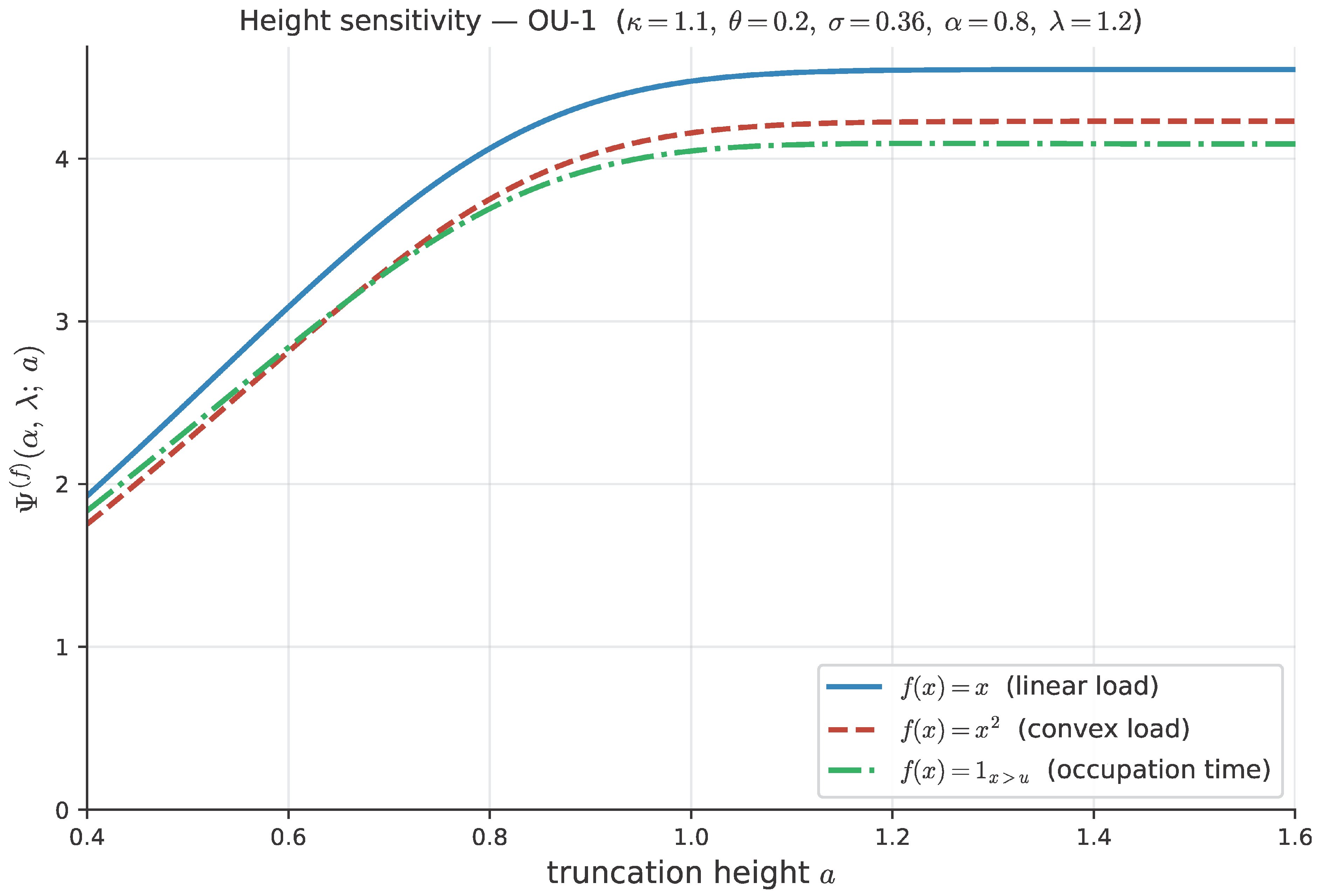
6.2.1. Sensitivity to the Truncation Height $a$

Figure 1 plots $a\mapsto {\Psi }_{\alpha ,\lambda ;a}^f$ for $a\in \left[0.4,1.6\right]$, under the OU-1 baseline

$$\kappa =1.1, \theta =0.2, \sigma =0.36, \alpha =0.8, \lambda =1.2,$$

(152)

with a relative alert level $u=0.6a$. The monotone increase in $a$ is the expected inclusion effect: enlarging the cap admits more subcritical excursions and hence increases the truncated excursion mass. The comparison between marks is also informative:

-

$f\left(x\right)=x$ captures total burden and increases smoothly with $a$;

-

$f\left(x\right)=x^2$ is more sensitive to excursions near the upper part of $\left[0,a\right]$;

-

$f\left(x\right)=1_{\{x>u\}}$ is threshold-oriented and saturates earlier when $u$ scales with $a$.

This is the threshold-calibration sensitivity relevant in both application classes of Section 6.1.

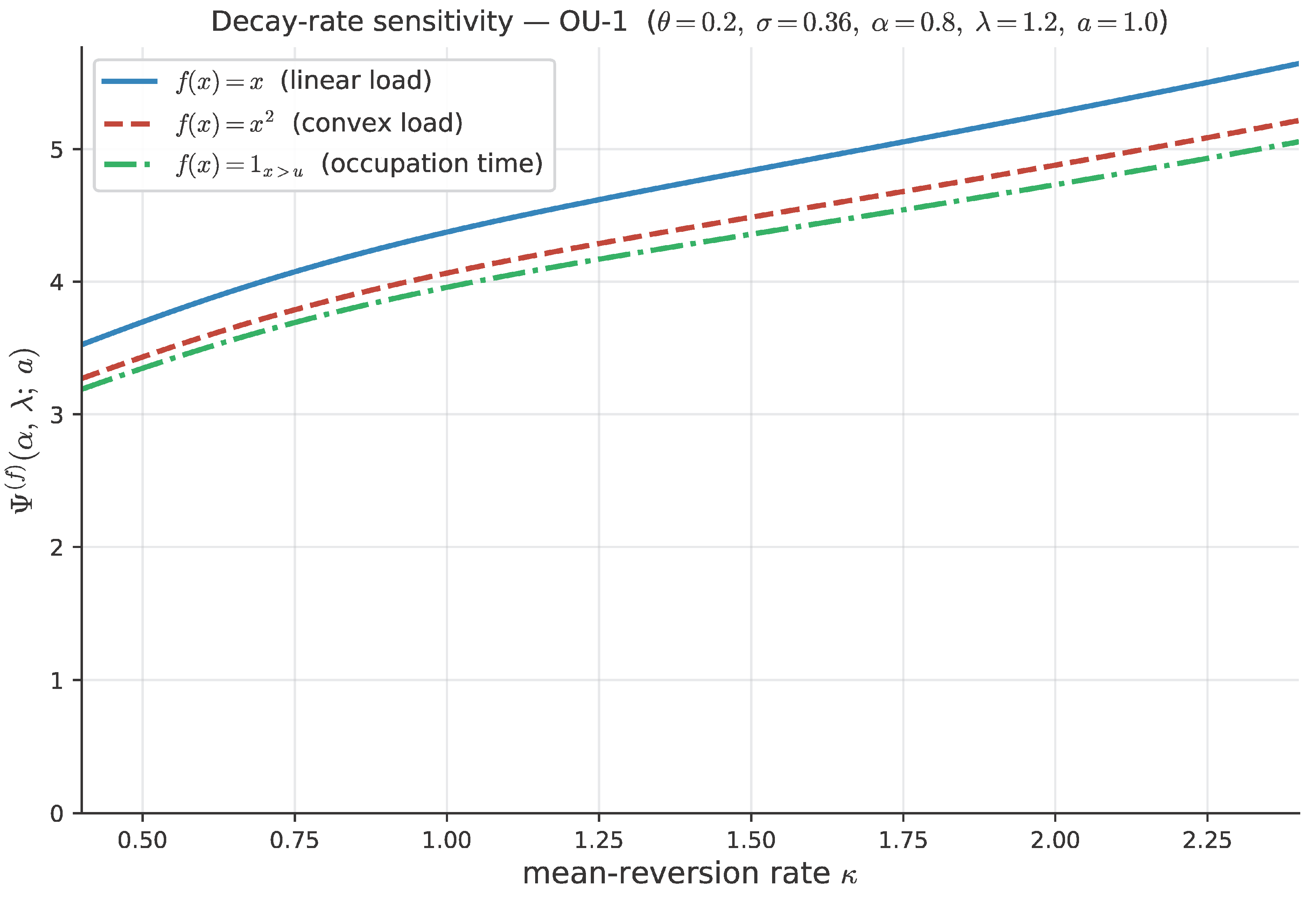
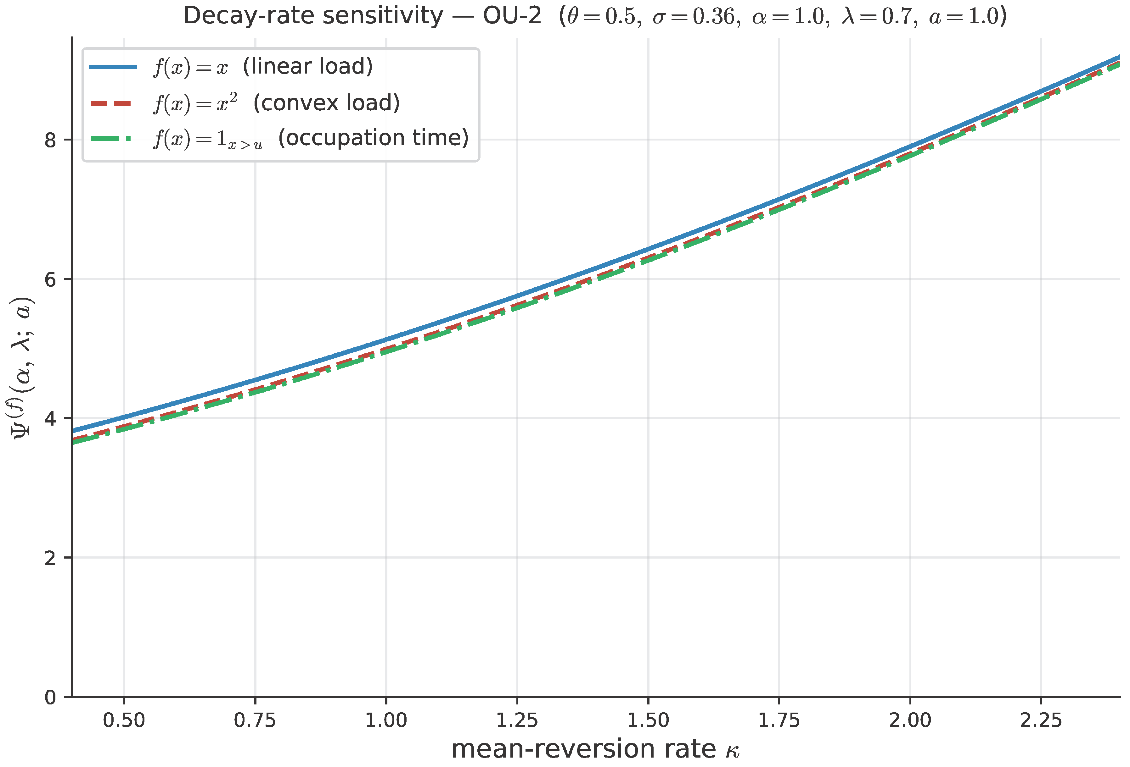
6.2.2. Sensitivity to the Mean-Reversion (Decay) Parameter $\kappa$

Figure 2 fixes $a=1$, $u=0.6$, $\theta =0.2$, $\sigma =0.36$, $\alpha =0.8$, $\lambda =1.2$, and varies $\kappa$ over the displayed range. For this baseline, all three exponents increase with $\kappa$. In the present normalization, stronger mean reversion changes the excursion geometry in a way that increases the effective killing contribution per excursion under the chosen transform parameters.

The three marks remain quantitatively distinct:

-

$f\left(x\right)=x$ is uniformly largest (here $a=1$, so $x\ge x^2$ on $\left[0,1\right]$);

-

$f\left(x\right)=x^2$ is smaller and more amplitude-selective;

-

$f\left(x\right)=1_{\{x>u\}}$ is close in scale to $x^2$ but exhibits a different $\kappa$-profile.

These curves provide a direct comparison across recovery-speed scenarios (market normalization, damping/cooling intensity) under different burden metrics.

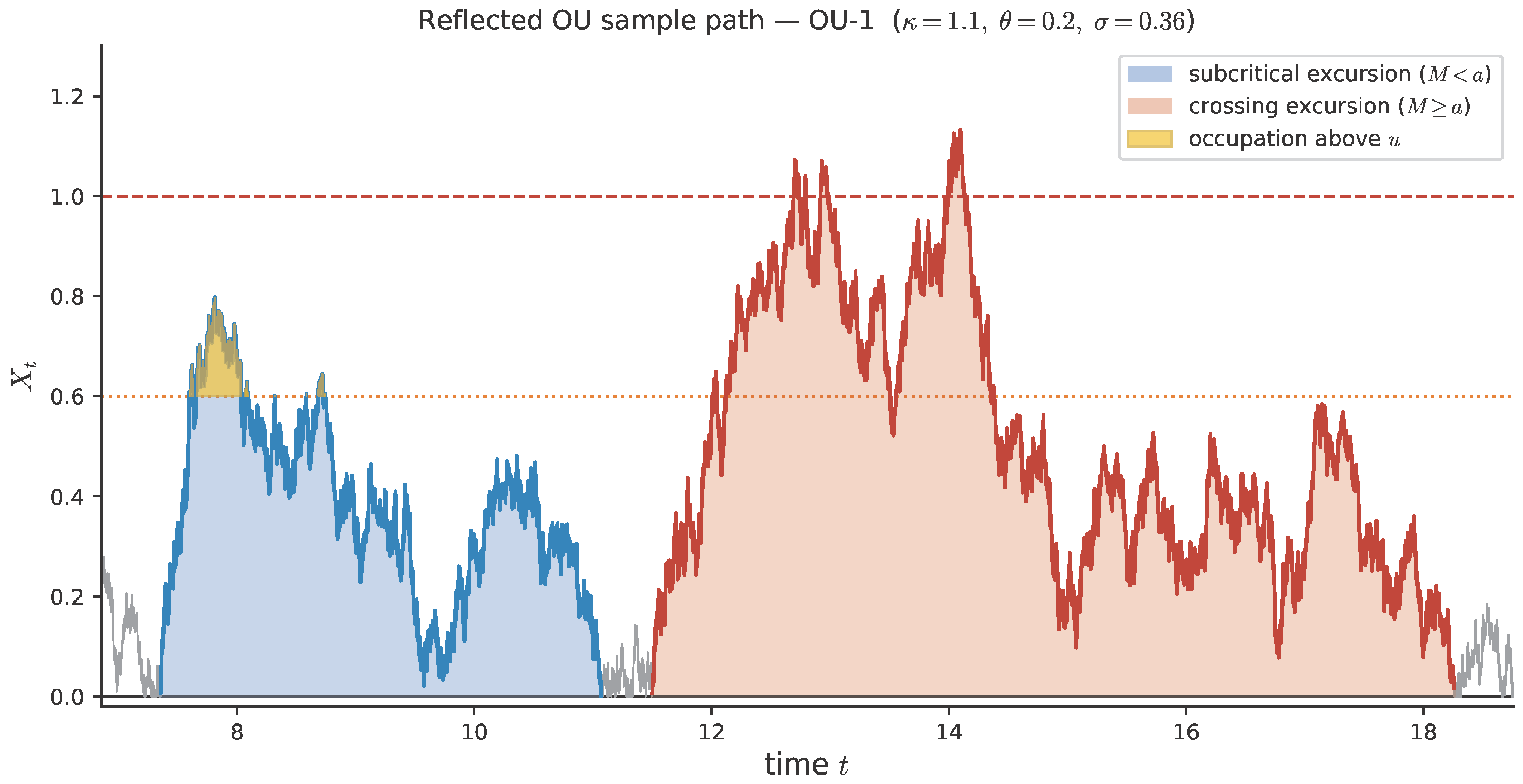
6.2.3. Path-Level Interpretation of Truncation and Occupation Time

Figure 3 shows a simulated reflected OU path segment for the OU-1 baseline, with $a=1$, $u=0.6$, and $\Delta t={10}^{-3}$. The figure highlights one subcritical excursion ($M<a$) and one crossing excursion ($M\ge a$), together with the portion of the retained excursion above $u$, corresponding to the occupation-time mark $f\left(x\right)=1_{\{x>u\}}$. This panel gives an immediate visual interpretation of the truncation rule and the indicator mark.

6.2.4. Robustness Under a Second OU Parameter Set

Figure 4 repeats the $\kappa$-sensitivity analysis for a second OU configuration (OU-2), with $\theta =0.5$, $\sigma =0.36$, $\alpha =1.0$, $\lambda =0.7$, and $a=1$. The same qualitative dependence on $\kappa$ is observed, confirming that the behavior in Figure 2 is not specific to the OU-1 baseline.

6.3. From Transforms to Tail Intensities and Extreme-Burst Probabilities

Section 4 reduces the passage from the transform to the tail intensity $n\left[A_f>y;\hspace{0.17em}M<a\right]$ to a one-dimensional Laplace inversion problem (Lemma 1). In this section, we perform that inversion numerically and then apply the PPP formulas of Section 4.1 to obtain extreme-burst distributions.

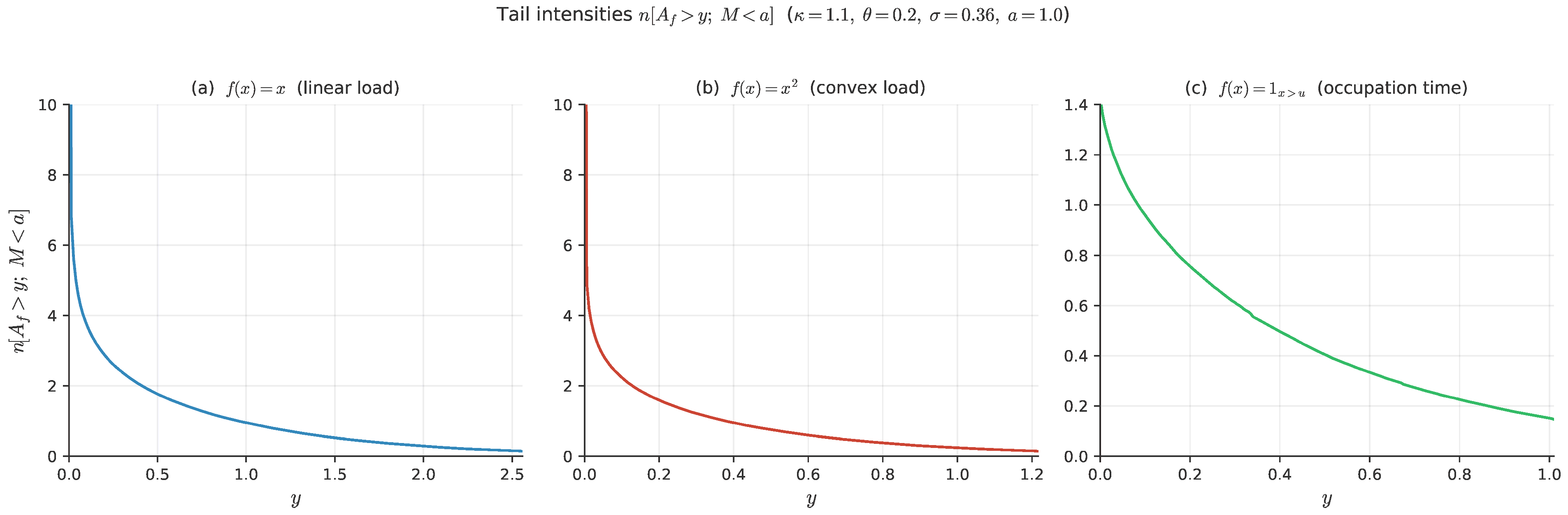
6.3.1. Tail Intensities $n\left[A_f>y; M<a\right]$

Figure 5 reports the reconstructed tails $y\mapsto n\left[A_f>y;\hspace{0.17em}M<a\right]$ for the three marks $f\left(x\right)\in \{x, x^2, {\mathbf{1}}_{\{x>u\}}\}$ under the OU-1 baseline ($\kappa =1.1, \theta =0.2, \sigma =0.36, a=1, u=0.6$). For each mark, the tail intensity $U_f\left(y\right):=n\left[A_f>y;\hspace{0.17em}M<a\right]$ is recovered from Lemma 1 by numerical inversion of the one-dimensional Laplace transform

$${\displaystyle \frac{{\Psi }_{0,\lambda ;a}^f}{\lambda }} (\mathrm{equivalently}, {\Psi }_{0,\lambda ;a}^f=\lambda {\int }_0^{\infty }{e}^{-\lambda y}{U}_f\left(y\right)\hspace{0.17em}dy).$$

(153)

In practice, we evaluate ${\Psi }_{0,\lambda ;a}^f$ with the stabilized boundary–flux pipeline of Section 5.1, apply Abate–Whitt inversion to ${\Psi }_{0,\lambda ;a}^f/\lambda$, and validate the recovered tail by nonnegativity, monotonicity, and forward re-Laplace checks, i.e., numerically re-integrating the recovered tail against exp(−λy) and comparing with the known transform value ${\Psi }_{0,\lambda ;a}^f$ at several test values of λ ∈ {0.5, 1, 2, 5}.

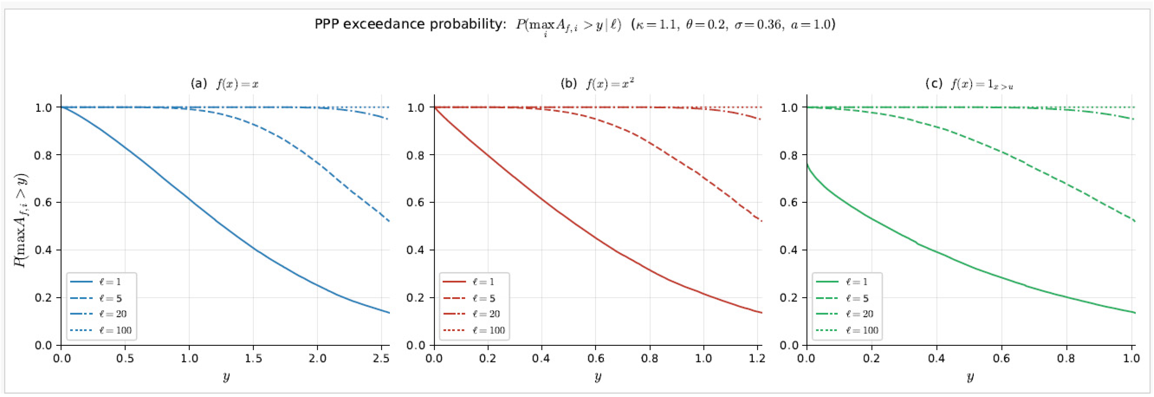
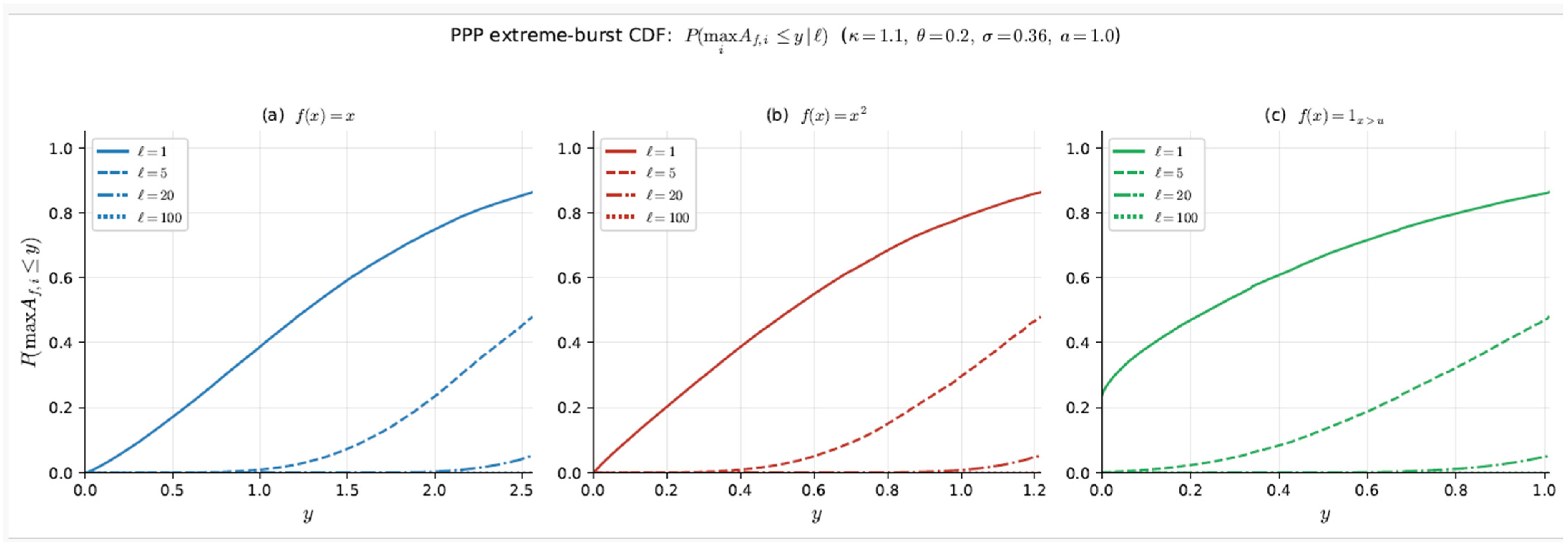
6.3.2. PPP Extreme-Burst Laws

Once $n\left[A_f>y;\hspace{0.17em}M<a\right]$ is available, Proposition 1 gives the law of the largest subcritical burst over local-time horizon $\mathcal{l}$. Figure 6 shows the CDF form

$$\mathbb{P}\left(\underset{i}{\mathrm{m}\mathrm{a}\mathrm{x}}{A}_{f,i}\le y\mid \mathcal{l}\right)=\mathrm{e}\mathrm{x}\mathrm{p}\left(-\mathcal{l}\hspace{0.17em}n\left[A_f>y;\hspace{0.17em}M<a\right]\right),$$

(154)

and Figure 7 shows the equivalent exceedance form

$$\mathbb{P}\left(\underset{i}{\mathrm{m}\mathrm{a}\mathrm{x}}{A}_{f,i}>y\mid \mathcal{l}\right)=1-\mathrm{e}\mathrm{x}\mathrm{p}\left(-\mathcal{l}\hspace{0.17em}n\left[A_f>y;\hspace{0.17em}M<a\right]\right),$$

(155)

for $\mathcal{l}\in \{1,5,20,100\}$. These are direct numerical realizations of the PPP formulas in Section 4, now applied to the OU case study and to all three marks.

From an applied viewpoint, Figure 6 is often the most natural panel: it gives, for any threshold $y$, the probability of at least one large subcritical burst over horizon $\mathcal{l}$, i.e., the near-miss extreme risk emphasized in Section 6.1.

6.3.3. Numerical Inversion Feasibility: Abate–Whitt and Stehfest Algorithms

The practical value of the closed-form Laplace exponents obtained in Section 3, Section 4 and Section 5 depends on whether the corresponding transforms can be inverted numerically with controlled accuracy. In the present setting, the answer is affirmative: the inversion targets are monotone, nonnegative functions (tail intensities and distribution tails), and the transforms are evaluated via the stabilized boundary–flux pipeline of Section 5.1.

We use an adaptive Abate–Whitt algorithm as the default inversion method, already described in Section 5.1. It is stable across the parameter ranges considered, provided the transform is evaluated with the Section 5.1 pipeline (ratio/log evaluation, derivative identities, and conditioning checks). It handles monotone tails naturally: the discretization error is exponentially damped by the Euler weights, and the aliasing error is controlled by the shift c.

A classical Stehfest-type inversion is also feasible and may be used as an auxiliary cross-check on selected parameter sets ([37]). It constructs the inverse from evaluations of the transform on the positive real axis only (no complex arithmetic), via a weighted linear combination of the Gaver functionals G_k(y). However, the weights grow combinatorially and alternate in sign, making the method more sensitive to cancelation, oscillations and finite-precision effects. In the setting of this paper, the boundary–flux transform is built from ratios of ODE solutions over [0, a], and the resulting round-off is amplified by the large alternating Stehfest weights.

Finally, if a mark density is needed, the most robust approach is to invert the tail on a fine grid using the validated Abate–Whitt pipeline and then differentiate numerically (e.g., via finite differences on the inverted values, or by fitting a monotone spline and differentiating analytically). However, density recovery by Laplace inversion is a harder problem than tail recovery. There are three compounding reasons. First, the tail is one degree smoother than the density: it is monotone and continuous for the marks considered here, whereas the density may exhibit interior modes, kinks near the origin, or integrable singularities (as is the case, for instance, for the occupation-time density of a Brownian excursion above a fixed level). Fourier-series inversion methods converge geometrically for smooth targets but degrade to algebraic rates—or develop Gibbs-type oscillations—near non-smooth features of the density. Second, passing from the tail transform to the density transform amounts, in the Laplace domain, to multiplication by s, which amplifies the high-frequency content of the transform. Since the ODE-shooting evaluation of Ψ loses accuracy for large |s| (the potential is dwarfed by Re(s), making the boundary-value problem increasingly stiff), this multiplication precisely amplifies the noisiest part of the transform data. Third, the tail’s nonnegativity and monotonicity provide two automatic post-inversion diagnostics; a density is nonnegative but generally non-monotone, so that small spurious oscillations are harder to distinguish from genuine structure.

6.4. Reproducibility for the OU Case Study

Table 2. Figure-by-figure parameters (Section 6.2 and Section 6.3).

Figure(s)	Purpose	OU/Truncation/Mark Parameters	Transform or Simulation Parameters	Numerical Method/Output
Figure 1	Height sensitivity of ${\Psi }_{\alpha ,\lambda ;a}^f$	OU-1 baseline: $\kappa =1.1,\hspace{0.25em}\theta =0.2,\hspace{0.25em}\sigma =0.36$; marks $f\left(x\right)\in \{x,\hspace{0.25em}{x}^2,\hspace{0.25em}{\mathbf{1}}_{\{x>u\}}\}$; $a\in \left[0.4,1.6\right];$ relative alert level $u=0.6a$	$\alpha =0.8$, $\lambda =1.2$	ODE shooting/boundary–flux evaluation (Section 6.2), with normalization correction $\Psi ={\varphi }_1\left(a\right)/{\varphi }_2\left(a\right)-1/s\left(a\right)$
Figure 2	Decay-rate sensitivity of ${\Psi }_{\alpha ,\lambda ;a}^f$ (OU-1)	$\theta =0.2,\hspace{0.25em}\sigma =0.36,\hspace{0.25em}a=1.0,\hspace{0.25em}u=0.6$; $\kappa \in \left[0.4,2.4\right];$ marks $f\left(x\right)\in \{x,\hspace{0.25em}{x}^2,\hspace{0.25em}{\mathbf{1}}_{\{x>u\}}\}$	$\alpha =0.8$, $\lambda =1.2$	ODE shooting/boundary–flux evaluation (same pipeline as Figure 1)
Figure 3	Path-level illustration of truncation and alert occupancy	OU-1 baseline: $\kappa =1.1,\hspace{0.25em}\theta =0.2,\hspace{0.25em}\sigma =0.36$; cap $a=1.0$; alert $u=0.6$	Path discretization step $\Delta t={10}^{-3}$	Simulated reflected OU path segment; highlights one subcritical excursion ($M<a$) and one crossing excursion ($M\ge a$)
Figure 4	Decay-rate sensitivity (OU-2 robustness panel)	OU-2 parameters shown on plot: $\theta =0.5,\hspace{0.25em}\sigma =0.36,\hspace{0.25em}\alpha =1.0,\hspace{0.25em}\lambda =0.7,\hspace{0.25em}a=1.0$; same three marks $f$	$\kappa$-scan over the plotted range (as displayed on the horizontal axis)	ODE shooting/boundary–flux evaluation (same pipeline as Figure 1 and Figure 2)
Figure 5	Tail intensities $y\mapsto n\left[A_f>y;\hspace{0.17em}M<a\right]$	OU-1 baseline: $\kappa =1.1,\hspace{0.25em}\theta =0.2,\hspace{0.25em}\sigma =0.36,\hspace{0.25em}a=1.0,\hspace{0.25em}u=0.6$; marks $f\left(x\right)\in \{x,\hspace{0.25em}{x}^2,\hspace{0.25em}{\mathbf{1}}_{\{x>u\}}\}$		Excursion-wise mark computation by Riemann summation; empirical tail intensity $\#\{A_f>y\}/L_{\mathrm{t}\mathrm{o}\mathrm{t}}$; forward re-Laplace check vs. ODE values
Figure 6 and Figure 7	PPP extreme-burst laws from Figure 5 tails	Same marks and OU-1 setup as Figure 5	Local-time horizons $\mathcal{l}\in \{1, 5, 20, 100\}$	Figure 6: CDF $\mathrm{e}\mathrm{x}\mathrm{p}\left(-\mathcal{l}\hspace{0.17em}n\left[A_f>y; M<a\right]\right)$; Figure 7: exceedance $1-\mathrm{e}\mathrm{x}\mathrm{p}\left(-\mathcal{l}\hspace{0.17em}n\left[A_f>y; M<a\right]\right)$ (Proposition 1)

and

Table 3. Recommended setting for inversion and simulation.

Component	Recommended Value(s)	Notes
Transform evaluation	NIST/DLMF conventions; ratio-first/logarithmic evaluation; analytic derivative identities (no finite differences for flux); denominator and monotonicity diagnostics	Reuses Section 5.1 conventions
Abate–Whitt inversion target	Invert ${\Psi }_{0,\lambda ;a}^f/\lambda$ to recover $U_f\left(y\right)=n\left[A_f>y;\hspace{0.17em}M<a\right]$ (Lemma 1)	Same pipeline for all three marks; only the ODE/Feynman–Kac transform computation changes
$y$-grid (default)	Log-spaced grid, $N_y=160$ points	Good default value for smooth tails and PPP curves; increase to $N_y=220$ for extra smoothness
Suggested $y$-ranges by mark	$f\left(x\right)=x:\hspace{0.25em}\left[{10}^{-3}, 8\right]$; $f\left(x\right)=x^2:\hspace{0.25em}\left[{10}^{-4}, 4\right]$; $f\left(x\right)={\mathbf{1}}_{\{x>u\}}:\hspace{0.25em}\left[{10}^{-4}, 12\right]$	Practical defaults for the OU-1 case study ($a=1,\hspace{0.25em}u=0.6$); adapt if your final plots use a different visible range
Precision mode	Double precision (default); 50-digit multi-precision fallback/final check if diagnostics fail	Especially useful when cancelation appears in transform evaluation or inversion partial sums
Adaptive stopping	Increase the truncation order until, on the whole $y$-grid, $U_f^{\left(N+\Delta N\right)}\left(y\right)-U_f^{\left(N\right)}\left(y\right)$ $\le {10}^{-6}+{10}^{-4}\hspace{0.17em}\left|U_f^{\left(N+\Delta N\right)}\left(y\right)\right|$ for all (or at least $>95\%$) of grid points
Post-inversion checks	(1) Nonnegativity and monotonicity of $U_f$; (2) On a test set of $\lambda$-values (say 6–10 values over the range used in your plots), require ${\displaystyle \frac{\left|\lambda {\int }_0^{\infty }{e}^{-\lambda y}{U}_f\left(y\right)\hspace{0.17em}dy-{\Psi }_{0,\lambda ;a}^f\right|}{\mathrm{m}\mathrm{a}\mathrm{x}\left(1,\left|{\Psi }_{0,\lambda ;a}^f\right|\right)}}\le {10}^{-3}$
Monte Carlo	Euler–Maruyama for OU; boundary-crossing correction + last-step interpolation; report $\left(T, \Delta t, \mathrm{seed}\right)$ explicitly

below collect the numerical settings and display conventions needed to make the OU illustrations fully reproducible.

7. Discussion and Outlook

This final section discusses directions of research that remain open for future work: broader diffusion settings, richer excursion-mark structures, and asymptotic/inverse questions beyond the scalar-mark framework developed in Section 2, Section 3 and Section 4.

7.1. Extensions of the Boundary–Flux Framework to Broader Diffusion Settings

The boundary–flux principle is not tied to the three explicit model families treated in Section 3. It applies to any regular diffusion admitting a local time at the reference boundary and a well-posed killed Feynman–Kac problem on $\left(0,a\right)$. The main issue is then no longer the probabilistic transfer principle but the tractability of the associated boundary-value problem.

7.1.1. Further Solvable or Semi-Solvable Diffusion Families

A first extension is toward other one-dimensional diffusions whose killed Sturm–Liouville problems remain explicit or spectrally tractable. Natural candidates include constant-elasticity (CEV-type) diffusions and radial/mean-reverting Bessel-type models, for which suitable transforms often reduce the killed ODE to Bessel, Whittaker, or confluent hypergeometric forms [21,22]. Even when closed forms are not available, the boundary–flux representation still reduces the excursion problem to a one-dimensional analytic object, making spectral or asymptotic analysis feasible.

7.1.2. Interior Killing and State-Dependent Discounting

The framework also extends naturally to diffusions with an additional interior killing (or discounting) mechanism. At the Feynman–Kac level, this amounts to adding a nonnegative state-dependent term to the potential, while the excursion-level interpretation remains unchanged: the resulting boundary flux still yields a height-truncated excursion exponent, now incorporating both the mark and the interior killing. This provides a direct route to models where excursions are attenuated or terminated before reaching the height cap.

7.1.3. Elastic or Sticky Reflection at the Boundary

Another important direction is to replace instantaneous reflection at $0$ by elastic or sticky boundary behavior. In such models, the excursion decomposition survives but the local-time normalization and the boundary condition at the reflecting endpoint are modified. Analytically, this typically appears as a Robin-type or transmission-type boundary condition, rather than the normalization used here. The boundary–flux principle should remain the correct organizing device, but the map from the killed boundary-value problem to the excursion exponent must be recalibrated to the chosen local-time convention.

7.1.4. Two-Sided and Interval Diffusions

A further extension is to diffusions on an interval $\left[0, b\right]$ (or more general two-sided settings), where excursions are taken relative to one endpoint while another boundary acts as a truncation or absorption barrier. This would allow nested truncation schemes and intermediate-barrier analyses, and would make the current height-truncation mechanism compatible with finite-domain models in storage, queueing, or constrained physical systems.

7.2. Beyond Scalar Marks: Toward an Excursion-Mark Lévy Theory

Section 4 shows that the combination of excursion PPP structure and boundary–flux Laplace exponents yields, in the scalar-mark case, a unified description of cumulative-load laws and extreme-burst laws. A natural next step is to extend this mechanism into a broader excursion-mark Lévy theory for diffusions.

Section 6 already provides a first indication of this direction by treating several distinct marks (linear load, quadratic load, and occupation time above an alert level) within the same framework. The next theoretical step is to treat such marks jointly rather than one at a time. This suggests introducing multivariate excursion marks and studying the associated joint Laplace exponents, with the aim of deriving:

(i)

joint Lévy measures for marked excursion populations;

(ii)

multivariate extreme-event laws (for example, joint exceedances, coupled maxima, or threshold-crossing sets);

(iii)

dependence structures between marks generated by the same excursion geometry.

At a structural level, this raises a genuinely theoretical question: which Lévy/subordinator laws can arise from diffusion excursions and additive marks via a boundary–flux representation, and what analytic constraints (monotonicity, complete monotonicity, spectral positivity) are inherited from the underlying Sturm–Liouville problem? Even in the scalar case, this can be viewed as a range/characterization problem for the class of Laplace exponents generated by excursion marks.

A further direction is the inverse theory: to what extent does a family of excursion Laplace exponents determine the underlying diffusion (or at least its boundary behavior, scale/speed asymptotics, or mark structure)? Since the present exponents are boundary–flux functionals of killed boundary-value problems, this question is naturally connected to inverse spectral and inverse Sturm–Liouville themes.

7.3. Asymptotic and Structural Questions

The explicit formulas and boundary–flux representations developed here also invite a more systematic asymptotic analysis. Several regimes are particularly natural:

-

large truncation level $a$, where the cap becomes remote and the excursion population approaches an untruncated regime;

-

large-mark tails, relevant for rare but subcritical bursts;

-

weak mean reversion in the OU family, connecting the OU formulas to Brownian-type behavior;

-

boundary-regime limits in BESQ/Bessel-type models, especially near critical parameter values.

More generally, one expects a useful “asymptotic dictionary” linking:

-

boundary behavior of the killed ODE;

-

asymptotics of the boundary–flux Laplace exponent;

-

tail behavior of the induced excursion-mark Lévy measure;

-

and extreme-value regimes in the excursion PPP.

Making this dictionary precise (for instance, via Tauberian arguments tailored to excursion exponents) would provide a conceptual extension of Section 4 and could help identify universality classes of subcritical burst phenomena across different diffusion families and mark choices.

Finally, while the present paper emphasizes explicit solvable families, the boundary–flux formulation is also compatible with spectral methods for general killed diffusions on $\left(0,a\right)$. This suggests a route to extend the current theory beyond closed-form special functions, replacing exact formulas by spectral representations while preserving the excursion interpretation and the PPP/Lévy outputs.

References

- Itô, K. Poisson point processes attached to Markov processes. In Proceedings of the Sixth Berkeley Symposium on Mathematical Statistics and Probability, Vol. III: Probability Theory; University of California Press: Berkeley, CA, USA, 1972; pp. 225–239. [Google Scholar]
- Revuz, D.; Yor, M. Continuous Martingales and Brownian Motion, 3rd ed.; Springer: Berlin/Heidelberg, Germany, 1999. [Google Scholar] [CrossRef]
- Watanabe, S. Itô’s theory of excursion point processes and its applications to Markov processes. Stoch. Process. Appl. 2010, 120, 653–677. [Google Scholar] [CrossRef][Green Version]
- Le Gall, J.-F. Itô’s excursion theory and random trees. Stoch. Process. Appl. 2010, 120, 721–749. [Google Scholar] [CrossRef][Green Version]
- Pitman, J.; Yor, M. A guide to Brownian motion and related stochastic processes. arXiv 2018, arXiv:1802.09679. [Google Scholar] [CrossRef]
- Pitman, J.; Yor, M. Itô’s excursion theory and its applications. Jpn. J. Math. 2007, 2, 83–96. [Google Scholar] [CrossRef]
- Perman, M.; Pitman, J.; Yor, M. Size-biased sampling of Poisson point processes and excursions. Probab. Theory Relat. Fields 1992, 92, 21–39. [Google Scholar] [CrossRef]
- Kallenberg, O. Random Measures, Theory and Applications; Springer: Berlin/Heidelberg, Germany, 2017. [Google Scholar] [CrossRef]
- Lejay, A. The snapping out Brownian motion. Ann. Appl. Probab. 2016, 26, 1727–1742. [Google Scholar] [CrossRef]
- Pilipenko, A.; Sarantsev, A. Boundary approximation for sticky jump-reflected processes on the half-line. Electron. J. Probab. 2024, 29, 1–21. [Google Scholar] [CrossRef]
- Patie, P.; Savov, M.; Zhao, Y. Intertwining, excursion theory and Krein theory of strings for non-self-adjoint Markov semigroups. Ann. Probab. 2019, 47, 3231–3277. [Google Scholar] [CrossRef]
- Profeta, C. The area under a spectrally positive stable excursion and other related processes. Electron. J. Probab. 2021, 26, 1–21. [Google Scholar] [CrossRef]
- Dort, L.; Goldschmidt, C.; Miermont, G. A large deviation principle for the normalized excursion of an alpha-stable Lévy process without negative jumps. ALEA Lat. Am. J. Probab. Math. Stat. 2024, 21, 1625–1653. [Google Scholar] [CrossRef]
- Khanfir, R. Time and place of the maximum for one-dimensional diffusion bridges and meanders. Probab. Surv. 2021, 18, 1–43. [Google Scholar] [CrossRef]
- Louchard, G. Kac’s formula, Lévy’s local time and Brownian excursion. J. Appl. Probab. 1984, 21, 479–499. [Google Scholar] [CrossRef]
- Louchard, G. The Brownian excursion area: A numerical analysis. Comput. Math. Appl. 1984, 10, 413–417. [Google Scholar] [CrossRef]
- Takács, L. A Bernoulli excursion and its various applications. Adv. Appl. Probab. 1991, 23, 557–585. [Google Scholar] [CrossRef]
- Majumdar, S.N.; Comtet, A. Airy distribution function: From the area under a Brownian excursion to the maximal height of fluctuating interfaces. J. Stat. Phys. 2005, 119, 777–826. [Google Scholar] [CrossRef]
- Janson, S. Brownian excursion area, Wright’s constants in graph enumeration, and other Brownian areas. Probab. Surv. 2007, 4, 80–145. [Google Scholar] [CrossRef]
- Janson, S.; Louchard, G. Tail estimates for the Brownian excursion area and other Brownian areas. Electron. J. Probab. 2007, 12, 1600–1632. [Google Scholar] [CrossRef]
- Borodin, A.N.; Salminen, P. Handbook of Brownian Motion-Facts and Formulae, 2nd ed.; Birkhäuser: Basel, Switzerland, 2002. [Google Scholar] [CrossRef]
- Borodin, A.N. Stochastic Processes; Birkhäuser: Basel, Switzerland, 2017. [Google Scholar] [CrossRef]
- Salminen, P.; Vallois, P.; Yor, M. On the excursion theory for linear diffusions. Jpn. J. Math. 2007, 2, 97–127. [Google Scholar] [CrossRef]
- Getoor, R.K.; Sharpe, M.J. Excursions of Brownian motion and Bessel processes. Z. Wahrscheinlichkeitstheor. Verw. Geb. 1979, 47, 83–106. [Google Scholar] [CrossRef]
- Bertoin, J. Lévy Processes; Cambridge University Press: Cambridge, UK, 1996; ISBN 978-0521562430. [Google Scholar]
- Sato, K.-I. Lévy Processes and Infinitely Divisible Distributions; Cambridge University Press: Cambridge, UK, 1999; ISBN 978-0521553025. [Google Scholar]
- Kyprianou, A.E. Fluctuations of Lévy Processes with Applications: Introductory Lectures, 2nd ed.; Springer: Berlin/Heidelberg, Germany, 2014. [Google Scholar] [CrossRef]
- Grebenkov, D.S. Probability distribution of the boundary local time of reflected Brownian motion in Euclidean domains. Phys. Rev. E 2019, 100, 062110. [Google Scholar] [CrossRef] [PubMed]
- Grebenkov, D.S. Paradigm shift in diffusion-mediated surface phenomena. Phys. Rev. Lett. 2020, 125, 078102. [Google Scholar] [CrossRef] [PubMed]
- Durrett, R. Stochastic Calculus: A Practical Introduction; CRC Press: Boca Raton, FL, USA, 1996; ISBN 0-8493-8071-5. [Google Scholar]
- Olver, F.W.J.; Lozier, D.W.; Boisvert, R.F.; Clark, C.W. (Eds.) NIST Handbook of Mathematical Functions; Cambridge University Press: Cambridge, UK, 2010; ISBN 9780521192255. [Google Scholar]
- Alili, L.; Patie, P.; Pedersen, J.L. Representations of the first hitting time density of an Ornstein-Uhlenbeck process. Stoch. Models 2005, 21, 967–980. [Google Scholar] [CrossRef]
- Abate, J.; Whitt, W. Numerical inversion of Laplace transforms of probability distributions. ORSA J. Comput. 1995, 7, 36–43. [Google Scholar] [CrossRef]
- Abate, J.; Valkó, P.P. Multi-precision Laplace transform inversion. Int. J. Numer. Methods Eng. 2004, 60, 979–993. [Google Scholar] [CrossRef]
- Matsumoto, M.; Nishimura, T. Mersenne Twister: A 623-dimensionally equidistributed uniform pseudorandom number generator. ACM Trans. Model. Comput. Simul. 1998, 8, 3–30. [Google Scholar] [CrossRef]
- Gobet, E. Weak approximation of killed diffusion using Euler schemes. Stoch. Process. Appl. 2000, 87, 167–197. [Google Scholar] [CrossRef]
- Stehfest, H. Algorithm 368: Numerical inversion of Laplace transforms. Commun. ACM 1970, 13, 47–49. [Google Scholar] [CrossRef]