The Asymmetric Bimodal Normal Distribution: A Tractable Mixture Model for Skewed and Bimodal Data

Abstract

We study a parsimonious constrained two-component Gaussian mixture with symmetric locations $\pm \lambda$ and unequal weights controlled by $\alpha \in [-1,1]$; we refer to this family as the asymmetric bimodal normal. The constraint eliminates label switching and yields an identifiable parametrization for $\lambda >0$, while noting the boundary degeneracy at $\lambda =0$ where $\alpha$ is not identifiable. We derive closed-form analytical expressions for the density and distribution functions, an equivalent constructive representation (useful for simulation and interpretation), explicit moment formulas, and conditions distinguishing unimodality from bimodality. For inference, we develop maximum likelihood estimation with observed information standard errors and provide numerically stable fits via a block-coordinate quasi-Newton routine using method of moments initial values. A Monte Carlo simulation study across representative parameter settings evaluates bias and root mean squared error, and examines the behavior of Hessian-based standard error estimates, highlighting regimes where the observed information becomes ill-conditioned under weak separation. Empirical analyses, chemical calibration deviations from the National Institute of Standards and Technology and a regression example with asymmetric errors, show competitive or superior fit and interpretability relative to skewed normal alternatives, asymmetric Laplace models, and unconstrained Gaussian mixtures, with consistent advantages under model comparison using the Akaike information criterion and the Bayesian information criterion.

1. Introduction

The modeling of continuous data exhibiting skewness and unimodality or bimodality presents a persistent challenge in applied statistics. Such datasets arise frequently in material reliability and fatigue, neuroscience, finance, and signal processing, where distributions are often characterized by asymmetric tails and potentially overlapping subpopulations. In these contexts, the Gaussian model is insufficient. Although finite Gaussian mixtures offer a versatile baseline, they raise issues of identifiability and interpretability, such as label switching and multimodal likelihood surfaces, that complicate inference and uncertainty quantification [1,2].

Classical results establish conditions for identifiability in finite mixtures and associated pitfalls [3,4]; comprehensive treatments discuss practical implications for estimation and model selection [5,6]. Recent work mitigates some limitations by replacing Gaussian kernels with heavier-tailed or intrinsically skewed components (for example, mixtures based on generalized hyperbolic distributions or normal–inverse Gaussian distributions), thereby improving cluster recovery under asymmetry and contamination [7,8,9,10].

An alternative route relies on skewed but typically unimodal families, most notably the skew-normal and related classes, which offer tractable likelihoods and convenient regression embedding; yet, they do not transparently separate skewness from structural bimodality [11,12,13]. Closer to our construction, two-piece normal extensions provide analytically convenient uni- and bimodal densities with interpretable shape control and have shown practical value in regression and data analysis [14]. When magnitudes are observed in absolute value, the folded normal is a canonical model with a well-developed theory [15,16]; with truncation at zero, a truncated positive normal adds a shape parameter and flexibility for reliability and survival data [17]. Related asymmetric bimodal and two-piece formulations further support disentangling skewness from modality for sharper inference and diagnostics [18,19].

This paper adopts the separation principle and introduces the asymmetric bimodal normal (ABN) family. The model fixes Gaussian locations at $\pm \lambda$ with $\lambda >0$ and controls global asymmetry through mixture weights via $\alpha \in [-1,1]$, thereby side-stepping label switching and preserving interpretability. Although $\alpha$ controls the imbalance of the component weights and $\lambda$ controls the separation of the component means, skewness and modality are not orthogonal: the unimodality-bimodality transition depends jointly on $(\lambda ,\alpha )$ through the critical curve ${\lambda }_c\left(\alpha \right)$ derived in Section 4.2. In particular, increasing $\left|\alpha \right|$ shifts the threshold upward, so strong weight imbalance can suppress bimodality unless $\lambda$ is sufficiently large. Here, $\alpha \in [-1,1]$ guarantees valid mixture weights $(1\pm \alpha )/2\in [0,1]$, while $\lambda >0$ is adopted as an identifiability convention (since $(\lambda ,\alpha )$ and $(-\lambda ,-\alpha )$ yield the same density by swapping component labels). The construction yields a closed-form cumulative distribution function as a convex combination of Gaussian terms, along with a simple stochastic representation clarifying the roles of $(\lambda ,\alpha )$ and providing transparent conditions for unimodality or bimodality. We develop maximum likelihood inference and assess finite-sample behavior (bias, RMSE, coverage) across representative $(\lambda ,\alpha )$ settings, along with real-data illustrations that compare the ABN with skew-normal alternatives and unconstrained Gaussian mixtures. For computation, we rely on L-BFGS-B and block-coordinate updates [20,21,22,23].

Formally, the ABN family is a parsimonious constrained subclass of a two-component Gaussian mixture model with equal variances and symmetric locations. We do not claim that this mixture structure is new in itself; rather, our goal is to provide a unified, tractable, and implementation-oriented treatment for this constrained family, including closed-form distributional expressions, modality characterization, and likelihood-based fitting details. The parametrization $\pm \lambda$ avoids label-switching symmetry and is identifiable for $\lambda >0$; as $\lambda \to 0$, the model collapses to the standard normal, and $\alpha$ becomes non-identifiable, a boundary feature that we explicitly discuss.

To make the connection with existing constrained Gaussian mixtures explicit, consider the symmetric location, equal variance two-normal mixture

$$f_{2N}(z;\lambda ,w)=w\varphi (z-\lambda )+(1-w)\varphi (z+\lambda ),\lambda \ge 0,w\in [0,1].$$

Under the reparametrization $w=(1+\alpha )/2$ (and the identifiability convention $\lambda >0$), this coincides with our ABN family:

$$f_{\mathrm{ABN}}(z;\lambda ,\alpha )={\displaystyle \frac{1+\alpha }{2}}\varphi (z-\lambda )+{\displaystyle \frac{1-\alpha }{2}}\varphi (z+\lambda ),\lambda >0,\alpha \in [-1,1].$$

Equivalently, letting $f_0(z;\lambda )=(\varphi (z-\lambda )+\varphi (z+\lambda ))/2$, we obtain

$$f_{\mathrm{ABN}}(z;\lambda ,\alpha )=f_0(z;\lambda )\left(1+\alpha tanh\left(\lambda z\right)\right),$$

so ABN can be viewed as a bounded, two-parameter reweighting of this constrained mixture; extensions to more general mixtures are left for future work.

This work makes the following contributions, covering both tractable distributional characterization and implementation-oriented inference: (i) we present and study the ABN constrained Gaussian mixture parametrization as an interpretable two-shape-parameter family for asymmetric univariate or bimodal data; (ii) we derive closed-form expressions for the cumulative distribution function and several key analytic characteristics (moments, mgf, and related quantities) and provide an equivalent constructive representation useful for simulation; (iii) we develop and document maximum likelihood estimation with numerically stable implementation details and standard-error computation away from the singular boundary; (iv) we assess finite-sample performance via simulation; and (v) we illustrate practical utility with empirical applications and comparisons to common alternatives.

To avoid any misunderstanding about scope, we emphasize that ABN is a parsimonious constrained two-normal mixture; our focus is tractability and implementation within this subfamily, while more general mixtures are left for future work.

From an applied perspective, the ABN constraint is most attractive when two latent subpopulations can be reasonably approximated by Gaussian components with comparable dispersion and component means that are approximately symmetric around a common center (after location-scale adjustment). In that case, departures from normality can be captured parsimoniously through a single separation parameter (controlling the unimodal–bimodal transition) and a single weight tilt parameter (controlling skewness), yielding an interpretable and identifiable alternative that often stabilizes likelihood optimization relative to a fully unconstrained two-component Gaussian mixture.

Unconstrained two-component Gaussian mixtures allow for distinct locations and scales but introduce label-switching and intertwined shape effects (for example, several parameters working together to determine skewness and the presence of multiple modes). In contrast, ABN fixes symmetric locations and a common variance and uses the two interpretable shape parameters $(\lambda ,\alpha )$. For reference, the univariate skew-normal model [13] has a probability density function (pdf)

$$f_{\mathrm{SN}}(z;\delta )=2\varphi \left(z\right)\mathrm{\Phi }\left(\delta z\right),$$

which accommodates skewness but is essentially unimodal, whereas ABN can transition from unimodality to bimodality through the explicit critical curve ${\lambda }_c\left(\alpha \right)$ (Section 4.2). Moreover, ABN reduces to the equal-weight constrained mixture (the TN baseline) when $\alpha =0$. Section 10 provides empirical benchmarks against common competitors (including skew-normal alternatives, asymmetric Laplace models, and unconstrained Gaussian mixtures).

The remainder of the paper is organized as follows. Section 2 motivates the model and reviews the Gaussian building blocks, the two-piece normal and the folded normal, that underpin the stochastic representation. Section 3 defines the ABN distribution, presents its mixture form and cumulative distribution function, and illustrates the roles of $(\lambda ,\alpha )$. Section 4 collects basic properties, including symmetry relations, limiting behavior, closure properties, and conditions for unimodality versus bimodality. Section 5 derives the Shannon entropy for the ABN family. Section 6 establishes a signed–folded normal representation and a simulation algorithm. Section 7 derives general moment formulae and the moment-generating function, with closed forms for the first four moments and the location–scale extension. Section 8 develops estimation via the method of moments and maximum likelihood, including details on identifiability, optimization, and standard error computation. Section 9 reports a Monte Carlo study of finite-sample performance and numerical stability. Section 10 presents empirical applications on goodness-of-fit assessment and regression with errors following the ABN distribution, benchmarked against competing models. Section 11 concludes with limitations and directions for future work.

2. Motivation and Preliminaries

Our goal is to develop a parsimonious normal-based model with two interpretable shape controls: a modality parameter $\lambda >0$ governing the separation between component centers (unimodality vs. bimodality) and an asymmetry parameter $\alpha \in [-1,1]$ that tilts the mixture weights.

In many applications, departures from normality arise through skewness and/or the presence of two peaks. Classical skew-normal-type families capture skewness but are essentially unimodal, whereas unconstrained two-component Gaussian mixtures can be bimodal but often reduce interpretability and introduce label-switching and intertwined shape effects. The proposed ABN family aims at an intermediate goal: a minimal two-shape-parameter model in which $\alpha$ controls weight imbalance (skewness) and $\lambda$ controls component separation (tendency to bimodality), while preserving tractable closed-form expressions used later for inference and computation.

The preliminaries below are included because the ABN density admits a compact hyperbolic form: the equal-weight symmetric two-normal mixture satisfies $\varphi (x-\lambda )/2+\varphi (x+\lambda )/2=\varphi \left(x\right)exp(-{\lambda }^2/2)cosh\left(\lambda x\right)$.

Allowing unequal weights naturally yields the combination $cosh\left(\lambda x\right)+\alpha sinh\left(\lambda x\right)$ used in Definition 3. The folded normal kernel arises from the transformation $\left|U\right|$ with U normal and underpins the signed folded representation and the simulation algorithm in Section 6; hence, we recall these two Gaussian-based kernels next.

We begin with the symmetric two-piece normal kernel, which is algebraically equivalent to an equal-weight two-normal mixture and will serve as a baseline for introducing the asymmetrical extension.

Definition 1.

A random variable X is said to follow the symmetric two-piece normal distribution, denoted by $X\sim TN\left(\lambda \right)$, if its pdf is given by

$$f_X(x;\lambda )=\varphi \left(x\right)e^{-{\lambda }^2/2}cosh\left(\lambda x\right),x\in \mathbb{R},\lambda \ge 0,$$

(1)

where $\varphi \left(·\right)$ is the standard normal pdf. Using the identity $cosh\left(t\right)=(e^t+e^{-t})/2$, this density can be expressed as an equal-weight mixture of two displaced normal components:

$$f_X(x;\lambda )=\frac{1}{2}\varphi (x-\lambda )+\frac{1}{2}\varphi (x+\lambda ),$$

(2)

which corresponds to an equiprobable mixture of $N(\lambda ,1)$ and $N(-\lambda ,1)$. The parameter $\lambda$ controls the separation between components and, consequently, the transition from unimodality to bimodality (see [14]). In particular, for the equal-weight, equal variance mixture in (2), the density is unimodal if and only if $\lambda \le 1$, and it is bimodal if and only if $\lambda >1$. Equivalently, for the mixture $N({\mu }_1,{\sigma }^2)/2+N({\mu }_2,{\sigma }^2)/2$, the distribution is unimodal if and only if $|{\mu }_1-{\mu }_2|\le 2\sigma$. In (2), we have $|{\mu }_1-{\mu }_2|=2\lambda$ with $\sigma =1$.

Next, we recall the folded normal distribution, whose hyperbolic form mirrors the previous kernel and will be used in the signed folded representation and simulation procedure.

Definition 2.

Let $U\sim N(\mu ,{\sigma }^2)$. The random variable $Y=\left|U\right|$ is said to follow the folded normal distribution, denoted by $Y\sim FN(\mu ,\sigma )$ (see [15]). Its pdf is given by

$$f_Y(y;\mu ,\sigma )={\displaystyle \frac{1}{\sigma }}\sqrt{{\displaystyle \frac{2}{\pi }}}exp\left(-{\displaystyle \frac{y^2+{\mu }^2}{2{\sigma }^2}}\right)cosh\left({\displaystyle \frac{\mu }{{\sigma }^2}}y\right),y>0.$$

By introducing the parameter $\lambda =\mu /\sigma$, we obtain the reparameterized density for $Y\sim FN(\lambda ,\sigma )$:

$$f_Y(y;\lambda ,\sigma )={\displaystyle \frac{2}{\sigma }}\varphi \left({\displaystyle \frac{y}{\sigma }}\right)e^{-{\lambda }^2/2}cosh\left(\lambda {\displaystyle \frac{y}{\sigma }}\right),y>0.$$

(3)

Remark 1.

For $Y\sim FN(\lambda ,1)$,

$$f_Y(y;\lambda )=\varphi (y-\lambda )+\varphi (y+\lambda ),y>0,\lambda \ge 0,$$

(4)

which mirrors the mixture form in (2) restricted to $y>0$.

Definitions 1 and 2 provide the two Gaussian-based kernels that underpin our construction of the ABN family (Definition 3). Definition 1 introduces the symmetric equal-weight mixture $f_X(x;\lambda )=\frac{1}{2}\varphi (x-\lambda )+\frac{1}{2}\varphi (x+\lambda )$, which can be rewritten using $\varphi (x\mp \lambda )=\varphi \left(x\right)exp(-{\lambda }^2/2)exp(\pm \lambda x)$ as $f_X(x;\lambda )=\varphi \left(x\right)exp(-{\lambda }^2/2)cosh\left(\lambda x\right)$. To obtain the asymmetric extension in Definition 3, we retain the same symmetric component locations $\pm \lambda$ and introduce a weight tilt $\alpha \in [-1,1]$:

$$\begin{array}{cc}\hfill f_Z(z;\lambda ,\alpha )& ={\displaystyle \frac{1+\alpha }{2}}\varphi (z-\lambda )+{\displaystyle \frac{1-\alpha }{2}}\varphi (z+\lambda )\hfill \\ \hfill & =\varphi \left(z\right)exp(-{\lambda }^2/2)\left(cosh\left(\lambda z\right)+\alpha sinh\left(\lambda z\right)\right).\hfill \end{array}$$

Finally, Definition 2 is included because the absolute value transformation naturally produces the folded normal kernel; indeed, for $Y=\left|Z\right|$, one has $f_Y\left(y\right)=f_Z\left(y\right)+f_Z(-y)$ for $y>0$, which recovers the mixture form in Remark 1. This connection is exploited later to obtain the signed folded representation and an efficient simulation scheme.

3. The Asymmetric Bimodal Normal Distribution

In this section, we define and study the ABN distribution.

Definition 3.

A random variable Z follows the ABN distribution with parameters $(\lambda ,\alpha )$, denoted $Z\sim ABN(\lambda ,\alpha )$, if its pdf is

$$f_Z(z;\lambda ,\alpha )=\varphi \left(z\right)e^{-{\lambda }^2/2}\left(cosh\left(\lambda z\right)+\alpha sinh\left(\lambda z\right)\right),z\in \mathbb{R},\lambda >0,\left|\alpha \right|\le 1,$$

(5)

where ϕ is the standard normal pdf.

Remark 2.

Using $cosht=(e^t+e^{-t})/2$ and $sinht=(e^t-e^{-t})/2$, (5) is the convex combination

$$f_Z(z;\lambda ,\alpha )={\displaystyle \frac{1+\alpha }{2}}\varphi (z-\lambda )+{\displaystyle \frac{1-\alpha }{2}}\varphi (z+\lambda ),$$

(6)

that is, a combination of $N(\lambda ,1)$ and $N(-\lambda ,1)$ with weights $(1+\alpha )/2$. Accordingly, ABN is a two-parameter constrained Gaussian mixture with symmetric component means; throughout, the study focuses on tractable characterization and inference within this constrained subfamily (rather than on proposing a new mixture structure). Hence, α controls asymmetry (weight imbalance), and $\lambda >0$ controls component separation and modality. At $\alpha =0$, the model coincides with the symmetric equal weight case described in Definition 1. 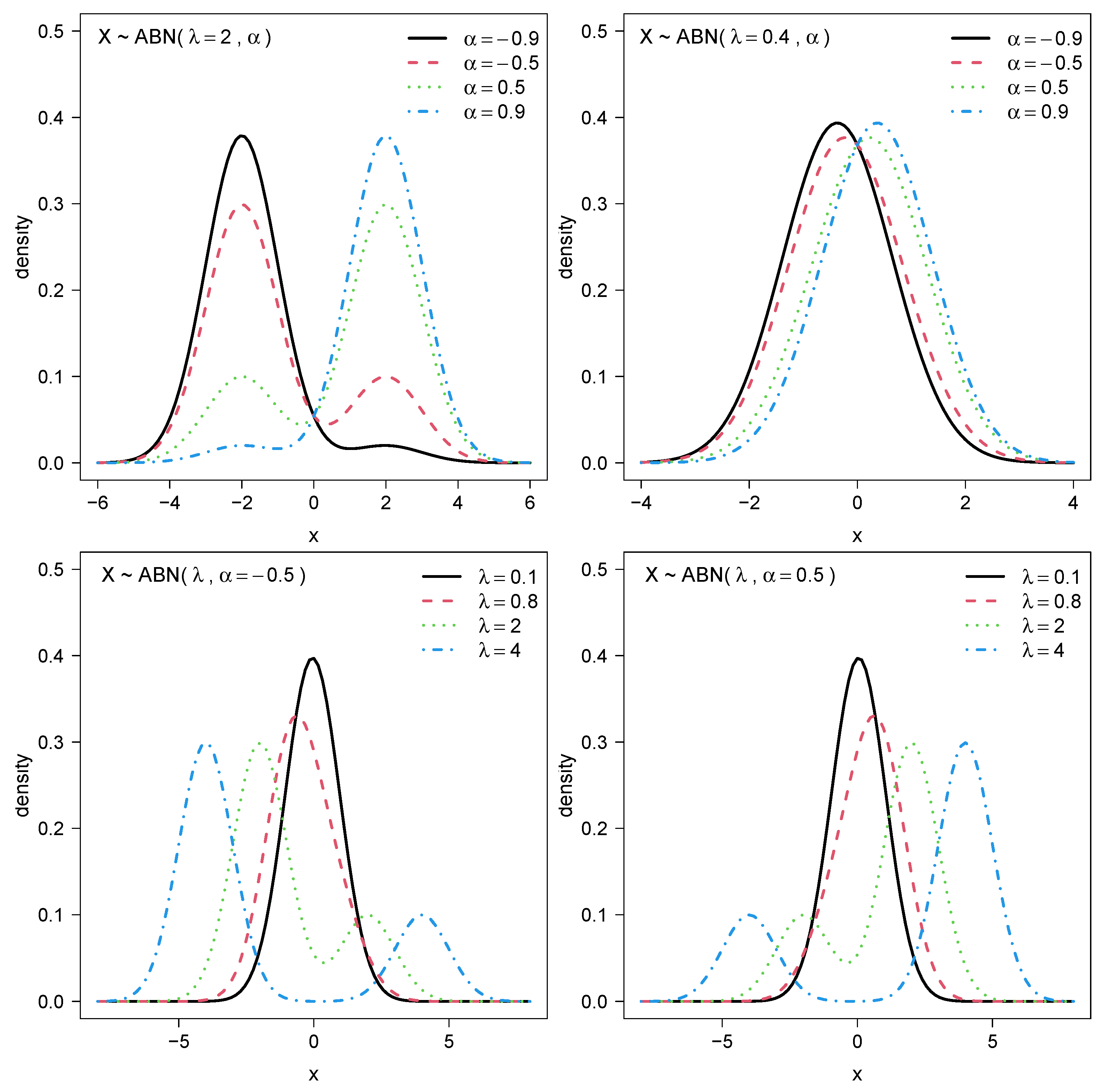At $\lambda =0$, (6) gives $f_Z\left(z\right)=\varphi \left(z\right)$; thus, α is not identifiable on that boundary, and we work with $\lambda >0$ in the full model.

Figure 1 illustrates the roles of the two shape parameters. For fixed $\lambda$ (top panels), varying $\alpha$ tilts the mixture weights and induces left/right asymmetry ($\alpha >0$ shifts probability toward larger values; $\alpha <0$ toward smaller values; $\alpha =0$ is symmetric). For fixed $\alpha$ (bottom panels), increasing $\lambda$ separates the component centers, transitioning from unimodal to bimodal shapes as the separation increases. Proposition 1 provides a closed-form expression for the cumulative distribution function.

Proposition 1.

If $Z\sim ABN(\lambda ,\alpha )$, then the cdf is

$$F_Z(z;\lambda ,\alpha )={\displaystyle \frac{1+\alpha }{2}}\mathrm{\Phi }(z-\lambda )+{\displaystyle \frac{1-\alpha }{2}}\mathrm{\Phi }(z+\lambda ),$$

(7)

where Φ denotes the standard normal cdf.

Remark 3.

The quantile function for the $ABN(\lambda ,\alpha )$ distribution does not admit a closed-form expression. However, since the cdf $F_Z(·;\lambda ,\alpha )$ in (7) is explicit and strictly increasing, the p-th quantile $q_p$ can be straightforwardly found by numerical inversion, that is, as the unique solution of $F_Z(q_p;\lambda ,\alpha )=p$. In practice, robust monotone root-finding methods (for instance, the bisection method or Brent’s algorithm) may be applied. For instance, in R [23], one may implement $F_Z(z;\lambda ,\alpha )$ via pnorm and compute $q_p$ using uniroot applied to $z\mapsto F_Z(z;\lambda ,\alpha )-p$; a self-contained implementation (pABN and qABN) is provided in Appendix B. Random generation is also straightforward. Using the mixture representation in (6), draw $B\sim \mathrm{Bernoulli}\left(\right(1+\alpha )/2)$ and then sample $Z\left|\right\{B=1\}\sim N(\lambda ,1)$ and $Z\left|\right\{B=0\}\sim N(-\lambda ,1)$. For the general location-scale family $X=\xi +\eta Z$, output $X=\xi +\eta Z$. An R routine (rABN) is provided in Appendix B, and Algorithm 1 provides an equivalent sampler based on Proposition 11 and is the one used in the simulation study.

Algorithm 1 Random generation from $X\sim ABN(\xi ,\eta ,\lambda ,\alpha )$.

Require: $\xi \in \mathbb{R}$, $\eta >0$, $\lambda >0$, $\alpha \in [-1,1]$, sample size n   1: for  $i=1,\dots ,n$  do   2:        Generate $U_i\sim \mathcal{N}(\lambda ,1)$ and set $Y_i\leftarrow \left|U_i\right|$   3:        Generate $S_i\sim \mathrm{Bernoulli}\left({\displaystyle \frac{1+\alpha tanh\left(\lambda Y_i\right)}{2}}\right)$   4:        Set $Z_i\leftarrow (2S_i-1)Y_i$                 ▹$Z_i=Y_i$ if $S_i=1$, else $Z_i=-Y_i$   5:        Set $X_i\leftarrow \xi +\eta Z_i$   6: end for   7: return  $X_1,\dots ,X_n$

4. Properties, Closure, and Transformations

We gather fundamental characteristics of the ABN family, focusing on symmetries, limiting behavior, and stability under basic transformations. Throughout, $Z\sim ABN(\lambda ,\alpha )$ denotes the standard version with pdf (6) and cdf (7). The properties collected in this section clarify the interpretation and practical scope of the ABN family. They highlight how $\alpha$ controls weight imbalance (skewness) and how $\lambda$ controls component separation and the uni-/bimodality transition, including informative limiting regimes. They also document key closure behavior under location-scale transformations and additive Gaussian noise, and provide Gaussian-based transformations (absolute value and truncation) that are useful for computation and simulation. Finally, the lack of closure under convolution delineates when richer mixture extensions may be needed.

Proposition 2.

If $Z\sim ABN(\lambda ,\alpha )$ with $\lambda >0$ and $\alpha \in [-1,1]$, then:

(i) 

Symmetric case: $f_Z(z;\lambda ,0)=\varphi \left(z\right)e^{-{\lambda }^2/2}cosh\left(\lambda z\right)$.

(ii) 

Extreme weights: $f_Z(z;\lambda ,1)=\varphi (z-\lambda )$ and $f_Z(z;\lambda ,-1)=\varphi (z+\lambda )$.

(iii) 

Magnitude: $\left|Z\right|\stackrel{d}{=}\left|X\right|\sim FN(\lambda ,1)$, where $X\sim N(\lambda ,1)$ (hence, the law of $\left|Z\right|$ does not depend on α).

(iv) 

Reflection: $-Z\sim ABN(\lambda ,-\alpha )$; equivalently, $f_{-Z}\left(z\right)=\varphi \left(z\right)e^{-{\lambda }^2/2}\left(cosh\left(\lambda z\right)-\alpha sinh\left(\lambda z\right)\right)$.

(v) 

Small-separation limit: ${lim}_{\lambda \to 0^{+}}{f}_Z(z;\lambda ,\alpha )=\varphi \left(z\right)$ for any $\alpha \in [-1,1]$ (the skewness parameter is not identifiable at $\lambda =0$).

(vi) 

Large-separation limit: As $\lambda \to \infty$, the mass escapes to $\pm \infty$: more precisely, $Z/\lambda \Rightarrow S$, where $\mathbb{P}(S=+1)=\frac{1+\alpha }{2}$ and $\mathbb{P}(S=-1)=\frac{1-\alpha }{2}$. In particular, the density does not degenerate at the origin.

Remark 4.

Item (iii) holds for all α because $\left|N\right(\lambda ,1\left)\right|$ and $\left|N\right(-\lambda ,1\left)\right|$ have the same folded normal law. 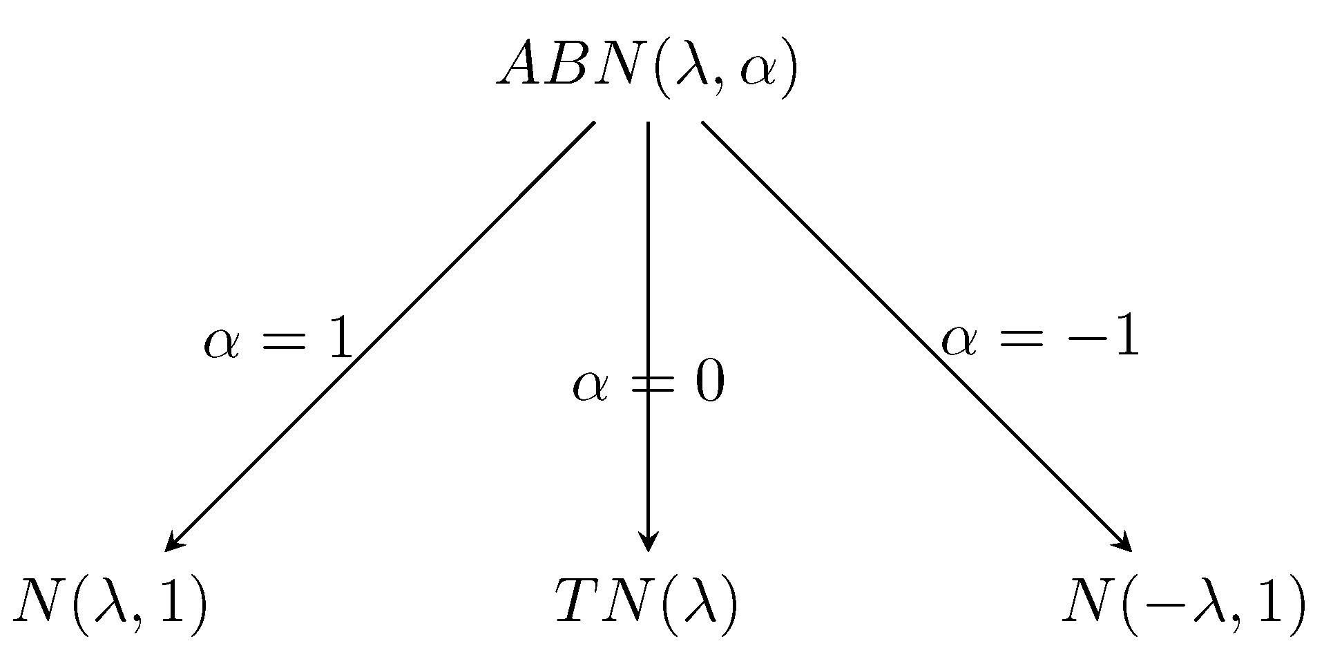The unimodality–bimodality transition is governed by a critical curve ${\lambda }_c\left(\alpha \right)$: in the symmetric case $\alpha =0$, the exact threshold is ${\lambda }_c\left(0\right)=1$, while for imbalanced weights ($\left|\alpha \right|$ close to 1), a larger separation is needed. See Section 4.2 for a sharper characterization and numerical values of ${\lambda }_c\left(\alpha \right)$. We note that alternative numerical thresholds occasionally reported in the literature typically arise from different parameterizations of separation (for instance, by employing a uniform metric to measure the distance between component means); Proposition 8 (i) below provides the self-contained threshold under our $(\pm \lambda ,{\sigma }^2=1)$ convention.

Figure 2 illustrates how the ABN distribution simplifies to other well-known distributions based on specific values of the skewness parameter $\alpha$. When $\alpha =0$, the ABN distribution reduces to the symmetric TN distribution. For extreme cases, when $\alpha =1$, the ABN becomes $N(\lambda ,1)$, and when $\alpha =-1$, it becomes $N(-\lambda ,1)$, highlighting the role of $\alpha$ in selecting the underlying normal component in (6).

4.1. Closure and Transformations

We record the stability properties of the ABN family under basic operations. Closure properties are summarized in Propositions 3–7.

Definition 4.

A random variable X is said to follow an ABN distribution with parameters $\theta =(\xi ,\eta ,\lambda ,\alpha )$, denoted $X\sim ABN\left(\theta \right)$, if its pdf is

$$f_X(x;\theta )={\displaystyle \frac{1}{\eta }}\varphi \left({\displaystyle \frac{x-\xi }{\eta }}\right)exp\left(-{\displaystyle \frac{{\lambda }^2}{2}}\right)\left(cosh\left(\lambda {\displaystyle \frac{x-\xi }{\eta }}\right)+\alpha sinh\left(\lambda {\displaystyle \frac{x-\xi }{\eta }}\right)\right),x\in \mathbb{R},$$

where $\xi \in \mathbb{R}$, $\eta >0$, $\lambda >0$, and $\left|\alpha \right|\le 1$. Equivalently,

$$f_X(x;\theta )={\displaystyle \frac{1+\alpha }{2\eta }}\varphi \left({\displaystyle \frac{x-\xi }{\eta }}-\lambda \right)+{\displaystyle \frac{1-\alpha }{2\eta }}\varphi \left({\displaystyle \frac{x-\xi }{\eta }}+\lambda \right).$$

Proposition 3.

Let $X=\xi +\eta Z$ with $\eta >0$ and $Z\sim ABN(\lambda ,\alpha )$. Then $X\sim ABN(\xi ,\eta ,\lambda ,\alpha )$ (Definition 4). In particular, standardization is exact: $(X-\xi )/\eta \sim ABN(\lambda ,\alpha )$.

Proof. 

Immediately from (6) by changing variables.    □

Proposition 4.

(i) $-Z\sim ABN(\lambda ,-\alpha )$;    (ii) $\left|Z\right|\stackrel{d}{=}\left|N(\lambda ,1)\right|\sim FN(\lambda ,1)$ (independent of α).

Proof. 

(i) Replace z with $-z$ in (6). (ii) Both mixture components yield the same folded normal on $(0,\infty )$; see Remark 4.    □

Proposition 5.

Let $\epsilon \sim N(0,{\tau }^2)$ be independent of Z, and set $X=Z+\epsilon$. Then

$$X\stackrel{d}{=}{\displaystyle \frac{1+\alpha }{2}}N(\lambda ,1+{\tau }^2)+{\displaystyle \frac{1-\alpha }{2}}N(-\lambda ,1+{\tau }^2).$$

Consequently, after variance standardization,

$$X^{✶}={\displaystyle \frac{X}{\sqrt{1+{\tau }^2}}}\sim ABN\left({\displaystyle \frac{\lambda }{\sqrt{1+{\tau }^2}}},\alpha \right).$$

Proof. 

Convolution preserves each Gaussian component and the weights; rescale by $\sqrt{1+{\tau }^2}$ to match the unit component variance ABN template.    □

Proposition 6.

Let $Z_0=Z\mid (Z>0)$. Then $Z_0$ is a two-point mixture of truncated normals:

$$f_{Z_0}\left(z\right)={\displaystyle \frac{1+\alpha }{2p_0}}\varphi (z-\lambda )+{\displaystyle \frac{1-\alpha }{2p_0}}\varphi (z+\lambda ),z>0,$$

where $p_0={\displaystyle \frac{1+\alpha }{2}}\mathrm{\Phi }\left(\lambda \right)+{\displaystyle \frac{1-\alpha }{2}}\mathrm{\Phi }(-\lambda )$. An analogous expression holds for $Z\mid (Z<0)$.

Proof. 

Use (6) and $P\left(N\right(\mu ,1)>0)=\mathrm{\Phi }\left(\mu \right)$ for each component; renormalize by $p_0$.    □

Proposition 7.

Let $Z_1\sim ABN({\lambda }_1,{\alpha }_1)$ and $Z_2\sim ABN({\lambda }_2,{\alpha }_2)$ be independent. Then $Z_1+Z_2$ is, in general, a four-component Gaussian mixture with a common variance 2; hence, it is not $ABN$. Closure holds only when (i) ${\lambda }_1=0$ or ${\lambda }_2=0$ (one factor is normal), or (ii) $|{\alpha }_1|=|{\alpha }_2|=1$ (both factors are normal).

Proof. 

By independence and (6), the sum has support on $\{\pm {\lambda }_1\pm {\lambda }_2\}$ with four weights unless a component collapses to a single normal (cases (i):(ii)). A two-location ABN representation is generally impossible.    □

Remark 5.

Proposition 5 shows that additive Gaussian noise shrinks the separation parameter from λ to $\lambda /\sqrt{1+{\tau }^2}$ without altering α after standardization. Hence, modest measurement noise moves the model toward unimodality (see Section 4.2), a useful diagnostic when comparing raw vs. denoised data.

4.2. Characterization and Bimodality

We collect the structural properties of the ABN family and provide a unified characterization of the transition between unimodality and bimodality.

Proposition 8.

Let $Z\sim ABN(\lambda ,\alpha )$ with pdf (6).

(i) 

Symmetric case: If $\alpha =0$, the density is unimodal if and only if $\lambda \le 1$ and bimodal if and only if $\lambda >1$.

(ii) 

General case: If $\alpha \in (-1,1)$, there exists a unique threshold ${\lambda }_c\left(\alpha \right)\ge 1$, strictly increasing in $\left|\alpha \right|$, such that the density is unimodal if and only if $\lambda \le {\lambda }_c\left(\alpha \right)$ and bimodal if and only if $\lambda >{\lambda }_c\left(\alpha \right)$. In particular, ${\lambda }_c\left(0\right)=1$ and ${lim}_{\left|\alpha \right|\to 1}{\lambda }_c\left(\alpha \right)=\infty$.

(iii) 

Extreme weights: If $\alpha =\pm 1$, then $Z\sim N(\pm \lambda ,1)$, and the density is always unimodal.

(iv) 

Critical curve (implicit form): For $\alpha \in (-1,1)$, the transition occurs at the unique pair $(\lambda ,z_{✶})$, solving

$$\begin{array}{cc}\hfill log\left({\displaystyle \frac{1+\alpha }{1-\alpha }}\right)+log\left({\displaystyle \frac{z_{✶}-\lambda }{z_{✶}+\lambda }}\right)+2\lambda z_{✶}& =0,\hfill \end{array}$$

(8)

$$\begin{array}{cc}\hfill z_{✶}^2& ={\lambda }^2-1,z_{✶}sign\left(\alpha \right)\ge 0,\hfill \end{array}$$

(9)

and ${\lambda }_c\left(\alpha \right)$ is λ, solving (8) and (9).

Proof. 

Write the standard ABN density in mixture form $f_Z\left(z\right)=w_1\varphi (z-\lambda )+w_0\varphi (z+\lambda ),w_1=(1+\alpha )/2,w_0=(1-\alpha )/2$ with $\lambda >0$ and $\alpha \in [-1,1]$. Differentiating, $f_Z^{\prime }\left(z\right)=-w_1(z-\lambda )\varphi (z-\lambda )-w_0(z+\lambda )\varphi (z+\lambda )$. Since this is a two-component equal variance Gaussian mixture, $f_Z$ can have at most two modes.

(i)

In the symmetric case $w_1=w_0=1/2$; hence, $f_Z$ is even and $f_Z^{\prime }\left(0\right)=0$. Moreover,

$$f_Z^{″}\left(0\right)=({\lambda }^2-1)\varphi \left(\lambda \right).$$

Thus, if $\lambda <1$, then $f_Z^{″}\left(0\right)<0$ and 0 is a strict local maximum; by symmetry and the two-mode bound, $f_Z$ is unimodal. If $\lambda >1$, then $f_Z^{″}\left(0\right)>0$ and 0 is a local minimum; since $f_Z\left(z\right)\to 0$ as $\left|z\right|\to \infty$, two symmetric off-zero maxima must occur, hence bimodality. The boundary $\lambda =1$ gives the transition.

(ii)

For $z\in (-\lambda ,\lambda )$, the equation $f_Z^{\prime }\left(z\right)=0$ is equivalent to

$${\displaystyle \frac{w_1}{w_0}}{\displaystyle \frac{\lambda -z}{\lambda +z}}exp\left(2\lambda z\right)=1,$$

using $\varphi (z-\lambda )/\varphi (z+\lambda )=exp\left(2\lambda z\right)$. Define

$$H_{\lambda ,\alpha }\left(z\right):=log\left({\displaystyle \frac{1+\alpha }{1-\alpha }}\right)+log\left({\displaystyle \frac{\lambda -z}{\lambda +z}}\right)+2\lambda z,$$

so that stationary points correspond to zeros of $H_{\lambda ,\alpha }$ in $(-\lambda ,\lambda )$. A direct derivative calculation gives

$$H_{\lambda ,\alpha }^{\prime }\left(z\right)=-{\displaystyle \frac{1}{\lambda -z}}-{\displaystyle \frac{1}{\lambda +z}}+2\lambda =2\lambda \left(1-{\displaystyle \frac{1}{{\lambda }^2-z^2}}\right).$$

If $0<\lambda \le 1$, then ${\lambda }^2-z^2\le {\lambda }^2\le 1$, hence $H_{\lambda ,\alpha }^{\prime }\left(z\right)<0$ for all $z\in (-\lambda ,\lambda )$, and $H_{\lambda ,\alpha }$ has a unique zero. Therefore, $f_Z$ has a unique stationary point and is unimodal.

If $\lambda >1$, then $H_{\lambda ,\alpha }^{\prime }\left(z\right)=0$ occurs at $z=\pm \sqrt{{\lambda }^2-1}$, so $H_{\lambda ,\alpha }$ has one local minimum and one local maximum and therefore has either one zero (unimodal) or three zeros (bimodal). The boundary between these regimes occurs when two zeros merge into a double root; this yields a unique threshold ${\lambda }_c\left(\alpha \right)\ge 1$. The map $\left|\alpha \right|\mapsto {\lambda }_c\left(\alpha \right)$ is strictly increasing because $H_{\lambda ,\alpha }$ depends on $\alpha$ only through the additive term $log\left(\right(1+\alpha )/(1-\alpha \left)\right)$ (increasing in $\left|\alpha \right|$), which shifts the curve and forces the unique double root solution to occur at larger $\lambda$. In particular, ${\lambda }_c\left(0\right)=1$ (from (i)), and ${\lambda }_c\left(\alpha \right)\to \infty$ as $\left|\alpha \right|\to 1$ since $log\left(\right(1+\left|\alpha \right|)/(1-\left|\alpha \right|\left)\right)\to \infty$.

(iii)

One of the mixture weights is zero, hence $Z\sim N(\pm \lambda ,1)$, and the density is unimodal.

(iv)

At the transition in (ii), two stationary points coalesce at $(\lambda ,z^{✶})$, so $f_Z^{\prime }\left(z^{✶}\right)=f_Z^{″}\left(z^{✶}\right)=0$. Solving $f_Z^{\prime }\left(z^{✶}\right)=0$ yields (8), and eliminating the weights via $f_Z^{″}\left(z^{✶}\right)=0$ gives $(z^{✶}+\lambda )(z^{✶}-\lambda )=-1$, hence $z^{✶2}={\lambda }^2-1$, with the branch selection stated in (9). Therefore, ${\lambda }_c\left(\alpha \right)$ is the unique $\lambda$, solving (8) and (9).    □

Remark 6.

Equations (8) and (9) reduce the computation of the critical curve ${\lambda }_c\left(\alpha \right)$ to solving a one-dimensional root-finding problem in $\lambda >1$. In particular, ${\lambda }_c\left(0\right)=1$. For $\alpha \in (-1,1)\setminus \left\{0\right\}$, define

$$G_{\alpha }\left(\lambda \right)=log\left({\displaystyle \frac{1+\alpha }{1-\alpha }}\right)+log\left({\displaystyle \frac{s\left(\lambda \right)-\lambda }{s\left(\lambda \right)+\lambda }}\right)+2\lambda s\left(\lambda \right),s\left(\lambda \right)=sign\left(\alpha \right)\sqrt{{\lambda }^2-1},$$

so that ${\lambda }_c\left(\alpha \right)$ is the unique solution of $G_{\alpha }\left(\lambda \right)=0$ with $\lambda >1$.

In practice, ${\lambda }_c\left(\alpha \right)$ can be computed with a safeguarded Newton method: choose ${\lambda }_L=1+\epsilon$ (for instance, $\epsilon ={10}^{-8}$) and increase ${\lambda }_U$ (for instance, by doubling) until $G_{\alpha }\left({\lambda }_U\right)>0$ (while $G_{\alpha }\left({\lambda }_L\right)<0$ for small ε). Then iterate $\lambda \to \lambda -G_{\alpha }\left(\lambda \right)/G_{\alpha }^{\prime }\left(\lambda \right)$, using the update only if it stays within $({\lambda }_L,{\lambda }_U)$; otherwise, fall back to bisection $\lambda \to ({\lambda }_L+{\lambda }_U)/2$. Update the bracket according to the sign of $G_{\alpha }\left(\lambda \right)$ and stop when $|G_{\alpha }\left(\lambda \right)|$ (or the bracket width) is below a prescribed tolerance. A closed-form derivative is available via

$$s^{\prime }\left(\lambda \right)=sign\left(\alpha \right){\displaystyle \frac{\lambda }{\sqrt{{\lambda }^2-1}}},G_{\alpha }^{\prime }\left(\lambda \right)={\displaystyle \frac{s^{\prime }\left(\lambda \right)-1}{s\left(\lambda \right)-\lambda }}-{\displaystyle \frac{s^{\prime }\left(\lambda \right)+1}{s\left(\lambda \right)+\lambda }}+2s\left(\lambda \right)+2\lambda s^{\prime }\left(\lambda \right).$$

5. Shannon Entropy

An entropy identity is given in Proposition 9, with the location-scale extension in Corollary 1 and a lower bound in Proposition 10. We quantify uncertainty via the Shannon differential entropy. Let $Z\sim ABN(\lambda ,\alpha )$ be the standard version with pdf (6).

Lemma 1.

Let $Z\sim \mathrm{ABN}(\lambda ,\alpha )$ with $\lambda >0$ and $\left|\alpha \right|\le 1$. Define

$$g(u;\alpha )=cosh\left(u\right)+\alpha sinh\left(u\right)={\displaystyle \frac{1+\alpha }{2}}{e}^u+{\displaystyle \frac{1-\alpha }{2}}{e}^{-u},u\in \mathbb{R}.$$

Then $g(u;\alpha )>0$ for all u, so the logarithm inside the expectation term in (10) is well-defined.

If $\left|\alpha \right|<1$ for all $u\in \mathbb{R}$,

$${\displaystyle \frac{1-\left|\alpha \right|}{2}}{e}^{-\left|u\right|}\le g(u;\alpha )\le e^{\left|u\right|},$$

and hence

$$\left|log\left(g\right(u;\alpha \left)\right)\right|\le \left|u\right|+\left|log\left({\displaystyle \frac{1-\left|\alpha \right|}{2}}\right)\right|.$$

Taking $u=\lambda Z$ and using $\mathbb{E}\left(\right|Z\left|\right)<\infty$ (since Z is a two-normal mixture), we get

$$\mathbb{E}\left|log\left(cosh\left(\lambda Z\right)+\alpha sinh\left(\lambda Z\right)\right)\right|<\infty .$$

For $\alpha =\pm 1$, $g(u;\pm 1)=e^{\pm u}$, so $log\left(g\right(\lambda Z\left)\right)=\pm \lambda Z$ and the expectation is also finite.

Proposition 9.

The Shannon entropy of Z is

$$h\left(Z\right)=-\mathbb{E}(log\left(f_Z\left(Z\right)\right))={\displaystyle \frac{1}{2}}log\left(2\pi \right)+{\displaystyle \frac{1}{2}}+{\lambda }^2-\mathbb{E}\left(log\left(cosh\left(\lambda Z\right)+\alpha sinh\left(\lambda Z\right)\right)\right).$$

(10)

In particular, for $\alpha =\pm 1$, one has $h\left(Z\right)={\displaystyle \frac{1}{2}}log\left(2\pi e\right)$ (unit-variance normal), and for $\alpha =0$,

$$h\left(Z\right)={\displaystyle \frac{1}{2}}log\left(2\pi \right)+{\displaystyle \frac{1}{2}}+{\lambda }^2-\mathbb{E}\left(log\left(cosh\left(\lambda Y\right)\right)\right),$$

(11)

where $Y\sim FN(\lambda ,1)$.

Proof. 

From the PDF definition in (5), we have

$$log\left(f_Z\left(Z\right)\right)=-{\displaystyle \frac{1}{2}}log\left(2\pi \right)-{\displaystyle \frac{1}{2}}{Z}^2-{\displaystyle \frac{1}{2}}{\lambda }^2+log\left(cosh\left(\lambda Z\right)+\alpha sinh\left(\lambda Z\right)\right).$$

The entropy is $h\left(Z\right)=-\mathbb{E}(log\left(f_Z\left(Z\right)\right))$. Using the raw second moment $\mathbb{E}\left(Z^2\right)=1+{\lambda }^2$ (Corollary 2), the linear terms become ${\displaystyle \frac{1}{2}}log\left(2\pi \right)+{\displaystyle \frac{1}{2}}(1+{\lambda }^2)+{\displaystyle \frac{1}{2}}{\lambda }^2$, which simplifies to the expression in (10).

For the extreme cases $\alpha =\pm 1$, we use the identity $cosh\left(u\right)\pm sinh\left(u\right)=e^{\pm u}$. The expectation term becomes $\mathbb{E}(log\left(e^{\pm \lambda Z}\right))=\mathbb{E}(\pm \lambda Z)=\pm \lambda \mathbb{E}\left(Z\right)$. Since $\mathbb{E}\left(Z\right)=\alpha \lambda$ and $\alpha =\pm 1$, this equals ${\lambda }^2$. Substituting this back into (10) yields $h\left(Z\right)={\displaystyle \frac{1}{2}}log\left(2\pi \right)+{\displaystyle \frac{1}{2}}+{\lambda }^2-{\lambda }^2={\displaystyle \frac{1}{2}}log\left(2\pi e\right)$.

For the symmetric case $\alpha =0$, the term reduces to $\mathbb{E}(log(cosh\left(\lambda Z\right)\left)\right)$. Since $cosh\left(·\right)$ is an even function, this expectation depends only on the magnitude $\left|Z\right|$. Recalling that $\left|Z\right|\stackrel{d}{=}Y\sim FN(\lambda ,1)$, we obtain (11).    □

Corollary 1.

If $X=\xi +\eta Z\sim ABN(\xi ,\eta ,\lambda ,\alpha )$ with $\eta >0$, then

$$h\left(X\right)=h\left(Z\right)+log\left(\eta \right).$$

(12)

Remark 7.

A numerically integrable function uses the log–sum–exp form

$$log\left(cosh\left(u\right)+\alpha sinh\left(u\right)\right)=LSE\left(log(1+\alpha )+u,log(1-\alpha )-u\right)-log\left(2\right),u=\lambda z.$$

Expectations in (10) can be computed as a two-term Gaussian mixture integral from (6), or via Gauss–Hermite quadrature after the change of variable $z\mapsto z\pm \lambda$.

The next proposition provides a simple closed-form lower bound for the entropy $h\left(Z\right)$ in terms of $(\lambda ,\alpha )$, which is useful for a quick numerical assessment without computing the expectation in (10).

Proposition 10.

Let $Z\sim ABN(\lambda ,\alpha )$ and set $c(\lambda ,\alpha )=cosh\left({\lambda }^2\right)+{\alpha }^{2}sinh\left({\lambda }^2\right)$. Then

$$h\left(Z\right)\ge \frac{1}{2}log\left(2\pi e\right)+\frac{{\lambda }^2}{2}-log\left(c(\lambda ,\alpha )\right).$$

(13)

Proof. 

Let $g\left(z\right)=cosh\left(\lambda z\right)+\alpha sinh\left(\lambda z\right)$. Since $g\left(z\right)=(1+\alpha )e^{\lambda z}/2+(1-\alpha )e^{-\lambda z}/2>0$ for $\left|\alpha \right|\le 1$, $log\left(g\right(Z\left)\right)$ is well-defined and, by the concavity of log, Jensen’s inequality gives

$$\mathbb{E}(log\left(g\left(Z\right)\right))\le log\left(\mathbb{E}\left(g\right(Z\left)\right)\right).$$

Moreover,

$$\mathbb{E}\left(g\left(Z\right)\right)={\displaystyle \frac{1+\alpha }{2}}{M}_Z\left(\lambda \right)+{\displaystyle \frac{1-\alpha }{2}}{M}_Z(-\lambda ),$$

and using the mgf of Z (see Proposition 14, $M_Z\left(t\right)=e^{t^2/2}(cosh\left(\lambda t\right)+\alpha sinh\left(\lambda t\right))$), we obtain $M_Z(\pm \lambda )=e^{{\lambda }^2/2}(cosh\left({\lambda }^2\right)\pm \alpha sinh\left({\lambda }^2\right))$; hence,

$$\mathbb{E}\left(g\left(Z\right)\right)=e^{{\lambda }^2/2}\left(cosh\left({\lambda }^2\right)+{\alpha }^{2}sinh\left({\lambda }^2\right)\right)=e^{{\lambda }^2/2}c(\lambda ,\alpha ).$$

Substituting into the entropy identity (10), $h\left(Z\right)=\frac{1}{2}log\left(2\pi e\right)+{\lambda }^2-\mathbb{E}(log\left(g\left(Z\right)\right))$, yields

$$h\left(Z\right)\ge \frac{1}{2}log\left(2\pi e\right)+{\lambda }^2-\left(\frac{{\lambda }^2}{2}+log\left(c(\lambda ,\alpha )\right)\right),$$

which is (13).    □

Remark 8.

Equation (12) implies that h grows linearly in $log\eta$ and is independent of ξ. For fixed $(\lambda ,\alpha )$, the case $\alpha =\pm 1$ yields the normal benchmark $h=\frac{1}{2}log\left(2\pi e\right)$; departures from $\pm 1$ decrease the entropy through the expectation term in (10).

6. Stochastic Representation of the ABN Random Variable

The following proposition presents the mechanism for generating random numbers that follow the ABN distribution.

Proposition 11.

A random variable Z follows $ABN(\lambda ,\alpha )$ if and only if there exist $Y\sim FN(\lambda ,1)$ (supported on $(0,\infty )$) and $S\in \{-1,1\}$, which are generally dependent, such that

$$\mathbb{P}(S=1\mid Y=y)={\displaystyle \frac{1+\alpha tanh\left(\lambda y\right)}{2}},\mathbb{P}(S=-1\mid Y=y)={\displaystyle \frac{1-\alpha tanh\left(\lambda y\right)}{2}},$$

and

$$Z\stackrel{d}{=}SY,$$

with $\lambda >0$ and $\left|\alpha \right|\le 1$.

Proof. 

Suppose $Z\sim ABN(\lambda ,\alpha )$ with density $f_Z\left(z\right)=(1+\alpha )\varphi (z-\lambda )/2+(1-\alpha )\varphi (z+\lambda )$ see (6). Define $Y=\left|Z\right|$ and $S=sign\left(Z\right)$. For $y>0$,

$$f_Y\left(y\right)=f_Z\left(y\right)+f_Z(-y)=\varphi (y-\lambda )+\varphi (y+\lambda )=2\varphi \left(y\right)e^{-{\lambda }^2/2}cosh\left(\lambda y\right),$$

so $Y\sim FN(\lambda ,1)$. Moreover,

$$\mathbb{P}(S=1\mid Y=y)={\displaystyle \frac{f_Z\left(y\right)}{f_Z\left(y\right)+f_Z(-y)}}={\displaystyle \frac{\frac{1+\alpha }{2}\varphi (y-\lambda )+\frac{1-\alpha }{2}\varphi (y+\lambda )}{\varphi (y-\lambda )+\varphi (y+\lambda )}}.$$

Using $\varphi (y\mp \lambda )=\varphi \left(y\right)e^{-{\lambda }^2/2}{e}^{\pm \lambda y}$ gives

$${\displaystyle \frac{\varphi (y-\lambda )-\varphi (y+\lambda )}{\varphi (y-\lambda )+\varphi (y+\lambda )}}={\displaystyle \frac{e^{\lambda y}-e^{-\lambda y}}{e^{\lambda y}+e^{-\lambda y}}}=tanh\left(\lambda y\right),$$

hence $\mathbb{P}(S=1\mid Y=y)=(1+\alpha tanh(\lambda y\left)\right)/2$.

Conversely, let $Y\sim FN(\lambda ,1)$; and conditionally on $Y=y$, let $S\in \{-1,1\}$ satisfy $\mathbb{P}(S=1\mid Y=y)=(1+\alpha tanh(\lambda y\left)\right)/2$. Set $Z=SY$. For $z\ge 0$,

$$\begin{array}{cc}\hfill f_Z\left(z\right)=f_Y\left(z\right)\mathbb{P}(S=1\mid Y=z)& =2\varphi \left(z\right)e^{-{\lambda }^2/2}cosh\left(\lambda z\right){\displaystyle \frac{1+\alpha tanh\left(\lambda z\right)}{2}}\hfill \\ \hfill & =\varphi \left(z\right)e^{-{\lambda }^2/2}\left(cosh\left(\lambda z\right)+\alpha sinh\left(\lambda z\right)\right).\hfill \end{array}$$

For $z<0$, since $Y=-z>0$ and $tanh(-\lambda z)=-tanh\left(\lambda z\right)$, the same expression results. Therefore, $f_Z\left(z\right)=(1+\alpha )\varphi (z-\lambda )/2+(1-\alpha )\varphi (z+\lambda )$/2, that is, $Z\sim ABN(\lambda ,\alpha )$.    □

Proposition 11 provides a constructive decomposition of Z as a signed folded normal variable; the next algorithm translates this characterization into a ready-to-implement sampler for $X=\xi +\eta Z\sim ABN(\xi ,\eta ,\lambda ,\alpha )$.

Remark 9.

Because $tanh\left(·\right)\in [-1,1]$ and $\left|\alpha \right|\le 1$, the quantity $\mathbb{P}(S=1\mid Y=y)=(1+\alpha tanh(\lambda y\left)\right)/2$ is a valid probability. The representation immediately yields $\left|Z\right|=Y\sim FN(\lambda ,1)$ (independent of α) and is convenient for simulation and for deriving conditional moments.

Location-Scale Family

For completeness, we recall the location-scale extension of the ABN family given in Definition 4. This notation will be used throughout the moment derivations and inference sections. This location-scale extension is essential for practical modeling on the original data scale while keeping the shape parameters $(\lambda ,\alpha )$ scale-free and interpretable. In particular, standardization gives $Z=(X-\xi )/\eta \sim ABN(\lambda ,\alpha )$, so that moment formulas and likelihood inference can be written in terms of $z_i=(x_i-\xi )/\eta$. Moreover, distributional computations and simulations reduce to the standard case via $F_X\left(x\right)=F_Z((x-\xi )/\eta )$ and $X=\xi +\eta Z$ (see Appendix B).

7. Derivation of Moments

Let $Z\sim ABN(\lambda ,\alpha )$ denote the standard version and $X=\xi +\eta Z\sim ABN(\xi ,\eta ,\lambda ,\alpha )$. The random variable Z admits the stochastic representation in Proposition 11. We now derive a general formula for the r-th moment (Proposition 12).

Proposition 12.

Let $Z\sim ABN(\lambda ,\alpha )$. The k-th moment of Z is

$$\mathbb{E}\left(Z^k\right)={\displaystyle \frac{1}{2}}\sum _{j=0}^k\left({\displaystyle \genfrac{}{}{0pt}{}{k}{j}}\right){\lambda }^{k-j}\left(1+{(-1)}^{k-j}+\alpha (1-{(-1)}^{k-j})\right)I_j,$$

(14)

where $I_j$ are the j-th moments of the standard normal distribution, namely

$$I_j={\int }_{-\infty }^{\infty }{u}^j\varphi \left(u\right)du={\displaystyle \frac{2^{j/2-1}}{\sqrt{\pi }}}(1+{(-1)}^j)\Gamma \left({\displaystyle \frac{1+j}{2}}\right)=\left\{\begin{array}{cc}0,\hfill & j\mathit{odd},\hfill \\ {\displaystyle \frac{\left(2m\right)!}{2^{m}m!}},\hfill & j=2m.\hfill \end{array}\right.$$

Proof. 

Recall $I_j={\int }_{-\infty }^{\infty }{u}^j\varphi \left(u\right)du$, where ${\varphi }^{\prime }\left(u\right)=-u\varphi \left(u\right)$. If j is odd, then $u^j\varphi \left(u\right)$ is odd; hence, $I_j=0$. For $j\ge 2$, integration by parts gives

$$\begin{array}{cc}\hfill I_j={\int }_{-\infty }^{\infty }{u}^j\varphi \left(u\right)du& =-{\int }_{-\infty }^{\infty }{u}^{j-1}{\varphi }^{\prime }\left(u\right)du\hfill \\ \hfill & =-\left(u^{j-1}\varphi \left(u\right)\right){|}_{-\infty }^{\infty }+(j-1){\int }_{-\infty }^{\infty }{u}^{j-2}\varphi \left(u\right)du=(j-1)I_{j-2},\hfill \end{array}$$

since $u^{j-1}\varphi \left(u\right)\to 0$ as $\left|u\right|\to \infty$. Iterating yields $I_{2m}=(2m-1)!!=\left(2m\right)!/(2^{m}m!)$.

Now, using the mixture form (6) for $Z\sim ABN(\lambda ,\alpha )$ and the change of variables $u=z\mp \lambda$, we obtain

$$\mathbb{E}\left(Z^r\right)={\displaystyle \frac{1+\alpha }{2}}{\int }_{-\infty }^{\infty }{(u+\lambda )}^r\varphi \left(u\right)du+{\displaystyle \frac{1-\alpha }{2}}{\int }_{-\infty }^{\infty }{(u-\lambda )}^r\varphi \left(u\right)du.$$

Expanding ${(u\pm \lambda )}^k$ and collecting terms gives

$$\begin{array}{cc}\hfill \mathbb{E}\left(Z^k\right)& ={\displaystyle \frac{1}{2}}\sum _{j=0}^k\left({\displaystyle \genfrac{}{}{0pt}{}{k}{j}}\right){\lambda }^{k-j}\left(1+\alpha +{(-1)}^{k-j}(1-\alpha )\right)I_j\hfill \\ \hfill & ={\displaystyle \frac{1}{2}}\sum _{j=0}^k\left({\displaystyle \genfrac{}{}{0pt}{}{k}{j}}\right){\lambda }^{k-j}\left(1+{(-1)}^{k-j}+\alpha (1-{(-1)}^{k-j})\right)I_j,\hfill \end{array}$$

which is the stated formula.    □

Corollary 2.

Let $Z\sim ABN(\lambda ,\alpha )$. Then the first four moments are

$$\mathbb{E}\left(Z\right)=\alpha \lambda ,\mathbb{E}\left(Z^2\right)=1+{\lambda }^2,\mathbb{E}\left(Z^3\right)=\alpha \lambda (3+{\lambda }^2),\mathbb{E}\left(Z^4\right)=3+6{\lambda }^2+{\lambda }^4.$$

The mean, variance, skewness, and kurtosis of a random variable X with the ABN distribution follow from the next corollary.

Remark 10.

To further validate the closed-form moment expressions reported in Corollary 2, we computed $\mathbb{E}\left(Z^k\right)$ for $k=1,\dots ,4$ in two independent ways: (i) by directly evaluating the analytic formulas in Corollary 2 and (ii) via direct numerical quadrature of the defining integral $\mathbb{E}\left(Z^k\right)={\int }_{\mathbb{R}}{z}^k{f}_Z(z;\lambda ,\alpha )dz$ (adaptive integration). The comparison is reported in

Table A1. Comparison between the analytic expressions (Corollary 2) and direct numerical quadrature of $\mathbb{E}\left(Z^k\right)={\int }_{\mathbb{R}}{z}^k{f}_Z(z;\lambda ,\alpha )dz$, where ${\Delta }_k:=m_k^{\left(\mathrm{analytic}\right)}-m_k^{\left(\mathrm{numeric}\right)}$ and ${\widehat{\epsilon }}_k$ denotes the absolute error estimate returned by the adaptive quadrature routine.

$\mathit{\alpha }$	$\mathit{\lambda }$	k	${\mathit{m}}_{\mathit{k}}^{\left(\mathbf{analytic}\right)}$	${\mathit{m}}_{\mathit{k}}^{\left(\mathbf{numeric}\right)}$	$\left|{\Delta }_{\mathit{k}}\right|$	${\widehat{\mathit{\epsilon }}}_{\mathit{k}}$	Status
$-0.8$	0.5	1	$-0.4000$	$-0.4000$	$5.551115\times {10}^{-17}$	$3.443970\times {10}^{-13}$	OK
$-0.8$	0.5	2	1.2500	1.2500	$0.000000\times {10}^0$	$7.490804\times {10}^{-13}$	OK
$-0.8$	0.5	3	$-1.3000$	$-1.3000$	$2.220446\times {10}^{-16}$	$1.298435\times {10}^{-13}$	OK
$-0.8$	0.5	4	4.5625	4.5625	$8.881784\times {10}^{-16}$	$1.447485\times {10}^{-12}$	OK
$-0.8$	1.0	1	$-0.8000$	$-0.8000$	$0.000000\times {10}^0$	$1.249921\times {10}^{-13}$	OK
$-0.8$	1.0	2	2.0000	2.0000	$0.000000\times {10}^0$	$7.706378\times {10}^{-14}$	OK
$-0.8$	1.0	3	$-3.2000$	$-3.2000$	$4.440892\times {10}^{-16}$	$2.010488\times {10}^{-12}$	OK
$-0.8$	1.0	4	10.0000	10.0000	$1.776357\times {10}^{-15}$	$2.228853\times {10}^{-12}$	OK
$-0.8$	2.0	1	$-1.6000$	$-1.6000$	$2.220446\times {10}^{-16}$	$3.814790\times {10}^{-13}$	OK
$-0.8$	2.0	2	5.0000	5.0000	$8.881784\times {10}^{-16}$	$3.175636\times {10}^{-12}$	OK
$-0.8$	2.0	3	$-11.2000$	$-11.2000$	$0.000000\times {10}^0$	$6.135449\times {10}^{-12}$	OK
$-0.8$	2.0	4	43.0000	43.0000	$0.000000\times {10}^0$	$1.342112\times {10}^{-11}$	OK
0.0	0.5	1	0.0000	0.0000	$0.000000\times {10}^0$	$0.000000\times {10}^0$	OK
0.0	0.5	2	1.2500	1.2500	$0.000000\times {10}^0$	$7.488758\times {10}^{-13}$	OK
0.0	0.5	3	0.0000	0.0000	$0.000000\times {10}^0$	$0.000000\times {10}^0$	OK
0.0	0.5	4	4.5625	4.5625	$8.881784\times {10}^{-16}$	$1.447451\times {10}^{-12}$	OK
0.0	1.0	1	0.0000	0.0000	$0.000000\times {10}^0$	$0.000000\times {10}^0$	OK
0.0	1.0	2	2.0000	2.0000	$4.440892\times {10}^{-16}$	$7.709608\times {10}^{-14}$	OK
0.0	1.0	3	0.0000	0.0000	$0.000000\times {10}^0$	$0.000000\times {10}^0$	OK
0.0	1.0	4	10.0000	10.0000	$1.776357\times {10}^{-15}$	$2.228699\times {10}^{-12}$	OK
0.0	2.0	1	0.0000	0.0000	$0.000000\times {10}^0$	$0.000000\times {10}^0$	OK
0.0	2.0	2	5.0000	5.0000	$8.881784\times {10}^{-16}$	$3.174278\times {10}^{-12}$	OK
0.0	2.0	3	0.0000	0.0000	$0.000000\times {10}^0$	$0.000000\times {10}^0$	OK
0.0	2.0	4	43.0000	43.0000	$0.000000\times {10}^0$	$1.342271\times {10}^{-11}$	OK
0.8	0.5	1	0.4000	0.4000	$5.551115\times {10}^{-17}$	$3.443970\times {10}^{-13}$	OK
0.8	0.5	2	1.2500	1.2500	$0.000000\times {10}^0$	$7.490804\times {10}^{-13}$	OK
0.8	0.5	3	1.3000	1.3000	$2.220446\times {10}^{-16}$	$1.298435\times {10}^{-13}$	OK
0.8	0.5	4	4.5625	4.5625	$8.881784\times {10}^{-16}$	$1.447485\times {10}^{-12}$	OK
0.8	1.0	1	0.8000	0.8000	$0.000000\times {10}^0$	$1.249921\times {10}^{-13}$	OK
0.8	1.0	2	2.0000	2.0000	$0.000000\times {10}^0$	$7.706378\times {10}^{-14}$	OK
0.8	1.0	3	3.2000	3.2000	$4.440892\times {10}^{-16}$	$2.010488\times {10}^{-12}$	OK
0.8	1.0	4	10.0000	10.0000	$1.776357\times {10}^{-15}$	$2.228853\times {10}^{-12}$	OK
0.8	2.0	1	1.6000	1.6000	$2.220446\times {10}^{-16}$	$3.814790\times {10}^{-13}$	OK
0.8	2.0	2	5.0000	5.0000	$8.881784\times {10}^{-16}$	$3.175636\times {10}^{-12}$	OK
0.8	2.0	3	11.2000	11.2000	$0.000000\times {10}^0$	$6.135449\times {10}^{-12}$	OK
0.8	2.0	4	43.0000	43.0000	$0.000000\times {10}^0$	$1.342112\times {10}^{-11}$	OK

in Appendix A. Across a representative grid of $(\alpha ,\lambda )$ values, the two computations agree up to the displayed precision (with discrepancies on the order of the quadrature error), supporting the correctness of the closed-form expressions in Corollary 2.

Remark 11.

Corollary 2 reports raw moments. In particular, although $\mathbb{E}\left(Z^2\right)=1+{\lambda }^2$, the variance is

$$\mathrm{Var}\left(Z\right)=\mathbb{E}\left(Z^2\right)-{\left(\mathbb{E}\left(Z\right)\right)}^2=1+{\lambda }^2(1-{\alpha }^2),$$

since $\mathbb{E}\left(Z\right)=\alpha \lambda$. Hence, for $X=\xi +\eta Z$, we have $\mathrm{Var}\left(X\right)={\eta }^2\mathrm{Var}\left(Z\right)={\eta }^2(1+{\lambda }^2(1-{\alpha }^2))$ (Corollary 3).

Corollary 3.

Let $X=\xi +\eta Z\sim ABN\left(\theta \right)$. Then, the mean, variance, skewness (${\gamma }_X$), and kurtosis (${\kappa }_X$) are

$$\mathbb{E}\left(X\right)=\xi +\eta \lambda \alpha ,\mathrm{Var}\left(X\right)={\eta }^2(1+{\lambda }^2(1-{\alpha }^2)),$$

(15)

$${\gamma }_X=-{\displaystyle \frac{2{\lambda }^3\alpha (1-{\alpha }^2)}{{\left(1+{\lambda }^2(1-{\alpha }^2)\right)}^{3/2}}},{\kappa }_X={\displaystyle \frac{3+6{\lambda }^2(1-{\alpha }^2)+{\lambda }^4(1+2{\alpha }^2-3{\alpha }^4)}{{\left(1+{\lambda }^2(1-{\alpha }^2)\right)}^2}}.$$

(16)

As an alternative route, Proposition 13 computes the moments of X in terms of the moments of $Y\sim FN(\lambda ,1)$ arising from the stochastic representation of Z.

Proposition 13.

Let $X=\xi +\eta \sim ABN\left(\theta \right)$. The r-th moment of X is

$$\mathbb{E}\left(X^r\right)=\sum _{k=0}^r\left({\displaystyle \genfrac{}{}{0pt}{}{r}{k}}\right){\xi }^{r-k}{\eta }^k\mathbb{E}\left(Z^k\right),$$

(17)

where

$$\mathbb{E}\left(Z^k\right)=\left\{\begin{array}{cc}\mathbb{E}\left(Y^k\right),\hfill & \mathit{if}k\mathit{is}\mathit{even},\hfill \\ \alpha \mathbb{E}\left(Y^{k}tanh\left(\lambda Y\right)\right),\hfill & \mathit{if}k\mathit{is}\mathit{odd},\hfill \end{array}\right.$$

(18)

and $Y\sim FN(\lambda ,1)$ is the random variable in the stochastic representation of Z given in Proposition 11.

Proof. 

From the stochastic representation in Proposition 11 and by conditioning,

$$\begin{array}{cc}\hfill \mathbb{E}\left(Z^k\right) & =\mathbb{E}\left(\mathbb{E}(Z^k\mid Y)\right)\hfill \\ \hfill & =\mathbb{E}\left(Y^k\left(\frac{1}{2}+\frac{\alpha }{2}tanh\left(\lambda Y\right)\right)+{(-1)}^k{Y}^k\left(\frac{1}{2}-\frac{\alpha }{2}tanh\left(\lambda Y\right)\right)\right)\hfill \\ \hfill & =\mathbb{E}\left(\frac{\alpha }{2}\left(1-{(-1)}^k\right)Y^{k}tanh\left(\lambda Y\right)+\frac{1+{(-1)}^k}{2}{Y}^k\right),\hfill \end{array}$$

which yields (18). Finally, (17) follows from the binomial theorem and the linearity of expectation.

Thus, if k is even, then $\mathbb{E}\left(Z^k\right)=\mathbb{E}\left(Y^k\right)$; whereas if k is odd, then $\mathbb{E}\left(Z^k\right)=\alpha \mathbb{E}\left(Y^{k}tanh\left(\lambda Y\right)\right)$, yielding (18); finally, (17) follows from the binomial theorem and the linearity of expectation.    □

Proposition 14.

Let $X=\xi +\eta Z$ with $Z\sim ABN(\lambda ,\alpha )$ and $\eta >0$. The moment generating function of X is

$$M_X\left(t\right)=\mathbb{E}\left(e^{tX}\right)=exp\left(\xi t+\frac{1}{2}{\eta }^2{t}^2\right)\left(cosh\left(\lambda \eta t\right)+\alpha sinh\left(\lambda \eta t\right)\right),t\in \mathbb{R}.$$

(19)

Proof. 

Since $M_X\left(t\right)=e^{\xi t}{M}_Z\left(\eta t\right)$ and $M_Z\left(t\right)=exp(t^2/2)(cosh\left(\lambda t\right)+\alpha sinh\left(\lambda t\right))$, substituting $t\mapsto \eta t$ yields (19).    □

The characteristic function is given in Proposition 15.

Proposition 15.

Let $X=\xi +\eta Z$ with $Z\sim ABN(\lambda ,\alpha )$ and $\eta >0$. Then the characteristic function of X is

$${\phi }_X\left(t\right)=\mathbb{E}\left(e^{itX}\right)=exp\left(i\xi t-\frac{1}{2}{\eta }^2{t}^2\right)\left(cos\left(\lambda \eta t\right)+i\alpha sin\left(\lambda \eta t\right)\right),t\in \mathbb{R}.$$

In particular, for the standard case $Z\sim ABN(\lambda ,\alpha )$,

$${\phi }_Z\left(t\right)=exp\left(-\frac{1}{2}{t}^2\right)\left(cos\left(\lambda t\right)+i\alpha sin\left(\lambda t\right)\right).$$

Proof. 

From (19), $M_X\left(t\right)=exp\left(\xi t+\frac{1}{2}{\eta }^2{t}^2\right)\left(cosh\left(\lambda \eta t\right)+\alpha sinh\left(\lambda \eta t\right)\right)$. Evaluating at $t\mapsto it$ gives

$${\phi }_X\left(t\right)=M_X\left(it\right)=exp\left(i\xi t-\frac{1}{2}{\eta }^2{t}^2\right)\left(cosh\left(i\lambda \eta t\right)+\alpha sinh\left(i\lambda \eta t\right)\right).$$

Using $cosh\left(iu\right)=cosu$ and $sinh\left(iu\right)=isinu$ yields the stated expression.    □

8. Estimation with Inference

This section addresses parameter estimation for the ABN distribution and the evaluation of finite-sample performance. We consider two classical approaches: the method of moments (MoM), which yields closed-form estimators useful as starting values, and maximum likelihood estimation (MLE), our main inferential tool due to its asymptotic optimality. We derive the log-likelihood, score vector, and observed information matrix. Numerical maximization is carried out in R [23] using the L-BFGS-B algorithm of Byrd et al. [21]; bounds on parameters are enforced through the optimizer’s box constraints.

8.1. Identifiability and Fisher Information

Identifiability is established in Proposition 16 and Corollary 4, and the score/Fisher information is given in Lemma 2.

Proposition 16.

If $Z\sim \mathrm{ABN}(\lambda ,\alpha )$ with $\lambda >0$ and $\left|\alpha \right|\le 1$, then the map $(\lambda ,\alpha )\mapsto f_Z$ is injective. In particular,

$$\lambda =\sqrt{\mathbb{E}\left(Z^2\right)-1}\left(\mathit{equivalently},\lambda ={(-2log(f_Z\left(0\right)/\varphi \left(0\right)))}^{1/2}\right),\alpha ={\displaystyle \frac{\mathbb{E}\left(Z\right)}{\lambda }}.$$

Proof. 

Since $\mathbb{E}\left(Z^2\right)=1+{\lambda }^2$ (Corollary 2), $\lambda$ is uniquely determined by the law of Z (equivalently, by $f_Z\left(0\right)=\varphi \left(0\right)e^{-{\lambda }^2/2}$). Once $\lambda$ is known and $\lambda >0$, the mean identity $\mathbb{E}\left(Z\right)=\alpha \lambda$ yields $\alpha =\mathbb{E}\left(Z\right)/\lambda$. Note that $f_Z\left(0\right)$ identifies $\lambda$ but does not identify $\alpha$.    □

Corollary 4.

If $X=\xi +\eta Z\sim ABN(\xi ,\eta ,\lambda ,\alpha )$, then

$$\eta =\sqrt{Var\left(X\right)/\left(1+{\lambda }^2(1-{\alpha }^2)\right)},\xi =\mathbb{E}\left(X\right)-\eta \lambda \alpha ,$$

and $(\lambda ,\alpha )$ are recovered from the law of $Z=(X-\xi )/\eta$ via Proposition 16. (The recovery of α requires $\lambda >0$, since α is not identifiable at the boundary $\lambda =0$).

Lemma 2.

For $Z\sim ABN(\lambda ,\alpha )$, let $u=\lambda Z$ and

$$T(u;\alpha )={\displaystyle \frac{\sinh \left(u\right)+\alpha \cosh \left(u\right)}{\cosh \left(u\right)+\alpha \sinh \left(u\right)}}.$$

The per-observation score for $(\lambda ,\alpha )$ is

$$U_{\lambda }\left(Z\right)=-\lambda +ZT(\lambda Z;\alpha ),U_{\alpha }\left(Z\right)={\displaystyle \frac{\sinh \left(\lambda Z\right)}{\cosh \left(\lambda Z\right)+\alpha \sinh \left(\lambda Z\right)}}.$$

The Fisher information entries are

$$I_{\lambda \lambda }=\mathbb{E}\left(U_{\lambda }^2\right),I_{\alpha \alpha }=\mathbb{E}\left(U_{\alpha }^2\right),I_{\lambda \alpha }=\mathbb{E}\left(U_{\lambda }{U}_{\alpha }\right),$$

which can be computed by a one-dimensional integral using the mixture form (6). At $\alpha =0$, symmetry implies $I_{\lambda \alpha }=0$.

Remark 12.

At the boundary $\lambda =0$, Equation (6) reduces to $f_Z\left(z\right)=\varphi \left(z\right)$ for all α; hence, α is not identifiable at $\lambda =0$. For small $\lambda >0$, α is identifiable but can be weakly identified in finite samples, which is consistent with the near-singularity of the Fisher information discussed below.

Remark 13.

It is important to note that the ABN model, like the skew-normal and other mixture-type distributions, suffers from a singularity in the Fisher information matrix when $\lambda \to 0$. In this limit, the score functions for λ and α become linearly dependent (collinear), rendering the information matrix singular. Consequently, standard asymptotic theory for MLEs (for example, Wald confidence intervals) may not be reliable in the immediate vicinity of $\lambda =0$. This explains the large standard errors observed in simulation scenarios with small λ and small sample sizes (see

Table 1. Monte Carlo performance of ABN parameter estimators. For each design point $(\xi ,\eta ,\lambda ,\alpha )$ and sample size $n\in \{50,100,200,500\}$, based on $B=1000$ replicates, we report the bias, RMSE, and $\overline{\mathrm{SE}}$.

		Bias					RMSE					$\overline{\mathbf{SE}}$
	Real	n = 50	n = 100	n = 200	n = 500		n = 50	n = 100	n = 200	n = 500		n = 50	n = 100	n = 200	n = 500
$\xi$	0	0.261	0.211	0.149	−0.086		0.897	0.927	1.149	0.922		7.130	6.598	21.080	5.678
$\eta$	1	−0.224	−0.163	−0.110	−0.057		0.262	0.199	0.151	0.102		0.130	0.111	0.090	0.066
$\lambda$	0.5	0.715	0.598	0.585	0.467		0.885	0.819	0.952	0.743		6.980	6.384	19.937	5.321
$\alpha$	0.7	−0.620	−0.554	−0.490	−0.265		0.834	0.789	0.784	0.639		0.304	0.279	0.246	0.202
$\xi$	0	−0.130	−0.067	0.062	0.071		0.872	0.826	0.810	0.413		8.995	5.314	5.995	0.883
$\eta$	1	−0.147	−0.093	−0.052	−0.020		0.202	0.148	0.110	0.071		0.140	0.114	0.091	0.066
$\lambda$	0.8	0.435	0.335	0.269	0.127		0.666	0.585	0.595	0.285		8.078	4.808	5.247	0.728
$\alpha$	−0.7	0.360	0.260	0.112	0.033		0.619	0.525	0.358	0.224		0.291	0.246	0.208	0.165
$\xi$	0	0.029	0.005	-0.035	−0.025		0.748	0.692	0.405	0.281		6.033	6.811	1.288	0.440
$\eta$	1	−0.098	−0.049	−0.028	−0.007		0.177	0.129	0.101	0.067		0.145	0.121	0.093	0.065
$\lambda$	0.9	0.352	0.213	0.118	0.046		0.533	0.439	0.250	0.182		5.032	5.438	1.092	0.357
$\alpha$	0.5	−0.148	−0.089	−0.025	0.008		0.436	0.365	0.248	0.154		0.270	0.242	0.194	0.143
$\xi$	0	0.000	−0.003	−0.002	0.004		0.203	0.145	0.101	0.061		0.200	0.140	0.098	0.062
$\eta$	1	−0.028	−0.011	−0.008	−0.003		0.112	0.076	0.055	0.036		0.107	0.077	0.054	0.035
$\lambda$	2	0.093	0.029	0.030	0.009		0.307	0.195	0.148	0.091		0.293	0.203	0.142	0.089
$\alpha$	0.5	−0.003	−0.002	−0.001	−0.001		0.130	0.088	0.067	0.042		0.130	0.092	0.065	0.041
$\xi$	5	−3.050	−0.852	−0.110	−0.009		6.239	3.418	1.171	0.471		4.163	2.617	0.744	0.444
$\eta$	3	−0.253	−0.079	−0.030	−0.013		0.515	0.268	0.156	0.092		0.316	0.215	0.149	0.094
$\lambda$	4	−0.599	−0.120	0.013	0.021		1.510	0.850	0.408	0.196		1.646	0.949	0.324	0.196
$\alpha$	−0.95	0.252	0.063	0.003	0.000		0.557	0.283	0.060	0.014		0.125	0.046	0.023	0.014
$\xi$	−5	−0.876	−0.059	−0.057	−0.010		3.635	1.097	0.508	0.304		1.756	1.203	0.505	0.314
$\eta$	3	−0.123	−0.057	−0.015	−0.006		0.366	0.233	0.153	0.097		0.302	0.209	0.149	0.095
$\lambda$	4	−0.049	0.084	0.019	0.008		0.999	0.453	0.268	0.164		0.776	0.547	0.264	0.165
$\alpha$	−0.9	0.072	0.002	0.000	−0.001		0.289	0.079	0.032	0.020		0.087	0.043	0.03	0.019
$\xi$	5	0.005	−0.026	0.011	−0.004		0.655	0.420	0.303	0.194		0.612	0.426	0.300	0.189
$\eta$	3	−0.076	−0.013	−0.016	−0.007		0.292	0.219	0.155	0.100		0.292	0.211	0.149	0.095
$\lambda$	4	0.136	0.026	0.037	0.011		0.478	0.329	0.237	0.149		0.465	0.319	0.226	0.142
$\alpha$	−0.7	−0.003	0.003	−0.002	0.000		0.102	0.073	0.052	0.032		0.098	0.071	0.05	0.032
$\xi$	5	0.011	0.012	0.003	-0.001		0.462	0.306	0.216	0.136		0.424	0.304	0.215	0.137
$\eta$	3	−0.102	−0.038	−0.029	−0.009		0.328	0.206	0.151	0.092		0.290	0.209	0.149	0.095
$\lambda$	4	0.186	0.073	0.053	0.018		0.526	0.308	0.219	0.136		0.444	0.306	0.215	0.135
$\alpha$	−0.2	0.002	0.002	0.001	−0.001		0.138	0.101	0.067	0.044		0.137	0.097	0.069	0.044
$\xi$	−5	0.003	0.012	0.005	0.006		0.454	0.326	0.234	0.140		0.441	0.312	0.222	0.141
$\eta$	3	−0.073	−0.046	−0.017	−0.006		0.315	0.217	0.154	0.093		0.293	0.209	0.149	0.095
$\lambda$	4	0.144	0.080	0.032	0.011		0.500	0.328	0.220	0.134		0.441	0.307	0.215	0.135
$\alpha$	0.3	0.000	−0.003	−0.001	−0.001		0.138	0.093	0.070	0.044		0.133	0.095	0.067	0.043
$\xi$	−5	0.010	0.017	0.008	−0.006		0.497	0.346	0.242	0.158		0.489	0.344	0.244	0.155
$\eta$	3	−0.079	−0.044	−0.024	−0.009		0.300	0.216	0.153	0.099		0.292	0.209	0.149	0.095
$\lambda$	4	0.147	0.075	0.040	0.017		0.472	0.319	0.222	0.142		0.448	0.311	0.218	0.137
$\alpha$	0.5	0.003	−0.004	−0.002	0.001		0.123	0.084	0.062	0.040		0.121	0.086	0.061	0.039
$\xi$	5	0.897	0.021	−0.003	−0.003		3.404	0.956	0.520	0.317		1.020	0.743	0.507	0.313
$\eta$	3	−0.136	−0.046	−0.020	−0.011		0.385	0.226	0.146	0.096		0.298	0.209	0.149	0.095
$\lambda$	4	−0.070	0.077	0.038	0.021		0.961	0.435	0.267	0.171		0.539	0.386	0.265	0.165
$\alpha$	0.9	−0.070	−0.001	0.001	0.001		0.281	0.052	0.031	0.019		0.079	0.043	0.03	0.019
$\xi$	5	3.010	0.923	0.073	0.004		6.212	3.634	1.031	0.461		4.763	1.709	0.745	0.442
$\eta$	3	−0.274	−0.079	−0.014	−0.006		0.529	0.285	0.157	0.096		0.310	0.217	0.150	0.095
$\lambda$	4	−0.589	−0.153	0.009	0.012		1.550	0.925	0.374	0.202		1.741	0.665	0.323	0.195
$\alpha$	0.95	−0.246	−0.082	−0.003	0.000		0.537	0.333	0.073	0.014		0.117	0.048	0.022	0.014

). For strictly unimodal data near the boundary, penalized likelihood or Bayesian methods with informative priors on λ could be considered to stabilize inference.

Remark 14.

At the boundary $\lambda =0$, the mixture form in (6) reduces to $f_Z\left(z\right)=\varphi \left(z\right)$ for all α, so α is not identifiable, and the ABN model collapses to the standard normal. More generally, for the location-scale extension $X=\xi +\eta Z$ with $Z\sim \mathrm{ABN}(\lambda ,\alpha )$, the case $\lambda =0$ yields $X\sim N(\xi ,{\eta }^2)$; hence, $\lambda =0$ can be treated as a nested null/baseline model in applications.

To quantify weak identification as $\lambda \downarrow 0$, use the hyperbolic form in (5) and expand:

$$f_Z(z;\lambda ,\alpha )=\varphi \left(z\right)\left(1+\alpha \lambda z+\frac{1}{2}(z^2-1){\lambda }^2+O\left({\lambda }^3\right)\right),\lambda \to 0,$$

uniformly for z in compact sets. In particular, the α-score satisfies

$$U_{\alpha }\left(z\right)={\displaystyle \frac{\partial }{\partial \alpha }}\log f_Z(z;\lambda ,\alpha )={\displaystyle \frac{\sinh \left(\lambda z\right)}{\cosh \left(\lambda z\right)+\alpha \sinh \left(\lambda z\right)}}=\lambda z+O\left({\lambda }^2\right),$$

so the per-observation Fisher information scales as $I_{\alpha \alpha }(\lambda ,\alpha )={\lambda }^2+O\left({\lambda }^4\right)$. Consequently, the precision for α deteriorates at a rate of $\left(\right|\lambda |\sqrt{n}{)}^{-1}$ as $\lambda \downarrow 0$.

In practice, we recommend diagnosing weak identification by inspecting the observed information (or the reported standard error for $\widehat{\alpha }$): inference on α is typically unreliable when $\widehat{\lambda }$ is of order $n^{-1/2}$ and/or the observed information is ill-conditioned, in which case, the normal null $\lambda =0$ provides a natural baseline.

Remark 15.

For $X=\xi +\eta Z$, the per-observation scores are

$$U_{\xi }={\eta }^{-1}\left(Z-\lambda T(\lambda Z;\alpha )\right),U_{\eta }={\eta }^{-1}\left(-1+Z^2-\lambda ZT(\lambda Z;\alpha )\right),$$

and the Fisher information is $I\left(\theta \right)=\mathbb{E}\left(U\left(\theta \right)U{\left(\theta \right)}^{\top }\right)$. When $\alpha =0$, cross-block covariances between $(\xi ,\eta )$ and $(\lambda ,\alpha )$ vanish by symmetry.

8.2. Method of Moments Estimation

An alternative to maximum likelihood estimation is the MoM, which can sometimes provide simpler, closed-form estimators that are useful as starting values for numerical optimization. The MoM estimators for the parameters of the ABN distribution are obtained by equating the first few theoretical moments to their sample counterparts.

Let $x_1,\dots ,x_n$ be a random sample from $X\sim ABN(\xi ,\eta ,\lambda ,\alpha )$. Define the sample mean and the population-scaled sample variance by

$$\overline{x}={\displaystyle \frac{1}{n}}\sum _{i=1}^n{x}_i,s^2={\displaystyle \frac{1}{n}}\sum _{i=1}^n{(x_i-\overline{x})}^2.$$

Let $m_r={\displaystyle \frac{1}{n}}{\sum }_{i=1}^n{(x_i-\overline{x})}^r$ denote the empirical central moments. To match the theoretical (non-excess) skewness and kurtosis in (16), we use the moment ratios

$${\gamma }_{\mathrm{obs}}={\displaystyle \frac{m_3}{{\left(m_2\right)}^{3/2}}}\mathrm{and}{\kappa }_{\mathrm{obs}}={\displaystyle \frac{m_4}{{\left(m_2\right)}^2}}.$$

The ABN distribution provides the theoretical expressions $\gamma =\gamma (\lambda ,\alpha )$ and $\kappa =\kappa (\lambda ,\alpha )$ given in (16), which depend only on $(\lambda ,\alpha )$. In finite samples, the nonlinear system

$${\gamma }_{\mathrm{obs}}=\gamma (\lambda ,\alpha ),{\kappa }_{\mathrm{obs}}=\kappa (\lambda ,\alpha ),$$

may fail to admit an exact solution for $(\lambda ,\alpha )$ (because $({\gamma }_{\mathrm{obs}},{\kappa }_{\mathrm{obs}})$ may lie outside the feasible region generated by the model). For this reason, we define the MoM shape estimator as the minimum-distance solution

$$(\tilde{\lambda },\tilde{\alpha })=arg\underset{(\lambda ,\alpha )\in {\Theta }_{\mathrm{MoM}}}{min}\left\{{({\gamma }_{\mathrm{obs}}-\gamma (\lambda ,\alpha ))}^2+{({\kappa }_{\mathrm{obs}}-\kappa (\lambda ,\alpha ))}^2\right\},$$

where ${\Theta }_{\mathrm{MoM}}=[{\lambda }_{min},{\lambda }_{max}]\times [-1,1]$ with fixed bounds $0<{\lambda }_{min}<{\lambda }_{max}<\infty$ is chosen to be wide enough for numerical stability. Since the objective function is continuous and ${\Theta }_{\mathrm{MoM}}$ is compact, a minimizer exists. Hence, the MoM shape estimator is always well-defined for any sample, even when the exact moment equations have no solution. Whenever the exact moment equations have a solution in ${\Theta }_{\mathrm{MoM}}$, the minimum value is zero, and $(\tilde{\lambda },\tilde{\alpha })$ coincides with an exact MoM solution. In general, uniqueness cannot be guaranteed globally; in practice, we use multi-start optimization over a grid of initial values and retain the minimizer with the smallest objective value. We interpret MoM shape estimates with caution in weak separation regimes (small $\lambda$) or near $\left|\alpha \right|\approx 1$, where the moment-based criterion may be relatively flat and hence sensitive to sampling variability; accordingly, MoM is used mainly as a robust initializer for MLE. Because $({\gamma }_{\mathrm{obs}},{\kappa }_{\mathrm{obs}})$ is based on third and fourth empirical central moments, its sampling variability can be noticeable in small samples; the multi-start grid strategy above reduces dependence on initial values, while the Section Standard Errors of MoM provides the standard asymptotic MoM variance approximation.

Numerical minimization is carried out using box-constrained optimization (L-BFGS-B in R), enforcing $\alpha \in [-1,1]$ and $\lambda \in [{\lambda }_{min},{\lambda }_{max}]$. Note that $\mathrm{Var}\left(Z\right)=1+{\lambda }^2(1-{\alpha }^2)$; therefore, from $\mathrm{Var}\left(X\right)={\eta }^2\mathrm{Var}\left(Z\right)$, we obtain $\widehat{\eta }$ in (15).

Given $(\tilde{\alpha },\tilde{\lambda })$, the location and scale MoM estimators follow from (15):

$$\tilde{\eta }=\sqrt{{\displaystyle \frac{s^2}{1+{\tilde{\lambda }}^2(1-{\tilde{\alpha }}^2)}}},\tilde{\xi }=\overline{x}-\tilde{\eta }\tilde{\lambda }\tilde{\alpha }.$$

Since $\tilde{\alpha }\in [-1,1]$ implies $1-{\tilde{\alpha }}^2\in [0,1]$, the denominator of $\tilde{\eta }$ is positive, and $\tilde{\eta }$ is well-defined. These MoM estimates provide stable and coherent starting values for MLE, particularly under strong skewness or pronounced kurtosis.

Standard Errors of MoM

To determine the variance and covariance matrix, we use the asymptotic expression

$$\mathrm{Var}\left(\tilde{\theta }\right)\approx {\displaystyle \frac{1}{n}}{K}^{-1}\left(\theta \right)\Sigma {\left(K^{-1}\left(\theta \right)\right)}^{\top }{|}_{\theta =\tilde{\theta }}\mathrm{as}n\to \infty ,$$

where $\Sigma$ is a matrix with elements given by

$${\Sigma }_{ij}=\mathbb{E}\left(X^{i+j}\right)-\mathbb{E}\left(X^i\right)\mathbb{E}\left(X^j\right),\mathrm{for}i=1,\dots ,4\mathrm{and}j=1,\dots ,4.$$

and $K\left(\theta \right)$ is the Jacobian matrix of the expected moments with respect to the parameters, whose elements are given by

$$K{\left(\theta \right)}_{ij}={\displaystyle \frac{\partial \mathbb{E}\left(X^i\right)}{\partial {\theta }_j}},\mathrm{for}i=1,\dots ,4\mathrm{and}j=1,\dots ,4,$$

where $({\theta }_1,{\theta }_2,{\theta }_3,{\theta }_4)=(\xi ,\eta ,\lambda ,\alpha )$. The variance of each estimator ${\tilde{\theta }}_i$ corresponds to the diagonal elements of the variance–covariance matrix.

8.3. Maximum Likelihood Estimation

For the estimation of the parameters of the ABN model, we use maximum likelihood, which, under standard regularity conditions, yields consistent, asymptotically normal, and asymptotically efficient estimators. Let $\mathbf{x}={(x_1,\dots ,x_n)}^{\top }$ be i.i.d. from $ABN\left(\theta \right)$, $\theta =(\xi ,\eta ,\lambda ,\alpha )$, and set $z_i=(x_i-\xi )/\eta$. The log-likelihood is

$$\ell \left(\theta \right)=-nlog\eta -{\displaystyle \frac{n}{2}}{\lambda }^2-{\displaystyle \frac{1}{2}}\sum _{i=1}^n{z}_i^2+\sum _{i=1}^{n}log\left(cosh\left(\lambda z_i\right)+\alpha sinh\left(\lambda z_i\right)\right).$$

(20)

The score vector is

$${\displaystyle \frac{\partial \ell }{\partial \xi }}={\displaystyle \frac{1}{\eta }}\sum _{i=1}^n{z}_i-{\displaystyle \frac{\lambda }{\eta }}\sum _{i=1}^n{\displaystyle \frac{S_i+\alpha C_i}{D_i}},{\displaystyle \frac{\partial \ell }{\partial \eta }}=-{\displaystyle \frac{n}{\eta }}+{\displaystyle \frac{1}{\eta }}\sum _{i=1}^n{z}_i^2-{\displaystyle \frac{\lambda }{\eta }}\sum _{i=1}^n{\displaystyle \frac{z_i(S_i+\alpha C_i)}{D_i}},$$

$${\displaystyle \frac{\partial \ell }{\partial \lambda }}=-n\lambda +\sum _{i=1}^n{\displaystyle \frac{z_i(S_i+\alpha C_i)}{D_i}},{\displaystyle \frac{\partial \ell }{\partial \alpha }}=\sum _{i=1}^n{\displaystyle \frac{S_i}{D_i}}.$$

where $C_i=cosh\left(\lambda z_i\right)$, $S_i=sinh\left(\lambda z_i\right)$, and $D_i=C_i+\alpha S_i$.

The existence of the maximizer and numerical diagnostics. As in Gaussian mixture-type likelihoods, the ABN log-likelihood can become arbitrarily large when the common scale parameter $\eta$ approaches 0 (a well-known degeneracy of normal mixtures with vanishing variance). Hence, a global maximizer over the open parameter space need not exist. For this reason, and for numerical stability, we compute a constrained MLE by maximizing $\ell \left(\theta \right)$ over a bounded box ${\Theta }_B$ with $\eta \in [{\eta }_{min},{\eta }_{max}]$, $\lambda \in [{\lambda }_{min},{\lambda }_{max}]$, and $\alpha \in [-1+\epsilon ,1-\epsilon ]$ (and $\xi$ restricted to a wide interval around the data range). Since $\ell \left(\theta \right)$ is continuous and ${\Theta }_B$ is compact, the maximizer over ${\Theta }_B$ is guaranteed to exist; we choose wide bounds in practice and take $\epsilon >0$ to avoid the boundary $\left|\alpha \right|=1$. At the boundary $\alpha =\pm 1$, one mixture weight vanishes and ABN reduces to a single normal component ($Z\sim N(\pm \lambda ,1)$; see Proposition 8 (iii)), so the profile likelihood in $\alpha$ may peak at (or near) $\left|\alpha \right|=1$ depending on the data.

Proposition 17.

Let ${\Theta }_B$ be the bounded box defined above. Since the log-likelihood $\ell \left(\theta \right)$ in (20) is continuous in θ on ${\Theta }_B$, there exists at least one maximizer ${\widehat{\theta }}_B\in {\Theta }_B$ such that

$$\ell \left({\widehat{\theta }}_B\right)=\underset{\theta \in {\Theta }_B}{max}\ell \left(\theta \right).$$

Proof. 

The function $\ell \left(\theta \right)$ is continuous on ${\Theta }_B$, and ${\Theta }_B$ is compact; therefore, by the Weierstrass extreme value theorem, $\ell \left(\theta \right)$ attains its maximum on ${\Theta }_B$.    □

The objective is non-convex, so we use multi-start initialization (including MoM estimates and random perturbations) and retain the solution with the largest attained log-likelihood. For the BCD outer loop, we stop when ${max}_j|{\theta }_j^{\left(k\right)}-{\theta }_j^{(k-1)}|<{10}^{-6}$ and $|{\ell }^{\left(k\right)}-{\ell }^{(k-1)}|/(1+|{\ell }^{(k-1)}\left|\right)<{10}^{-8}$ (or when a maximum number of iterations is reached). For each L-BFGS-B subproblem, we monitor the termination code and projected-gradient norm; Wald-based inference is reported only when the maximizer lies in the interior and the observed information is well-conditioned; otherwise, we rely on likelihood-based profiling for the shape parameters.

Remark 16.

The ABN log-likelihood is generally non-concave, so the constrained maximizer over ${\Theta }_B$ need not be unique, and numerical routines may converge to a local maximizer. Following the general discussion on existence/uniqueness and graphical assessment of MLEs in non-regular settings [24], we adopt the following empirical checks: (i) multi-start optimization from dispersed initial values (including MoM and random perturbations) and selection of the solution with the largest attained $\ell \left(\theta \right)$; (ii) verification that the projected-gradient norm is small and the optimizer reports a successful termination code; (iii) local curvature checks at the solution through the observed information (or finite-difference Hessian), ensuring it is well-conditioned and compatible with a local maximum in the interior; and (iv) when needed, one-dimensional or two-dimensional likelihood profiles over $(\lambda ,\alpha )$ to confirm that the selected maximizer dominates competing stationary points.

A full theoretical characterization of global MLE existence/uniqueness in non-regular boundary regimes is beyond the scope of this minor revision and is left for future work. With these considerations in place, we now describe the practical optimization strategy used to compute the constrained MLE.

Remark 17.

Even when restricting to $\lambda >0$, the ABN likelihood shares a well-known feature of two-component Gaussian mixture-type models: for degenerate samples with at most two distinct observations, the log-likelihood may become unbounded as the common scale parameter $\eta \to 0$. For this reason, and consistent with our implementation, we maximize $\ell \left(\theta \right)$ over the box-constrained set ${\Theta }_B$ described above. Since $\ell \left(\theta \right)$ is continuous and ${\Theta }_B$ is compact, a maximizer over ${\Theta }_B$ exists by the Weierstrass theorem. Regarding uniqueness, $\ell \left(\theta \right)$ is not globally concave, so multiple local maxima may occur in principle. In practice, we follow standard diagnostics in non-convex likelihood optimization (see also [24]): we run multi-start optimization (MoM initialization plus dispersed random starts) and retain the solution with the largest attained log-likelihood; we verify that the projected-gradient norm is small and, when numerically stable, that the observed Hessian at the solution is negative definite; and for the shape parameters $(\lambda ,\alpha )$, we additionally inspect one-dimensional profile log-likelihood curves to confirm a clear optimum.

No closed-form solution to $\nabla \ell \left(\theta \right)=0$ exists, and the surface can be multimodal. We therefore optimize (20) using a block-coordinate descent (BCD) scheme [22] that alternates between the shape block $(\lambda ,\alpha )$ and the location-scale block $(\xi ,\eta )$. At iteration k: (i) fix $(\xi ,\eta )$ and update $(\lambda ,\alpha )$; (ii) fix $(\lambda ,\alpha )$ and update $(\xi ,\eta )$; and (iii) repeat until ${max}_j|{\theta }_j^{\left(k\right)}-{\theta }_j^{(k-1)}|<{10}^{-6}$. We additionally monitor the relative increment in log-likelihood and the projected-gradient norm returned by the optimizer as convergence diagnostics. Each subproblem is solved with L-BFGS-B in R [23], using box constraints to enforce $\eta >0$, $\lambda >0$, and $\left|\alpha \right|<1$ [21]. We initialize the routine at the method of moments estimates from Section 8.2. Under mild conditions, BCD yields convergence to a stationary point for non-convex, block-separable objectives [22]. Because the objective is non-convex, this stationary point need not be globally optimal; accordingly, we use multi-start runs and retain the solution with the largest attained log-likelihood, complemented by the diagnostics in Remark 17.

For numerical stability, we evaluate the last term in (20) using the log-sum-exp (LSE) identity

$$\begin{array}{ccc}\hfill log\left(\cosh \left(u\right)+\alpha \sinh \left(u\right)\right)& =& log\left(\frac{1}{2}\left((1+\alpha )e^u+(1-\alpha )e^{-u}\right)\right)\hfill \\ & =& LSE\left(log(1+\alpha )+u,log(1-\alpha )-u\right)-log\left(2\right),\hfill \end{array}$$

with $u=\lambda z_i$. We also recommend reparameterizations $\eta =exp\left(\nu \right)$, $\lambda =exp(\ell )$, and $\alpha =tanh\left(\gamma \right)$ during optimization to remove boundary constraints.

Inference is based on the observed information. Let $\widehat{\theta }$ denote the maximizer. The covariance matrix is estimated by the inverse of the negative Hessian, $\widehat{\mathrm{Var}}\left(\widehat{\theta }\right)={\left.{\left(-{\nabla }^2\ell \left(\theta \right)\right)}^{-1}\right|}_{\theta =\widehat{\theta }}$, computed numerically (finite-difference Hessian). In practice, we use pracma [25] for stable numerical differentiation and report Wald standard errors and Wald intervals only under regularity conditions away from the boundary, that is, when the maximizing point is located in the interior of the parameter space and the observed information is well-conditioned (notably when $\lambda$ is not close to 0). When the likelihood is flat or near the boundary (in particular for $\lambda \approx 0$), the Hessian can be ill-conditioned, and Wald-based approximations may be unreliable; in such cases, we recommend likelihood-based inference via profile likelihood for the shape parameters.

9. Simulation Study

We conducted a Monte Carlo study to assess the finite-sample performance of the proposed estimators under a variety of parameter settings and sample sizes. For each design point $(\xi ,\eta ,\lambda ,\alpha )$ and $n\in \{50,100,200,500\}$, we generated $B=1000$ independent replicates from $ABN(\xi ,\eta ,\lambda ,\alpha )$, applied the full estimation pipeline (MoM initialization followed by MLE as described in Section 8.3), and recorded point estimates and approximate standard errors. These simulations are intended to document the finite-sample behavior of the proposed estimation pipeline in regular regimes (moderate to large separation $\lambda$) and to stress-test the procedure under weak separation, where the model approaches non-regularity and the observed information can become ill-conditioned. Consequently, extreme Hessian-based standard errors and occasional numerical instability in weak separation settings should be interpreted as curvature/conditioning diagnostics rather than reliable uncertainty quantification.

Random numbers $X\sim ABN(\xi ,\eta ,\lambda ,\alpha )$ were generated using Algorithm 1 (Section 6), which follows directly from the stochastic representation in Proposition 11. An R implementation is provided in Appendix B (routine rABN).

Let ${\widehat{\theta }}^{\left(b\right)}=({\widehat{\xi }}^{\left(b\right)},{\widehat{\eta }}^{\left(b\right)},{\widehat{\lambda }}^{\left(b\right)},{\widehat{\alpha }}^{\left(b\right)})$ denote the estimate in replicate b, and let ${\widehat{\mathrm{SE}}}_j^{\left(b\right)}$ be the corresponding reported Wald standard error for component $j\in \{\xi ,\eta ,\lambda ,\alpha \}$ (obtained from the observed information as described in Section 8.3). For each parameter ${\theta }_j$, we report the Monte Carlo bias, the root mean squared error, and the mean estimated standard error, defined as

$${\mathrm{Bias}}_j={\displaystyle \frac{1}{B}}\sum _{b=1}^B\left({\widehat{\theta }}_j^{\left(b\right)}-{\theta }_j\right),{\mathrm{RMSE}}_j={\left({\displaystyle \frac{1}{B}}\sum _{b=1}^B{\left({\widehat{\theta }}_j^{\left(b\right)}-{\theta }_j\right)}^2\right)}^{1/2},{\overline{\mathrm{SE}}}_j={\displaystyle \frac{1}{B}}\sum _{b=1}^B{\widehat{\mathrm{SE}}}_j^{\left(b\right)},$$

respectively.

Each replicate starts from MoM estimates $(\tilde{\xi },\tilde{\eta },\tilde{\lambda },\tilde{\alpha })$ and runs the block-coordinate BFGS routine described in Section 8.3. Reparameterizations $\eta =exp\left(\nu \right)$, $\lambda =exp(\ell )$, and $\alpha =tanh\left(\gamma \right)$ are used internally to respect the parameter space. If a run fails the convergence test, we issue a small number of random restarts (changing only the shape block) before declaring non-convergence. In weak separation designs (small $\lambda$), we occasionally observed secondary local maxima in the profile log-likelihood over $(\lambda ,\alpha )$; the multi-start strategy and shape-block restarts were used to mitigate local-optimum risk by retaining the solution with the largest attained log-likelihood. Results are reported in Table 1.

Overall, the estimators improve systematically with sample size, with the largest gains occurring when components are well separated (large $\lambda$) and/or when asymmetry is strong (large $\left|\alpha \right|$). Under weak separation or extreme settings, numerical instability can arise, leading to pronounced bias and unreliable reported standard errors (AvgSE); see Table 1.

The location estimator $\widehat{\xi }$ exhibits decreasing bias with n and performs well in well-defined scenarios (for instance, $\lambda \ge 2$ together with a moderate to large value of $\left|\alpha \right|$). Under weak separation ($\lambda =0.5$, $\alpha =0.7$), the initial bias can be substantial (for instance, $\mathrm{bias}=0.261$ when $n=50$), and the RMSE can approach $0.9$, reflecting confounding between component shifts and the global location. With extreme locations ($\xi =5$ or $\xi =-5$), the small-sample bias can be considerable but declines rapidly as n grows, which is consistent with asymptotic consistency. In short, $\widehat{\xi }$ is generally consistent but sensitive to mixture separability.

The scale parameter $\eta$ shows the greatest stability among all estimators. Bias is modest, and RMSE decreases monotonically with n. The estimation of $\eta$ remains robust even when components are partially overlapping, plausibly because the model’s total variance imposes a strong structural constraint on scale. Consequently, $\widehat{\eta }$ displays good efficiency and numerical stability.

Accuracy for $\lambda$ depends strongly on component separation. When $\lambda$ is small (0.5 or 0.9), small samples exhibit a marked positive bias (for example, $\mathrm{bias}=0.715$ when $n=50$ and $\lambda =0.5$), indicating the overestimation of separation. In contrast, for larger $\lambda$ (2 or 4), performance improves markedly, even for moderate n. Under weak separation, the interaction between $\lambda$ and $\eta$ induces compensations that reduce practical identifiability and can trigger numerical failures during optimization. Hence, $\widehat{\lambda }$ requires more information or some regularization in weakly separated mixtures.

The estimator of $\alpha$ has good asymptotic behavior: the bias decreases steadily with n, and recovery is especially accurate for large $\left|\alpha \right|$ (0.9, 0.95, $-0.95$). Near symmetry ($\alpha \approx 0$), variability increases as expected due to the reduced information available to identify asymmetry. Overall, $\widehat{\alpha }$ is reliable in moderately to strongly asymmetric settings.

In several scenarios, we observed anomalous SE values derived from the numerical Hessian, for example, disproportionately large SEs (for instance, ${\mathrm{SE}}_{\xi }=21.08$ or $19.94$) and pronounced discrepancies between SE and empirical RMSE. These patterns suggest the ill-conditioning of the Hessian due to the singularity at $\lambda \to 0$, discussed in Remark 13, or instability in its inversion in flat likelihood regions. Accordingly, asymptotic standard errors from the Hessian should not be deemed reliable under low curvature or weak separation; in such cases, profile likelihood intervals are preferable.

The observed instability arises from three main factors: (i) flat likelihood along directions associated with $(\lambda ,\alpha )$; (ii) parameter trade-offs among $(\xi ,\eta ,\lambda )$, whereby errors in $\lambda$ are partly absorbed by adjustments in $\xi$ and $\eta$; and (iii) numerical issues due to near-singular Hessians or suboptimal optimizer convergence. Moment-based initialization was generally adequate, but it did not always prevent convergence to local solutions under weak separation or extreme parameters; in practice, reparameterizations (for instance, $\eta =exp\left(\nu \right)$, $\lambda =exp(\ell )$, and $\alpha =tanh\left(\gamma \right)$), limited random restarts, and profile likelihood checks improve stability.

10. Practical Data Illustrations

In this section, we assess the performance of the ABN distribution in both bimodal and unimodal scenarios and compare its fit with that of some competing distributions.

10.1. DLDA30 Data Set

The DLDA30 data correspond to a 30-gene classifier constructed using a Diagonal Linear Discriminant Analysis framework originally proposed by Hess et al. [26] to predict pathological responses to preoperative paclitaxel/FAC chemotherapy. Their results demonstrated that this genomic signature provides improved sensitivity compared to models relying solely on clinical covariates. For the present analysis, the DLDA30 expression scores were obtained from the MDA133 dataset, which is publicly accessible through the MD Anderson Cancer Center Bioinformatics Repository (http://bioinformatics.mdanderson.org/pubdata.html). The dataset includes 133 patient-level measurements, along with the associated clinical information and model-based expression (dChip MBEI) values from which the DLDA30 scores were derived. This dataset is also used by various authors, such as Hassan and El-Bassiouni [27]. Prior to the model fitting stage, the DLDA30 values were rescaled by dividing them by 15. This linear transformation does not alter the distributional shape of the data but reduces its numerical range, which is particularly beneficial when estimating parameters of distributions involving nonlinear transformations, exponentiation, or heavy-tailed structures. Rescaling improves the stability of the log-likelihood evaluation, facilitates the convergence of optimization algorithms used in maximum likelihood estimation, and yields more reliable Hessian-based standard errors. Such normalization is a standard preprocessing practice in parametric modeling, especially when the raw scale of the data may hinder numerical optimization or cause sensitivity in model parameterization.

In addition to the proposed ABN model, the following bimodal models were fitted: the Laplacian (bimodal) peak distribution (LP) of Zabolotnii et al. [28] and the asymmetric bimodal skew-normal model (SBN) of Elal-Olivero et al. [29].

We fitted the DLDA30 data ($n=133$) to the considered distributions using the classical maximum likelihood estimation (MLE) method and obtained the parameter estimates along with their standard errors. We further assessed the model performance using the Kolmogorov–Smirnov, Anderson–Darling, and Cramér–von Mises goodness-of-fit tests, reporting both the test statistics and their associated p-values. Additionally, we computed the Akaike and Bayesian information criteria (AIC and BIC) for all fitted models. All relevant computations and goodness-of-fit results are presented in

Table 2. Summary of MLEs, goodness-of-fit statistics, and information criteria for the ABN, SBN, and LP distributions fitted to the DLDA30 dataset.

Model	MLEs	K-S	AD	CvM	AIC	BIC
ABN	$\widehat{\alpha }=-0.1790\left(0.0840\right)$ $\widehat{\lambda }=1.2354\left(0.1009\right)$	0.0620 (0.6867)	0.6951 (0.5890)	0.0775 (0.7072)	495.7965	501.5772
SBN	$\widehat{\alpha }=1.6241\left(0.0698\right)$ $\widehat{\lambda }=-0.1518\left(0.5013\right)$	0.0667 (0.5943)	0.9366 (0.5060)	0.0785 (0.7015)	498.4102	504.1909
LP	$\widehat{a}=-1.1060\left(0.0276\right)$ $\widehat{b}=0.8551\left(0.0934\right)$	0.1040 (0.1124)	3.0468 (0.0240)	0.4889 (0.0424)	502.5457	508.3264

. It is observed that all models exhibit good fitting performance with respect to the data. Among them, the ABN model has the smallest AIC and BIC values, indicating the best fit. Furthermore, its parameter values are quite small in the ABN model.

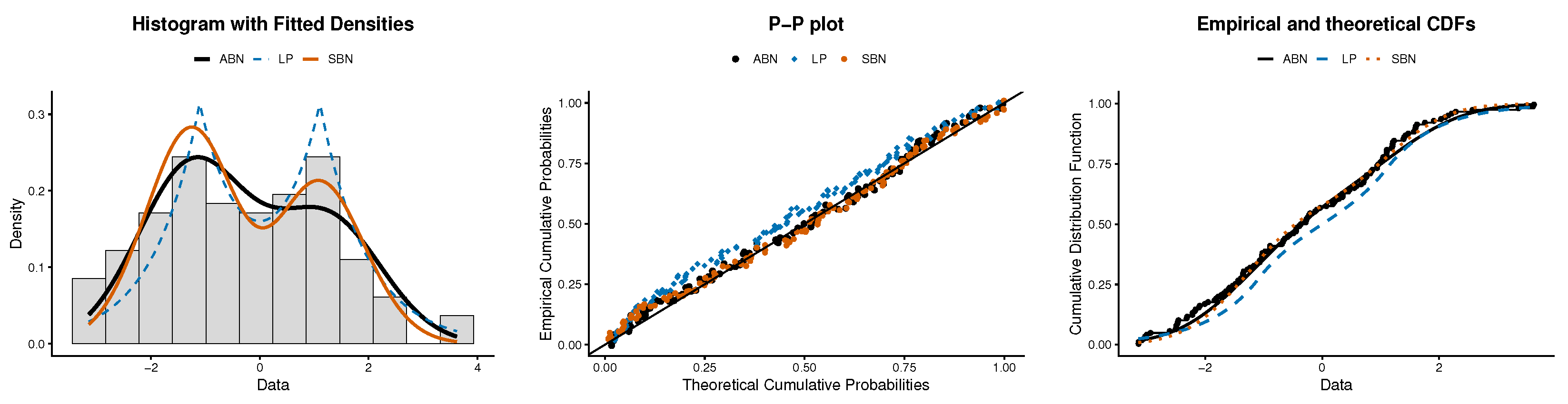
We support the observations with graphical diagnostics (Figure 3): histograms with fitted densities, P–P plots comparing empirical and theoretical probabilities, and empirical CDFs. Although all three models perform similarly, the ABN shows a clearer advantage in both the P–P and empirical CDF plots. The density plots indicate that ABN tracks the central mass and tail behavior more accurately than LP and SBN. While SBN captures the mode reasonably well and LP displays noticeable deviations, ABN consistently provides the best visual fit. These findings are in agreement with the AIC and BIC, confirming that ABN offers the best overall modeling performance on the DLDA30 dataset.

10.2. NIST Chemical Calibration Data

In this example, we use a dataset that consists of actual measurement deviations from chemical calibration data provided by the National Institute of Standards and Technology (NIST) https://www.itl.nist.gov/div898/handbook (accessed on 12 December 2025). These observations represent repeated analytical measurements of a certified reference material conducted with a high-precision spectrophotometric instrument. Each value corresponds to the deviation from the actual reference concentration, including both negative and positive deviations. These chemical measurement deviation data are widely used in analytical chemistry and metrology to assess instrument accuracy, calibration stability, and uncertainty estimates [30,31]. Due to their empirical characteristics, which are usually unimodal, leptokurtic, and occasionally slightly distorted, these data provide an ideal benchmark for evaluating flexible distributions. The 30 observations used in this paper were randomly sampled from the original NIST chemical calibration database and constitute a representative subset suitable for distributional adjustment, error modeling, and reliability analysis. The dataset consists of 30 measurement deviations, taking the following values: –2.05, –1.88, –1.60, –1.42, –1.25, –1.05, –0.85, –0.70, –0.52, –0.38, –0.25, –0.12, 0.00, 0.08, 0.15, 0.28, 0.40, 0.55, 0.70, 0.88, 1.05, 1.22, 1.40, 1.58, 1.80, 1.95, 2.12, 2.28, 2.42, and 2.55.

In this example, we compare the ABN model with the well-known skew-normal (SN) and asymmetric Laplace (AL) distributions since their ranges include both positive and negative values. The results in

Table 3. Summary of MLEs, goodness-of-fit statistics, and information criteria for the ABN, SN, and AL distributions fitted to the NIST chemical calibration data.

Model	MLEs	K-S	AD	CvM	AIC	BIC
ABN	$\widehat{\alpha }=0.2668\left(0.1560\right)$ $\widehat{\lambda }=0.9322\left(0.1855\right)$	0.0768 (0.9886)	0.2187 (0.9740)	0.0227 (0.9945)	104.8753	107.6777
SN	$\widehat{\lambda }=0.0516\left(21.1520\right)$ $\widehat{\mu }=0.2573\left(0.8852\right)$ $\widehat{\sigma }=1.3145\left(20.2127\right)$	0.0715 (0.9950)	0.2222 (0.9850)	0.0260 (0.9887)	107.4933	111.6969
AL	$\widehat{\mu }=0.0798\left(0.0347\right)$ $\widehat{\sigma }=1.0870\left(0.1990\right)$ $\widehat{\kappa }=1.1122\left(0.1455\right)$	0.0855 (0.9673)	0.3941 (0.8660)	0.0503 (0.8778)	112.9298	117.1334

show that all models fit the data well. The ABN model exhibits the smallest AIC and BIC values, indicating the best fit. Additionally, the standard errors of the parameter estimates are relatively small.

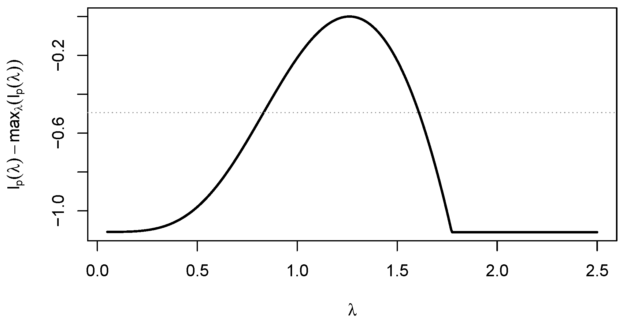
Remark 18.

The extremely large standard errors observed for the SN model estimates ($\widehat{\lambda }$ and $\widehat{\sigma }$) are symptomatic of the well-known singularity of the skew-normal Fisher information matrix when the shape parameter is near zero (symmetry). The ABN model, in this case, provides a more stable estimation. This weak curvature regime is illustrated in Figure 4 via the relative profile log-likelihood for the SN shape parameter λ, showing the characteristic flattening when λ is near 0.

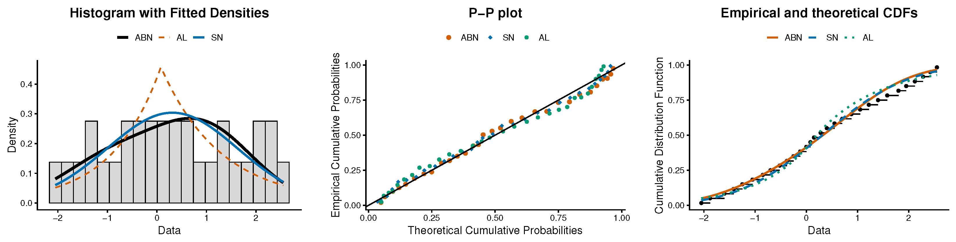
In this case, the superiority of the ABN distribution over the SN and AL models is evident for the NIST chemical calibration data. The ABN model yields the smallest AIC and BIC values, and all goodness-of-fit statistics consistently indicate that this data set can be adequately modeled by $ABN(\widehat{\lambda }=0.9322,\widehat{\alpha }=0.2668)$. This conclusion is further supported by the graphical analyzes in Figure 5. While the SBN model aligns reasonably well with the empirical histogram around the modal region, the ABN model captures the central mass and overall shape of the data more accurately. In the PP plot and empirical CDF comparison, the ABN curve remains closest to the reference line across the full range of the distribution, demonstrating a more consistent fit than its competitors. Taken together, these results confirm that the ABN model is the most appropriate choice for modeling the NIST chemical calibration dataset.

10.3. Residential Customers Data (Regression Analysis)

The ABN distribution is extended to a linear regression setting defined by:

$$y_i={\mathbf{x}}_i\mathit{\beta }+{ϵ}_i,i=1,\dots ,n.$$

(21)

Instead of the traditional assumption that errors follow a normal distribution (${ϵ}_i\sim N(0,{\sigma }^2)$), we propose that the error terms ${ϵ}_i$ follow the $ABN(\alpha ,\lambda )$ distribution. By ensuring $\mathbb{E}\left({ϵ}_i\right)=0$ and defining the variance as $\mathrm{Var}\left({ϵ}_i\right)=1+{\lambda }^2\left(1-{\alpha }^2\right)$, we obtain the expected structure of the regression model as: $\mathbb{E}\left(Y_i\right)={\mathbf{x}}_i\mathit{\beta }$. For this illustration, the residential customer data provided by Montgomery et al. [32] is utilized.

Table 4. MLEs for the residential customers data, and the corresponding standard errors (in parentheses) and AIC and BIC values.

Estimates	SN	N	TN	ABN
${\widehat{\beta }}_0$	$-0.83130$	$-0.83130$	$-0.83130$	$0.02287$
	$\left(0.3032\right)$	$\left(0.28000\right)$	$\left(0.31037\right)$	$\left(0.48692\right)$
${\widehat{\beta }}_1$	$0.00021$	$0.00368$	$0.00368$	$0.00337$
	($0.00368$)	$\left(0.00021\right)$	$\left(0.00023\right)$	$\left(0.00027\right)$
$\widehat{\alpha }$	−1.16 × 10−8			$-0.44427$
	(0.14583)			$\left(0.19566\right)$
$\widehat{\lambda }$			$0.50000$	$1.23266$
			$\left(0.30883\right)$	$\left(0.21162\right)$
AIC	230.2735	228.2735	217.7638	206.5130
BIC	236.1844	232.2141	223.6747	214.3942

presents the MLEs along with their corresponding standard errors, as well as the AIC and BIC values for the SN, N, TN, and ABN regression models. When evaluating model performance, it is evident that the ABN model significantly outperforms the competitor models. The ABN model yields the lowest AIC ($206.5130$) and BIC ($214.3942$) values, indicating a superior goodness-of-fit compared to the normal (AIC = $228.2735$), skew-normal (AIC = $230.2735$), and two-piece normal (AIC = $217.7638$) models.

Specifically, the substantial reduction in AIC and BIC values suggests that the ABN distribution captures the underlying structure of the residential customer data much more effectively than the standard or other extended normal distributions. Furthermore, the standard errors for the ABN estimates are within reasonable limits, confirming the stability of the parameter estimation.

To detect potential outliers and assess model misspecification, the transformed martingale residuals are analyzed, denoted as $rM{T}_i$, as suggested by Barros et al. [33]. These residuals are defined by the transformation:

$$rM{T}_i=sgn\left(r{M}_i\right)\sqrt{-2\left[r{M}_i+{\kappa }_i\log ({\kappa }_i-r{M}_i)\right]},i=1,\dots ,n,$$

(22)

where $r{M}_i={\kappa }_i+\log \left(S(e_i;\widehat{\theta })\right)$ represents the martingale residual proposed by Ortega et al. [34]. Here, ${\kappa }_i\in \{0,1\}$ indicates the censoring status (0 for censored and 1 for uncensored observations), $sgn\left(·\right)$ is the sign function, and $S(e_i;\widehat{\theta })$ denotes the survival function evaluated at the standardized classical residuals $e_i$, with $\widehat{\theta }$ representing the MLE of the parameter vector $\theta$. To verify the validity of the model assumptions, the error distribution, and the goodness-of-fit, we constructed simulated envelopes based on diagnostic analysis techniques from the literature.

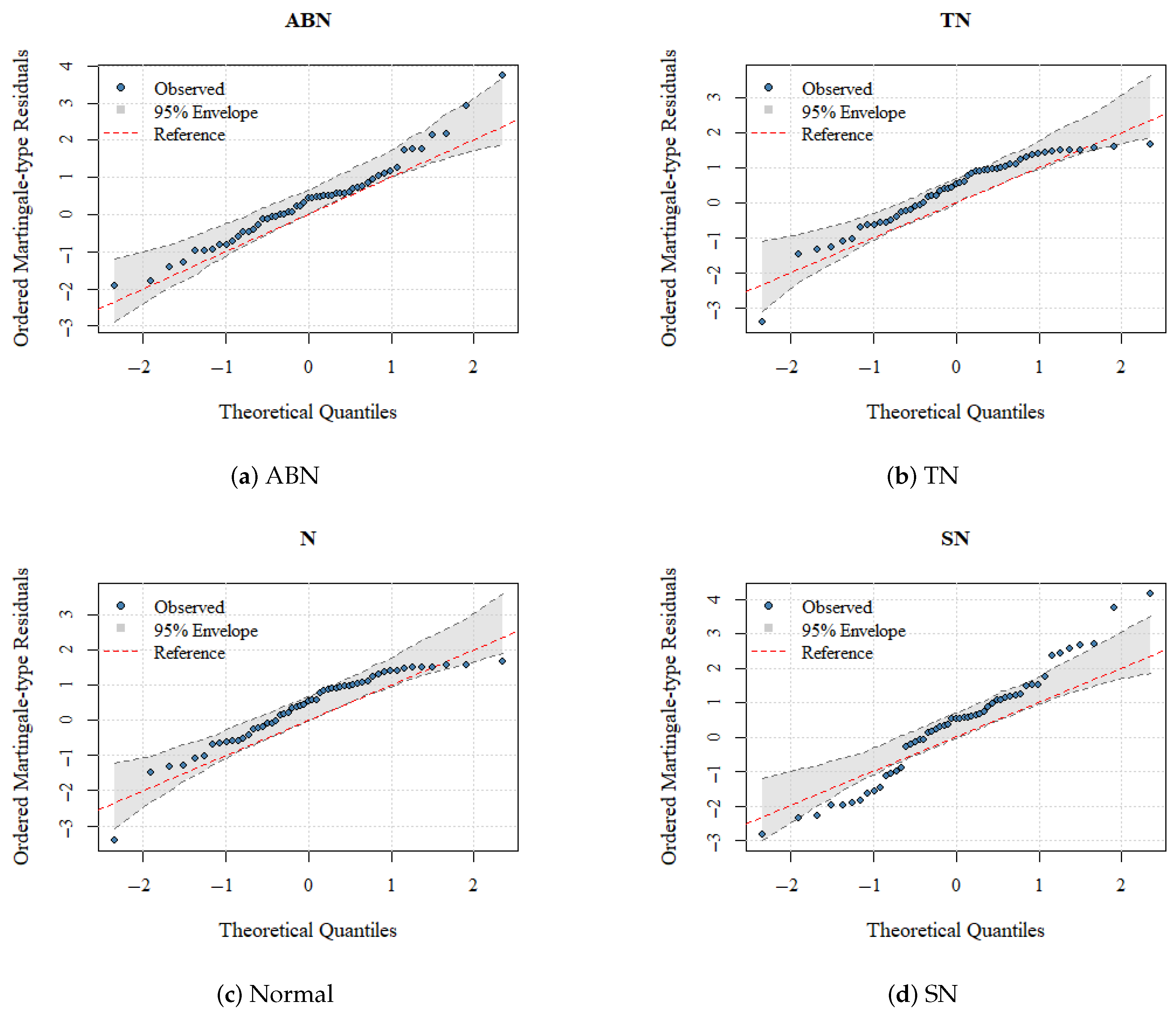
Figure 6 presents the Q-Q plots of the ordered martingale-type residuals for the ABN, N, SN, and TN regression models. For all models, the residuals are generally close to the reference line around the center, indicating an acceptable fit in the central region of the data. The ABN model shows the best overall performance. Most residuals closely follow the reference line and remain inside the 95% confidence envelope across the full range of theoretical quantiles. Only small deviations are observed in the extreme tails, suggesting that the ABN model captures skewness and tail behavior effectively.

The N and TN models display clearer departures from the reference line, especially in the lower and upper tails. Several points move away from the confidence envelope, indicating that these models have difficulty accommodating asymmetry and tail features in the data. The SN model improves the fit compared to the N and TN models by allowing skewness. However, noticeable deviations are still present in the tails, particularly for larger quantiles.

Overall, the residual diagnostics confirm that the ABN model provides the most adequate description of the data. Its residuals show the closest agreement with the theoretical quantiles, supporting the conclusion that the ABN regression model is preferable among the considered alternatives.

11. Discussion and Conclusions

This paper introduces the ABN distribution, a parsimonious two-parameter family designed to model continuous data exhibiting skewness and unimodality or bimodality. Formulated as a constrained Gaussian mixture with symmetric locations, the ABN model circumvents the label-switching problem inherent in unconstrained mixtures and ensures parameter interpretability. We derived closed-form expressions for the probability density and cumulative distribution functions, provided a transparent stochastic representation based on a signed folded normal variable, and established clear analytical conditions distinguishing unimodal from bimodal regimes.

For statistical inference, we developed a maximum likelihood estimation framework implemented via a numerically stable block-coordinate quasi-Newton routine, initialized by the method of moments. While Monte Carlo experiments demonstrated accurate point estimation across representative parameter settings, we also highlighted that Hessian-based (Wald) standard errors can become unstable in the vicinity of the unimodal boundary ($\lambda \to 0$), where the Fisher information matrix becomes singular; thus, inference based on the likelihood function (for example, using profile likelihood) is recommended in weak separation regimes. Empirical applications, including chemical calibration deviations from the National Institute of Standards and Technology and a regression analysis with asymmetric errors, showed that the ABN model offers a competitive or superior fit relative to skew-normal, asymmetric Laplace, and standard mixture alternatives, consistently yielding favorable Akaike and Bayesian information criteria values.

Limitations of the current proposal include its Gaussian tail behavior, which may reduce robustness against extreme outliers and the aforementioned inferential challenges under weak component separation. Promising avenues for future research include the development of scale mixtures of ABN distributions to accommodate heavy tails, the extension to multivariate settings with structured covariance matrices, and the implementation of penalized likelihood or Bayesian approaches to stabilize inference near the boundary of the parameter space.