On the Use of the Meshless Material Point Method for Microelectronic Devices

Abstract

In this work, the Material Point Method (MPM) is reviewed for application in the microelectronics industry. Microelectronic processes often involve large deformations, evolving interfaces, multiphysics coupling, and complex geometries that challenge conventional mesh-based methods such as the finite element method (FEM). Meshless methods provide an alternative solution that avoids these issues. A comparison is made between Smoothed Particle Hydrodynamics (SPH), Element Free Galerkin (EFG), peridynamics, Radial Basis Function–Finite Difference (RBF-FD), and MPM, evaluated with respect to convergence, consistency and stability, boundary enforcement, adaptivity, coupling, and industrial applicability. Based on this assessment, MPM and its main variants (BSMPM, GIMP, CPDI, and TLMPM) are examined in depth. The method’s ability to address large deformations, moving interfaces, contact, history-dependent material behavior, and multiphysics interactions is examined. The underfill process is used as a representative use case to illustrate challenges such as free surface flow, void formation, thermomechanical coupling, and residual stress. Overall, MPM shows strong potential, although further benchmarking and validation are required for widespread industrial adoption.

1. Introduction

Meshless methods are gaining in popularity as a promising alternative to traditional simulation methods. By avoiding a fixed mesh and instead relying on particles or scattered nodes to represent the domain, meshless methods are more suitable for handling large deformations, complex geometries, and moving interfaces. Within meshless methods, several variants exist. In this paper, we focus on the Material Point Method (MPM). In microelectronics, significant displacements and evolving flow fronts can occur during production and operation, such as wire sweep during encapsulation or void formation in the underfill. Accurately capturing these phenomena is critical for reliability assessment and design optimization. Despite this, meshless methods have not seen much use in the field. This limited adoption can be attributed to several factors. Conventional mesh-based methods benefit from decades of development, extensive verification and validation, and widespread availability in commercial simulation software commonly used in industry. In contrast, meshless methods often require additional algorithms for boundary enforcement and stabilization techniques. Nevertheless, ongoing methodological developments and increasing computational capabilities are gradually improving their industrial viability. The increasing miniaturization and heterogeneous integration of microelectronics have made microelectronic systems more powerful, but also more susceptible to failure due to mechanical, thermal, and fluidic effects. During both fabrication and operation, these electronic devices are subjected to complex physical processes, such as encapsulation, thermal cycling, and interface delamination. Predicting the effects of these physical processes requires accurate and robust simulation tools. However, it is non-trivial to simulate such complex multiphysical phenomena. The inherent multiphysics coupling, the presence of material interfaces, the occurrence of large deformations, and the geometric complexity of thin structures with high aspect ratios all pose significant challenges for conventional numerical methods.

Mesh-based techniques, such as the Finite Element Method [1] (FEM) and Finite Volume Method [2] (FVM), have long been the standard in microelectronic simulation. While proven effective in many domains, these methods often struggle when applied to problems involving complex geometries, evolving boundaries, large deformations, or topological changes, which results in severe mesh distortions and low element quality. In particular, creating a mesh of sufficient quality leads to long preprocessing times. Remeshing strategies can introduce numerical diffusion and loss of accuracy while increasing computational demands. Additionally, enforcing boundary conditions across complex interfaces remains challenging. These limitations can become problematic when simulating the capillary underfill process, overmoulding encapsulation, crack propagation in the solder bump, and interface delamination.

Of course, development of mesh-based methods has not stood still, and many improvements have been made over the years to mitigate these problems. The Spectral Element Method (SEM) is a FEM formulation that uses higher order basis functions to achieve better accuracy [3]. While SEM can handle larger mesh distortions than FEM [4,5], the problem is not eliminated completely. The extended finite element (XFEM) was introduced to address discontinuities such as fractures. XFEM uses an additional degree of freedom to approximate the discontinuity, eliminating the need for remeshing to describe the evolving fracture [6]. However, XFEM requires additional techniques to track crack propagation throughout the mesh, or unstable results will arise. The necessity of tracking algorithms is seen as one of the major weak points of XFEM [7]. Convergence is still an issue, in part due to deformed elements [8]. Arbitrary Lagrangian–Eulerian (ALE) methods, such as ALE-FEM, use a moving mesh to keep the mesh aligned with the evolving boundaries [9]. This makes it well-suited for tracking the interface in Fluid-Structure Interactions [10] (FSI). The ALE framework reduces the effects of distortions [11], but maintaining mesh quality while continuously reconstructing the mesh is both error-prone and resource-intensive [12].

Meshless methods have emerged as a way to avoid the problems inherent to using a mesh. For example, the Material Point Method (MPM) has been used to model high velocity impacts [13] and the morphology of the debris cloud [14]. In these problems, large deformations, complex geometries, and evolving boundaries can be captured without the need for remeshing. Nevertheless, meshless methods are not immune to numerical errors arising from irregular node or particle distributions. In fluid mechanics simulation, particles can cluster along streamlines [15], which can reduce accuracy and stability. Mitigation techniques are available to address these effects, such as the particle-shifting technique [16] and the $\delta$-correction [17]. This highlights that meshless methods introduce different numerical challenges compared to mesh-based approaches, while often providing improved robustness in problems involving large deformation and evolving geometries. It is therefore important to choose a suitable method for the desired application. Throughout the years, different methods have been proposed, each with their own advantages and disadvantages. Which method is best suited to tackle the problems encountered during the design, manufacturing and use of microelectronics remains an open question. Any method must be robust under large deformations while also accurately capturing interface behavior, effectively coupling multiphysics, and remaining computationally efficient in three dimensions. The different methods share some commonalities; they deal well with large deformation, complex geometries, and do not require remeshing, but they differ greatly in other areas. For instance, Smoothed Particle Hydrodynamics (SPH) exclusively uses purely Lagrangian particles to discretize the computational domain, while the Material Point Method (MPM) uses a hybrid approach—Lagrangian material points together with an Eulerian computational grid. The available meshless methods will be compared on five different aspects: numerical performance, boundary enforcement, adaptivity, integrability, and industrial applicability. From this evaluation, MPM is selected and its formulation is explained in depth, and an overview of its commonly used variants is provided. The advantages of MPM for microelectronic simulations are reviewed. Finally, the underfill process is chosen to demonstrate the capabilities of MPM for the microelectronics field.

While several reviews discuss the theoretical and computational development of the Material Point Method [18,19], an assessment of its suitability for microelectronics simulation is currently missing. This review aims to bridge this gap by evaluating MPM and related meshless methods specifically within the context of microelectronics applications, demonstrating the advantages of MPM over other meshless techniques, and outline future directions that could further enhance its role in the field.

2. Overview of Meshless Methods

Meshless methods have emerged as a powerful alternative when traditional mesh-based methods struggle to find a solution. Unlike FEM or FVM, which rely on a mesh to discretize the computational domain, meshless methods use a set of scattered points to represent the geometry, store variables, and perform numerical computations. This fundamental difference offers a range of advantages in problems where the domain undergoes large deformations or topological changes, or where remeshing would be required. As for mesh-based discretizations, there are various meshless methods with fundamentally different approaches. Five different meshless methods are discussed here: Smoothed Particle Hydrodynamics (SPH), Element-Free Galerkin (EFG), peridynamics, Radial Basis Function Finite Difference (RBF-FD), and the Material Point Method (MPM). They are compared in five main areas: (1) ensuring convergence, consistency, and stability, (2) enforcing boundaries, (3) enabling adaptivity, (4) coupling with other methods, and (5) demonstrating industrial applicability. These five areas, dubbed the grand challenges by some [20], allow for a good comparison between the discussed methods. While all criteria are treated equally in the comparison table, their relative importance depends on what is being simulated. Convergence, consistency, and boundary enforcement are directly related to accuracy, adaptivity affects computational efficiency while maintaining accuracy, coupling allows leveraging complementary methods in different subdomains, and industrial applicability reflects the practical utility and adoption of the method. An overview of how each method performs across these five key areas is provided in

Table 1. A comparison of different meshless methods.

Method	Convergence, Consistency, Stability	Boundary Enforcement	Adaptivity	Coupling with Other Methods	Industrial Applicability
SPH	Has been shown, but formal analysis difficult	No fixed point for boundary enforcement	APR implemented, but leads to errors	SPH-FEM, SPH-DEM	Currently too inefficient
EFG	Formal analysis difficult	Requires additional methods	Strain gradients, h-adaptivity	FEM	Available in commercial software, but not great for multiphysics
Peridynamics	Has been shown, but formal analysis difficult	Requires additional methods, prone to errors	Dual Horizon peridynamics	FEM and SPH	For fractures only, but needs improved parallel computing
RBF-FD	Ill-conditioning a problem, but can be mitigated	Dependent on number of internal and boundary nodes, and the stencil size	Unstructured nodes, TPS	FEM and FDM	Good for multiphysics
MPM	Has been shown, but formal analysis difficult	Easy on the grid, on particles similar to SPH	Unstructured background grid, AMR, THB-MPM	MPM-FEM, MPM-DEM, SEM-MPM, SPH-FEM	Established in graphics industry, shows promise for many applications.

.

The oldest method is SPH, originally developed for astrophysics [21], which utilizes Lagrangian particles to discretize the domain. It has gained popularity in fluid dynamics and impact modeling, particularly where large deformations and free surfaces occur. Ensuring convergence, consistency, and stability is an important topic for any numerical scheme, and SPH is no different. A problem particular to SPH is that its purely Lagrangian particles make formal analysis difficult. Boundary enforcement is problematic in SPH due to its meshless and Lagrangian nature; in short, SPH does not have fixed points to impose the boundary on. This leads to worries for conservation, stability, and solid wall boundaries for complex geometries. Adaptivity refers to the ability of a numerical scheme to use a different spatial resolutions throughout a domain. In mesh-based methods, this would mean a finer mesh in some parts of the domain and a coarser mesh in other parts. In SPH, almost all existing codes use a uniform resolution, reducing efficiency and ability to simulate multiscale problems. Some efforts have been made, such as an Adaptive Particle Refinement [22] (APR), but increased errors and robustness remain a challenge. Coupling SPH to other methods, mainly FEM or DEM, is possible, but it requires complex coupling algorithms, again due to the fully Lagrangian nature of SPH. The benefits of a coupled solver are impressive enough that much work has gone into developing SPH-FEM [23] and SPH-DEM [24]. The industry’s resistance is not unique to SPH, but a challenge to all meshless methods. Apart from some novel problems, meshless methods will have to replace existing mesh-based methods well established in industry. This requires meshless methods to outperform existing methods in efficiency and the ability to simulate complex multiphysics problems. Unfortunately, SPH is inherently more computationally expensive, but accelerating it on CPUs or GPUs and improving convergence can reduce simulation times.

The Element-Free Galerkin [25] (EFG) method uses Moving Least Squares [26] (MLS) interpolation with a background grid structure to approximate the solution. It provides accurate results even for steep local field gradients [27], making it attractive for solid mechanics problems. It can be implemented in a fully Lagrangian, fully Eulerian, or an Arbitrary Lagrangian–Eulerian (ALE) framework, allowing for an optimal description for different physics. Nonetheless, numerical analysis is difficult, so it is hard to show proper convergence, consistency and stability. Boundary enforcement always requires additional methods such as a penalty method [28,29] or Lagrange multipliers [30,31]. The method is able to be locally refined based on some criteria [32,33,34]. EFG has been frequently used in conjunction with FEM [35,36,37], but has not been used together with other methods. Work with EFG has primarily remained in the academic sphere, but actual use in industry is getting closer. An EFG formulation is implemented in ANSYS LSDYNA EFG, which makes EFG one of the few methods that has been implemented in commercial software. Multiphysics coupling is possible in EFG [38,39], but is significantly more difficult when moving interfaces (e.g., a fluid–structure interface) are involved [27]. It is being held back by accuracy, efficiency, and ease of boundary implementation.

Peridynamics was developed for modeling discontinuities and multiscale analysis of materials. It discretizes the domain with a point cloud, where the points interact with other points within a certain horizon. This makes peridynamics non-local; it does not exclusively interact with its direct neighbors. It is unusual that peridynamics uses integro-differential equations instead of partial differential equations solved by most methods. Its non-local nature and integro-differential formulations make formal analysis difficult, but in some cases, good convergence can be shown [40]. Peridynamics suffers from errors near boundaries and crack paths and requires additional methods to enforce boundary conditions [41]. External loads have to be implemented differently because the boundary traction does not appear in the equation of motion [42]. Dual-horizon peridynamics allows particles to have different horizons throughout the domain, making adaptivity relatively easy [43]. Other adaptivity methods are also available [44]. Peridynamics has been coupled with FEM [45] and SPH [46] for hydromechanical fractures. It is heading towards fracture analysis for industrial applications, but still needs to improve its efficiency by improving its parallel computing abilities [47].

The radial basis function-generated finite difference (RBF-FD) uses scattered node stencils to approximate the solution [48]. Regarding convergence, consistency, and stability, RBF-FD formulations commonly suffer from ill-conditioning, which can lead to instability and convergence problems [49]. There are ways to address ill-conditioning by using hybrid kernels at an increased computational cost [50]. For boundary enforcement, the error depends on the number of boundary nodes and internal nodes, and the stencil size [51]. In terms of adaptivity, the unstructured node distribution naturally accommodates local refinement, which is beneficial for resolving localized phenomena such as sharp gradients, moving interfaces, or evolving discontinuities, while maintaining computational efficiency. More advanced refinement schemes through Thin Plane Spline (TPS) radial basis functions [52] have also been proposed. RBF-FD has been coupled to FEM [53] and the Finite Difference Method (FDM) [54]. The method has shown promise for solving multiphysics problems, for instance in modeling the thermo-elasto-plastic physics in the continuous casting of steel [55]. Additionally, it has been used in the geosciences [56], and even economics [57].

The Material Point Method (MPM) stands out among meshless methods due to its hybrid nature. In MPM, material is represented by a collection of Lagrangian particles that carry state variables such as mass, momentum, and stress. These particles interact via a background Eulerian grid, which is used temporarily to solve the governing equations. After each time step, the grid is reset, avoiding issues with mesh distortion. This dual representation allows MPM to capture large deformations and dynamic contact naturally while maintaining the accuracy and stability of a structured solver. Formal analysis is difficult, but proper convergence has been shown in some cases [19,58]. Spurious oscillations have long plagued MPM, but advances such as B-spline MPM, CPDI, and stabilization techniques have greatly reduced instabilities. Applying boundary conditions is easier compared to pure particle methods, but still harder than FEM, because of the similarities between the background grid and a conventional mesh. Adaptivity techniques from mesh-based methods can be used without much alteration. Adaptive Mesh Refinement (AMR) has been applied to MPM for hypersonic aeroelasticity problems [59,60]. Another option is to use Truncated Hierarchical B-splines as done in [61]. MPM is well suited to couple to other numerical methods when beneficial. It has therefore often been coupled to FEM and DEM, but to more advanced mesh-based methods such as SEM-MPM [62]. A coupled MPM-SPH solver has even been proposed, because it would make it easier to couple SPH with a mesh-based method [63]. The larger number of demonstrated couplings does not necessarily indicate superiority over other meshless methods, but reflects the flexibility and compatibility of the MPM framework. Such coupled approaches allow different numerical methods to be employed in different regions of a computational domain, enabling the selection of the most appropriate discretization for each physical process. This is particularly attractive for multiphysics simulations in microelectronics, where mechanical, thermal, and fluid phenomena may coexist. Notably, MPM has been used for computer graphics applications in movies such as Frozen, Big Hero 6, and Zootopia [64]. These applications primarily focus on visually realistic animation rather than physically predictive simulation. Nevertheless, developments originating from computer graphics have significantly advanced the MPM framework. For instance, the widely used PIC-FLIP scheme was introduced by Stomakhin et al. [65], originally developed to improve the animation of snow. Such developments have subsequently contributed to improved numerical stability, efficiency, and robustness, which are also valuable for microelectronics applications. While adoption in computer graphics does not directly validate MPM for engineering applications, it demonstrates the scalability, algorithmic maturity, and parallel performance of MPM implementations at large problem sizes. In an engineering context, MPM has been used for additive manufacturing [66], explosive welding [67], avalanches, dam-breaks, machining [68,69,70], impact mechanics [71,72,73], soft tissue mechanics [74,75], composites [76], forging [77,78], soft robotics [79], and sintering [80]. Additionally, MPM is generally more efficient than SPH, because it does not require the computationally expensive particle search algorithms necessary in SPH. Parallelizing MPM is made much easier due to the Eulerian grid, and is done in many of the open-source MPM codes available, such as Uintah [81], Karamelo [82], CB-Geo [83], and Taichi MPM [84]. MPM is, therefore, not only able to handle the complex multiphysics encountered in many industrial problems, but also able to simulate them with good efficiency.

3. The Material Point Method

The Material Point Method has not seen any use in the microelectronics field, so we expect some readers may be unfamiliar with the method. Therefore, in this section, we provide an explanation of MPM. The hybrid Lagrangian–Eulerian description and its advantages are discussed. Then, the computational procedure MPM uses to achieve this hybrid approach is detailed.

3.1. Hybrid Lagrangian–Eulerian Description

To explain the benefits of employing a hybrid Lagrangian–Eulerian description (i.e., MPM), the advantages and disadvantages of both must first be examined individually. Start with a purely Lagrangian description, where the integration points move with the displacement field. The advantage of this is that it can capture complex geometries, can track deformation explicitly over time to more accurately capture morphological changes, and can capture and track interfaces and free surfaces. The disadvantage of the Lagrangian description is that the moving integration points have to be tracked, increasing computational cost. Additionally, the shape functions need to be continually reconstructed, slowing the simulation down further. Moreover, when simulating fluids, Lagrangian particles tend to move along streamlines leading to particle clustering and increased quadrature errors, while in other regions, it becomes too sparse, decreasing resolution and accuracy [15].

The Eulerian description is, in some sense, the opposite of the Lagrangian. The integration points are fixed in space and the displacement field is free to move around in the computational space. The advantage of this approach is that the shape function does not have to be reconstructed and the imposition of the boundary conditions can be applied explicitly. Furthermore, it has a simpler data structure with regular and predictable memory access patterns, making parallelization easier and increasing efficiency. However, the disadvantages are that it requires additional techniques to track interfaces and free surfaces, and it cannot capture the details in morphological changes. Additionally, the Eulerian approach is not suited for splitting and merging the computational domain, such as in fractures or anti-fractures.

One notices that the two descriptions are often complementary. The Eulerian is more efficient, easier to parallelize, and has easier implementation of the boundary conditions, but has trouble dealing with interfaces, free surfaces, and morphological changes. While the Lagrangian is useful for tracking interfaces, free surfaces, boundaries, and morphological changes, it is harder to parallelize, and has a higher computational cost and more complex boundary causality. Therefore, the hybrid approach used in MPM is able to achieve the best of both worlds.

3.2. Computational Procedure

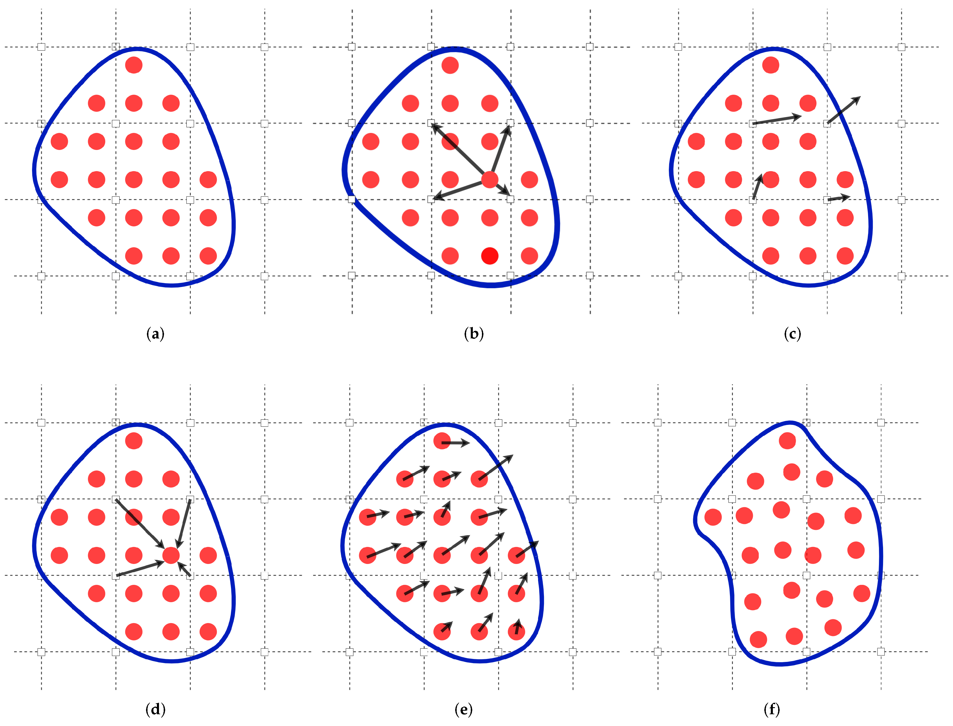
The hybrid Lagrangian–Eulerian description used in MPM is achieved by a set of pure Lagrangian points and Eulerian nodes on the computation grid. The domain is discretized using the grid and $n_p$ points, as shown in Figure 1a. The material points contain mass $m_p$ ($p=1,2,...,n_p$), position ${\mathit{x}}_p^t$, velocity ${\mathit{v}}_p^t$, volume $V_p^t$, deformation gradient ${\mathit{F}}_p^t$, Cauchy stress tensor ${\mathsf{\sigma }}_p^t$, temperature $T_p^t$, and any other variable required for the constitutive model. Next, the type of shape function ${\varphi }_I$ and its gradient $\nabla {\varphi }_I$ must be decided upon. The choices are linear, quadratic B-splines, cubic B-splines, or Bernstein shape functions [85]. The relation between the material points and the grid nodes can then be determined, to map information to the nodes as in Figure 1b. The point masses can then be mapped to the nodes as

$$m_I^t={\Sigma }_p{\varphi }_I\left({\mathit{x}}_p^t\right)m_p,$$

(1)

where the subscript I and p indicate the nodal and point value, respectively. The nodal momentum is calculated as

$${\left(m\mathit{v}\right)}_I^t={\Sigma }_p{\varphi }_I\left({\mathit{x}}_p^t\right){\left(m\mathit{v}\right)}_p^t,$$

(2)

and the nodal force as

$${\mathit{f}}_I^t={\Sigma }_p[{\varphi }_I\left({\mathit{x}}_p^t\right)m_p\mathit{b}\left({\mathit{x}}_p^t\right)-V_p^t{\mathsf{\sigma }}_p^t\nabla {\varphi }_I\left({\mathit{x}}_p^t\right)],$$

(3)

where $\mathit{b}$ is the body force. The grid momentum can now be updated, as shown in Figure 1c. The updated momentum is found to be

$${\left(m\tilde{\mathit{v}}\right)}_I^{t+\Delta t}={\left(m\mathit{v}\right)}_I^t+\Delta t{\mathit{f}}_I^t,$$

(4)

where ${\tilde{\mathit{v}}}_I^{t+\Delta t}$ is a predictor velocity. The boundary conditions can now be applied on the grid, for example, on the boundary nodes $I_b$ as ${\left(m\tilde{\mathit{v}}\right)}_{I_b}^{t+\Delta t}=0$. The procedure here uses double mapping to find the grid velocity. Therefore, a predictor velocity is isolated with the nodal mass first as

$${\tilde{\mathit{v}}}_I^{t+\Delta t}={\left(m\tilde{\mathit{v}}\right)}^{t+\Delta t}/m_I^t.$$

(5)

The updated particle velocity can now be found using a combination of the Particle in Cell (PIC) method and the Fluid Implicit Particle (FLIP) method, first introduced by Stomakhin et al. [65] as

$${\mathit{v}}_p^{t+\Delta t}=(1-\alpha )\sum _I{\varphi }_I({\mathit{x}}_p^t){\tilde{\mathit{v}}}_I^{t+\Delta t}+\alpha ({\mathit{v}}_p^t\sum _I{\varphi }_I({\mathit{x}}_p^t)({\tilde{\mathit{v}}}_I^{t+\Delta t}-{\mathit{v}}_I^t)),$$

(6)

where $0\le \alpha \le 1$. The updated grid momenta ${\left(m\mathit{v}\right)}_I^{t+\Delta t}$ are recalculated using (2), but now with the updated particle velocities. The boundary conditions are reapplied on the grid, and the nodal velocities are again isolated as in (5). One notices the particle velocity has now been mapped to the grid twice, hence the name double mapping. The next step is to use the nodal velocities ${\mathit{v}}_I^{t+\Delta t}$ to calculate multiple particle variables, as in Figure 1d. Start with the gradient velocity, which is found as

$${\mathit{L}}_p^{t+\Delta t}={\Sigma }_I\nabla {\varphi }_I\left({\mathit{x}}_p^t\right){\mathit{v}}_I^{t+\Delta t},$$

(7)

which can be used to find the gradient deformation tensor with

$${\mathit{F}}_p^{t+\Delta t}=(\mathit{I}+{\mathit{L}}_p^{t+\Delta t}){\mathit{F}}_p^t.$$

(8)

The determinant is used to find the updated volume as

$$V_p^{t+\Delta t}=\det \left({\mathit{F}}_p^{t+\Delta t}\right)V_p^0.$$

(9)

Now, the particle stresses are updated using a constitutive model by

$${\mathsf{\sigma }}_p^{t+\Delta t}={\mathsf{\sigma }}_p^t+\Delta {\mathsf{\sigma }}_p.$$

(10)

The particles are moved to their new positions using

$${\mathit{x}}_p^{t+\Delta t}={\mathit{x}}_p^t+\Delta t{\Sigma }_I{\varphi }_I\left({\mathit{x}}_p^t\right){\mathit{v}}_I^{t+\Delta t},$$

(11)

as shown in Figure 1f. The grid is reset (i.e., $m_I^t=0$, ${\left(m\mathit{v}\right)}_I^t=0$, ${\mathit{f}}_I^t=0$) and the time is advanced by $t=t+\Delta t$. The procedure starts again from (1) until the end time is reached.

3.3. MPM Variants

The original MPM formulation used linear basis functions $\varphi$ based on the grid spacing h as

$${\varphi }_I\left(x\right)=\left\{\begin{array}{cc}1-{\displaystyle \frac{|x-x_I|}{h}},\hfill & \mathrm{if}|x-x_I| \le h,\hfill \\ 0,\hfill & \mathrm{else},\hfill \end{array}\right.$$

(12)

where $x_I$ is the nodal position. The gradient basis function $\nabla \varphi$ is

$$\nabla \varphi \left(x\right)=\left\{\begin{array}{cc}{\displaystyle \frac{1}{h}},\hfill & \mathrm{if}{x}_I-h\le x\le x_I,\hfill \\ -{\displaystyle \frac{1}{h}},\hfill & \mathrm{if}{x}_I\le x\le x_I+h.\hfill \\ 0,\hfill & \mathrm{else}\hfill \end{array}\right.$$

(13)

For higher dimensions, a tensor product of the 1D functions is taken as

$${\varphi }_I(x,y)={\varphi }_I\left(x\right){\varphi }_I\left(y\right),\nabla {\varphi }_I(x,y)=\left[\begin{array}{c}\nabla {\varphi }_I\left(x\right){\varphi }_I\left(y\right)\\ {\varphi }_I\left(x\right)\nabla {\varphi }_I\left(y\right)\end{array}\right].$$

(14)

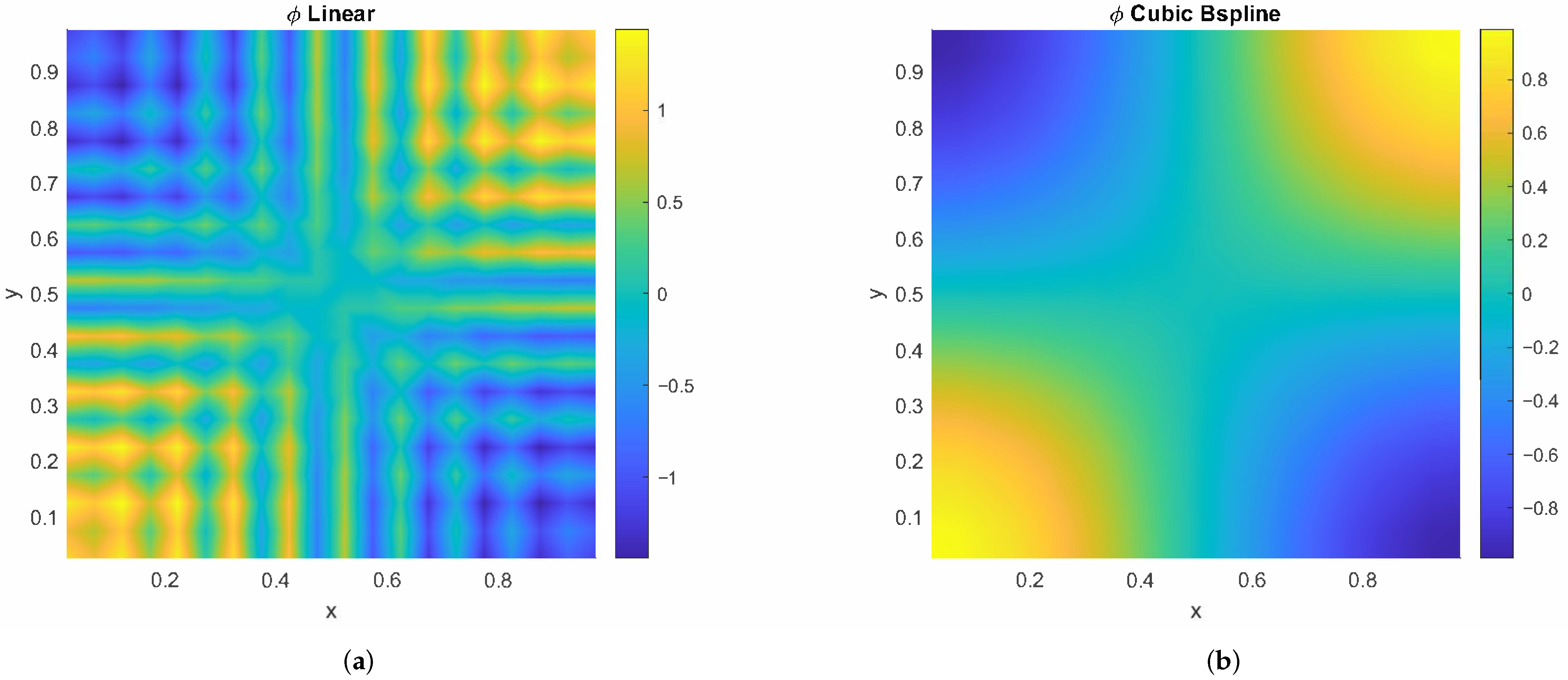
The original MPM formulation is, however, rarely used without additional stabilization techniques, because it is only $C^0$ continuous. The discontinuous derivative causes cell-crossing instabilities to occur when material points move into a new cell. This results in erroneous stress solutions and oscillations in the pressure term. To illustrate spurious oscillations in linear MPM, we consider the Helmholtz problem ${\nabla }^2\varphi -\varphi =-(2{\pi }^2+1)cos\left(\pi x\right)cos\left(\pi y\right)$ on the unit square $[0,1]\times [0,1]$, with Dirichlet boundary conditions prescribed from the exact solution ${\varphi }_{\mathrm{exact}}(x,y)=cos\left(\pi x\right)cos\left(\pi y\right)$. The resulting oscillations are clearly visible in Figure 2a. In order to mitigate the cell-crossing instabilities, improvements to MPM have been proposed. They include higher order basis functions, such as quadratic or cubic B-splines, the Generalized Improved Material Point (GIMP) method, Convected Particle Domain Interpolation (CPDI), and the Total Lagrangian Material Point Method (TLMPM).

The B-splines in MPM [86] are based on a knot vector $\mathrm{\Xi }=\{{\xi }_1,{\xi }_2,\dots ,{\xi }_{n+p+1}\}$ with knots ${\xi }_1\le {\xi }_2\le \dots \le {\xi }_{n+p+1}$, where n is the number of basis functions and p the polynomial degree. The zeroth order B-spline $p=0$ is given by

$${\varphi }_{i,p}\left(\xi \right)=\left\{\begin{array}{cc}1,\hfill & \mathrm{if}{\xi }_i\le \xi <{\xi }_{i+1},\hfill \\ 0,\hfill & \mathrm{else},\hfill \end{array}\right.$$

(15)

but is only used to determine higher order B-splines. For degrees $p\ge 1$, the basis functions are given by the recursion scheme [87]

$${\varphi }_{i,p}\left(\xi \right)={\displaystyle \frac{\xi -{\xi }_i}{{\xi }_{i+p}-{\xi }_i}}{\varphi }_{i,p-1}\left(\xi \right)+{\displaystyle \frac{{\xi }_{i+p+1}-\xi }{{\xi }_{i+p+1}-{\xi }_{i+1}}}{\varphi }_{i+1,p-1}\left(\xi \right),$$

(16)

where $i=1,2,\dots ,{\xi }_{n+p+1}$ and 0/0 is set to 0. The derivative of the B-spline function is provided by the recursive

$$\nabla {\varphi }_{i,p}\left(\xi \right)={\displaystyle \frac{p}{{\xi }_{i+p}-{\xi }_i}}{\varphi }_{i,p-1}\left(\xi \right)-{\displaystyle \frac{p}{{\xi }_{i+p+1}-{\xi }_{i+1}}}{\varphi }_{i+1,p-1}.$$

(17)

The most common B-splines used in MPM are quadratic ($p=2$) and cubic ($p=3$), which are at most $c^{p-1}$ continuous at a knot. For a knot with multiplicity k, (i.e., how many knot values ${\xi }_i$ are equal), the knot is $C^{p-k}$ continuous. Therefore, the B-splines are less sensitive to cell-crossing errors and oscillation (Figure 2b) as the original linear basis functions. However, some authors have noted MPM with higher order basis functions suffer more from early contact issues [88,89]. Early contact arises from the support domain of the basis functions relative to the background grid resolution. Interacting bodies or fluid fronts may detect contact once their support domains overlap, which can occur before the physical surfaces coincide. This effect is more pronounced for coarser grids or higher order basis functions, where the support radius is larger. Grid refinement reduces the magnitude of this effect by decreasing the effective support size, but does not eliminate it entirely. Early contact may be an issue in microelectronics, for instance when simulating the underfill flowing around the solder joints.

GIMP [90] uses linear basis functions, but treats the material points as small domains ${\Omega }_p$ inside $\Omega$. These domains are squares in 2D and cubes in 3D. With the inclusion of particle domains, the GIMP weighting function becomes

$${\varphi }_I^{GIMP}\left(\mathit{x}\right)={\displaystyle \frac{1}{V_p}}{\int }_{{\Omega }_p\cap \Omega }{\mathcal{X}}_p\left(\mathit{x}\right){\varphi }_I\left(\mathit{x}\right)d\mathit{x},$$

(18)

where ${\varphi }_I\left(\mathit{x}\right)$ is the linear shape function Equation (12). Although it is theoretically possible to use B-splines, to the best of the authors knowledge, this has not been implemented. The characteristic function ${\chi }_p\left(\mathit{x}\right)$ is

$${\mathcal{X}}_p\left(\mathit{x}\right)=\left\{\begin{array}{cc}1,\hfill & \mathrm{if}\mathit{x}\in {\Omega }_p,\hfill \\ 0,\hfill & \mathrm{if}\mathit{x}\notin {\Omega }_p,\hfill \end{array}\right.$$

(19)

which automatically satisfies the partition of unity ${\sum }_p{\mathcal{X}}_p\left(\mathit{x}\right)=1,\forall \mathit{x}$ at the initial state. The gradient weighting function for GIMP is given by

$$\nabla {\varphi }_I^{GIMP}={\displaystyle \frac{1}{V_p}}{\int }_{{\Omega }_p\cap \Omega }{\mathcal{X}}_p\left(\mathit{x}\right)\nabla {\varphi }_I\left(\mathit{x}\right)d\mathit{x}.$$

(20)

Unfortunately, GIMP has two major disadvantages. First, shear deformation and rigid body rotations cannot be computed because the particle domains remain rectangular throughout the simulation. This limitation may reduce physical relevance for microelectronic processes involving large shear, such as underfill flow around solder joints. Second, partition of unity is not guaranteed for the whole simulation time. Particle domain may overlap ${\sum }_p{\mathcal{X}}_p\left(\mathit{x}\right)=2$ or there may be discontinuities ${\sum }_p{\mathcal{X}}_p\left(\mathit{x}\right)=0$, introducing significant errors. Nevertheless, GIMP has significant advantages over the original MPM formulation and has thus seen frequent use.

The logical next step is to use variable particle domains, so the partition of unity can be preserved. Sadeghirad et al. [91,92] proposed the Convected Particle Domain Interpolation (CPDI), which uses quadrilaterals instead of rectangular particle domains. The shape functions for the second order CPDI are

$${\varphi }_I^{CPDI}={\displaystyle \frac{1}{V_p}}\sum _{\alpha =1}^4\left[{\int }_{{\Omega }_p}{N}_{\alpha }\left(\mathit{x}\right){\varphi }_I\left({\mathit{x}}_{\alpha }^p\right)d\Omega \right],$$

(21)

where $\alpha$ denotes the four corners of the quadrilateral, $N_{\alpha }$ the FEM shape function for a quadrilateral element, and ${\varphi }_I\left({\mathit{x}}_{\alpha }^p\right)$ the standard MPM shape functions to interpolate particle position ${\mathit{x}}_p$ to corner ${\mathit{x}}_{\alpha }$. Usually, the linear shape function Equation (12) is used, but recently, the B-splines have been implemented [93]. The gradient shape function for CPDI is given as

$$\nabla {\varphi }_I^{CPDI}={\displaystyle \frac{1}{V_p}}\sum _{\alpha =1}^4\left[{\int }_{{\Omega }_p}\nabla N_{\alpha }\left(\mathit{x}\right){\varphi }_I\left({\mathit{x}}_{\alpha }^p\right)d\Omega \right].$$

(22)

Despite the advantages over GIMP, there are some problems associated with CPDI. In highly distorted cases, a material point can pass through another without interacting. This may affect simulations involving extreme deformation or thin material regions. It can be resolved by particle splitting, that is locally increasing the particles per cell [94].

The last variant of MPM to be discussed here is the Total Lagrangian Material Point Method (TLMPM), originally proposed by Renaud et al. [95] and later developed by De Vaucorbeil [96]. In TLMPM, the stresses and strain are determined with respect to the reference configuration. This eliminates any problems with cell-crossing instabilities or numerical fracture. Currently, linear, B-splines, and Bernstein basis functions have been implemented in TLMPM, allowing for accurate and stable simulations. However, when spatial coordinates are required (e.g., contact), the material reference frame needs to be mapped to the spatial frame. Contact now demands additional algorithms to satisfy the non-penetration condition [97].

4. The Material Point Method for Microelectronics

The Material Point Method has several advantages which make it attractive for simulating microelectronic systems. Many processes in microelectronics involve complex, transient phenomena such as large material deformations, evolving interfaces, and strongly coupled multiphysics interactions, which pose significant challenges for conventional mesh-based methods. MPM provides a flexible and robust framework for addressing these challenges, but has not seen much use in microelectronics.

Table 2. The topic addressed in MPM literature from different research groups.

Group	MPM Variant	Physics	Interfaces & Boundaries	Contact Algorithm	Application
Soga [98,99,100]	BSMPM, TLMPM	Fluid, Solid, FSI	Free surface	Standard MPM contact	Numerical, geomechanical
Lian [66,101,102]	MPM, MPM-FEM	Thermo-FSI	Free surface	Hertz	Additive manufacturing
Molinos [100,103,104,105]	LME-MPM, TLMPM	Solid	Fractures	Standard MPM contact	Numerical
Qian [106,107,108,109,110]	BSMPM, LESCM	Fluid, FSI	Free surface	Standard MPM contact	Offshore
Pei Zhang [111,112,113,114,115]	GIMP, MPM-DEM	Fluid-particle, FSI	Free surface, slip-boundary	Contact force with ghost DEM particle	Geomechanical
Sang [89,116,117,118]	GIMP, BSMPM, MPM-FDM	Solid, particle	Free surface	Point-to-point, point-to-segment, penalty method	Geomechanics
Sun [119,120,121,122,123]	BSMPM	FSI	Free surface, slip boundary	Lagrange multipliers with Greville abscissa	Geomechanical, numerical
Moutsanidis [58,124,125,126,127]	BSMPM, TLMPM	Solid, fluid	Free surface	Velocity discontinuity	Numerical
Tran [128,129,130,131]	GIMP, ICE-MPM	Fluid, FSI, Thermal	Free surface	Coulomb	Geomechanical
Vaucorbeil [18,82,96,97,132,133,134,135]	TLMPM	Solid	Fracture	Particle-to-particle	Numerical

shows that it is a common topic in geomechanical applications and studies on numerical improvement (i.e., improving the method without a specific application in mind). The following paragraphs discuss the key advantages of MPM in the context of microelectronic applications.

• Robustness in the presence of large deformations

Many processes in microelectronics involve materials undergoing large deformations, including flow during encapsulation, solder reflow, and displacements during manufacturing and operation due to thermo-mechanical effects. Mesh-based methods often suffer from a loss of accuracy in such regimes due to mesh distortions and frequent remeshing. One of the most significant benefits of MPM is its robustness in the presence of large deformations. Since the computational grid is reset each step, MPM avoids mesh distortion and numerical instability typical of mesh-based methods. This is especially relevant for processes such as encapsulation, where the wire sweep causes significant mesh distortion, or crack propagation, where sudden discontinuities appear. However, the traditional MPM algorithm suffers from cell-crossing instabilities. While its variants discussed in Section 3.3 mostly resolve these instabilities, they come at an increase in computational cost because of the increased particle support domain. Nevertheless, these variants remain widely used in practice, including in the studies summarized in Table 2. Additionally, if the particle density is not sufficient, numerical fracture may occur. This is when the distance between material points can exceed the particle support domain. It can be mitigated by increasing the particle domain, for example, by using BSMPM. In extreme cases, it will require particle redistribution. TLMPM was developed in part to resolve the problem of numerical fracture.

• History-Dependent Behavior

Materials and processes encountered in microelectronics exhibit strongly history-dependent behavior, such as plastic deformation, viscoelasticity, damage evolution, and temperature dependent material response. Accurate simulation of these phenomena requires the consistent tracking of internal state variables over time. Storing all material properties on the material points enables the tracking of history-dependent variables such as stress, plastic strain, temperature, and damage [132]. This allows for highly localized and physically consistent modeling of material behavior, which is critical in devices where failure often initiates in small regions due to stress concentration or thermal gradients and CTE mismatch. However, one should be careful with the storage and computational overhead required for tracking all these historical variables. The modeling of a thermomechanical failure may include storing temperature history, plastic strain, and damage variables for each particle. For high-resolution simulations, this can have significant memory requirements.

• Moving Interfaces and Evolving Boundaries

In addition, MPM naturally accommodates moving interfaces and evolving boundaries, such as free surfaces in fluid mechanics, without requiring remeshing or complex interface elements. This is reflected in the research summarized in Table 2, where free-surface problems are commonly addressed. MPM has a long history with modeling fluid mechanics. Originally based on PIC, which was intended for fluids, modeling fluids with MPM goes back to its roots. There are, however, still issues limiting the application of MPM for fluids, so it is a popular topic of research, as shown in Table 2. Spurious oscillations present in the original MPM can cause instabilities and errors, so a lot of recent work has been done to improve the performance of MPM when simulating fluids. While some of the problems of the original MPM implementation can be mitigated with improved variants, such as GIMP or CPDI, and more advanced basis functions (e.g., B-spline [136]), there are authors working on improving the flow properties themselves. Stabilization techniques are implemented to reduce the pressure oscillations, such as a polynomial pressure projection [137], assumed gradient method with volumetric averaging [138], the Variational Multiscale (VMS) method [98], operator splitting with hourglass dampening [139], and fractional-step [99], which are employed to stabilize the pressure in MPM. It should be noted that while these stabilization techniques improve the results, they can significantly increase the computational time.

In MPM, the advancing flow front is represented directly by the distribution of particles [119], which naturally conforms to the domain geometry and evolves over time [127]. While the pressure on the free surface can be enforced with a Dirichlet boundary condition [140], in [139], a level set function is used to apply the pressure boundary condition and improve the tracking of topological changes on the free surface. He et al. [141] uses the ghost fluid method to enforce the pressure boundary at the free surface. Generally, MPM does not demand dedicated methods for tracking the free surface because of its Lagrangian nature, but it benefits from more stable pressure results (i.e., fewer spurious oscillations), as shown in [105], which uses a Local Maximum-Entropy with a predictor–corrector scheme to mitigate pressure oscillations. Another difficulty that MPM experiences with simulating advancing flow front has to do with the Lagrangian nature of the material points. They tend to cluster along streamlines, which can lead to significant errors and even violate conservation of mass and momentum [98]. In SPH, this is often resolved by using Particle Shifting Techniques (PST) [15], which can also be applied to MPM [16]. However, as Chandra et al. [98] note, this is not desired in MPM, as the nearest neighbor search algorithm required will significantly increase the computational cost. The $\delta$-correction scheme proposed by Baumgarten et al. [17] seems to reduce the particle clustering in MPM at a reduced cost when compared to PST.

• Contact

Another important advantage of MPM is its handling of contact. Since particle information is mapped to the background grid, contact between different bodies is automatically detected and resolved through their shared use of grid nodes. This implicit treatment often leads to stable, non-penetrating, and non-slip contact behavior without the need for explicit interface tracking or contact detection algorithms. Table 2 shows the standard MPM contact is frequently used. However, dedicated contact algorithms are used because in some cases, the standard contact algorithm can suffer from premature contact. This is when particles from different bodies influence the same grid nodes before true physical contact occurs [100]. This effect is more pronounced for advanced interpolation functions, such as CPDI and B-spline, because nodes further away from the material point are affected [89]. Although early contact can be mitigated by decreasing the grid spacing, it will increase computational cost. Various enhancements have been proposed, a DEM-based contact algorithm in [141], inclusion of boundary vertices in [142], particle–particle contact [97], and a distance-based criterion [123]. These extensions make MPM more robust and reliable when simulating contacts in microelectronics.

• Multiphysics

Microelectronics often involves interactions between mechanical, thermal, fluids, and other physics. The facilitating of multiphysical domains in MPM is done through its modular formulation. A material point is assigned a material type, such as a solid, a different solid, or a fluid. The material type can even be changed during the simulation [66], which is relevant for melting or solidification. Since all material points share a mutual computational grid, the interaction between different materials is automatically completed. It should be noted, however, that in some cases, solids and fluids are not interpolated to the same grid. This approach is commonly referred to as the two-phase two-point MPM [141,143,144], but only sees use in porous media flow. While such formulations improve phase separation, they increase algorithmic complexity and computational cost. Furthermore, their applicability beyond porous media remains relatively limited, restricting their adoption in broader microelectronics multiphysics simulations. Several groups have incorporated thermo-mechanical and fluid–structure interaction, as summarized in Table 2. Since the temperature is stored at the material points and interpolated to the same grid, MPM can include thermomechanical effects [145,146,147]. However, the explicit time stepping in MPM requires very small time steps. To avoid this, more complicated fractional step algorithms [148,149] or iterative solvers [150] must be used. Thus, MPM can investigate common reliability problems such as cracking caused by temperature cycling or thermal shock [151]. Similarly, fluid–structure interaction (FSI) can be captured by representing both fluids and solids as separate particles interacting via the shared grid. Here, the automatic no-slip contact inherent to MPM comes in handy, so MPM has been frequently used for solving FSI without any additional contact algorithms [106,110,152]. However, premature contact may become a problem when using a coarse grid distribution. Additionally, when one opts for a coupled MPM-FEM solver, the automatic contact disappears and an algorithm, such as weighted tracing points [101] or immersed boundaries [140,153], is required to track the fluid–structure interface. Despite these advantages, achieving robust, accurate, and computationally efficient multiphysics coupling in MPM remains an ongoing research challenge.

To demonstrate the usability of MPM for microelectronic devices, the next part describes the use case of voiding in underfill materials.

Use Case: Voids in Underfill

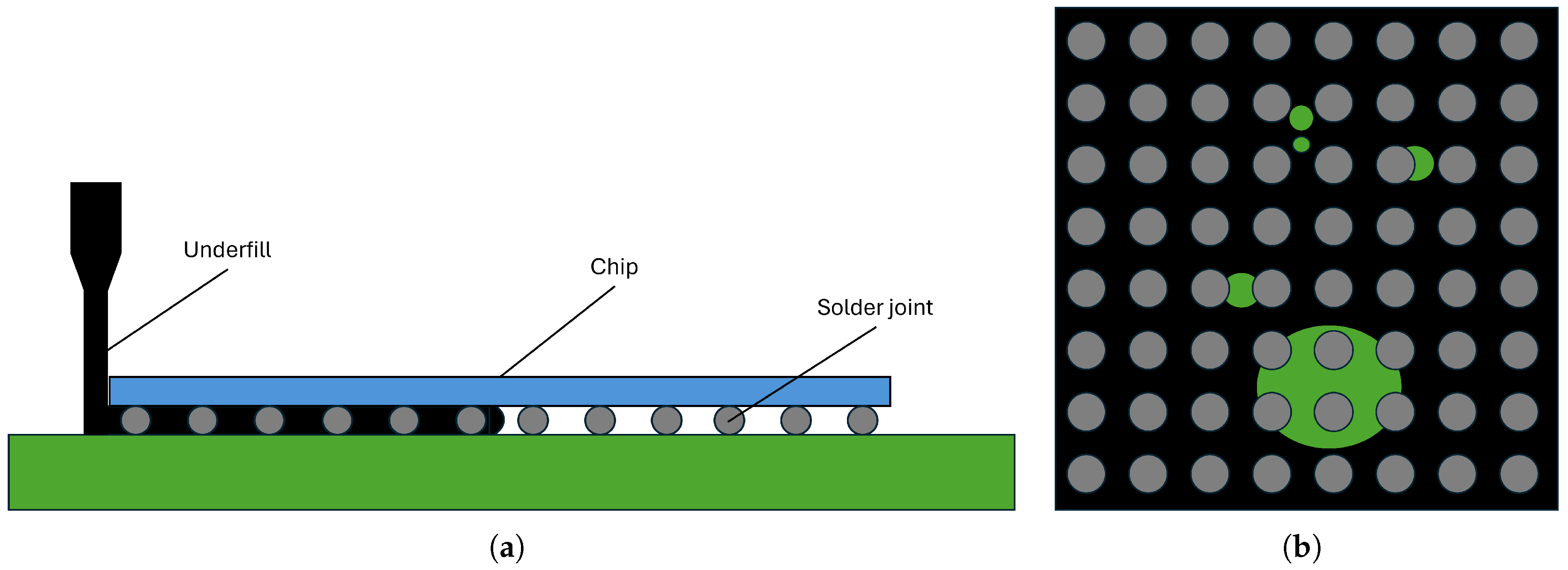
The Material Point Method has certain advantages over other meshless methods, and significant improvements have been made to its stability, efficiency, and accuracy. It can simulate fluids, flow fronts, contacts, multiphysics, and dynamic loading. This gives the impression that MPM is a mature method with few changes happening to it. However, the development of MPM is continuing and is a frequent subject of research. To illustrate the continuing need for MPM improvements, we present a step-by-step simulation of the capillary underfill process that highlights the method’s challenges. Underfill is used to protect the connection between a semiconductor device and the printed circuit board. The underfill process starts with a chip mounted to the substrate with solder joints. The underfill is dispensed along the sides of the chip, where it flows underneath the chip through capillary action, as illustrated in Figure 3a. For a successful filling, the underfill needs to navigate around all the solder joints and completely fill the gap between chip and substrate without leaving any voids. An example of an unsuccessful underfill is shown in Figure 3b. Once filled, it is placed in an oven where the underfill material solidifies, a process known as curing [154].

A simulation of this process must be able to predict: (1) how long it takes to fill the gap between chip and substrate, (2) if voids occur during the process, including their position size and shape, (3) the residual stress left behind on the solder joint and substrate after curing, and (4) the fracturing of the underfill during the lifetime of the microelectronic device. It must also be able to simulate this with reasonable efficiency. A mesh-based simulation of a simplified package was conducted in [155], but it requires extensive remeshing and is not always accurate. To the best of the authors’ knowledge, a fully coupled MPM simulation of the complete underfill process has not yet been reported in the literature. The following discussion therefore evaluates MPM capabilities in terms of the individual physical phenomena required for underfill prediction and assesses which components have been demonstrated and which remain open research challenges. An MPM simulation can improve the flow results because, as already discussed previously, it can simulate fluids and the free surfaces, as well as the contact between underfill and solder joints. It can do this without the need for remeshing. The capillary flow is driven by a pressure gradient between flow front and inlet given by the equation [155]

$$\Delta p={\displaystyle \frac{2\sigma cos\theta }{h}},$$

(23)

where $\sigma$ is the surface tension, $\theta$ the contact angle, and h the distance between chip and substrate. Accurate prediction of the surface tension $\sigma$ requires accurate stress, and thus pressure, results throughout the simulation. Implementing stabilization techniques, such as VMS [98], can greatly reduce the spurious pressure oscillations. It should be noted that (23) assumes steady-state capillary equilibrium with constant surface tension and a static contact angle. Extensions of MPM toward more advanced wetting descriptions have been reported in the literature. For example, contact angle specification through surface tension ratios has been implemented in [156], while surface tension values consistent with prescribed contact angles have been explored in [157]. Furthermore, non-Newtonian flow has been modeled with MPM (e.g., [158]). Fully coupled thermo-capillary effects, including temperature dependent surface tension and dynamic contact angle hysteresis, would require additional thermomechanical coupling and dynamic wetting models. While feasible within the MPM framework, such extensions increase model complexity and are beyond the scope of the present review.

Stabilized MPM might be sufficient to predict filling times, but that still leaves the question of void predictions. The literature shows voids in the underfill most commonly form due to merging flow fronts. The underfill flows around the solder joints and merges behind it, so that is where most voids are found. From a numerical perspective, this requires a finer discretization close to the solder joints and coarser resolution further away to reduce computational cost, so increasing the adaptivity of MPM is desired here. Truncated Hierarchical B-splines [159] (THB) can be a solution here. Hierarchical splines allow the background grid to be refined locally. Truncation maintains partition of unity, ensuring that conservation properties are preserved across refinement levels. In typical implementations, hierarchical refinement is performed dyadically, such that each refinement level reduces the element size by a factor of two relative to the coarser grid. This enables local resolution enhancement where the merging flow fronts and void formation occurs without refining the entire computational domain. Consequently, THB refinement can reduce the overall computational cost compared to a uniformly fine discretization while still resolving the characteristic void length scales. While MPM has demonstrated free surface tracking, predictive void formation in realistic underfill geometries remains an open research problem. Once the filling time and void formation have been predicted, the underfill is cured. Heat is applied solidifying the underfill, which shrinks during the process. Any MPM simulation of the curing needs to include this phase change. Within MPM, the phase change can be incorporated by assigning temperature-dependent constitutive behavior to material points, allowing viscosity, stiffness, and density to evolve with temperature. In [66], the material properties in a given cell are determined by $\psi =\alpha {\psi }_{solid}+(1-\alpha ){\psi }_{liquid}$, where $\psi$ is any material property and $\alpha$ the volumetric fraction. Intermittent stages can be included as well, for example, the glass transition phase. However, the underfill does not shrink uniformly, or more accurately, the temperature increases first at the outer edges and then conducts inwards. Part of the underfill solidifies and shrinks, moving the still liquid underfill into the created space. It is important to include this effect because it will have a significant effect on the eventual size and shape of the voids and the resulting stresses. Simulating this requires solving thermal–fluid–structure interactions with phase changes. This introduces additional numerical challenges, particularly near the moving solidification front, where strong contrasts between liquid and solid behavior can lead to increased time step sensitivity. The critical time step for solid mechanics problems is much smaller than for fluid and heat transfer problems. Hybrid MPM-FEM formulations could be advantageous in this context, using MPM for the liquid underfill and FEM for lightly deforming regions such as the already solidified underfill. This can reduce computational cost while leveraging the strengths of both methods [102]. MPM has shown promise in solving similar multiphysics problems in additive manufacturing [66], suggesting feasibility for underfill curing.

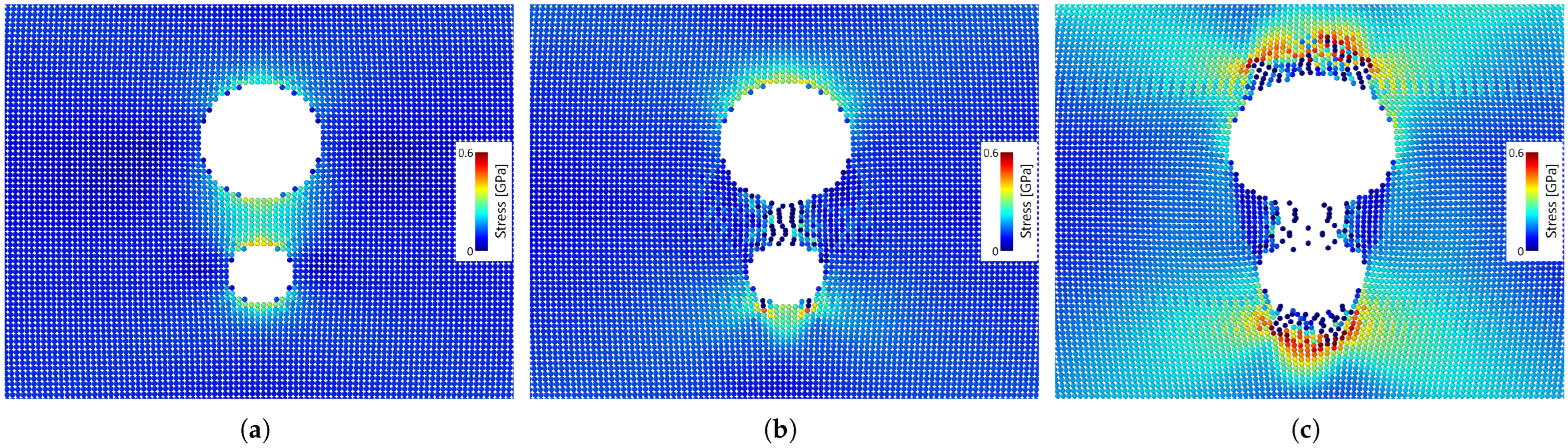
MPM is a good candidate for the prediction of crack propagation in the underfill. It has been used extensively for fracture simulations in a variety of problems. Recently a study was made on crack propagation in the underfill using MPM. Underfills with voids of different sizes and relative distances were modeled using a Johnson–Cook damage model [160]. Figure 4 clearly shows the stress concentrations due to the presence of the voids. These concentrations shift when a crack appears, which causes the crack to propagate further into the underfill, eventually leading to the failure of the device.

Simulating the underfill process with MPM involves multiple length scales, from the mm-scale package and solder joints down to micron-scale voids. Capturing fine features such as voids behind solder joints therefore requires high spatial resolution locally, which can dramatically increase memory and processing requirements. Adaptive or hierarchical grid strategies, such as THB splines, allow refinement only in regions of interest, reducing the total point count while maintaining accuracy in critical areas. Despite these strategies, fully resolving all relevant scales in a realistic package remains computationally challenging, and multiscale MPM simulations of industrial underfill processes are currently in development.

5. Conclusions

This review assessed the suitability of MPM for addressing the simulation challenges in the microelectronics industry, beginning with an overview of the strengths and weaknesses of prominent meshless methods. SPH, EFG, peridynamics, RBF-FD, and MPM were compared in five areas: (1) convergence, consistency, and stability, (2) boundary enforcement, (3) adaptivity, (4) coupling, and (5) industrial applicability.

Regarding convergence, consistency, and stability, all reviewed methods demonstrate reliable performance in specific applications, though formal analysis remains challenging due to moving integration points or nonlocal formulations. Stabilization strategies have been developed across methods, with recent MPM variants (e.g., BSMPM, CPDI, TLMPM) significantly improving robustness. For boundary enforcement, purely particle-based methods such as SPH and peridynamics face greater challenges due to the absence of fixed boundary nodes, often requiring additional techniques. Methods with background grids, such as EFG and MPM, benefit from structured integration frameworks, although boundary treatment remains more involved than in classical FEM.

In terms of adaptivity, meshless discretizations naturally allow nonuniform node or particle distributions. However, practical implementation varies: SPH and peridynamics require additional refinement strategies, while grid-based approaches such as MPM can leverage established adaptive mesh refinement techniques. With respect to coupling, all methods have demonstrated hybrid formulations, most commonly with FEM. MPM has been coupled to a comparatively wide range of numerical schemes, reflecting its flexibility in multiphysics settings. Concerning industrial applicability, all meshless methods face barriers to widespread adoption due to the dominance of established mesh-based tools. While implementations exist in research and selected commercial environments, broader industrial integration requires continued improvements in computational efficiency, robustness, benchmarking, and validation.

The second part of the review examined MPM variants, including BSMPM, GIMP, CPDI, and TLMPM, which were developed to mitigate spurious oscillations and improve consistency and stability. These advancements have enabled MPM to address increasingly complex multiphysics problems involving large deformations, evolving interfaces, and phase changes. The underfill process was used as a representative microelectronics use case to illustrate how MPM’s characteristics align with simulation challenges, such as free surface flow, void formation, thermomechanical coupling during curing, and residual stress development. While these capabilities suggest that MPM is a promising framework for such applications, full scale simulations remain computationally demanding. In particular, rigorous benchmarking against established mesh-based approaches and experimental validation for microelectronics applications are still limited in the literature.

Overall, MPM offers a framework capable of handling large deformations, moving interfaces, history-dependent material behavior, and multiphysics coupling within a single formulation. Continued development in theoretical analysis, adaptive refinement, and large-scale computational efficiency will be essential to transition MPM from promising research methodology to a widely adopted industrial tool in microelectronics reliability analysis.

References

1. Umunnakwe, C.; Zawra, I.; Niessner, M.; Rudnyi, E.; Hohlfeld, D.; Bechtold, T. Compact modelling of a thermo-mechanical finite element model of a microelectronic package. Microelectron. Reliab. 2023, 151, 115238. [Google Scholar] [CrossRef]
2. Ng, F.; Abas, A.; Abdullah, M. Finite volume method study on contact line jump phenomena and dynamic contact angle of underfill flow in flip-chip of various bump pitches. IOP Conf. Ser. Mater. Sci. Eng. 2019, 530, 012012. [Google Scholar] [CrossRef]
3. Hafeez, M.B.; Krawczuk, M. A Review: Applications of the Spectral Finite Element Method. Arch. Comput. Methods Eng. 2023, 30, 3453–3465. [Google Scholar] [CrossRef]
4. Oliveira, S.P.; Seriani, G. Effect of Element Distortion on the Numerical Dispersion of Spectral Element Methods. Commun. Comput. Phys. 2011, 9, 937–958. [Google Scholar] [CrossRef]
5. Weiss, M.; Kalscheuer, T.; Ren, Z. Spectral element method for 3-D controlled-source electromagnetic forward modelling using unstructured hexahedral meshes. Geophys. J. Int. 2022, 232, 1427–1454. [Google Scholar] [CrossRef]
6. Feng, Y.; Wu, D.; Stewart, M.G.; Gao, W. Past, current and future trends and challenges in non-deterministic fracture mechanics: A review. Comput. Methods Appl. Mech. Eng. 2023, 412, 116102. [Google Scholar] [CrossRef]
7. Cervera, M.; Barbat, G.B.; Chiumenti, M.; Wu, J.Y. A Comparative Review of XFEM, Mixed FEM and Phase-Field Models for Quasi-brittle Cracking. Arch. Comput. Methods Eng. 2022, 29, 1009–1083. [Google Scholar] [CrossRef]
8. Vellwock, A.E.; Libonati, F. XFEM for Composites, Biological, and Bioinspired Materials: A Review. Materials 2024, 17, 745. [Google Scholar] [CrossRef] [PubMed]
9. Spühler, J.H.; Jansson, J.; Jansson, N.; Hoffman, J. 3D fluid-structure interaction simulation of aortic valves using a unified continuum ALE FEM model. Front. Physiol. 2018, 9, 363. [Google Scholar] [CrossRef]
10. Gao, P.; Hu, X. The development of an ALE finite element and discontinuous Galerkin method for the non-isothermal non-Newtonian FSI problem. Eng. Comput. 2025, 41, 99–116. [Google Scholar] [CrossRef]
11. Liu, S.; Tang, X.; Li, J. Extension of ALE method in large deformation analysis of saturated soil under earthquake loading. Comput. Geotech. 2021, 133, 104056. [Google Scholar] [CrossRef]
12. Baiges, J.; Codina, R.; Pont, A.; Castillo, E. An adaptive Fixed-Mesh ALE method for free surface flows. Comput. Methods Appl. Mech. Eng. 2017, 313, 159–188. [Google Scholar] [CrossRef]
13. Zhang, W.; Zhang, X.; He, L.; Li, P. The damage characteristics and formation mechanism of ultrahigh strength 7055 aluminum alloy under hypervelocity impact. Int. J. Impact Eng. 2023, 180, 104718. [Google Scholar] [CrossRef]
14. Wang, Y.; Mao, Z.; Yu, C.; Li, X.; Wang, X.; Yan, H. Numerical simulation of hypervelocity impact of the water-filled aluminum eggshell array structure using material point method. Phys. Fluids 2025, 37, 037104. [Google Scholar] [CrossRef]
15. Morikawa, D.S.; Tsuji, K.; Asai, M. Corrected ALE-ISPH with novel Neumann boundary condition and density-based particle shifting technique. J. Comput. Phys. X 2023, 17, 100125. [Google Scholar] [CrossRef]
16. Zhang, F.; Zhang, X.; Sze, K.Y.; Liang, Y.; Liu, Y. Improved incompressible material point method based on particle density correction. Int. J. Comput. Methods 2018, 15, 1850061. [Google Scholar] [CrossRef]
17. Baumgarten, A.S.; Kamrin, K. Analysis and mitigation of spatial integration errors for the material point method. Int. J. Numer. Methods Eng. 2023, 124, 2449–2497. [Google Scholar] [CrossRef]
18. de Vaucorbeil, A.; Phu Nguyen, V.; Sinaie, S.; Wu, J.Y. Material point method after 25 years: Theory, implementation and applications. Adv. Appl. Mech. 2020, 53, 185–398. [Google Scholar] [CrossRef]
19. Nguyen, V.P.; De Vaucorbeil, A.; Bordas, S. The Material Point Method Theory, Implementations and Applications; Springer: Durham, NC, USA, 2023. [Google Scholar] [CrossRef]
20. Vacondio, R.; Altomare, C.; De Leffe, M.; Hu, X.; Le Touzé, D.; Lind, S.; Marongiu, J.C.; Marrone, S.; Rogers, B.D.; Souto-Iglesias, A. Grand challenges for Smoothed Particle Hydrodynamics numerical schemes. Comput. Part. Mech. 2020, 8, 575–588. [Google Scholar] [CrossRef]
21. Gingold, R.A.; Monaghan, J.J. Smoothed particle hydrodynamics: Theory and application to non-spherical stars. Mon. Not. R. Astron. Soc. 1977, 181, 375–389. [Google Scholar] [CrossRef]
22. Sun, P.N.; Colagrossi, A.; Marrone, S.; Antuono, M.; Zhang, A.M. Multi-resolution Delta-plus-SPH with tensile instability control: Towards high Reynolds number flows. Comput. Phys. Commun. 2018, 224, 63–80. [Google Scholar] [CrossRef]
23. Zhang, Y.; Yang, D.; Jin, X.; Zheng, Y.; Fu, H.; Ji, J.; Yang, Z. Multiscale friction-impact dynamics in piezoelectric motors via SPH/FEM. Int. J. Mech. Sci. 2026, 311, 111182. [Google Scholar] [CrossRef]
24. Qian, Y.; Usher, S.P.; Scales, P.J.; Stickland, A.D.; Alexiadis, A. Agglomeration Regimes of Particles under a Linear Laminar Flow: A Numerical Study. Mathematics 2022, 10, 1931. [Google Scholar] [CrossRef]
25. Belytschko, T.; Lu, Y.Y.; Gu, L. Element-free Galerkin methods. Int. J. Numer. Methods Eng. 1994, 37, 229–256. [Google Scholar] [CrossRef]
26. Lancaster, P.; Salkauskas, K. Surfaces generated by moving least squares methods. Math. Comput. 1981, 37, 141–158. [Google Scholar] [CrossRef]
27. Tey, W.Y.; Asako, Y.; Ng, K.C.; Lam, W.H. A review on development and applications of element-free galerkin methods in computational fluid dynamics. Int. J. Comput. Methods Eng. Sci. Mech. 2020, 21, 252–275. [Google Scholar] [CrossRef]
28. Zhang, T.; Li, X. Analysis of the Element-Free Galerkin Method with Penalty for Stokes Problems. Entropy 2022, 24, 1072. [Google Scholar] [CrossRef] [PubMed]
29. Ma, H.; Chen, J.; Deng, J. Analysis of the dynamic response for Kirchhoff plates by the element-free Galerkin method. J. Comput. Appl. Math. 2024, 451, 116093. [Google Scholar] [CrossRef]
30. Akhil, S.L.; Krishna, I.R.; Aswathy, M. Effect of non-dimensional length scale in element free Galerkin method for classical and strain driven nonlocal elasto-static problems. Comput. Struct. 2025, 312, 107724. [Google Scholar] [CrossRef]
31. Akhil, S.L.; Krishna, I.R.P. Element-Free Galerkin Method for Elastostatic Analysis of Nonlocal Stress-Driven Bernoulli–Euler Beams. J. Eng. Mech. 2025, 151, 04025050. [Google Scholar] [CrossRef]
32. Häussler-Combe, U.; Korn, C. An adaptive approach with the Element-Free-Galerkin method. Comput. Methods Appl. Mech. Eng. 1998, 162, 203–222. [Google Scholar] [CrossRef]
33. Le, C.V.; Askes, H.; Gilbert, M. Adaptive element-free Galerkin method applied to the limit analysis of plates. Comput. Methods Appl. Mech. Eng. 2010, 199, 2487–2496. [Google Scholar] [CrossRef]
34. Zhang, X.; Zhang, P.; Qin, W.; Shi, X. An adaptive variational multiscale element free Galerkin method for convection–diffusion equations. Eng. Comput. 2022, 38, 3373–3390. [Google Scholar] [CrossRef]
35. Liu, F.; Zuo, M.; Cheng, H.; Ma, J. Analyzing Three-Dimensional Laplace Equations Using the Dimension Coupling Method. Mathematics 2023, 11, 3717. [Google Scholar] [CrossRef]
36. Álvarez-Hostos, J.C.; Ullah, Z.; Storti, B.A.; Tourn, B.A.; Zambrano-Carrillo, J.A. An overset improved element-free Galerkin-finite element method for the solution of transient heat conduction problems with concentrated moving heat sources. Comput. Methods Appl. Mech. Eng. 2024, 418, 116574. [Google Scholar] [CrossRef]
37. Zambrano-Carrillo, J.A.; Álvarez-Hostos, J.C.; Serebrinsky, S.; Huespe, A.E. Solving linear elasticity benchmark problems via the overset improved element-free Galerkin-finite element method. Finite Elem. Anal. Des. 2024, 241, 104247. [Google Scholar] [CrossRef]
38. Wang, S.; Qian, H.; Ju, L. Topology optimization for minimizing the mean compliance under thermo-mechanical loads using element-free Galerkin method. Appl. Math. Model. 2024, 136, 115630. [Google Scholar] [CrossRef]
39. Zhou, L.; Wang, J.; Li, X.; Liu, C.; Liu, P.; Ren, S.; Li, M. The magneto-electro-elastic multi-physics coupling element free Galerkin method for smart structures in statics and dynamics problems. Thin-Walled Struct. 2021, 169, 108431. [Google Scholar] [CrossRef]
40. Foss, M.; Radu, P.; Yu, Y. Convergence Analysis and Numerical Studies for Linearly Elastic Peridynamics with Dirichlet-Type Boundary Conditions. J. Peridyn. Nonlocal Model. 2023, 5, 275–310. [Google Scholar] [CrossRef]
41. Jin, S.; Hong, J.W. Convergence study of stabilized non-ordinary state-based peridynamics for elastic and fracture problems. Eng. Fract. Mech. 2023, 289, 109438. [Google Scholar] [CrossRef]
42. Madenci, E.; Oterkus, E. Peridynamic Theory and Its Applications; Springer: New York, NY, USA, 2014; pp. 1–289. ISBN 9781461484653. [Google Scholar] [CrossRef]
43. Ren, H.; Zhuang, X.; Cai, Y.; Rabczuk, T. Dual-horizon peridynamics. Int. J. Numer. Methods Eng. 2016, 108, 1451–1476. [Google Scholar] [CrossRef]
44. Ou, X.; Yao, X.; Han, F. An adaptive coupling modeling between peridynamics and classical continuum mechanics for dynamic crack propagation and crack branching. Eng. Fract. Mech. 2023, 281, 109096. [Google Scholar] [CrossRef]
45. Sun, W.; Fish, J.; Lin, P. Numerical simulation of fluid-driven fracturing in orthotropic poroelastic media based on a peridynamics-finite element coupling approach. Int. J. Rock Mech. Min. Sci. 2022, 158, 105199. [Google Scholar] [CrossRef]
46. Dai, Z.; Xie, J.; Jiang, M. A coupled peridynamics–smoothed particle hydrodynamics model for fracture analysis of fluid–structure interactions. Ocean Eng. 2023, 279, 114582. [Google Scholar] [CrossRef]
47. Gonda, G.; Gábor Ladányi, V.; Gonda, V. Review of Peridynamics: Theory, Applications, and Future Perspectives. Stroj. Vestn.-J. Mech. Eng. 2021, 67, 666–681. [Google Scholar] [CrossRef]
48. Bayona, V.; Moscoso, M.; Carretero, M.; Kindelan, M. RBF-FD formulas and convergence properties. J. Comput. Phys. 2010, 229, 8281–8295. [Google Scholar] [CrossRef]
49. Flyer, N.; Lehto, E.; Blaise, S.; Wright, G.B.; St-Cyr, A. A guide to RBF-generated finite differences for nonlinear transport: Shallow water simulations on a sphere. J. Comput. Phys. 2012, 231, 4078–4095. [Google Scholar] [CrossRef]
50. Mishra, P.K.; Fasshauer, G.E.; Sen, M.K.; Ling, L. A stabilized radial basis-finite difference (RBF-FD) method with hybrid kernels. Comput. Math. Appl. 2019, 77, 2354–2368. [Google Scholar] [CrossRef]
51. Jančič, M.; Slak, J.; Kosec, G. Monomial augmentation guidelines for RBF-FD from accuracy versus computational time perspective. J. Sci. Comput. 2021, 87, 9. [Google Scholar] [CrossRef]
52. Li, J.; Zhai, S.; Weng, Z.; Feng, X. H-adaptive RBF-FD method for the high-dimensional convection-diffusion equation. Int. Commun. Heat Mass Transf. 2017, 89, 139–146. [Google Scholar] [CrossRef]
53. Cao, J.; Liu, Y.; Yin, C.; Wang, H.; Su, Y.; Wang, L.; Ma, X.; Zhang, B. Hybrid meshless-FEM method for 3-D magnetotelluric modelling using non-conformal discretization. Geophys. J. Int. 2024, 238, 1181–1200. [Google Scholar] [CrossRef]
54. Vuga, G.; Mavrič, B.; Šarler, B. A hybrid radial basis function-finite difference method for modelling two-dimensional thermo-elasto-plasticity, Part 1: Method formulation and testing. Eng. Anal. Bound. Elem. 2024, 159, 58–67. [Google Scholar] [CrossRef]
55. Vuga, G.; Mavrič, B.; Dobravec, T.; Šarler, B. A hybrid radial basis function-finite difference method for modelling two-dimensional thermo-elasto-plasticity, Part 3: Application to thermo-mechanical modelling of continuous casting of steel billets. Eng. Anal. Bound. Elem. 2026, 183, 106619. [Google Scholar] [CrossRef]
56. Fornberg, B.; Flyer, N. A Primer on Radial Basis Functions with Applications to the Geosciences; SIAM: Philadelphia, PA, USA, 2015. [Google Scholar] [CrossRef]
57. Milovanović, S.; Von Sydow, L. Radial basis function generated finite differences for option pricing problems. Comput. Math. Appl. 2018, 75, 1462–1481. [Google Scholar] [CrossRef]
58. Telikicherla, R.M.; Moutsanidis, G. An assessment of the total Lagrangian material point method: Comparison to conventional MPM, higher order basis, and treatment of near-incompressibility. Comput. Methods Appl. Mech. Eng. 2023, 414, 116135. [Google Scholar] [CrossRef]
59. Hu, P.; Xue, L.; Qu, K.; Ni, K.; Brenner, M.J. Unified solver for modeling and simulation of nonlinear aeroelasticity and fluid-structure interactions. In AIAA Atmospheric Flight Mechanics Conference; American Institute of Aeronautics and Astronautics Inc.: Reston, VA, USA, 2009. [Google Scholar] [CrossRef]
60. Hu, P.G.; Xue, L.; Mao, S.; Kamakoti, R.; Zhao, H.; Dittakavi, N.; Ni, K.; Wang, Z.; Li, Q. Material point method applied to fluid-structure interaction (FSI)/aeroelasticity problems. In 48th AIAA Aerospace Sciences Meeting Including the New Horizons Forum and Aerospace Exposition; American Institute of Aeronautics and Astronautics Inc.: Reston, VA, USA, 2010. [Google Scholar] [CrossRef]
61. Zhang, K.; Shen, S.L.; Zhou, A.; Balzani, D. Truncated hierarchical B-spline material point method for large deformation geotechnical problems. Comput. Geotech. 2021, 134, 104097. [Google Scholar] [CrossRef]
62. Feng, K.; Huang, D.; Wang, G.; Jin, F.; Chen, Z. Physics-based large-deformation analysis of coseismic landslides: A multiscale 3D SEM-MPM framework with application to the Hongshiyan landslide. Eng. Geol. 2022, 297, 106487. [Google Scholar] [CrossRef]
63. Raymond, S.J.; Jones, B.; Williams, J.R. A strategy to couple the material point method (MPM) and smoothed particle hydrodynamics (SPH) computational techniques. Comput. Part. Mech. 2018, 5, 49–58. [Google Scholar] [CrossRef]
64. Jiang, C.; Schroeder, C.; Teran, J.; Stomakhin, A.; Selle, A. The material point method for simulating continuum materials. In ACM SIGGRAPH 2016 Courses, SIGGRAPH 2016; Association for Computing Machinery: New York, NY, USA, 2016. [Google Scholar] [CrossRef]
65. Stomakhin, A.; Schroeder, C.; Chai, L.; Teran, J.; Selle, A. A material point method for snow simulation. ACM Trans. Graph. 2013, 32, 1–10. [Google Scholar] [CrossRef]
66. Lian, Y.; Chen, J.; Li, M.J.; Gao, R. A multi-physics material point method for thermo-fluid-solid coupling problems in metal additive manufacturing processes. Comput. Methods Appl. Mech. Eng. 2023, 416, 116297. [Google Scholar] [CrossRef]
67. Song, X.; Yang, Y.; Cheng, Y.; Wang, Y.; Zheng, H. Study on copper-stainless steel explosive welding for nuclear fusion by generalized interpolated material point method and experiments. Eng. Anal. Bound. Elem. 2024, 160, 160–172. [Google Scholar] [CrossRef]
68. Zhang, Y.; Zhu, S.; Zhao, Y.; Yin, Y. A material point method based investigation on crack classification and transformation induced by grit geometry during scratching silicon carbide. Int. J. Mach. Tools Manuf. 2022, 177, 103884. [Google Scholar] [CrossRef]
69. Leroch, S.; Eder, S.J.; Ganzenmüller, G.; Murillo, L.J.; Rodríguez Ripoll, M. Development and validation of a meshless 3D material point method for simulating the micro-milling process. J. Mater. Process. Technol. 2018, 262, 449–458. [Google Scholar] [CrossRef]
70. Ambati, R.; Pan, X.; Yuan, H.; Zhang, X. Application of material point methods for cutting process simulations. Comput. Mater. Sci. 2012, 57, 102–110. [Google Scholar] [CrossRef]
71. Saffarini, M.H.; Chen, Z.; Elbelbisi, A.; Salim, H.; Perry, K.; Bowman, A.L.; Robert, S.D. Verification and Validation of Modeling of Fluid–Solid Interaction in Explosion-Resistant Designs Using Material Point Method. Buildings 2024, 14, 3137. [Google Scholar] [CrossRef]
72. Povolny, S.J.; Homel, M.A.; Herbold, E.B. Assessing and improving strong-shock accuracy in the material point method. Comput. Methods Appl. Mech. Eng. 2023, 416, 116350. [Google Scholar] [CrossRef]
73. Ikkurthi, V.R.; Rahulnath, P.P.; Mehra, V.; Warrier, M.; Dasgupta, K.; Savita, A.N.; Pahari, S.; Alexander, R.; Arya, A.; Malshe, U.D. Computational and experimental studies of penetration resistance of Ceramic-Metal composites. Mater. Today Proc. 2023, 87, 257–262. [Google Scholar] [CrossRef]
74. Li, M.; Lei, Y.; Gao, D.; Hu, Y.; Zhang, X. A novel material point method (MPM) based needle-tissue interaction model. Comput. Methods Biomech. Biomed. Eng. 2021, 24, 1393–1407. [Google Scholar] [CrossRef] [PubMed]
75. Sung, S.K.; Kim, J.H.; Shin, B.S. Material Point Method-Based Simulation Techniques for Medical Applications. Electronics 2024, 13, 1340. [Google Scholar] [CrossRef]
76. Nazemi, A.; Milani, A.S. A comparative study of emerging material point method and FEM for forming simulation of textile reinforcements. Compos. Part A Appl. Sci. Manuf. 2024, 185, 108284. [Google Scholar] [CrossRef]
77. Xu, J.; Chen, X.; Zhong, W.; Wang, F.; Zhang, X. An improved material point method for coining simulation. Int. J. Mech. Sci. 2021, 196, 106258. [Google Scholar] [CrossRef]
78. Yin, Y.; Xu, J.; Dong, J.; Li, Y.; Wang, Y.; Zhong, W.; Zhang, Z. Cuda-based parallel dual-grid material point method for simulating bimetallic coining process. Comput. Part. Mech. 2025, 12, 4653–4676. [Google Scholar] [CrossRef]
79. Davy, J.; Lloyd, P.; Chandler, J.H.; Valdastri, P. A Framework for Simulation of Magnetic Soft Robots Using the Material Point Method. IEEE Robot. Autom. Lett. 2023, 8, 3470–3477. [Google Scholar] [CrossRef]
80. Maeshima, T.; Kim, Y.; Zohdi, T.I. Particle-scale numerical modeling of thermo-mechanical phenomena for additive manufacturing using the material point method. Comput. Part. Mech. 2021, 8, 613–623. [Google Scholar] [CrossRef]
81. Germain, J.D.d.S.; McCorquodale, J.; Parker, S.G.; Johnson, C.R. Uintah: A massively parallel problem solving environment. In Ninth International Symposium on High-Performance Distributed Computing; IEEE: Piscataway, NJ, USA, 2000; pp. 33–41. [Google Scholar] [CrossRef]
82. de Vaucorbeil, A.; Nguyen, V.P.; Nguyen-Thanh, C. Karamelo: An open source parallel C++ package for the material point method. Comput. Part. Mech. 2021, 8, 767–789. [Google Scholar] [CrossRef]
83. Kumar, K.; Salmond, J.; Kularathna, S.; Wilkes, C.; Tjung, E.; Biscontin, G.; Soga, K. Scalable and modular material point method for large-scale simulations. arXiv 2019, arXiv:1909.13380. [Google Scholar] [CrossRef]
84. Hu, Y.; Fang, Y.; Ge, Z.; Qu, Z.; Zhu, Y.; Pradhana, A.; Jiang, C. A Moving Least Squares Material Point Method with Displacement Discontinuity and Two-Way Rigid Body Coupling. ACM Trans. Graph. (TOG) 2018, 37, 150. [Google Scholar] [CrossRef]
85. Zhu, Z.; Bao, T.; Zhu, X.; Gong, J.; Hu, Y.; Zhang, J. An Improved Material Point Method with Aggregated and Smoothed Bernstein Functions. Mathematics 2023, 11, 907. [Google Scholar] [CrossRef]
86. Steffen, M.; Kirby, R.M.; Berzins, M. Analysis and reduction of quadrature errors in the material point method (MPM). Int. J. Numer. Meth. Eng. 2008, 76, 922–948. [Google Scholar] [CrossRef]
87. Gan, Y.; Sun, Z.; Chen, Z.; Zhang, X.; Liu, Y. Enhancement of the material point method using B-spline basis functions. Int. J. Numer. Methods Eng. 2018, 113, 411–431. [Google Scholar] [CrossRef]
88. Nakamura, K.; Matsumura, S.; Mizutani, T. Particle-to-surface frictional contact algorithm for material point method using weighted least squares. Comput. Geotech. 2021, 134, 104069. [Google Scholar] [CrossRef]
89. Sang, Q.; Xiong, Y.; Zheng, R.; Bao, X.; Ye, G.; Zhang, F. A hybrid contact approach for modeling soil-structure interaction using the material point method. J. Rock Mech. Geotech. Eng. 2024, 16, 1864–1882. [Google Scholar] [CrossRef]
90. Bardenhagen, S.G.; Kober, E.M. The Generalized Interpolation Material Point Method. Comput. Model. Eng. Sci. 2004, 5, 477–495. [Google Scholar] [CrossRef]
91. Sadeghirad, A.; Brannon, R.M.; Burghardt, J. A convected particle domain interpolation technique to extend applicability of the material point method for problems involving massive deformations. Int. J. Numer. Methods Eng. 2011, 86, 1435–1456. [Google Scholar] [CrossRef]
92. Sadeghirad, A.; Brannon, R.M.; Guilkey, J.E. Second-order convected particle domain interpolation (CPDI2) with enrichment for weak discontinuities at material interfaces. Int. J. Numer. Methods Eng. 2013, 95, 928–952. [Google Scholar] [CrossRef]
93. Sadeghirad, A. B-spline convected particle domain interpolation method. Eng. Anal. Bound. Elem. 2024, 160, 106–133. [Google Scholar] [CrossRef]
94. Homel, M.A.; Brannon, R.M.; Guilkey, J. Controlling the onset of numerical fracture in parallelized implementations of the material point method (MPM) with convective particle domain interpolation (CPDI) domain scaling. Int. J. Numer. Methods Eng. 2016, 107, 31–48. [Google Scholar] [CrossRef]
95. Renaud, A.; Heuzé, T. A discontinuous galerkin material point method (DGMPM) for the simulation of impact problems in solid mechanics. In COMPDYN 2017—Proceedings of the 6th International Conference on Computational Methods in Structural Dynamics and Earthquake Engineering; National Technical University of Athens: Zografou, Greece, 2017; Volume 2, pp. 3728–3738. [Google Scholar] [CrossRef]
96. de Vaucorbeil, A.; Nguyen, V.P.; Hutchinson, C.R. A Total-Lagrangian Material Point Method for solid mechanics problems involving large deformations. Comput. Methods Appl. Mech. Eng. 2020, 360, 112783. [Google Scholar] [CrossRef]
97. de Vaucorbeil, A.; Nguyen, V.P. Modelling contacts with a total Lagrangian material point method. Comput. Methods Appl. Mech. Eng. 2021, 373, 113503. [Google Scholar] [CrossRef]
98. Chandra, B.; Hashimoto, R.; Matsumi, S.; Kamrin, K.; Soga, K. Stabilized mixed material point method for incompressible fluid flow analysis. Comput. Methods Appl. Mech. Eng. 2024, 419, 116644. [Google Scholar] [CrossRef]
99. Kularathna, S.; Liang, W.; Zhao, T.; Chandra, B.; Zhao, J.; Soga, K. A semi-implicit material point method based on fractional-step method for saturated soil. Int. J. Numer. Anal. Methods Geomech. 2021, 45, 1405–1436. [Google Scholar] [CrossRef]
100. Molinos, M.; Chandra, B.; Stickle, M.M.; Soga, K. On the derivation of a component-free scheme for Lagrangian fluid–structure interaction problems. Acta Mech. 2023, 234, 1777–1809. [Google Scholar] [CrossRef]
101. Li, M.J.; Lian, Y.; Zhang, X. An immersed finite element material point (IFEMP) method for free surface fluid–structure interaction problems. Comput. Methods Appl. Mech. Eng. 2022, 393, 114809. [Google Scholar] [CrossRef]
102. Li, M.J.; Lian, Y.; Liu, X.; Chen, J.; Lei, L.; Shi, L. Adaptive multi-physics finite element-material point method with two-way conversion between elements and particles for metal additive manufacturing. Comput. Methods Appl. Mech. Eng. 2025, 446, 118263. [Google Scholar] [CrossRef]
103. Molinos, M.; Navas, P.; Manzanal, D.; Pastor, M. Local Maximum Entropy Material Point Method applied to quasi-brittle fracture. Eng. Fract. Mech. 2021, 241, 107394. [Google Scholar] [CrossRef]
104. Molinos, M.; Martín Stickle, M.; Navas, P.; Yagüe, Á.; Manzanal, D.; Pastor, M. Toward a local maximum-entropy material point method at finite strain within a B-free approach. Int. J. Numer. Methods Eng. 2021, 122, 5594–5625. [Google Scholar] [CrossRef]
105. Molinos, M.; Navas, P.; Pastor, M.; Stickle, M.M. On the dynamic assessment of the Local-Maximum Entropy Material Point Method through an Explicit Predictor–Corrector Scheme. Comput. Methods Appl. Mech. Eng. 2021, 374, 113512. [Google Scholar] [CrossRef]
106. Qian, Z.; Wang, L.; Zhang, C.; Chen, Q. A highly efficient and accurate Lagrangian–Eulerian stabilized collocation method (LESCM) for the fluid–rigid body interaction problems with free surface flow. Comput. Methods Appl. Mech. Eng. 2022, 398, 115238. [Google Scholar] [CrossRef]
107. Qian, Z.; Wang, L.; Zhang, C.; Zhong, Z.; Chen, Q. Conservation and accuracy studies of the LESCM for incompressible fluids. J. Comput. Phys. 2023, 489, 112269. [Google Scholar] [CrossRef]
108. Qian, Z.; Liu, M.; Wang, L.; Zhang, C. Extraction of Lagrangian Coherent Structures in the framework of the Lagrangian–Eulerian Stabilized Collocation Method (LESCM). Comput. Methods Appl. Mech. Eng. 2023, 416, 116372. [Google Scholar] [CrossRef]
109. Qian, Z.; Liu, M.; Shen, W. A deformation-dependent visualization scheme in the framework of the Material Point Method. Comput. Part. Mech. 2024, 12, 4751–4770. [Google Scholar] [CrossRef]
110. Qian, Z.; Yang, T.; Liu, M. An Overview of Coupled Lagrangian–Eulerian Methods for Ocean Engineering. J. Mar. Sci. Appl. 2024, 23, 366–397. [Google Scholar] [CrossRef]
111. Ren, S.; Zhang, P.; Galindo-Torres, S.A. A coupled discrete element material point method for fluid–solid–particle interactions with large deformations. Comput. Methods Appl. Mech. Eng. 2022, 395, 115023. [Google Scholar] [CrossRef]
112. Ren, S.; Zhang, P.; Zhao, Y.; Tian, X.; Galindo-Torres, S.A. A coupled metaball discrete element material point method for fluid–particle interactions with free surface flows and irregular shape particles. Comput. Methods Appl. Mech. Eng. 2023, 417, 116440. [Google Scholar] [CrossRef]
113. Li, J.; Wang, B.; Wang, D.; Zhang, P.; Vardon, P.J. A coupled MPM-DEM method for modelling soil-rock mixtures. Comput. Geotech. 2023, 160, 105508. [Google Scholar] [CrossRef]
114. Ren, S.; Zhang, P.; Man, T.; Galindo-Torres, S.A. Numerical assessments of the influences of soil–boulder mixed flow impact on downstream facilities. Comput. Geotech. 2023, 153, 105055. [Google Scholar] [CrossRef]
115. Ren, S.; Liu, Z.; Trujillo-Vela, M.G.; Galindo-Torres, S.A.; Tian, X.; Zhang, P. Simulation of solitary wave generation and wave-structure interactions using an MPM-SDEM coupling scheme. Ocean Eng. 2025, 340, 122195. [Google Scholar] [CrossRef]
116. Sang, Q.Y.; Xiong, Y.L.; Zheng, R.Y.; Bao, X.H.; Ye, G.L.; Zhang, F. An implicit coupled MPM formulation for static and dynamic simulation of saturated soils based on a hybrid method. Comput. Mech. 2025, 75, 1033–1060. [Google Scholar] [CrossRef]
117. Sang, Q.y.; Xiong, Y.l.; Zheng, R.y.; Bao, X.h.; Ye, G.l.; Zhang, S. An implicit stabilized material point method for modelling coupled hydromechanical problems in two-phase geomaterials. Comput. Geotech. 2024, 166, 106049. [Google Scholar] [CrossRef]
118. Sang, Q.Y.; Liu, Z.G.; Xiong, Y.L.; Wu, R.X.; Yan, J.H. A Robust Lagrangian Implicit Material Point Method for Accurate Large-Deformation Analysis. Symmetry 2025, 17, 1876. [Google Scholar] [CrossRef]
119. Sun, Z.; Huang, Z.; Zhou, X. Benchmarking the material point method for interaction problems between the free surface flow and elastic structure. Prog. Comput. Fluid Dyn. Int. J. 2019, 19, 1. [Google Scholar] [CrossRef]
120. Sun, Z.; Liu, K.; Wang, J.; Zhou, X. Hydro-mechanical coupled B-spline material point method for large deformation simulation of saturated soils. Eng. Anal. Bound. Elem. 2021, 133, 330–340. [Google Scholar] [CrossRef]
121. Sun, Z.; Gan, Y.; Tao, J.; Huang, Z.; Zhou, X. An improved quadrature scheme in B-spline material point method for large-deformation problem analysis. Eng. Anal. Bound. Elem. 2022, 138, 301–318. [Google Scholar] [CrossRef]
122. Zhou, X.; Hua, Y.; Sun, Z. Application of Cross model for granular flow and impact analysis using three-dimensional B-spline material point method. J. Non-Newton. Fluid Mech. 2023, 322, 105145. [Google Scholar] [CrossRef]
123. Sun, Z.; Hua, Y.; Xu, Y.; Zhou, X. Simulation of fluid-structure interaction using the density smoothing B-spline material point method with a contact approach. Comput. Math. Appl. 2024, 176, 525–544. [Google Scholar] [CrossRef]
124. Moutsanidis, G.; Kamensky, D.; Zhang, D.Z.; Bazilevs, Y.; Long, C.C. Modeling strong discontinuities in the material point method using a single velocity field. Comput. Methods Appl. Mech. Eng. 2019, 345, 584–601. [Google Scholar] [CrossRef]
125. Moutsanidis, G.; Long, C.C.; Bazilevs, Y. IGA-MPM: The Isogeometric Material Point Method. Comput. Methods Appl. Mech. Eng. 2020, 372, 113346. [Google Scholar] [CrossRef]
126. Telikicherla, R.M.; Moutsanidis, G. Treatment of near-incompressibility and volumetric locking in higher order material point methods. Comput. Methods Appl. Mech. Eng. 2022, 395, 114985. [Google Scholar] [CrossRef]
127. Telikicherla, R.M.; Moutsanidis, G. A displacement-based material point method for weakly compressible free-surface flows. Comput. Mech. 2024, 75, 389–405. [Google Scholar] [CrossRef]
128. Tran, Q.A.; Sołowski, W. Temporal and null-space filter for the material point method. Int. J. Numer. Methods Eng. 2019, 120, 328–360. [Google Scholar] [CrossRef]
129. Tran, Q.A.; Grimstad, G.; Ghoreishian Amiri, S.A. MPMICE: A hybrid MPM-CFD model for simulating coupled problems in porous media. Application to earthquake-induced submarine landslides. Int. J. Numer. Methods Eng. 2024, 125, e7383. [Google Scholar] [CrossRef]
130. Tran, Q.A.; Sørlie, E.; Grimstad, G.; Eiksund, G.; Takahashi, H.; Sassa, S. Influence of sediment permeability in seismic-induced submarine landslide mechanism: CFD-MPM validation with centrifuge tests and analysis. Comput. Geotech. 2024, 174, 106588. [Google Scholar] [CrossRef]
131. Sørlie, E.R.; Tran, Q.A.; Eiksund, G.R.; Degago, S.A. Numerical modeling of clay-rich submarine landslides using a novel material point method coupled with computational fluid dynamics. Landslides 2025, 22, 2503–2518. [Google Scholar] [CrossRef]
132. de Vaucorbeil, A.; Nguyen, V.P.; Mandal, T.K. Mesh objective simulations of large strain ductile fracture: A new nonlocal Johnson-Cook damage formulation for the Total Lagrangian Material Point Method. Comput. Methods Appl. Mech. Eng. 2022, 389, 114388. [Google Scholar] [CrossRef]
133. de Vaucorbeil, A.; Nguyen, V.P.; Hutchinson, C.R.; Barnett, M.R. Total Lagrangian Material Point Method simulation of the scratching of high purity coppers. Int. J. Solids Struct. 2022, 239–240, 111432. [Google Scholar] [CrossRef]
134. Buckland, E.; Nguyen, V.P.; de Vaucorbeil, A. Easily porting material point methods codes to GPU. Comput. Part. Mech. 2024, 11, 2127–2142. [Google Scholar] [CrossRef]
135. Bui, Q.H.; Nguyen, V.P.; de Vaucorbeil, A. A New Contact Algorithm for the Total-Lagrangian Material Point Method. Int. J. Numer. Methods Eng. 2025, 126, e70105. [Google Scholar] [CrossRef]
136. Nakamura, K.; Matsumura, S.; Mizutani, T. Taylor particle-in-cell transfer and kernel correction for material point method. Comput. Methods Appl. Mech. Eng. 2023, 403, 115720. [Google Scholar] [CrossRef]
137. Zhao, Y.; Choo, J. Stabilized material point methods for coupled large deformation and fluid flow in porous materials. Comput. Methods Appl. Mech. Eng. 2020, 362, 112742. [Google Scholar] [CrossRef]
138. Zhao, Y.; Jiang, C.; Choo, J. Circumventing volumetric locking in explicit material point methods: A simple, efficient, and general approach. Int. J. Numer. Methods Eng. 2023, 124, 5334–5355. [Google Scholar] [CrossRef]
139. Zhang, F.; Zhang, X.; Sze, K.Y.; Lian, Y.; Liu, Y. Incompressible material point method for free surface flow. J. Comput. Phys. 2017, 330, 92–110. [Google Scholar] [CrossRef]
140. Lei, Z.; Zhou, J.; Zhang, Z.; Zhang, J.M.; Jie, Y.; Wu, B. Hydrodynamic responses of the triangle-shaped semi-submersible platform under wave loadings by an incompressible material point method and finite element method model. Ocean Eng. 2024, 312, 119152. [Google Scholar] [CrossRef]
141. He, K.Y.; Jin, Y.F.; Zhou, X.W.; Yin, Z.Y. A high-performance semi-implicit two-phase two-layer MPM framework for modeling granular mass-water interaction problems. Comput. Methods Appl. Mech. Eng. 2024, 427, 117064. [Google Scholar] [CrossRef]
142. Liang, W.; Fang, H.; Yin, Z.Y.; Zhao, J. A mortar segment-to-segment frictional contact approach in material point method. Comput. Methods Appl. Mech. Eng. 2024, 431, 117294. [Google Scholar] [CrossRef]
143. Zhan, Z.Q.; Zhou, C.; Liu, C.Q.; Ng, C.W. Modelling hydro-mechanical coupled behaviour of unsaturated soil with two-phase two-point material point method. Comput. Geotech. 2023, 155, 105224. [Google Scholar] [CrossRef]
144. Sun, F.; Liu, D.; Wang, G.; Cao, C.; He, S.; Jiang, X.; Gong, S. Material point method simulation approach to hydraulic fracturing in porous medium. Eng. Anal. Bound. Elem. 2024, 162, 420–438. [Google Scholar] [CrossRef]
145. Morris, B.A.; Povolny, S.J.; Seidel, G.D.; Tallon, C. Effects of oxidation on the effective thermomechanical properties of porous ultra-high temperature ceramics in compression via computational micromechanics and MPM. Open Ceram. 2023, 15, 100382. [Google Scholar] [CrossRef]
146. Xiao, M.; Liu, C.; Sun, W.C. DP-MPM: Domain partitioning material point method for evolving multi-body thermal–mechanical contacts during dynamic fracture and fragmentation. Comput. Methods Appl. Mech. Eng. 2021, 385, 114063. [Google Scholar] [CrossRef]
147. Zhao, S.; Zhao, J.; Liang, W.; Niu, F. Multiscale modeling of coupled thermo-mechanical behavior of granular media in large deformation and flow. Comput. Geotech. 2022, 149, 104855. [Google Scholar] [CrossRef]
148. Yu, J.; Zhao, J.; Zhao, S.; Liang, W. Thermo-hydro-mechanical coupled material point method for modeling freezing and thawing of porous media. Int. J. Numer. Anal. Methods Geomech. 2024, 48, 3308–3349. [Google Scholar] [CrossRef]
149. Yu, J.; Zhao, J.; Liang, W.; Zhao, S. A semi-implicit material point method for coupled thermo-hydro-mechanical simulation of saturated porous media in large deformation. Comput. Methods Appl. Mech. Eng. 2024, 418, 116462. [Google Scholar] [CrossRef]
150. Xie, M.; Navas, P.; López-Querol, S. An implicit locking-free B-spline Material Point Method for large strain geotechnical modelling. Int. J. Numer. Anal. Methods Geomech. 2023, 47, 2741–2761. [Google Scholar] [CrossRef]
151. Sun, F.; Wang, G.; Liu, D.; Wang, R.; Cao, C.; Zhang, J.; Qing, Y. Explicit phase-field material point method for thermally induced fractures. Theor. Appl. Fract. Mech. 2024, 133, 104618. [Google Scholar] [CrossRef]
152. Li, X.; Yao, J.; Sun, Y.; Wu, Y. Material point method analysis of fluid–structure interaction in geohazards. Nat. Hazards 2022, 114, 3425–3443. [Google Scholar] [CrossRef]
153. Lei, Z.; Wu, B.; Zhang, J.M. Analysis of floating platform-mooring system-pile-soil interactions under wave loadings: A case study of the triangle-shaped semi-submersible platform. Ocean Eng. 2024, 309, 118550. [Google Scholar] [CrossRef]
154. Ng, F.C.; Abas, M.A. Underfill Flow in Flip-Chip Encapsulation Process: A Review. J. Electron. Packag. 2022, 144, 010803. [Google Scholar] [CrossRef]
155. Stencel, L.C.; Strogies, J.; Müller, B.; Knofe, R.; Borwieck, C.; Heimann, M. Capillary Underfill Flow Simulation as a Design Tool for Flow-Optimized Encapsulation in Heterogenous Integration. Micromachines 2023, 14, 1885. [Google Scholar] [CrossRef]
156. Chen, J.; Kala, V.; Marquez-Razon, A.; Gueidon, E.; Hyde, D.A.; Teran, J. A momentum-conserving implicit material point method for surface tension with contact angles and spatial gradients. ACM Trans. Graph. (TOG) 2021, 40, 1–16. [Google Scholar] [CrossRef]
157. Chen, L.; Lee, J.; Chen, C. On the modeling of surface tension and its applications by the generalized interpolation material point method. Comput. Model. Eng. Sci. 2012, 86, 199. [Google Scholar] [CrossRef]
158. Zhou, X.; Sun, Z. Numerical investigation of non-Newtonian power law flows using B-spline material point method. J. Non-Newton. Fluid Mech. 2021, 298, 104678. [Google Scholar] [CrossRef]
159. Giannelli, C.; Jüttler, B.; Speleers, H. THB-splines: The truncated basis for hierarchical splines. Comput. Aided Geom. Des. 2012, 29, 485–498. [Google Scholar] [CrossRef]
160. Johnson, G.R.; Cook, W.H. Fracture characteristics of three metals subjected to various strains, strain rates, temperatures and pressures. Eng. Fract. Mech. 1985, 21, 31–48. [Google Scholar] [CrossRef]
161. De Jong, S.D.; Inamdar, A.; Van Driel, W.D.; Zhang, G. Prediction of Void-Induced Crack Propagation within Underfill Using the Meshless Material Point Method. In 2025 IEEE 27th Electronics Packaging Technology Conference (EPTC); IEEE: Piscataway, NJ, USA, 2025; pp. 1–6. [Google Scholar] [CrossRef]
Figure 1. A schematic representation of the Material Point Method: (a) Initial state. (b) Particles to Nodes. (c) Grid update. (d) Nodes to Particles. (e) Particle update. (f) New step.
Mathematics 14 00866 g001
Figure 2. Helmoltz equation 2 ϕ = k 2 ϕ with MPM: (a) Linear basis function. (b) Cubic B-spline.
Mathematics 14 00866 g002
Figure 3. Underfill process: (a) Underfill dispensing with capillary flow front. (b) Result of an incomplete underfill where voids are present.
Mathematics 14 00866 g003
Figure 4. Stress concentrations in the underfill, based on simulation results reported in [161]: (a) Initial stress state of the underfill. (b) Stress state after fracture. (c) The fracture propagating through the underfill.
Mathematics 14 00866 g004