


Abstract
In this work, we investigate a Schrödinger operator defined on a model graph containing small loops, under the assumption that the standard nonresonance condition—typically ensuring the holomorphic dependence of the resolvent for elliptic operators on graphs with short edges—is violated. Our analysis focuses on the behavior of those components of the resolvent that correspond to finite edges and small loops. It is shown that these components retain their holomorphic dependence on a small parameter characterizing the length of the loops. In contrast to the nonresonant case, however, the part of the resolvent associated with the small loops develops an additional contribution in the leading term of its Taylor expansion, which results in a certain localization of the resolvent on these loops.
MSC:
34B45; 47A10
1. Introduction
Over the past two decades, the theory of quantum graphs has undergone intensive development. One of its principal directions concerns the dependence of the resolvent and spectral properties of elliptic operators on the lengths of the graph edges. When the lengths of finite edges vary slightly, the corresponding perturbation is regular, and the resolvent remains holomorphic [1]. In contrast, when the edges themselves are short, the problem becomes singular, and the convergence of the resolvent in this singular regime has been investigated in a number of specific models (see, e.g., [2,3,4,5,6]). The most general results on such convergence were first obtained in [7] and later extended in [8,9,10,11,12,13], initially for simple model configurations and then for general elliptic operators on arbitrary graphs with small edges. It was established in these works that, under typical assumptions, the resolvents of elliptic operators on graphs with short edges are holomorphic with respect to a small parameter representing the edge lengths. The same property holds for isolated eigenvalues and the associated eigenfunctions. This typical situation is characterized by a certain nonresonance condition, which essentially corresponds to the generic case. When the nonresonance condition is violated, however, the analytical methods developed in [10,11,12,13] are no longer applicable, and the behavior of the resolvent and the spectrum remains an open problem. In the present paper, we address this issue by considering a model graph of relatively simple but sufficiently general structure that includes small loops attached to a common vertex (see Figure 1). On this graph, we study the Schrödinger operator. The simplicity of the underlying geometry makes it possible to carry out a detailed analysis of the resolvent. Our results show that the relevant parts of the resolvent retain their holomorphic dependence even when the nonresonance condition does not hold. At the same time, for the component of the resolvent corresponding to the small loops, an additional qualitatively new term appears in the leading part of its Taylor expansion. This new contribution causes a partial localization of the resolvent on the small loops, providing further insight into the spectral behavior of elliptic operators on such graph structures.
Statement of the Problem—The Main Results
Let Γ be a finite metric graph consisting of a set of vertices and edges. On each edge, an orientation and a local variable are introduced. Assume that the graph Γ has a distinguished vertex M, from which only one edge, denoted by emanates. Let be a small parameter, and denote by the graph obtained from Γ by attaching a finite number of loops of lengths to the vertex M, where are fixed positive constants. Each loop is denoted by On every loop, an orientation and a local coordinate are introduced. An example of such a graph with six loops is shown in Figure 1.
Figure 1.
The perturbed graph , containing loops of the length attached to the vertex M, and converges to the limit graph .
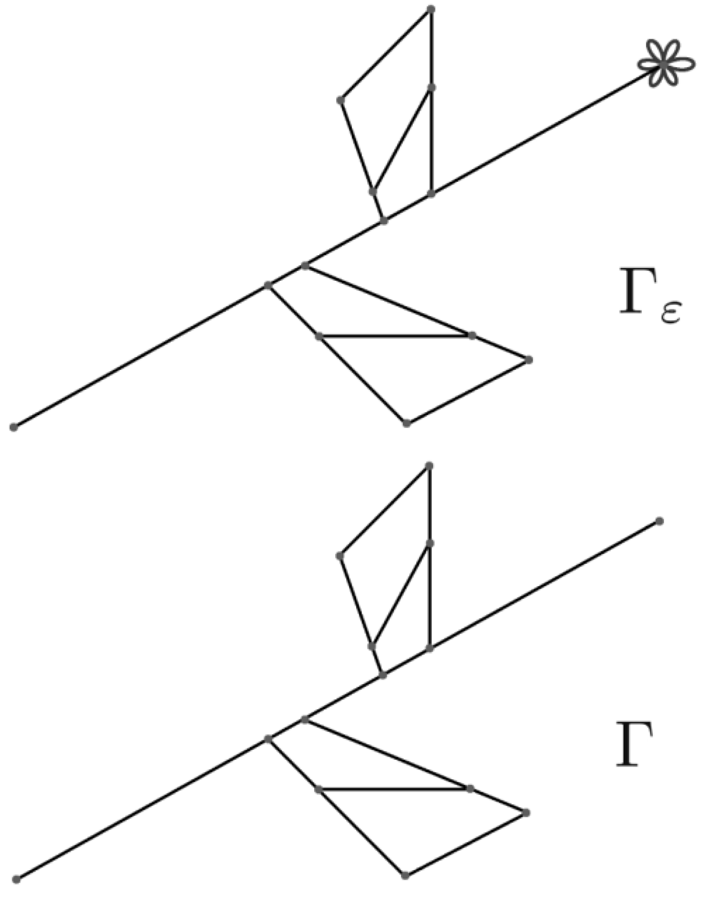
The graph contains small loops attached to the vertex M, whose lengths are proportional to . These loops represent singular perturbations and disappear in the limit leading to the limit graph Γ.
Let the graph Γ be equipped with a real potential that is bounded and continuous. Each small loop is associated with a local variable For these loops, we define scaled potentials of the form where the functions are continuous and real-valued on the intervals The main operator investigated in this paper is the Schrödinger operator acting on the graph . It is defined by the differential expression
where the potential is given by
Here is a small parameter representing the characteristic length of the attached loops.
At the common vertex we impose the standard Kirchhoff matching conditions that ensure the continuity of the function and the conservation of the total flux. These conditions can be written as
and
The first relation expresses the continuity of the wave function at the vertex, while the second one represents the Kirchhoff flux conservation law.
Here, the functions and represent the restrictions of the global function u to the corresponding edges of the graph. The symbols and denote, respectively, the values of these restrictions at the initial and terminal points of the loop . The same interpretation applies to the terms involving the derivatives of , where each derivative is taken in the direction outward from the vertex M. At the remaining vertices of the graph Γ, we impose the standard boundary conditions, ensuring that the operator is self-adjoint in the Hilbert space . Such types of vertex conditions guaranteeing self-adjointness are well described in the general theory of differential operators on graphs (see, for example, [14] (Chapter 1, Subsection 1.4.1, Theorem 1.4.4) and [11] (Lemma 4.1)). The domain of the operator is defined as a subspace of consisting of all functions that satisfy the prescribed boundary conditions at the vertices of the graph . For any metric graph, we denote by the direct sum of the Sobolev spaces taken over all edges e of the graph, that is,
We impose the following key assumption on the potentials . For each the function is such that the boundary value problem
admits a single nontrivial solution. Moreover, this solution satisfies the normalization condition
We denote by another linearly independent solution of the differential equation given in (2). Using the normalization condition (3) and the fact that the Wronskian of two linearly independent solutions of Equation (2) remains constant along the interval, we can select the function in such a way that
The main objective of this work is to investigate the analytic behavior of the resolvent associated with the operator in the limit as In order to present the principal results, we first introduce several auxiliary definitions and notations.
Let the collection of all small loops of the graph be denoted by . The Hilbert space can naturally be regarded as the direct sum
Let be a graph consisting of the edges . In the space we define the contraction operators that map functions from into by the rule
It is straightforward to verify that each operator is bounded and invertible. Moreover, their operator norms satisfy the relations
Throughout the paper, the notation denotes the operator norm of a bounded linear mapping from a Banach space X into a Banach space Y. We introduce the operator
and denote by
the combined mapping acting between the spaces associated with the unscaled and scaled graphs, respectively.
We define two auxiliary operators, denoted by and , acting on the graph Γ and associated with the same differential expression
where V is a real, bounded, and continuous potential on the edges of Γ. At all vertices of the graph, except for the vertex M, we impose the same boundary conditions as those used for the operator . At the distinguished vertex M, the operator is defined by the Dirichlet boundary condition
whereas the operator corresponds to the Neumann condition
The domains of these operators, denoted by and , are the subspaces of consisting of functions that satisfy the respective boundary conditions at all vertices of Γ Both and are self-adjoint operators in due to the imposed boundary conditions (see [11] (Lemma 4.1)).
Let us introduce the restriction operators and which act from the space onto and respectively. These operators are defined by the relations
where and denote the restrictions of a function u, defined on the entire graph to the subgraph Γ and to the loop respectively. It is then convenient to define the combined restriction operator
which maps functions from the space to their restrictions on the subgraph , consisting of all small loops attached to the vertex M.
Since the operators and are self-adjoint, their resolvents , , are well defined for all complex values of such that Im . For such values of , we introduce on the space , a pair of linear operators defined by
here, denotes the identity operator in the space , and the direct sum is taken in accordance with the decomposition . It follows directly from the definitions that the operator acts as a bounded mapping from into while the operator is bounded as an operator from to .
For convenience, we introduce the notation , which will be used in the statement of the main theorem presented below.
Theorem 1.
Let Im . Then the operators and are holomorphic with respect to the small parameter ε. If
then the leading terms of the Taylor expansions of and as are given by
where the direct sum is taken in the sense of the decomposition
If, on the other hand,
then the first terms of the corresponding Taylor series have the following form:
where
Let us analyze the principal result in more detail, starting from the behavior of the operators and . The operator acts on a pair of functions , where is defined on the main graph Γ and f on the loops i. The action is as follows: the component remains unchanged, while in the second component f, the variable is rescaled (contracted), so that the resulting function is defined on the small loops . Hence, we obtain a function belonging to the space . Applying the resolvent to this function and then restricting the result to the subgraph Γ and to the small loops we get the following. The restriction to Γ corresponds precisely to the action of the operator . Similarly, applying the inverse contraction operator to the restriction on the small loops yields the same result as the action of the operator on the pair . Therefore, it is natural to interpret the operators and as the components of the resolvent corresponding to the subgraph Γ and the system of small loops , respectively. This interpretation is supported by the fact that the full resolvent can be reconstructed from its parts via the simple identity
In accordance with the general theory developed in [11], the components of the resolvent associated with operators on graphs containing small edges are analytic with respect to the parameter in the generic situation, that is, when the so-called nonresonance condition A from [11] is fulfilled.
The graph considered in this paper, however, represents a simple instance where this condition is not satisfied. Following the analytical framework proposed in [11], we examine a model graph composed of several loops and a single semi-infinite edge, all joined at a common vertex M. The coordinate along the semi-infinite edge is denoted by , and the entire structure will be referred to as the graph . On this graph, we define a self-adjoint operator acting according to the differential expressions
subject to the Kirchhoff matching condition at the vertex M. The essential spectrum of coincides with the semi-axis . The nonresonance condition A from [11] asserts that there are no eigenvalues embedded at the lower bound of this essential spectrum. However, the framework allows for the existence of a virtual level, which corresponds to a nontrivial solution of the equation on the graph such that takes constant values along the semi-infinite edge.
In the present situation, the nonresonance condition A is clearly violated, since the operator admits exactly n eigenfunctions associated with the lower edge of its essential spectrum. Each of these eigenfunctions coincides with the function on the corresponding loop i and vanishes identically on all other edges of the graph . The boundary conditions for specified in (2)–(3) ensure that the Kirchhoff matching condition at the common vertex M is automatically satisfied. In addition, the operator may also exhibit the presence of a virtual level located at the bottom of the essential spectrum. The criterion for the existence of such a level is precisely the relation given by identity (8). In this resonant case, the associated generalized eigenfunction takes the form on each loop i and equals 1 identically on the semi-infinite edge.
According to Theorem 1, even though the nonresonance condition A is not fulfilled, the operators and nevertheless remain holomorphic with respect to . This constitutes the first key observation derived from our main theorem and demonstrates that the analyticity of these operators is, in fact, a universal feature. Furthermore, the leading term in the Taylor expansion of coincides with that obtained in the standard situation where condition A is satisfied. Specifically, when inequality (6) holds, the operator H does not admit a virtual level, and the leading term corresponds to the resolvent with a Dirichlet condition at the vertex M. Conversely, if equality (8) is valid, a virtual level emerges, and the leading term involves the operator subject to a Neumann condition. These findings are in full agreement with the conclusions of [11] for the nonresonant case: as the small parameter tends to zero, one obtains the Dirichlet condition at M in the presence of a virtual level, and the Neumann condition otherwise.
The second key conclusion derived from Theorem 1 highlights the principal distinction between our results and those established in [11] for the nonresonant case. This difference concerns the behavior of the operator in particular, the structure of the leading term in its Taylor expansion. Specifically, an additional component of the form
appears in the leading term, representing a qualitatively new contribution absent in the nonresonant setting. The additional term is characterized by the projection of f onto the eigenfunctions corresponding to the embedded eigenvalue at zero. It appears in both (7) and (9), indicating that its presence is independent of the existence of a virtual level. In the case where a virtual level is present, an additional term emerges
This term appears in the leading order (see (9)) and is qualitatively distinct from the other term. Specifically, the projection onto the eigenfunctions corresponding to the embedded eigenvalue is determined solely by the function that is, it depends on the graph and the values of the right-hand side on the small loops. Moreover, if the right-hand side vanishes on the finite edges of the subgraph , then the leading term in the Taylor series of the operator is identically zero, and the term associated with the virtual level in (9) also vanishes. A similar property was observed in [11], where the leading terms in the Taylor series for the operators and were entirely determined by the right-hand side on the finite edges. In the present case, however, due to the embedded eigenvalue, an additional term depending solely on arises in the leading term of the Taylor series of . When , only a first-order term remains in the restriction of the resolvent on small loops. This indicates that the resolvent is effectively localized on the small loops. A related phenomenon was previously noted in [2] (Theorem 2), although no statements regarding holomorphy were made there; furthermore, the graph Γ considered was of a very simple, star-shaped structure.
In summary, we conclude the following. For a graph containing small loops, if an embedded eigenvalue exists at the bottom of the essential spectrum of the operator , the holomorphy of the operators and is preserved. The term representing the projection of onto the eigenfunctions corresponding to the embedded eigenvalue appears in the leading term of the Taylor expansion of , indicating an additional localization of the resolvent of on the small loops. The remaining terms in the leading part of the Taylor series of and are analogous to those in the nonresonance case described in [11].
2. Analytic Behaviour of the Resolvent
In this section, we prove Theorem 1. Owing to the simple structure of , specifically the small loops , the resolvent of can be explicitly represented, allowing for a detailed analysis of the operators and .
We select arbitrary functions and and define by and we consider the resolvent equation for the operator :
Focusing on the loop , we introduce the scaled variable . Setting , with we immediately obtain the ordinary differential equation
Since is fixed and is small, the term is correspondingly small.
We denote by the self-adjoint operator in generated by the differential expression
subject to Dirichlet boundary conditions. The domain consists of functions in that vanish at the end points of the interval . Let be the eigenfunction corresponding to the zero eigenvalue. Since this eigenvalue is simple, the standard resolvent expansion of a self-adjoint operator in a neighborhood of an isolated eigenvalue (see, e.g., [15]) applies. Consequently, for sufficiently small , the resolvent admits the representation
where denotes the orthogonal projection onto the eigenfunction in ; its action is given by
The operator is bounded, and its dependence on is holomorphic in a neighborhood of . Moreover, the image of lies entirely in the domain .
We further introduce the notation
We examine the behavior of the fundamental system of solutions to the differential equation
Assuming that the functions and are known for all , Equation (15) can be reformulated, in the usual manner, as a Volterra integral equation of the second kind:
where and are arbitrary constants. The operator is clearly bounded when regarded as a mapping from into . Consequently, the operator , with I denoting the identity operator, is well defined for sufficiently small and depends holomorphically on as an operator . This ensures that Equation (16) has a unique solution in whenever is sufficiently small. We denote by the solution corresponding to and , and by the one associated with and , that is Both functions and depend holomorphically on for sufficiently small values of the parameter, when considered in the -norm. Moreover, they satisfy the identities
Using these observations, the general solution of Equation (11) may be written in the form
We now examine Equation (10) restricted to the subgraph Γ of . On Γ, this equation reduces to the differential problem
supplemented with the prescribed boundary conditions at every vertex of Γ, except at the vertex M. At this vertex the function u is required to satisfy the Kirchhoff condition, modified to account for the presence of the small loop Γ. Because the resolvent is well defined for the chosen value of , the function solves Equation (19) and satisfies all the boundary conditions on Γ, except that it vanishes at the vertex M. Consequently, belongs to the space .
Let be a smooth cut-off function defined on the edge which equals 1 in a small neighborhood of the vertex M and vanishes outside a sufficiently large neighborhood of M. Extend by zero to all other edges of Γ, and introduce
Using the standard mapping properties of the resolvent , one verifies that , satisfies all vertex boundary conditions on Γ except at M, and in addition solves the boundary value problem
We observe that
since, otherwise, (having a nonzero imaginary part) would have to be an eigenvalue of the self-adjoint operator , which is impossible.
Using the known properties of and , consider the function , where is an arbitrary constant. This function lies in the space , solves Equation (19), and satisfies all vertex boundary conditions on the graph Γ except at the vertex M. At M the function w obeys
We seek a solution of Equation (10) in the form
where the functions w and are given by relations (18) and (21).
Due to the previously established properties of these functions, the constructed belongs to the space and satisfies the differential equation
together with all vertex boundary conditions on except at the vertex M. In what follows, we demonstrate that an appropriate choice of the unknowns and ensures that the Kirchhoff condition (1) is fulfilled at M.
Using the first set of identities in (1) together with (21), while also accounting for the boundary conditions satisfied by , we obtain
The second equality in (23) enables us to express each of the quantities and in terms of the other. To proceed, we analyze the asymptotic behavior of the differences , as . It is convenient to present the required properties in the following form.
Lemma 1.
Each of the functions and is holomorphic for sufficiently small values of μ. Moreover, the following relations are valid:
Proof.
The analyticity of all listed functions follows directly from the fact that and depend holomorphically on in the -norm. If we expand in (17) into its Neumann series, we obtain
Using these representations, together with the explicit form of the operator in (16) and the boundary conditions stated in (2)–(4), one directly derives all expansions and identities collected in (25).
From the second relation in (23), we can rewrite the coefficient in terms of as
Using the expansions in (25), one sees that the map
is well-defined for small and is holomorphic in this parameter.
Furthermore, the leading terms of its Taylor expansion are given by
To obtain the second identity, we make use of the Kirchhoff condition (1). Substituting the representation of from (22) and using (21), the definition of the operators , as well as Formula (18), we arrive at
By substituting the obtained formulas for and into the above identity, we arrive at an equation that determines K. Solving this equation yields
where
Using the expansions in (25), we observe that the function Q is holomorphic in , and its Taylor expansion at begins with
To analyze the behavior of the differences for , we multiply the differential equation satisfied by by and integrate by parts twice, making use of the boundary conditions for both and . This yields
Using the last identity together with (28), (24), (26), and (14), we can finally obtain the expressions for , and K. Specifically, we have
and therefore
Since the operator and the functions are holomorphic in the functions are meromorphic in . They can therefore be interpreted as the values of meromorphic bounded linear functionals in , acting on the space . We denote these functionals by the same symbols and K. Namely,
Using Formulas (27) and (29) and inequality (20), we obtain that the functionals K and are holomorphic in , and the first terms of their Taylor expansions satisfy
if condition (6) holds, whereas
if condition (8) holds. Here the remainder terms are understood in the norms of bounded linear functionals on .
Thus, the functions and have been determined, which confirms the validity of the Kirchhoff condition (1). As a result, the function introduced in (22) indeed represents the action of the resolvent on the function f. Using the definitions of the operators and given in (5), we directly obtain . Substituting (12) into (14), then inserting the resulting identity into (18), and taking into account the known properties of the functions and as well as those of the functionals K and , we derive explicit formulas for these operators. Consequently,
where and
From the explicit representations obtained above, it follows that the operators and depend holomorphically on the parameter . Making use of identities (29) and (25), together with the elementary equalities
one can directly check that the leading terms of the Taylor expansions of these operators agree with Formula (7) when condition (6) is satisfied, and with Formula (9) when condition (8) is fulfilled. This completes the proof of the theorem. □
3. Discussion: Comparison with the Nonresonant Case and an Illustrative Example
3.1. Comparison with the Nonresonant Case
We briefly compare the results obtained in the present (resonant) setting with those established previously in the nonresonant case.
In the nonresonant situation, the eigenvalues involved in the asymptotic construction do not satisfy any resonance relations. Consequently, the perturbation procedure proceeds in a regular manner: at each step of the asymptotic expansion, the correction terms are uniquely determined by solving linear problems with nonvanishing spectral gaps. No additional compatibility conditions arise, and the amplitudes corresponding to different modes remain decoupled. In particular, the leading-order term preserves the qualitative structure of the associated linear problem, and the reduced model retains a scalar (or diagonally decoupled) character.
In contrast, in the resonant configuration considered in this paper, certain eigenvalues satisfy resonance relations. As a result, the higher-order equations generate additional solvability (orthogonality) conditions. These conditions lead to a coupled amplitude system governing several interacting modes simultaneously. The asymptotic construction can no longer be performed mode by mode independently, and the structure of the leading-order term is modified by nonlinear interaction effects.
Therefore, unlike the nonresonant case, the resonant regime produces a qualitatively different limiting behavior and alters the structure of the reduced problem. This distinction underlines the mathematical novelty of the present analysis.
3.2. A Simple Illustrative Example
To clarify the abstract construction underlying the main results, we present a simplified model example illustrating the difference between the nonresonant and resonant mechanisms.
Consider the perturbed problem
where L is a linear self-adjoint operator with eigenvalues and and corresponding eigenfunctions and , and is a small parameter. We seek a solution in the form
3.2.1. Nonresonant Case
If , substitution of the expansion and projection onto the eigenspaces generated by and yield independent equations for the amplitudes and . Since the eigenvalues are separated, the associated linear operators are invertible on the orthogonal complements, and no additional compatibility conditions arise. The correction term is uniquely determined, and the construction proceeds in a decoupled manner.
3.2.2. Resonant Case
If , the projection of the higher-order terms onto the resonant eigenspace leads to compatibility conditions of the form
These conditions produce a coupled system for the amplitudes and . The interacting modes must therefore be determined simultaneously, and the reduced problem acquires a genuinely coupled structure. This mechanism reflects, in a simplified form, the phenomenon responsible for the qualitative differences established in the main results of this paper.
4. Conclusions
We have analyzed the resolvent of a Schrödinger operator on a graph with small loops in the resonant regime, where the standard nonresonance condition is violated. The results show that the relevant components of the resolvent admit a holomorphic expansion in the small parameter ϵ, with an additional leading-order term arising from eigenfunctions localized on the shrinking loops. This term reveals a threshold localization effect associated with embedded eigenvalues or virtual levels and highlights the influence of small-scale geometry on the operator.
Although the present work focuses on the resolvent level, the obtained results provide a solid foundation for further investigations of spectral and dynamical properties of quantum graphs with small edges. In particular, they suggest possible extensions to the study of threshold resonances, scattering behavior, and related time-dependent problems. We expect that the approach developed here may be useful in addressing these questions in more general graph settings.
Author Contributions
Software, G.A.; Validation, M.K.; Formal analysis, G.A.; Investigation, M.K.; Data curation, M.K.; Writing—original draft, M.K. and G.A.; Writing—review & editing, M.K. and G.A.; Project administration, M.K. and G.A.; Funding acquisition, M.K. All authors have read and agreed to the published version of the manuscript.
Funding
This research was funded by the Science Committee of the Ministry of Education and Science of the Republic of Kazakhstan (Grant No. AP22685191).
Data Availability Statement
The original contributions presented in this study are included in the article. Further inquiries can be directed to the corresponding author.
Conflicts of Interest
The authors declare no conflict of interest.
References
- Kurasov, P.; Nowaczyk, M. Inverse spectral problem for quantum graphs. J. Phys. A Math. Gen. 2005, 38, 4901–4915. [Google Scholar] [CrossRef] [Scilit]
- Kuchment, P. Quantum graphs: An introduction and a brief survey. Proc. Symp. Pure Math. 2008, 77, 291–314. [Google Scholar]
- Kostrykin, V.; Schrader, R. Kirchhoff’s rule for quantum wires. J. Phys. A Math. Gen. 1999, 32, 595–630. [Google Scholar] [CrossRef] [Scilit]
- Bolte, J.; Endres, S. Trace formulae for quantum graphs. Ann. Henri Poincaré 2009, 10, 189–223. [Google Scholar] [CrossRef] [Scilit]
- Gnutzmann, S.; Smilansky, U. Quantum graphs: Applications to quantum chaos and universal spectral statistics. Adv. Phys. 2006, 55, 527–625. [Google Scholar] [CrossRef] [Scilit]
- Post, O. Spectral Analysis on Graph-like Spaces; Lecture Notes in Mathematics; Springer: Berlin/Heidelberg, Germany, 2012. [Google Scholar]
- Kuchment, P.; Zeng, H. Asymptotics of spectra of Neumann Laplacians on thin domains. Contemp. Math. 2003, 327, 199–213. [Google Scholar]
- Berkolaiko, G.; Keating, J. Two-point spectral correlations for star graphs. J. Phys. A Math. Gen. 1999, 32, 7827–7841. [Google Scholar] [CrossRef] [Scilit]
- Friedlander, L. Genericity of simple eigenvalues for a metric graph. Israel J. Math. 2005, 146, 149–156. [Google Scholar] [CrossRef] [Scilit]
- Molchanov, S.; Vainberg, B. Scattering solutions in networks of thin fibers: Small diameter asymptotics. Commun. Math. Phys. 2007, 273, 533–559. [Google Scholar] [CrossRef] [Scilit]
- Exner, T.; Post, O. Convergence of spectra of graph-like thin manifolds. J. Geom. Phys. 2005, 54, 77–115. [Google Scholar] [CrossRef] [Scilit]
- Kuchment, P.; Post, O. On the spectra of carbon nano-structures. Commun. Math. Phys. 2007, 275, 805–826. [Google Scholar] [CrossRef] [Scilit]
- Alon, L.; Band, R.; Berkolaiko, G. Universality of nodal count distribution in large metric graphs. Exp. Math. 2022, 33, 301–335. [Google Scholar] [CrossRef] [Scilit]
- Barra, F.; Gaspard, P. Transport and dynamics on open quantum graphs. Phys. Rev. E 2002, 65, 016205. [Google Scholar] [CrossRef] [Scilit] [PubMed]
- Post, O. Spectral convergence of quasi-one-dimensional spaces. Ann. Henri Poincaré 2006, 7, 933–973. [Google Scholar] [CrossRef] [Scilit]
Disclaimer/Publisher’s Note: The statements, opinions and data contained in all publications are solely those of the individual author(s) and contributor(s) and not of MDPI and/or the editor(s). MDPI and/or the editor(s) disclaim responsibility for any injury to people or property resulting from any ideas, methods, instructions or products referred to in the content. |
© 2026 by the authors. Licensee MDPI, Basel, Switzerland. This article is an open access article distributed under the terms and conditions of the Creative Commons Attribution (CC BY) license.