Information-Geometric Models in Data Analysis and Physics II

Abstract

This paper continues the development of information-geometric models for data analysis and physics by focusing on their formulation and interpretation through variational principles. Building on the geometric framework introduced previously, we investigate how fundamental variational structures—such as information-theoretic functionals—naturally encode the laws of nature. In the first manuscript, we showed that a wide class of physical problems can be expressed as constrained variational problems on spaces of probability distributions, leading to geodesic flows, gradient dynamics, and generalized Hamiltonian formulations on statistical manifolds. In this second part, we extend the variational formalism by utilizing an extended metric, clarifying the geometric origin of the dynamical equations commonly used in modern physics and providing a coherent interpretation of physical laws in terms of information optimization. By emphasizing variational foundations, this paper strengthens the conceptual and mathematical links between information geometry, data analysis, and physics, and it provides a flexible framework for extending geometric methods to complex, high-dimensional, and dynamical systems.

1. Introduction

In recent years, the interaction between data and geometry has surged as a transformative frontier in both information science and physics. The concept of information-induced geometries suggests that the structure and behavior of physical systems can be understood and modeled at a fundamental level through geometric frameworks informed by data-driven insights. This innovative approach not only opens new pathways for analyzing complex datasets but also has significant implications for our understanding of the universe’s very fabric. By integrating principles from information theory, differential geometry, and quantum physics, we aim to develop methods that revolutionize data analysis and deepen our understanding of physical phenomena, paving the way for breakthroughs across theoretical insights and practical applications.

Building upon this conceptual foundation, we introduced a robust mathematical framework that leverages advanced geometric and statistical techniques to analyze data residing on Riemannian manifolds [1]. Central to our approach are methods that respect the intrinsic curvature and nonlinear structure of manifold data, such as flow lines of gradient vector fields, exponential and logarithmic maps, and kernel-based principal component analysis (PCA). These tools facilitate faithful, low-dimensional representations and the insightful visualization of complex data structures, capturing both the local and global geometric relationships that are critical for understanding the underlying phenomena. By integrating these geometric insights with an information-theoretic perspective, our framework aims to uncover the mechanisms through which information manifests in physical systems, advancing the notion that informational principles fundamentally shape the universe’s fabric. This interdisciplinary approach offers promising avenues for both theoretical explorations and practical applications in data science, physics, and beyond.

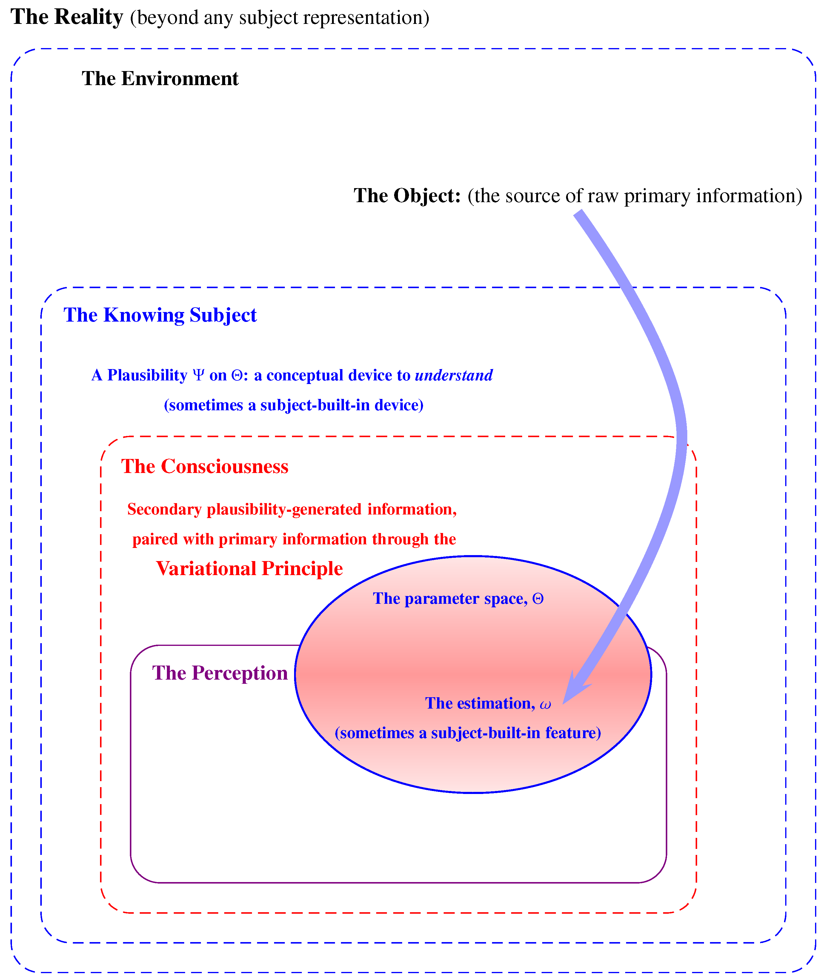
The idea that information is a fundamental building block of the universe is gaining significant traction in theoretical physics and mathematics [2,3,4]. This enlightening perspective suggests that beyond the realms of matter and energy, information intricately weaves the very fabric of reality, shaping the structure and dynamics of everything from subatomic particles to vast cosmic phenomena. Recognizing information as a core component unlocks deep insights into the nature of physical laws, the origins of the universe, and the intricate interconnectedness of all existence. This paradigm shift not only enhances our understanding but also paves the way for groundbreaking explorations into the most profound enigmas of the universe (see Figure 1).

This paper is poised to advance a robust mathematical framework and pioneering conceptual tools that delve into the profound relationship between information and the physical universe. By formalizing the principles governing information processing and its manifestation in physical systems, we aim to uncover the intricate mechanisms by which information may emerge from or be embedded in the fundamental laws of physics [5,6]. This approach not only establishes strong connections between abstract informational concepts and concrete physical models but also provides a solid foundation for investigating how information-theoretic principles could transform our understanding and inspire the development of new theories of reality [7,8].

By representing parametric models through complex-valued functions that encapsulate both magnitude and phase, we construct a Riemannian manifold structure on the parameter space informed by divergence functions and complex model functions. This approach generalizes classical information geometry by incorporating phase information relevant to physical phenomena, such as quantum states and wave propagation. We explore how these geometric structures facilitate the analysis of model sensitivities, estimation procedures, and information encoding with particular emphasis on invariance properties and their implications for physical and statistical inference [9].

In particular, we further develop variational principles rooted in the geometric formalism with novel constraints, yielding differential equations reminiscent of quantum wave equations that govern optimal plausibility functions representing observer beliefs or physical states. Using an illustrative example with Gaussian-modulated wave functions, we demonstrate the applicability of this framework to models with deep physical significance.

Our results establish a foundational bridge between information theory, differential geometry, and physics, offering new tools for modeling, analyzing, and interpreting complex systems. This interdisciplinary integration opens avenues for exploring the informational fabric of the universe, providing insights into the emergence of physical laws from informational principles and fostering the development of novel theoretical and experimental paradigms.

2. Materials and Methods

As in [1], we assume that all relevant aspects of the observation process—whether determined by the object, the subject, the environment, or any combination thereof—can be adequately described by elements of the parameter space $\mathrm{\Theta }$ through a suitable family of complex-valued maps, which will be introduced below. To motivate this framework, we first consider a measure space $(\chi ,\mathcal{A},\nu )$, where $\chi$ is an arbitrary set (the sample space), $\mathcal{A}$ is a $\sigma$–algebra of subsets of $\chi$, and $\nu$ is a positive $\sigma$–finite measure on the measurable space $(\chi ,\mathcal{A})$. Let $\mathrm{\Theta }$ be a manifold and let $p:\chi \times \mathrm{\Theta }\to \mathbb{R}$ be a measurable function such that for each $\mathit{\theta }\in \mathrm{\Theta }$, $P_{\mathit{\theta }}\left(dx\right)=p(x,\mathit{\theta })\nu \left(dx\right)$ defines a probability measure on $(\chi ,\mathcal{A})$. This constitutes the underlying statistical model. Each point of the manifold $\mathrm{\Theta }$ represents, potentially, a distinct information source from which sample data are obtained under independence assumptions. Let $\mathit{x}\in {\chi }^n$, say $\mathit{x}=(x_1,\dots ,x_n)$, denote a sample with values in $\chi$. For fixed $\mathit{\theta }$, the joint density with respect to the product measure ${\nu }^{\otimes n}$ is given by $\tilde{p}(\mathit{x},\mathit{\theta })={\prod }_{i=1}^{n}p(x_i,\mathit{\theta }).$ The sample is assumed to provide a statistically consistent estimator $T\left(\mathit{x}\right)=T(x_1,\dots ,x_n)$ of the true parameter $\mathit{\theta }\in \mathrm{\Theta }$ characterizing the information source under study.

Fix $\mathit{\theta }\in \mathrm{\Theta }$ and an estimator T. The mapping T induces a probability measure on $(\mathrm{\Theta },\mathcal{B}(\mathrm{\Theta }\left)\right)$ defined by $P_{\mathit{\theta }}^T\left(B\right)=P_{\mathit{\theta }}\left(T^{-1}\left(B\right)\right),$ for any Borel set $B\in \mathcal{B}\left(\mathrm{\Theta }\right)$, where $\mathcal{B}\left(\mathrm{\Theta }\right)$ is the Borel $\sigma$–algebra generated by the open sets of the manifold $\mathrm{\Theta }$. Under appropriate regularity conditions, this induced measure admits a density with respect to a conveniently defined measure on the manifold $\mathrm{\Theta }$, $d\mu$, namely $f(\mathit{\omega },\mathit{\theta })={\displaystyle \frac{d{P}_{\mathit{\theta }}^T}{d\mu }}\left(\mathit{\omega }\right),$ which is the Radon–Nikodym derivative of $P_{\mathit{\theta }}^T$ with respect to $d\mu$. In what follows, we focus on this probability density on $\mathrm{\Theta }$, or more precisely, on a not necessarily real square root of it, in contrast with the standard real-valued framework of information geometry. To investigate the behavior and structural properties of information sources, we introduce the following notion.

A regular parametric family of functions ${\mathcal{F}}_{\mathrm{\Theta }}$ is defined as a family of measurable maps $h:\mathrm{\Theta }\times \mathrm{\Theta }⟶\mathbb{C},$ which admit a complex exponential representation $h(\mathit{\omega },\mathit{\theta })=r(\mathit{\omega },\mathit{\theta }),e^{i\zeta (\mathit{\omega },\mathit{\theta })},$ where $r(\mathit{\omega },\mathit{\theta })\ge 0$ and $\zeta (\mathit{\omega },\mathit{\theta })$ are real-valued functions representing, respectively, the modulus and the argument of $h(\mathit{\omega },\mathit{\theta })$. This construction generalizes the classical square-root embedding of statistical models by allowing $h(\mathit{\omega },\mathit{\theta })=r(\mathit{\omega },\mathit{\theta })e^{i\zeta (\mathit{\omega },\mathit{\theta })}$, where $f(\omega ,\theta )$ is a probability density. The statistical model is completely determined by ${\left|h\right|}^2$, whereas the phase function $\zeta$ provides an additional geometric degree of freedom. By multiplying the density by a scalar field on $\mathrm{\Theta }$ prior to taking the square root, one may assume without loss of generality that the phase $\zeta$ is independent of the choice of reference measure. For each fixed $\mathit{\theta }\in \mathrm{\Theta }$, the squared modulus $r^2(\mathit{\omega },\mathit{\theta })=h(\mathit{\omega },\mathit{\theta })\overline{h(\mathit{\omega },\mathit{\theta })}$ is required to be a probability density with respect to $d\mu$; that is, $P_{\mathit{\theta }}^T\left(d\mathit{\omega }\right)=r^2(\mathit{\omega },\mathit{\theta })\mu \left(d\mathit{\omega }\right)$ defines a probability measure on $(\mathrm{\Theta },\mathcal{B}(\mathrm{\Theta }\left)\right)$ for all $\mathit{\theta }\in \mathrm{\Theta }$.

Although the probability measure $P_{\mathit{\theta }}^T$ is independent of the particular choice of reference measure, the function $r(·,\mathit{\theta })$ depends on $d\mu$. Indeed, if $\widehat{\mu }$ is another reference measure such that $d\mu /d\widehat{\mu }=\mathfrak{q}$ for some positive measurable function $\mathfrak{q}$, then by the Radon–Nikodym theorem, $P_{\mathit{\theta }}^T\left(d\mathit{\omega }\right)=r^2(\mathit{\omega },\mathit{\theta })\mathfrak{q}\left(\mathit{\omega }\right)\mu \left(d\mathit{\omega }\right)={\widehat{r}}^2(\mathit{\omega },\mathit{\theta })\widehat{\mu }\left(d\mathit{\omega }\right)$, where $\widehat{r}(\mathit{\omega },\mathit{\theta })=r(\mathit{\omega },\mathit{\theta }),\sqrt{\mathfrak{q}\left(\mathit{\omega }\right)}.$ This expression makes explicit the dependence of the modulus r on the chosen reference measure.

Throughout, we implicitly assume the regularity conditions required for subsequent developments, including sufficient smoothness with respect to $\mathit{\theta }$ and the assumption that the closure of the set on which $r(·,\mathit{\theta })$ is strictly positive does not depend on $\mathit{\theta }$. We shall refer to $\mu$ as the reference measure, to h as the model function, and to $f(\mathit{\omega },\mathit{\theta })=r^2(\mathit{\omega },\mathit{\theta })$ as the model density.

2.1. The Riemannian Structure on the Parameter Space

The exploration of Riemannian structures on parameter spaces provides a profound geometric perspective on models and their underlying function spaces. By endowing these spaces with a Riemannian metric, we can investigate the intrinsic geometric properties that influence model behavior, estimation, and inference. Such a perspective enables a more nuanced understanding of the parameter space’s complexity and curvature, offering insights that extend beyond traditional Euclidean approaches.

Letting $L^2(\mathrm{\Theta },\mu )$ be the Hilbert space of these complex-valued measurable functions q in $\mathrm{\Theta }$ such that the Lebesgue integral ${\int }_{\mathrm{\Theta }}{\left|q\left(\mathit{\omega }\right)\right|}^2\mu \left(d\mathit{\omega }\right)<\infty$, where $\left|z\right|=\sqrt{z\overline{z}},z\in \mathbb{C}$, if we denote by $D^2$ the square of the Hilbert distance

$$D^2(p,q)={\int }_{\mathrm{\Theta }}{|p\left(\mathit{\omega }\right)-q\left(\mathit{\omega }\right)|}^2\mu \left(d\mathit{\omega }\right),$$

(1)

once given the model function $h(·,\mathit{\theta })$ of a parametric family, ${\mathcal{F}}_{\mathrm{\Theta }}$, since these functions are naturally identifiable with elements of $L^2(\mathrm{\Theta },\mu )$, we are able to build the function

$$\begin{array}{cc}\hfill {\delta }_{\kappa }^2(\mathit{\gamma },\mathit{\theta })& ={\kappa }^2{D}^2(h(·,\mathit{\gamma }),h(·,\mathit{\theta }))={\kappa }^2{\int }_{\mathrm{\Theta }}{|h(\mathit{\omega },\mathit{\gamma })-h(\mathit{\omega },\mathit{\theta })|}^2\mu \left(d\mathit{\omega }\right)\hfill \\ & ={\kappa }^2\left(2-{\int }_{\mathrm{\Theta }}\left(h(\mathit{\omega },\mathit{\gamma })\overline{h(\mathit{\omega },\mathit{\theta })}+h(\mathit{\omega },\mathit{\theta })\overline{h(\mathit{\omega },\mathit{\gamma })}\right)\mu \left(d\mathit{\omega }\right)\right),\hfill \end{array}$$

(2)

where $\kappa >0$ is a positive constant which determines the units of the dissimilarity measure ${\delta }_{\kappa }^2$ on $\mathrm{\Theta }$, and when $\mathit{\gamma }=\mathit{\theta }$, we have taken into account ${\int }_{\mathrm{\Theta }}h(\mathit{\omega },\mathit{\theta })\overline{h(\mathit{\omega },\mathit{\theta })}\mu \left(d\mathit{\omega }\right)={\int }_{\mathrm{\Theta }}{r}^2(\mathit{\omega },\mathit{\theta })\mu \left(d\mathit{\omega }\right)={\int }_{\mathrm{\Theta }}f(\mathit{\omega },\mathit{\theta })\mu \left(d\mathit{\omega }\right)=1\forall \mathit{\theta }\in \mathrm{\Theta }$ and therefore ${\delta }_{\kappa }^2(\mathit{\theta },\mathit{\theta })=0$. Notice that since $\left|h\right|=|\overline{h}|=r$, if we change the reference measure $\mu$ to $\nu$ accordingly, r changes to $\widehat{r}$, and when we integrate (2) now with respect to $\nu$, we find that ${\delta }_{\kappa }^2(\mathit{\gamma },\mathit{\theta })$ remains invariant.

We are going to consider the Riemannian metric induced in $\mathrm{\Theta }$ by ${\delta }_{\kappa }^2$, following the same basic ideas of [10]. If we define $d_{\kappa ,\mathit{\theta }}^2\left(\mathit{\gamma }\right)={\delta }_{\kappa }^2(\mathit{\gamma },\mathit{\theta })$, we will have $d_{\kappa ,\mathit{\theta }}^2\left(\mathit{\theta }\right)=0$, and taking into account that the Jacobian of $d_{\kappa ,\mathit{\theta }}^2\left(\mathit{\gamma }\right)$ in $\mathit{\gamma }=\mathit{\theta }$ is also null, since the function has an absolute minimum at $\mathit{\theta }$, the second-order expansion of $d_{\kappa ,\mathit{\theta }}^2\left(\mathit{\gamma }\right)$ at $\mathit{\theta }$ will be given by its Hessian at $\mathit{\theta }$, ${\left(d_{\kappa ,\mathit{\theta }}^2\left(\mathit{\theta }\right)\right)}^{″}={\left({\left.{\displaystyle \frac{{\partial }^2{d}_{\kappa ,\mathit{\theta }}^2}{\partial {\gamma }^i\partial {\gamma }^j}}\right|}_{\mathit{\gamma }=\mathit{\theta }}\right)}_{(m\times m)}$, which will be positive definite or semidefinite. Moreover, the Hessian components at $\mathit{\gamma }=\mathit{\theta }$ are the components of a second-order covariant symmetric tensor at each tangent space $T_{\mathit{\theta }}\mathrm{\Theta }$, see [1] for details, in which tensor may be used to define a Riemannian metric in $\mathrm{\Theta }$ with fundamental tensor

$$g_{ij}\left(\mathit{\theta }\right)={\displaystyle \frac{1}{2}}{\displaystyle \frac{{\partial }^2{d}_{\kappa ,\mathit{\theta }}^2}{\partial {\gamma }^i\partial {\gamma }^j}}{|}_{\mathit{\gamma }=\mathit{\theta }}i,j=1,\dots ,m,$$

(3)

i.e., the components of the metric tensor will be equal to one half times the second partial derivatives of the function $d_{\kappa ,\mathit{\theta }}^2$, and the line element corresponding to the above-mentioned induced Riemannian metric, under $\mathit{\theta }=({\theta }^1,\dots ,{\theta }^m)$, is given through its square by

$$d{s}^2=\sum _{i=1}^m\sum _{j=1}^m{g}_{ij}\left(\mathit{\theta }\right)d{\theta }^{i}d{\theta }^j.$$

(4)

This formulation is typical in classical information geometry, where the metric is derived from second derivatives of divergence functions or similar measures.

If we express the complex-valued function $h(·,\mathit{\theta })$ in their exponential form, that is, $h(·,\mathit{\theta })=r(·,,\mathit{\theta })e^{i\zeta (·,\mathit{\theta })}$ for a convenient real-valued function $\zeta$ of $(·,\mathit{\theta })$, from (2), taking into account that if $z=r{e}^{i\zeta }$ then $\overline{z}=r{e}^{-i\zeta }$, we obtain after some laborious but straightforward computations at the point $\mathit{\gamma }=\mathit{\theta }$, and we have

$$\begin{array}{cc}\hfill {\left.{\displaystyle \frac{1}{2}}{\displaystyle \frac{{\partial }^2{d}_{\kappa ,\mathit{\theta }}^2}{\partial {\gamma }^{\beta }\partial {\gamma }^{\alpha }}}\right|}_{\mathit{\gamma }=\mathit{\theta }}=& -{\kappa }^2\left({\int }_{\mathrm{\Theta }}\right({\left.{\displaystyle \frac{{\partial }^{2}r}{\partial {\gamma }^{\beta }\partial {\gamma }^{\alpha }}}(\mathit{\omega },\mathit{\gamma })\right|}_{\mathit{\gamma }=\mathit{\theta }}r(\mathit{\omega },\mathit{\theta })\hfill \\ \hfill & -r^2(\mathit{\omega },\mathit{\theta }){\left.{\displaystyle \frac{\partial \zeta }{\partial {\gamma }^{\alpha }}}(\mathit{\omega },\mathit{\gamma })\right|}_{\mathit{\gamma }=\mathit{\theta }}{\left.{\displaystyle \frac{\partial \zeta }{\partial {\gamma }^{\beta }}}(\mathit{\omega },\mathit{\gamma })\right|}_{\mathit{\gamma }=\mathit{\theta }}\left)\mu \left(d\mathit{\omega }\right)\right),\hfill \end{array}$$

(5)

see [1], but if we take into account that $r(\mathit{\omega },\mathit{\theta })=\sqrt{f(\mathit{\omega },\mathit{\theta })}$ is the real square root of a probability density with respect to the reference measure $\mu$, we can express (5) as

$$\begin{array}{cc}\hfill {\left.{\displaystyle \frac{1}{2}}{\displaystyle \frac{{\partial }^2{d}_{\kappa ,\mathit{\theta }}^2}{\partial {\gamma }^{\beta }\partial {\gamma }^{\alpha }}}\right|}_{\mathit{\gamma }=\mathit{\theta }}=& {\displaystyle \frac{{\kappa }^2}{4}}{\int }_{\mathrm{\Theta }}({\left.{\displaystyle \frac{\partial lnf}{\partial {\gamma }^{\beta }}}(\mathit{\omega },\mathit{\gamma })\right|}_{\mathit{\gamma }=\mathit{\theta }}{\left.{\displaystyle \frac{\partial lnf}{\partial {\gamma }^{\alpha }}}(\mathit{\omega },\mathit{\gamma })\right|}_{\mathit{\gamma }=\mathit{\theta }}f(\mathit{\omega },\mathit{\theta })\hfill \\ \hfill -& {\left.2{\displaystyle \frac{{\partial }^{2}f}{\partial {\gamma }^{\beta }\partial {\gamma }^{\alpha }}}(\mathit{\omega },\mathit{\gamma })\right|}_{\mathit{\gamma }=\mathit{\theta }}+4f(\mathit{\omega },\mathit{\theta }){\left.{\displaystyle \frac{\partial \zeta }{\partial {\gamma }^{\alpha }}}(\mathit{\omega },\mathit{\gamma })\right|}_{\mathit{\gamma }=\mathit{\theta }}{\left.{\displaystyle \frac{\partial \zeta }{\partial {\gamma }^{\beta }}}(\mathit{\omega },\mathit{\gamma })\right|}_{\mathit{\gamma }=\mathit{\theta }})\mu \left(d\mathit{\omega }\right)\hfill \\ \hfill =& {\displaystyle \frac{{\kappa }^2}{4}}({\int }_{\mathrm{\Theta }}{\left.{\displaystyle \frac{\partial lnf}{\partial {\gamma }^{\beta }}}(\mathit{\omega },\mathit{\gamma })\right|}_{\mathit{\gamma }=\mathit{\theta }}{\left.{\displaystyle \frac{\partial lnf}{\partial {\gamma }^{\alpha }}}(\mathit{\omega },\mathit{\theta })\right|}_{\mathit{\gamma }=\mathit{\theta }}f(\mathit{\omega },\mathit{\theta })\mu \left(d\mathit{\omega }\right)\hfill \\ \hfill +& 4{\int }_{\mathrm{\Theta }}{\left.{\displaystyle \frac{\partial \zeta }{\partial {\gamma }^{\alpha }}}(\mathit{\omega },\mathit{\gamma })\right|}_{\mathit{\gamma }=\mathit{\theta }}{\left.{\displaystyle \frac{\partial \zeta }{\partial {\gamma }^{\beta }}}(\mathit{\omega },\mathit{\gamma })\right|}_{\mathit{\gamma }=\mathit{\theta }}f(\mathit{\omega },\mathit{\theta })\mu \left(d\mathit{\omega }\right)).\hfill \end{array}$$

(6)

Moreover, let $\mathcal{I}=\left(i_{\alpha \beta }\right)$ be the $(m\times m)$ Fisher information matrix; for more information refer to the original work by Fisher (1922) [11], corresponding to the density of the model, that is, $i_{\alpha \beta }={\int }_{\mathrm{\Theta }}{\displaystyle \frac{\partial lnf}{\partial {\theta }^{\alpha }}}{\displaystyle \frac{\partial lnf}{\partial {\theta }^{\beta }}}fd\mu$ and additionally define

$${\varkappa }_{\alpha \beta }\left(\mathit{\theta }\right)=4{\int }_{\mathrm{\Theta }}{\left.{\displaystyle \frac{\partial \zeta }{\partial {\gamma }^{\alpha }}}(\mathit{\omega },\mathit{\gamma })\right|}_{\mathit{\gamma }=\mathit{\theta }}{\left.{\displaystyle \frac{\partial \zeta }{\partial {\gamma }^{\beta }}}(\mathit{\omega },\mathit{\gamma })\right|}_{\mathit{\gamma }=\mathit{\theta }}f(\mathit{\omega },\mathit{\theta })\mu \left(d\mathit{\omega }\right),$$

(7)

we obtain that the fundamental tensor of $\mathrm{\Theta }$, (3), converting it as a Riemannian manifold, is equal to

$$g_{\alpha \beta }\left(\mathit{\theta }\right)={\displaystyle \frac{{\kappa }^2}{4}}\left(i_{\alpha \beta }\left(\mathit{\theta }\right)+{\varkappa }_{\alpha \beta }\left(\mathit{\theta }\right)\right),$$

(8)

and the Riemannian metric, using repeated index summation convention, can also be expressed as

$$d{s}^2=g_{\alpha \beta }d{\theta }^{\alpha }d{\theta }^{\beta }={\displaystyle \frac{{\kappa }^2}{4}}\left(i_{\alpha \beta }d{\theta }^{\alpha }d{\theta }^{\beta }+{\varkappa }_{\alpha \beta }d{\theta }^{\alpha }d{\theta }^{\beta }\right)={\displaystyle \frac{{\kappa }^2}{4}}\left(d{s}_I^2+d{s}_A^2\right),$$

(9)

where $d{s}_I^2$ is the information metric and $d{s}_A^2$ is a metric specifically related to the imaginary part of the function that defines the model. Observe that locally, the Riemannian metric induced in $\mathrm{\Theta }$ is the distance induced by the Hilbert metric structure in $L^2(\mathrm{\Theta },d\mu )$ on a radius 2 sphere and coincides, when $\kappa =2$, with the information metric when $\zeta$ is constant. More results on the information metric can be found in [10,12,13], among others.

Please note that while we assume that all properties of an information source are determined by $\mathit{\theta }$ or $h(·,\mathit{\theta })$, the exact value of $\mathit{\theta }$ has to be estimated from the data generated by the source. Although we assume that these data can remain partially hidden, it should still allow a reasonably good estimate of both $\mathit{\theta }$ and $h(·,\mathit{\theta })$.

2.2. Physical Applications

In the first manuscript [1], we introduced the concept of extended information, codified by the estimation $\mathit{\omega }$, obtained from an information source, of the true parameter $\mathit{\theta }$, which is information relative to this true value of the parameter, and referred to an arbitrary point ${\mathit{\theta }}_0$, as

$$\begin{array}{cc}\hfill I_{\mathit{\omega }}\left(\mathit{\theta }\right)& =-\iota \left(logh(\mathit{\omega },\mathit{\theta })-logh(\mathit{\omega },{\mathit{\theta }}_0)\right)\hfill \\ & =-\iota \left({\displaystyle \frac{1}{2}}ln{r}^2(\mathit{\omega },\mathit{\theta })+i\zeta (\mathit{\omega },\mathit{\theta })-{\displaystyle \frac{1}{2}}ln{r}^2(\mathit{\omega },{\mathit{\theta }}_0)-i\zeta (\mathit{\omega },{\mathit{\theta }}_0)\right),\hfill \end{array}$$

(10)

where log denotes a version of the complex logarithm defined to satisfy $logh(\mathit{\omega },\mathit{\theta })=lnr(\mathit{\omega },\mathit{\theta })+i\zeta (\mathit{\omega },\mathit{\theta })$, ln being the standard natural logarithm, and $\iota$ is a constant that determines the units of information with which we will work. The implicit dependence of (10) on ${\mathit{\theta }}_0$ is omitted from the notation, since its choice will not play any further role when we calculate its gradient in the parametric space. Additionally, (10) will remain invariant under appropriate data changes and, fixed $\mathit{\omega }$ is also invariant under coordinate changes in the parametric manifold, since it is a scalar field on $\mathrm{\Theta }$.

The information provided by a source external to the observer is represented within him, allowing him to increase his understanding of the objects. Although we can consider different levels and types of the said representation, we will focus on two critical aspects: the parameter space with its natural extended information geometry and the observer’s ability to construct a plausibility regarding the true value of the parameter, $\mathrm{\Psi }$, in the parameter space $\mathrm{\Theta }$, once given a particular estimation of the true parameter, essentially a complex square root of a kind of subjective conditional probability density with respect to the Riemannian volume, which is induced by the information metric over the parameter space, $\mathrm{\Theta }$, up to a normalization constant. Specifically, we shall write at the beginning

$${\int }_{\mathrm{\Theta }}\mathrm{\Psi }\left(\mathit{\theta }\right)\overline{\mathrm{\Psi }\left(\mathit{\theta }\right)}V\left(d\mathit{\theta }\right)=a>0,$$

(11)

although we shall be particularly interested in the case $a=1$. Observe that in (11), we are integrating with respect to the Riemannian measure defined in (3), and therefore this expression is invariant under coordinate changes. Furthermore, if we intend to define on the parametric manifold a probability, interpretable as a plausibility about the true value of the parameter, we can take the function $\mathrm{\Psi }\overline{\mathrm{\Psi }}$ as the Radon–Nikodym derivative of said probability with respect to the Riemannian volume, which is also a measure in the same parameter space. Both measures are independent of the coordinate system used and, therefore, $\mathrm{\Psi }\overline{\mathrm{\Psi }}$ will be an invariant scalar field on the parametric manifold $\mathrm{\Theta }$. Then, if we let $\psi =\left|\mathrm{\Psi }\right|$, we can simply define the information encoded by the subjective plausibility $\mathrm{\Psi }\left(\mathit{\theta }\right)=\psi \left(\mathit{\theta }\right)e^{i\varrho \left(\mathit{\theta }\right)}$ on the parameter space $\mathrm{\Theta }$ relative to the true parameter $\mathit{\theta }$ as

$$\Lambda \left(\mathit{\theta }\right)=-\iota log\left(\mathrm{\Psi }\left(\mathit{\theta }\right)\right)=-\iota \left({\displaystyle \frac{1}{2}}ln{\psi }^2\left(\mathit{\theta }\right)+i\varrho \left(\mathit{\theta }\right)\right).$$

(12)

This quantity (12) remains also invariant under coordinate changes in the parametric manifold, being another scalar field in $\mathrm{\Theta }$; see also [14].

The Variational Principle

In this context, trusting that many of the abilities of the observer have been efficiently shaped by natural selection in the process of biological evolution, we propose that the subjective information mentioned above adjusts in some way to the information provided by the source and in particular satisfying the following variational principle; see also [14]. However, in this paper, we are going to solve a slightly more flexible variational principle considering that given $\omega$, $\mathrm{\Psi }$ vanishes outside the submanifold ${\mathrm{\Theta }}_{\omega }\subset \mathrm{\Theta }$, which is a submanifold that is possibly dependent on $\omega$ but eventually could be the whole $\mathrm{\Theta }$, and, therefore, the functional to be minimized or at least make stationary will become the following

$$\Omega \left(\mathrm{\Psi }\right)={\int }_{{\mathrm{\Theta }}_{\omega }}{|\mathrm{grad}{I}_{\mathit{\omega }}\left(\mathit{\theta }\right)-\mathrm{grad}\Lambda \left(\mathit{\theta }\right)|}^2\mathrm{\Psi }\left(\mathit{\theta }\right)\overline{\mathrm{\Psi }\left(\mathit{\theta }\right)}V\left(d\mathit{\theta }\right),$$

(13)

subject to the constraint (11), which may be written as, subject to the constraint

$${\int }_{{\mathrm{\Theta }}_{\omega }}{\psi }^2\left(\mathit{\theta }\right)dV=a>0,$$

(14)

and, potentially, to another constraint

$${\int }_{{\mathrm{\Theta }}_{\omega }}H\left(\mathit{\theta }\right){\psi }^2\left(\mathit{\theta }\right)V\left(d\mathit{\theta }\right)=b.$$

(15)

This additional constraint is intended as a basic first attempt to model the subject’s limitations in apprehending the object of knowledge. The subject seeks to describe the object by exploiting as fully as possible the information generated by it, as quantified in (10). However, this exploitation—formulated in terms of the variational principle (13)—cannot be achieved without a bound; rather, it can only be partially attained. This limitation arises fundamentally from the constraints inherent in the subject, which are precisely represented by the additional constraint aforementioned (15).

Moreover, it will also be assumed that $\mathrm{\Psi }$ and its gradient $\mathrm{grad}\mathrm{\Psi }$ vanish at the boundary $\partial {\mathrm{\Theta }}_{\omega }$ or at infinity, which is the way to model that we have strong reasons to believe that the true parameter $\mathit{\theta }$ should belong far from the boundary and clearly inside of ${\mathrm{\Theta }}_{\omega }$. Notice that the functional $\Omega$ is equal to the expected value corresponding to the probability in $\mathrm{\Theta }$ given by the density $\mathrm{\Psi }\overline{\mathrm{\Psi }}$ with respect to the Riemannian volume induced by the metric (9), $V\left(d\mathit{\theta }\right)$, of the square of the norm, corresponding to the vector field $\mathrm{grad}{I}_{\mathit{\omega }}\left(\mathit{\theta }\right)$ minus $\mathrm{grad}\Lambda \left(\mathit{\theta }\right)$.

Observe that the difference between the gradients $\mathrm{grad}{I}_{\mathit{\omega }}\left(\mathit{\theta }\right)$ and $\mathrm{grad}\Lambda \left(\mathit{\theta }\right)$ is a complexified vector field in a Riemannian manifold. If we denote by $r_{\omega }\left(\mathit{\theta }\right)=r(\omega ,\mathit{\theta })$ and ${\zeta }_{\omega }=\zeta (\omega ,\mathit{\theta })$ for a specific $\omega$, and omitting for simplicity the dependence with variable $\mathit{\theta }$, we have $\mathrm{grad}{I}_{\mathit{\omega }}-\mathrm{grad}\Lambda =\iota ({\displaystyle \frac{1}{2}}\mathrm{grad}(ln{\displaystyle \frac{{\psi }^2}{r_{\omega }^2}}))+i\left(\mathrm{grad}(\varrho -{\zeta }_{\omega }\right))$ and therefore $|\mathrm{grad}{I}_{\mathit{\omega }}{-\mathrm{grad}\Lambda |}^2={\iota }^2\left({\displaystyle \frac{1}{4}}\right|\mathrm{grad}(ln{\displaystyle \frac{{\psi }^2}{r_{\omega }^2}}){|}^2+{\left|\mathrm{grad}(\varrho -{\zeta }_{\omega })\right|}^2)$; then, the variational principle (13) may be expressed in terms of $\psi$ and $\varrho$ as follows

$$\Omega (\psi ,\varrho )={\iota }^2{\int }_{{\mathrm{\Theta }}_{\omega }}\left({\displaystyle \frac{1}{4}}|\mathrm{grad}\left(ln{\displaystyle \frac{{\psi }^2}{r_{\omega }^2}}\right){|}^2+|\mathrm{grad}(\varrho -{\zeta }_{\omega }){|}^2\right){\psi }^{2}dV,$$

(16)

where $dV$ indicates the integration with respect to the Riemannian measure on $\mathrm{\Theta }$, subject to the constraints (14) and (15) and assuming that $\psi$ and its gradient $\mathrm{grad}\psi$ vanish at the boundary $\partial {\mathrm{\Theta }}_{\omega }$ or at infinity.

Observe that (16) is invariant under coordinate changes in $\mathrm{\Theta }$, since the square of the norm inside the integral is invariant and ${\psi }^{2}dV=\mathrm{\Psi }\overline{\mathrm{\Psi }}V\left(d\mathit{\theta }\right)=\mathrm{\Psi }\overline{\mathrm{\Psi }}\sqrt{g}d\mathit{\theta }$ is also, where g is the determinant of the metric tensor (3).

Notice also that the source is considered as something objective or at least, strictly speaking, intersubjective, while the parameter space, with its geometric properties, in some sense is built by the observer, and is therefore subjective, although it is strongly conditioned by the source. In future work, some additional restrictions will be added to the variational principle (13) with the aim of more accurately modeling the observation process as a whole.

Any change in the information encoded by $\mathit{\omega }$, caused by considering a change at the source in the parameter space, should correspond to a change in the subjective information proposed by the observer. For this reason, we propose that the squared difference of both gradients $\mathrm{grad}{I}_{\mathit{\omega }}$ and $\mathrm{grad}\Lambda$ would be on average $\Omega$ as small as possible, at least locally.

This variational principle is an extension of a previous one presented by the authors in [14], where only regular parametric statistical models with the standard information metric were considered, and, based on the former variational principle applied to these models and playing only with basic statistical tools, in particular the information carried by the data in a given statistical model, see [15,16,17]; among many others, a probability density was obtained in the parameter space $\mathrm{\Theta }$ by solving a system of partial differential equations. This probability can be viewed as a Bayesian posterior probability over all possible probabilistic mechanisms that have generated the data identifiable with the parameters. Furthermore, if we apply this procedure of analyzing data to the simple statistical model corresponding to a multivariate normal distribution with a constant covariance matrix, which is a model that can be considered at least as an approximation of many regular statistical models, for large samples via extensions of the Central Limit Theorem, we obtain, from the partial differential equations in the parameter space mentioned above, a specific differential equation already studied in Physics and known as the stationary (time-independent) Schrödinger equation applied to a quantum harmonic oscillator; see [14] for further details.

2.3. Solving the Variational Problem

Since (16) is an optimization problem with, at least, constraint (14), we may introduce the augmented Lagrangian

$$\begin{array}{cc}\hfill {\mathcal{L}}_{{\lambda }_1,{\lambda }_2,a,b}(\psi ,\varrho )=& {\iota }^2{\int }_{{\mathrm{\Theta }}_{\omega }}\left({\displaystyle \frac{1}{4}}\left|\mathrm{grad}\right(ln({\displaystyle \frac{{\psi }^2}{r_{\omega }^2}})){|}^2+|\mathrm{grad}(\varrho -{\zeta }_{\omega }){|}^2\right){\psi }^{2}dV\hfill \\ & -{\lambda }_1\left({\int }_{{\mathrm{\Theta }}_{\omega }}{\psi }^{2}dV-a\right)-{\lambda }_2\left({\int }_{{\mathrm{\Theta }}_{\omega }}H{\psi }^{2}dV-b\right),\hfill \end{array}$$

(17)

where ${\lambda }_1$ and ${\lambda }_2$ are constant Lagrange multipliers. Following the previously introduced notation, if we define $L_{\mathit{\omega }}\left(\mathit{\theta }\right)=f(\mathit{\omega },\mathit{\theta })=r_{\omega }^2\left(\mathit{\theta }\right)$, in fact the likelihood corresponding to $\mathit{\omega }$, since $\mathrm{grad}(ln{\psi }^2)={\displaystyle \frac{1}{{\psi }^2}}\left(2\psi \mathrm{grad}\psi \right)={\displaystyle \frac{2}{\psi }}\mathrm{grad}\psi$, we have the following

$$\begin{array}{cc}\hfill |\mathrm{grad}{I}_{\mathit{\omega }}{-\mathrm{grad}\Lambda |}^2& ={\displaystyle \frac{{\iota }^2}{4}}|{\displaystyle \frac{2}{\psi }}\mathrm{grad}\psi -\mathrm{grad}ln{L}_{\mathit{\omega }}{|}^2\hfill \\ & +{\iota }^2{\left|\mathrm{grad}(\varrho -{\zeta }_{\omega })\right|}^2.\hfill \end{array}$$

(18)

This expression is invariant under coordinate changes in $\mathrm{\Theta }$. Let ${\eta }_1$ and ${\eta }_2$ be an arbitrary real-valued function of $\mathit{\theta }$ but assume that $(\psi +ϵ{\eta }_1)e^{i(\varrho +ϵ{\eta }_2)}$ satisfies (14). Then, if we let $\mathfrak{L}\equiv {\mathcal{L}}_{{\lambda }_1,{\lambda }_2,a,b}(\psi +ϵ{\eta }_1,\varrho +ϵ{\eta }_2)$, we have

$$\begin{array}{cc}\hfill \mathfrak{L}& ={\iota }^2{\int }_{{\mathrm{\Theta }}_{\omega }}\left\{\right|{\displaystyle \frac{2}{\psi +ϵ{\eta }_1}}\mathrm{grad}(\psi +ϵ{\eta }_1)-\mathrm{grad}ln{L}_{\omega }{|}^2{(\psi +ϵ{\eta }_1)}^2\hfill \\ \hfill & +\left|\mathrm{grad}(\varrho +ϵ{\eta }_2-{\zeta }_{\omega }){|}^2{(\psi +ϵ{\eta }_1)}^2\right\}dV\hfill \\ \hfill & -{\lambda }_1\left({\int }_{{\mathrm{\Theta }}_{\omega }}{(\psi +ϵ{\eta }_1)}^{2}dV-a\right)-{\lambda }_2\left({\int }_{{\mathrm{\Theta }}_{\omega }}H{(\psi +ϵ{\eta }_1)}^{2}dV-b\right)\hfill \\ \hfill & ={\iota }^2{\int }_{{\mathrm{\Theta }}_{\omega }}\{4|\mathrm{grad}(\psi +ϵ{\eta }_1){|}^2+|\mathrm{grad}ln{L}_{\omega }{|}^2{(\psi +ϵ{\eta }_1)}^2\hfill \\ \hfill & -4〈\mathrm{grad}ln{L}_{\omega },\mathrm{grad}(\psi +ϵ{\eta }_1)〉(\psi +ϵ{\eta }_1)\hfill \\ \hfill & +\left|\mathrm{grad}(\varrho +ϵ{\eta }_2-{\zeta }_{\omega }){|}^2{(\psi +ϵ{\eta }_1)}^2\right\}dV\hfill \\ \hfill & -{\lambda }_1\left({\int }_{{\mathrm{\Theta }}_{\omega }}{(\psi +ϵ{\eta }_1)}^{2}dV-a\right)-{\lambda }_2\left({\int }_{{\mathrm{\Theta }}_{\omega }}H{(\psi +ϵ{\eta }_1)}^{2}dV-a\right),\hfill \end{array}$$

(19)

and therefore

$$\begin{array}{cc}\hfill \mathfrak{L}& ={\iota }^2{\int }_{{\mathrm{\Theta }}_{\omega }}\{{ϵ}^2\left(4|\mathrm{grad}{\eta }_1{|}^2+|\mathrm{grad}ln{L}_{\omega }{|}^2{\eta }_1^2\right.\hfill \\ \hfill & -4〈\mathrm{grad}ln{L}_{\omega },\mathrm{grad}{\eta }_1〉{\eta }_1+|\mathrm{grad}(\varrho -{\zeta }_{\omega }){|}^2{\eta }_1^2+|\mathrm{grad}{\eta }_2{|}^2{\psi }^2\hfill \\ \hfill & +4〈\mathrm{grad}(\varrho -{\zeta }_{\omega }),\mathrm{grad}{\eta }_2〉\psi {\eta }_1\left.-{\lambda }_1{\eta }_1^2-{\lambda }_{2}H{\eta }_1^2\right)\hfill \\ \hfill & +ϵ(8〈\mathrm{grad}\psi ,\mathrm{grad}{\eta }_1〉+2|\mathrm{grad}ln{L}_{\omega }{|}^2\psi {\eta }_1\hfill \\ & -4〈\mathrm{grad}ln{L}_{\omega },\mathrm{grad}\left(\psi {\eta }_1\right)〉+2\langle \mathrm{grad}(\varrho -{\zeta }_{\omega }),\mathrm{grad}{\eta }_2\rangle {\psi }^2\hfill \\ & +2|\mathrm{grad}(\varrho -{\zeta }_{\omega }){|}^2\psi {\eta }_1-2{\lambda }_1\psi {\eta }_1-2{\lambda }_{2}H\psi {\eta }_1)\hfill \\ \hfill & +\left(4|\mathrm{grad}\psi {|}^2+|\mathrm{grad}ln{L}_{\omega }{|}^2{\psi }^2-4〈\mathrm{grad}ln{L}_{\omega },\mathrm{grad}\psi 〉\psi \right)\hfill \\ & +|\mathrm{grad}(\varrho -{\zeta }_{\omega }){|}^2{\psi }^2-{\lambda }_1{\psi }^2-{\lambda }_{2}H{\psi }^2\}dV+{\lambda }_{1}a+{\lambda }_{2}b,\hfill \end{array}$$

(20)

where we have taken into account $\mathrm{grad}\left({\eta }_1\psi \right)={\eta }_1\mathrm{grad}\psi +\psi \mathrm{grad}{\eta }_1$. Then, the derivative of (20) with respect to $ϵ$ will be

$$\begin{array}{cc}\hfill {\displaystyle \frac{d{\mathcal{L}}_{{\lambda }_1,{\lambda }_2,a,b}}{dϵ}}=& {\iota }^2{\int }_{{\mathrm{\Theta }}_{\omega }}\left\{2ϵ\left(4{\left|grad{\eta }_1\right|}^2+{\left|gradln{L}_{\omega }\right|}^2{\eta }_1^2-4〈gradln{L}_{\omega },grad{\eta }_1〉{\eta }_1\right.\right.\hfill \\ \hfill & +{\left|grad\left(\varrho -{\zeta }_{\omega }\right)\right|}^2{\eta }_1^2+{\left|grad{\eta }_2\right|}^2{\psi }^2+4〈grad\left(\varrho -{\zeta }_{\omega }\right),{\eta }_2〉\psi {\eta }_1\hfill \\ \hfill & -(\lambda +\mu H){\eta }_1^2+\left(8〈grad\psi ,grad{\eta }_1〉+2{\left|gradln{L}_{\omega }\right|}^2\psi {\eta }_1\right.\hfill \\ \hfill & -4〈gradln{L}_{\omega },grad\left(\psi {\eta }_1\right)〉+2〈grad\left(\varrho -{\zeta }_{\omega }\right),grad{\eta }_2〉{\psi }^2\hfill \\ \hfill & \left.\left.+2{\left|grad\left(\varrho -{\zeta }_{\omega }\right)\right|}^2\psi {\eta }_1-2\left({\lambda }_1+{\lambda }_{2}H\right)\psi {\eta }_1\right)\right\}dV,\hfill \end{array}$$

(21)

and the first variation of the augmented Lagrangian ${\mathcal{L}}_{{\lambda }_1,{\lambda }_2,a,b}$

$$\begin{array}{cc}\hfill \delta {\mathcal{L}}_{{\lambda }_1,{\lambda }_2,a,b}(\psi ,\varrho ,{\eta }_1,{\eta }_2)& \equiv {\displaystyle \frac{d{\mathcal{L}}_{{\lambda }_1,{\lambda }_2,a,b}}{dϵ}}{|}_{ϵ=0}={\iota }^2{\int }_{{\mathrm{\Theta }}_{\omega }}\{8〈\mathrm{grad}\psi ,\mathrm{grad}{\eta }_1〉+2|\mathrm{grad}ln{L}_{\omega }{|}^2\psi {\eta }_1\hfill \\ & -4〈\mathrm{grad}ln{L}_{\omega },\mathrm{grad}\left(\psi {\eta }_1\right)〉+2\langle \mathrm{grad}(\varrho -{\zeta }_{\omega }),\mathrm{grad}{\eta }_2\rangle {\psi }^2\hfill \\ & +2|\mathrm{grad}(\varrho -{\zeta }_{\omega }){|}^2\psi {\eta }_1-2({\lambda }_1+{\lambda }_{2}H)\psi {\eta }_1\}dV.\hfill \end{array}$$

(22)

Observe now that we can use a well-known differential operator expression in a Riemannian manifold, $\mathrm{div}\left({\eta }_1\mathrm{grad}\psi \right)={\eta }_1\Delta \psi +〈\mathrm{grad}{\eta }_1,\mathrm{grad}\psi 〉$, where Δ stands for the Laplacian operator. For further details, see, for example, [18]. Thus, we shall have

$${\int }_{{\mathrm{\Theta }}_{\omega }}〈\mathrm{grad}\psi ,\mathrm{grad}{\eta }_1〉dV={\int }_{{\mathrm{\Theta }}_{\omega }}\mathrm{div}\left({\eta }_1\mathrm{grad}\psi \right)dV-{\int }_{{\mathrm{\Theta }}_{\omega }}{\eta }_1\Delta \psi dV,$$

(23)

but by the Gauss divergence theorem, we have

$${\int }_{{\mathrm{\Theta }}_{\omega }}\mathrm{div}\left({\eta }_1\mathrm{grad}\psi \right)dV={\int }_{\partial {\mathrm{\Theta }}_{\omega }}\langle {\eta }_1\mathrm{grad}\psi ,\nu \rangle dA={\int }_{\partial {\mathrm{\Theta }}_{\omega }}{\eta }_1\langle \mathrm{grad}\psi ,\nu \rangle dA=0,$$

(24)

where $\nu$ is a unitary vector field on $\partial {\mathrm{\Theta }}_{\omega }$ pointing out $\mathrm{\Theta }$, and $dA$ is the surface element in $\partial {\mathrm{\Theta }}_{\omega }$ induced by the information Riemannian metric on $\mathrm{\Theta }$, and taking into account that by the boundary conditions, $\mathrm{grad}\psi$ vanishes at $\partial {\mathrm{\Theta }}_{\omega }$ or at infinity, we obtain (24). Thus, substituting this result into (23), we obtain

$${\int }_{{\mathrm{\Theta }}_{\omega }}\langle \mathrm{grad}\psi ,\mathrm{grad}{\eta }_1\rangle dV=-{\int }_{{\mathrm{\Theta }}_{\omega }}{\eta }_1\Delta \psi dV.$$

(25)

Additionally, since $\mathrm{div}\left({\eta }_1\psi \mathrm{grad}ln{L}_{\omega })\right)={\eta }_1\psi \Delta ln{L}_{\omega }+〈\mathrm{grad}\left({\eta }_1\psi \right),\mathrm{grad}ln{L}_{\omega }〉$, we shall have

$${\int }_{{\mathrm{\Theta }}_{\omega }}\langle \mathrm{grad}\left({\eta }_1\psi \right),\mathrm{grad}ln{L}_{\omega }\rangle dV={\int }_{{\mathrm{\Theta }}_{\omega }}\mathrm{div}({\eta }_1\psi \mathrm{grad}ln{L}_{\omega })dV-{\int }_{{\mathrm{\Theta }}_{\omega }}{\eta }_1\psi \Delta ln{L}_{\omega }dV,$$

(26)

but again, by the Gauss divergence theorem and the bi-linearity of the scalar product, we have

$${\int }_{{\mathrm{\Theta }}_{\omega }}\mathrm{div}({\eta }_1\psi \mathrm{grad}ln{L}_{\omega })dV={\int }_{\partial {\mathrm{\Theta }}_{\omega }}{\eta }_1\psi \langle \mathrm{grad}ln{L}_{\omega },\nu \rangle dA=0,$$

(27)

since, by the boundary conditions, $\psi$ vanishes at $\partial {\mathrm{\Theta }}_{\omega }$ or at infinity, and therefore we have (27). Then, substituting this equation into (26), we obtain

$${\int }_{{\mathrm{\Theta }}_{\omega }}\langle \mathrm{grad}\left({\eta }_1\psi \right),\mathrm{grad}ln{L}_{\omega }\rangle dV=-{\int }_{{\mathrm{\Theta }}_{\omega }}{\eta }_1\psi \Delta ln{L}_{\omega }dV.$$

(28)

And since $\mathrm{div}\left({\eta }_2{\psi }^2\mathrm{grad}(\varrho -{\zeta }_{\omega })\right)={\eta }_2{\psi }^2\Delta (\varrho -{\zeta }_{\omega })+\langle \mathrm{grad}\left({\psi }^2{\eta }_2\right),\mathrm{grad}(\varrho -{\zeta }_{\omega })\rangle$, we shall have

$$\begin{array}{cc}\hfill {\int }_{{\mathrm{\Theta }}_{\omega }}\langle \mathrm{grad}\left({\eta }_2{\psi }^2\right),\mathrm{grad}(\varrho -{\zeta }_{\omega })\rangle dV& ={\int }_{{\mathrm{\Theta }}_{\omega }}div\left({\eta }_2{\psi }^2\mathrm{grad}(\varrho -{\zeta }_{\omega })\right)dV\hfill \\ & -{\int }_{{\mathrm{\Theta }}_{\omega }}{\eta }_2{\psi }^2\Delta (\varrho -{\zeta }_{\omega })dV,\hfill \end{array}$$

(29)

but once again by the Gauss divergence theorem,

$${\int }_{{\mathrm{\Theta }}_{\omega }}div({\eta }_2{\psi }^2\mathrm{grad}(\varrho -{\zeta }_{\omega })dV={\int }_{\partial {\mathrm{\Theta }}_{\omega }}{\eta }_2{\psi }^2\langle \mathrm{grad}(\varrho -{\zeta }_{\omega })\nu \rangle dA=0,$$

(30)

where $\nu$ is a unitary vector field on $\partial {\mathrm{\Theta }}_{\omega }$ pointing out $\mathrm{\Theta }$, and $dA$ is the surface element in $\partial {\mathrm{\Theta }}_{\omega }$, since, by the boundary conditions, ${\psi }^2$ vanishes at $\partial {\mathrm{\Theta }}_{\omega }$ or at infinity, and thus we have (31).

$$\begin{array}{cc}\hfill {\int }_{{\mathrm{\Theta }}_{\omega }}\langle \mathrm{grad}\left({\eta }_2{\psi }^2\right),\mathrm{grad}(\varrho -{\zeta }_{\omega })\rangle dV& =-{\int }_{{\mathrm{\Theta }}_{\omega }}{\eta }_2{\psi }^2\Delta (\varrho -{\zeta }_{\omega })dV,\hfill \end{array}$$

(31)

and taking into account that $\langle \mathrm{grad}(\varrho -{\zeta }_{\omega }),\mathrm{grad}{\eta }_2\rangle {\psi }^2=\langle \mathrm{grad}(\varrho -{\zeta }_{\omega }),\mathrm{grad}\left({\psi }^2{\eta }_2\right)\rangle -2\langle \mathrm{grad}(\varrho -{\zeta }_{\omega }),\mathrm{grad}\psi \rangle \psi {\eta }_2$, we have

$$\begin{array}{cc}\hfill {\int }_{{\mathrm{\Theta }}_{\omega }}\langle \mathrm{grad}{\eta }_2,\mathrm{grad}(\varrho -{\zeta }_{\omega })\rangle {\psi }^{2}dV& =-{\int }_{{\mathrm{\Theta }}_{\omega }}{\eta }_2{\psi }^2\Delta (\varrho -{\zeta }_{\omega })dV\hfill \\ & -2{\int }_{{\mathrm{\Theta }}_{\omega }}{\eta }_2\psi \langle \mathrm{grad}\psi ,\mathrm{grad}(\varrho -{\zeta }_{\omega })\rangle dV,\hfill \end{array}$$

(32)

and combining (22), (25), (28) and (32), the first variation $\delta \mathfrak{L}\equiv \delta {\mathcal{L}}_{{\lambda }_1,{\lambda }_2,a,b}(\psi ,\varrho ,{\eta }_1,{\eta }_2)$ can be expressed as

$$\begin{array}{cc}\hfill \delta \mathfrak{L}={\iota }^2{\int }_{{\mathrm{\Theta }}_{\omega }}2{\eta }_1\{& -4\Delta \psi +|\mathrm{grad}ln{L}_{\omega }{|}^2\psi +2\psi \Delta ln{L}_{\omega }\hfill \\ & +|\mathrm{grad}(\varrho -{\zeta }_{\omega }){|}^2\psi -({\lambda }_1+{\lambda }_{2}H)\psi \}\hfill \\ \hfill -2{\eta }_2\{& {\psi }^2\Delta (\varrho -{\zeta }_{\omega })+2\psi \langle \mathrm{grad}\psi ,\mathrm{grad}(\varrho -{\zeta }_{\omega })\rangle \}dV.\hfill \end{array}$$

(33)

this expression (33) must vanish for all ${\eta }_1$ and ${\eta }_2$, which leads to the following fundamental equations

$$-4\Delta \psi +\left(|\mathrm{grad}ln{L}_{\omega }{|}^2+{\left|\mathrm{grad}(\varrho -{\zeta }_{\omega })\right|}^2+2\Delta ln{L}_{\omega }-{\lambda }_1-{\lambda }_{2}H\right)\psi =0,$$

(34)

$${\psi }^2\Delta (\varrho -{\zeta }_{\omega })+2\psi \langle \mathrm{grad}\psi ,\mathrm{grad}(\varrho -{\zeta }_{\omega })\rangle =0.$$

(35)

In summary, using standard techniques from the calculus of variations, we derive the necessary conditions for the variational problem (13) subject to the constraints (14) and (15). These conditions can be expressed as two coupled systems of partial differential equations: the first system determines the modulus of the function $\mathrm{\Psi }$, while the second governs its argument. The resulting fundamental Equation (34) may be written as

$$\begin{array}{cc}\hfill -4\Delta \psi +\left(\right|\mathrm{grad}ln{L}_{\omega }{|}^2+\left|\mathrm{grad}(\varrho -{\zeta }_{\omega }){|}^2\right)\psi & =(-2\Delta ln{L}_{\omega }+{\lambda }_1+{\lambda }_{2}H)\psi \hfill \end{array}$$

(36)

and Equation (35) becomes

$$\mathrm{div}\left({\psi }^2\mathrm{grad}(\varrho -{\zeta }_{\omega })\right)=0,$$

(37)

which suggests a steady-state or conservation law.

We defer to future work the investigation of situations in which the above boundary conditions must be replaced by alternative ones. Such modifications would introduce additional terms into the fundamental equations, arising from the corresponding changes in Equations (27) and (32), which were obtained through an application of Gauss’s divergence theorem. Consequently, Equations (36) and (37) would also require appropriate modification.

2.4. An Example

To illustrate the significant implications of the two equations, we attempt to model a situation in which we will have two approximately independent sources of information and several replicas of size $k_1>0$ and $k_2>0$, respectively, that are not necessarily equal from each of them, although $k_1$ and $k_2$ may be linked to each other, as we will discuss later. Based on this basic model, we will consider that we will have random samples of size $n>0$. The first source of information may be modeled by a univariate Gaussian distribution with mean $\mu$ and constant variance ${\sigma }_1^2$. The second source, at the beginning, will be modeled by an absolutely continuous translation invariant family of probability functions defined through a convenient function q; specifically, if we let $\mathit{x}=(x_1,\dots ,x_{k_1})$ and $\mathit{y}=(y_1,\dots ,y_{k_2})$, we shall have the statistical model defined by the joint density

$$\begin{array}{c}\hfill p(\mathit{x},\mathit{y},\mu ,\tau )=\prod _{\alpha =1}^{k_1}\left({\displaystyle \frac{1}{\sqrt{2\pi }{\sigma }_1}}{e}^{-{\displaystyle \frac{1}{2{\sigma }_1^2}}{(x_{\alpha }-\mu )}^2}\right)\prod _{\beta =1}^{k_2}{q}^2(y_{\beta }-\tau ),\end{array}$$

(38)

where q is the real-valued smooth function of a real variable such that

$${\int }_{-\infty }^{\infty }{q}^2\left(u\right)du=1\mathrm{and}0<4{\int }_{-\infty }^{\infty }{\left(q^{\prime }\right)}^2\left(u\right)du=4{\mathfrak{a}}^2<\infty ,\mathrm{with}\mathfrak{a}>0.$$

(39)

but for simplicity, hereafter we explore the case $q\left(u\right)={\displaystyle \frac{1}{\sqrt[4]{2\pi {\sigma }_2^2}}}{e}^{-{\displaystyle \frac{u^2}{4{\sigma }_2^2}}}$, which is the real non-negative square root of a normalized Gaussian distribution. Then, we shall have $\mathfrak{a}={\displaystyle \frac{\sqrt{n{k}_2}}{2{\sigma }_2}}$, and the parameter space of this model is $\mathrm{\Theta }={\mathbb{R}}^2$; thus, we shall identify that the points $\mathit{\theta }\in \mathrm{\Theta }$ with their coordinates $(\mu ,\tau )$ and $({\displaystyle \frac{\partial }{\partial \mu }},{\displaystyle \frac{\partial }{\partial \tau }})$ will be the corresponding basis vector field in $T\mathrm{\Theta }$. The likelihood, based on a random sample of size n of the joint model (38), will be

$$\begin{array}{cc}\hfill L_{(\mathit{x},\mathit{y})}(\mu ,\tau )& =\prod _{j=1}^n\left\{\prod _{\alpha =1}^{k_1}\left({\displaystyle \frac{1}{\sqrt{2\pi }{\sigma }_1}}{e}^{-{\displaystyle \frac{1}{2{\sigma }_1^2}}{(x_{j\alpha }-\mu )}^2}\right)\prod _{\beta =1}^{k_2}\left({\displaystyle \frac{1}{\sqrt{2\pi }{\sigma }_2}}{e}^{-{\displaystyle \frac{1}{2{\sigma }_2^2}}{(y_{j\beta }-\tau )}^2}\right)\right\}\hfill \\ \hfill & ={\left({\displaystyle \frac{{\sigma }_1^{-k_1}{\sigma }_2^{-k_2}}{\sqrt{2\pi }}}\right)}^n{e}^{-{\displaystyle \frac{n}{2}}\left({\displaystyle \frac{k_1}{{\sigma }_1^2}}{s}_{\mathit{x}}^2+{\displaystyle \frac{k_2}{{\sigma }_2^2}}{s}_{\mathit{y}}^2\right)}{e}^{-{\displaystyle \frac{n}{2}}\left({\displaystyle \frac{k_1}{{\sigma }_1^2}}{({\overline{\mathit{x}}}_{n{k}_1}-\mu )}^2+{\displaystyle \frac{k_2}{{\sigma }_2^2}}{({\overline{\mathit{y}}}_{n{k}_y}-\tau )}^2\right)},\hfill \end{array}$$

(40)

where $x_{j\alpha }$ and $y_{j\beta }$ are the $\alpha$ and $\beta$ replicas of the underlying random variables X and Y corresponding to the sample j, and

$$\begin{array}{cc}\hfill {\overline{\mathit{x}}}_{n{k}_1}={\displaystyle \frac{1}{n{k}_1}}\sum _{j=1}^n\sum _{\alpha =1}^{k_1}{x}_{j\alpha }& ,s_{\mathit{x}}^2={\displaystyle \frac{1}{n{k}_1}}\sum _{j=1}^n\sum _{\alpha =1}^{k_1}{(x_{j\alpha }-{\overline{\mathit{x}}}_{n{k}_1})}^2,\hfill \\ \hfill {\overline{\mathit{y}}}_{n{k}_2}={\displaystyle \frac{1}{n{k}_2}}\sum _{j=1}^n\sum _{\beta =1}^{k_2}{y}_{j\beta }& ,s_{\mathit{y}}^2={\displaystyle \frac{1}{n{k}_2}}\sum _{j=1}^n\sum _{\beta =1}^{k_2}{(y_{j\alpha }-{\overline{\mathit{y}}}_{n{k}_y})}^2\hfill \end{array}$$

From (40), it is straightforward to obtain the maximum-likelihood estimation of $(\mu ,\tau )$ as $\omega =({\overline{\mathit{x}}}_{n{k}_1},{\overline{\mathit{y}}}_{n{k}_2})$. If $\mathit{\theta }=(\mu ,\tau )$ and $\omega =(u,v)$, the joint distribution of the maximum-likelihood estimator is

$$\begin{array}{c}\hfill f(\omega ,\theta )=f(u,v,\mu ,\tau )=\sqrt{{\displaystyle \frac{n{k}_1}{2\pi {\sigma }_1^2}}}{e}^{-{\displaystyle \frac{n{k}_1}{2{\sigma }_1^2}}{(u-\mu )}^2}\sqrt{{\displaystyle \frac{n{k}_2}{2\pi {\sigma }_2^2}}}{e}^{-{\displaystyle \frac{n{k}_2}{2{\sigma }_2^2}}{(v-\tau )}^2},\end{array}$$

(41)

This expression (41) leads us to consider the regular parametric family of functions ${\mathcal{F}}_{\mathrm{\Theta }}$ defined as

$$\begin{array}{cc}\hfill h(u,v,\mu ,\tau )& =\sqrt{{\displaystyle \frac{n}{2\pi {\sigma }_1{\sigma }_2}}}\sqrt[4]{k_1{k}_2}{e}^{-{\displaystyle \frac{n{k}_1}{4{\sigma }_1^2}}{(u-\mu )}^2}{e}^{-{\displaystyle \frac{n{k}_2}{4{\sigma }_2^2}}{(v-\tau )}^2}{e}^{i\zeta (v-\tau )},\hfill \end{array}$$

(42)

where $\zeta$ is a convenient real-valued smooth function of a real variable such that

$${\int }_{-\infty }^{\infty }{\left({\zeta }^{\prime }\right)}^2\left(v\right)dv={\mathfrak{k}}^2<\infty ,\mathrm{where}\mathfrak{k}>0.$$

(43)

Observe that $f=h\overline{h}$ and the corresponding density of the joint model is just (41).

If we let $\kappa =2$, we have ${\varkappa }_{11}={\varkappa }_{12}={\varkappa }_{21}=0$ and ${\varkappa }_{22}=4{\mathfrak{k}}^2$, and it is straightforward to obtain the induced Riemannian geometry (8) in the parameter space $\mathrm{\Theta }={\mathbb{R}}^2$, which is given by

$$g_{11}={\displaystyle \frac{n{k}_1}{{\sigma }_1^2}},g_{12}=g_{21}=0,g_{22}={\displaystyle \frac{n{k}_2}{{\sigma }_2^2}}+4{\mathfrak{k}}^2,$$

(44)

the metric is Euclidean and, taking into account (40), we have

$$\begin{array}{c}\hfill {\displaystyle \frac{\partial ln{L}_{(\mathit{x},\mathit{y})}}{\partial \mu }}={\displaystyle \frac{n{k}_1}{{\sigma }_1^2}}({\overline{\mathit{x}}}_{n{k}_1}-\mu ),{\displaystyle \frac{\partial ln{L}_{(\mathit{x},\mathit{y})}}{\partial \tau }}={\displaystyle \frac{n{k}_2}{{\sigma }_2^2}}({\overline{\mathit{y}}}_{n{k}_2}-\tau ),\end{array}$$

(45)

Then, we have

$$\begin{array}{c}\hfill |\mathrm{grad}ln{L}_{(\mathit{x},\mathit{y})}{|}^2={\displaystyle \frac{n{k}_1}{{\sigma }_1^2}}{({\overline{\mathit{x}}}_{n{k}_1}-\mu )}^2+{\displaystyle \frac{n{k}_2}{{\sigma }_2^2(1+4\frac{{\sigma }_2^2}{n{k}_2}{\mathfrak{k}}^2)}}{({\overline{\mathit{y}}}_{n{k}_2}-\tau )}^2,\end{array}$$

(46)

$$\begin{array}{c}\hfill \Delta \psi ={\displaystyle \frac{{\sigma }_1^2}{n{k}_1}}{\displaystyle \frac{{\partial }^2\psi }{\partial {\mu }^2}}+{\displaystyle \frac{{\sigma }_2^2}{n{k}_2(1+4\frac{{\sigma }_2^2}{n{k}_2}{\mathfrak{k}}^2)}}{\displaystyle \frac{{\partial }^2\psi }{\partial {\tau }^2}},\end{array}$$

(47)

$$\begin{array}{cc}\hfill \Delta ln{L}_{(\mathit{x},\mathit{y})}& ={\displaystyle \frac{{\sigma }_1^2}{n{k}_1}}{\displaystyle \frac{{\partial }^{2}ln{L}_{(\mathit{x},\mathit{y})}}{\partial {\mu }^2}}+{\displaystyle \frac{{\sigma }_2^2}{n{k}_2(1+4\frac{{\sigma }_2^2}{n{k}_2}{\mathfrak{k}}^2)}}{\displaystyle \frac{{\partial }^{2}ln{L}_{(\mathit{x},\mathit{y})}}{\partial {\tau }^2}}\hfill \\ & =-1-{\displaystyle \frac{1}{1+4\frac{{\sigma }_2^2}{n{k}_2}{\mathfrak{k}}^2}}.\hfill \end{array}$$

(48)

Then, Equation (34) will be written as

$$\begin{array}{cc}\hfill -4\{{\displaystyle \frac{{\sigma }_1^2}{n{k}_1}}{\displaystyle \frac{{\partial }^2\psi }{\partial {\mu }^2}}+{\displaystyle \frac{{\sigma }_2^2}{n{k}_2(1+4\frac{{\sigma }_2^2}{n{k}_2}{\mathfrak{k}}^2)}}{\displaystyle \frac{{\partial }^2\psi }{\partial {\tau }^2}}\}& +\{{\displaystyle \frac{n{k}_1}{{\sigma }_1^2}}{({\overline{\mathit{x}}}_{n{k}_1}-\mu )}^2+{\displaystyle \frac{n{k}_2}{{\sigma }_2^2(1+4\frac{{\sigma }_2^2}{n{k}_2}{\mathfrak{k}}^2)}}{({\overline{\mathit{y}}}_{n{k}_2}-\tau )}^2\hfill \\ \hfill +\left|\mathrm{grad}(\varrho -\zeta ){|}^2\right\}\psi & =\left\{2+{\displaystyle \frac{2}{1+4\frac{{\sigma }_2^2}{n{k}_2}{\mathfrak{k}}^2}}+{\lambda }_1+{\lambda }_{2}H\right\}\psi ,\hfill \end{array}$$

(49)

Additionally, assume that H and $|\mathrm{grad}(\varrho -\zeta ){|}^2$ are only functions of $\tau$ and do not depend on $\mu$. Then, Equation (49) admits a solution of separate variables of the form $\psi (\mu ,\tau )=\varphi \left(\mu \right)\upsilon \left(\tau \right)$, and it can be written as

$$\begin{array}{cc}\hfill -{\displaystyle \frac{4{\sigma }_1^2}{n{k}_1}}\upsilon {\displaystyle \frac{{\partial }^2\varphi }{\partial {\mu }^2}}+\left({\displaystyle \frac{n{k}_1}{{\sigma }_1^2}}{({\overline{\mathit{x}}}_{n{k}_1}-\mu )}^2-2\right)\upsilon \varphi & ={\displaystyle \frac{4{\sigma }_2^2}{n{k}_2(1+4\frac{{\sigma }_2^2}{n{k}_2}{\mathfrak{k}}^2)}}\varphi {\displaystyle \frac{{\partial }^2\upsilon }{\partial {\tau }^2}}\hfill \\ \hfill +({\displaystyle \frac{2}{1+4\frac{{\sigma }_2^2}{nk}{\mathfrak{k}}^2}}+{\lambda }_1+{\lambda }_{2}H-{\displaystyle \frac{n{k}_2}{{\sigma }_2^2(1+4\frac{{\sigma }_2^2}{n{k}_2}{\mathfrak{k}}^2)}}{({\overline{\mathit{y}}}_{n{k}_2}-\tau )}^2& -\left|\mathrm{grad}(\varrho -\zeta ){|}^2\right)\upsilon \varphi ,\hfill \end{array}$$

(50)

and therefore, dividing by $\varphi \upsilon$, it follows that

$$\begin{array}{cc}\hfill -{\displaystyle \frac{4{\sigma }_1^2}{n{k}_1}}{\displaystyle \frac{1}{\varphi }}{\displaystyle \frac{{\partial }^2\varphi }{\partial {\mu }^2}}+{\displaystyle \frac{n{k}_1}{{\sigma }_1^2}}{({\overline{\mathit{x}}}_{n{k}_1}-\mu )}^2-2& ={\displaystyle \frac{4{\sigma }_2^2}{n{k}_2(1+4\frac{{\sigma }_2^2}{n{k}_2}{\mathfrak{k}}^2)}}{\displaystyle \frac{1}{\upsilon }}{\displaystyle \frac{{\partial }^2\upsilon }{\partial {\tau }^2}}\hfill \\ \hfill +{\displaystyle \frac{2}{1+4\frac{{\sigma }_2^2}{n{k}_2}{\mathfrak{k}}^2}}+{\lambda }_1+{\lambda }_{2}H-{\displaystyle \frac{n{k}_2}{{\sigma }_2^2(1+4\frac{{\sigma }_2^2}{n{k}_2}{\mathfrak{k}}^2)}}{({\overline{\mathit{y}}}_{n{k}_2}-\tau )}^2& -|\mathrm{grad}(\varrho -\zeta ){|}^2=\xi ,\hfill \end{array}$$

(51)

where $\xi$ is a constant that is independent of $\mu$ and $\tau$. Then, with minor changes, we have the following.

$$\begin{array}{cc}\hfill & -{\displaystyle \frac{2{\sigma }_1^2}{n{k}_1}}{\displaystyle \frac{{\partial }^2\varphi }{\partial {\mu }^2}}+{\displaystyle \frac{n{k}_1}{2{\sigma }_1^2}}{({\overline{\mathit{x}}}_{n{k}_1}-\mu )}^2\varphi =\left(1+{\displaystyle \frac{\xi }{2}}\right)\varphi \hfill \end{array}$$

(52)

$$\begin{array}{c}\hfill {\displaystyle \frac{{\partial }^2\upsilon }{\partial {\tau }^2}}=\{{\displaystyle \frac{n{k}_2(1+4\frac{{\sigma }_2^2}{n{k}_2}{\mathfrak{k}}^2)}{4{\sigma }_2^2}}\left(\xi +|\mathrm{grad}(\varrho -\zeta ){|}^2-{\lambda }_1-{\lambda }_{2}H\right)+{\displaystyle \frac{n{k}_2}{4{\sigma }_2^2}}\left({\displaystyle \frac{n{k}_2}{{\sigma }_2^2}}{({\overline{\mathit{y}}}_{n{k}_2}-\tau )}^2-2\right)\}\upsilon ,\end{array}$$

(53)

With the present model (42) and assumptions, in components, since $\mathrm{grad}(\varrho -\zeta )=(0,{\displaystyle \frac{{\sigma }_2^2}{n{k}_2(1+4\frac{{\sigma }_2^2}{n{k}_2}{\mathfrak{k}}^2)}}({\displaystyle \frac{\partial \varrho }{\partial \tau }}-{\displaystyle \frac{\partial \zeta }{\partial \tau }}))$ and if we let $Z={\psi }^2\mathrm{grad}(\varrho -\zeta )$ in components and taking into account, the repeated index summation convention, and recalling that since the geometry is Euclidean, the Christoffel symbols are null, then we have $\mathrm{div}\left(Z\right)=Z^{\alpha }, \alpha ={\displaystyle \frac{\partial Z^2}{\partial \tau }}$ and Equation (37), and we obtain

$$\begin{array}{cc}\hfill \mathrm{div}\left({\psi }^2\mathrm{grad}(\varrho -\zeta )\right)={\displaystyle \frac{\partial }{\partial \tau }}\left({\varphi }^2{\upsilon }^2{\displaystyle \frac{{\sigma }_2^2}{n{k}_2(1+4\frac{{\sigma }_2^2}{n{k}_2}{\mathfrak{k}}^2)}}\left({\displaystyle \frac{\partial \varrho }{\partial \tau }}-{\displaystyle \frac{\partial \zeta }{\partial \tau }}\right)\right)& =\hfill \\ \hfill {\displaystyle \frac{{\varphi }^2{\sigma }_2^2}{n{k}_2(1+4\frac{{\sigma }_2^2}{n{k}_2}{\mathfrak{k}}^2)}}{\displaystyle \frac{\partial }{\partial \tau }}\left({\upsilon }^2\left({\displaystyle \frac{\partial \varrho }{\partial \tau }}-{\displaystyle \frac{\partial \zeta }{\partial \tau }}\right)\right)& =0,\hfill \end{array}$$

(54)

which implies

$${\upsilon }^2\left({\displaystyle \frac{\partial \varrho }{\partial \tau }}-{\displaystyle \frac{\partial \zeta }{\partial \tau }}\right)=Cte,$$

(55)

where $Cte$ is a real constant. Therefore,

$$|\mathrm{grad}(\varrho -\zeta ){|}^2={\displaystyle \frac{{\sigma }_2^2}{n{k}_2(1+4\frac{{\sigma }_2^2}{n{k}_2}{\mathfrak{k}}^2)}}{\left({\displaystyle \frac{\partial \varrho }{\partial \tau }}-{\displaystyle \frac{\partial \zeta }{\partial \tau }}\right)}^2={\displaystyle \frac{{\sigma }_2^2}{n{k}_2(1+4\frac{{\sigma }_2^2}{n{k}_2}{\mathfrak{k}}^2)}}{\displaystyle \frac{Ct{e}^2}{{\upsilon }^4}},$$

(56)

$$|\mathrm{grad}(\varrho -\zeta )|={\displaystyle \frac{{\sigma }_2}{\sqrt{n{k}_2(1+4\frac{{\sigma }_2^2}{n{k}_2}{\mathfrak{k}}^2})}}{\displaystyle \frac{\left|Cte\right|}{{\upsilon }^2}},$$

(57)

and

$${\displaystyle \frac{\partial \varrho }{\partial \tau }}={\displaystyle \frac{C}{{\upsilon }^2}}+{\displaystyle \frac{\partial \zeta }{\partial \tau }}.$$

(58)

where $C=\pm {\sigma }_2\left|Cte\right|/\sqrt{n{k}_2(1+4{\displaystyle \frac{{\sigma }_2^2}{n{k}_2}}{\mathfrak{k}}^2)}$. Equation (52) is the time-independent Schrödinger equation for the quantum harmonic oscillator. Together with the prescribed boundary conditions, it admits a discrete family of solutions for the functions $\varphi$ and $\xi$ (see [14]). In particular, the parameter $\xi$ takes the form $\xi =4\nu$, where $\nu \in \mathbb{N}$. Furthermore, the function $\varrho$ depends on a constant C, which can be related to the energy spectrum of the system. These energy levels depend on the parameter $\nu$, as will be discussed later.

Assume that the subject-related constraint is obtained requiring that the part of the gradient that depends on $\tau$ is constant, that is, something like

$$H={\displaystyle \frac{n{k}_2}{(1+4\frac{{\sigma }_2^2}{n{k}_2}{\mathfrak{k}}^2){\sigma }_2^2}}{({\overline{\mathit{y}}}_{n{k}_2}-\tau )}^2+|\mathrm{grad}(\varrho -\zeta ){|}^2=b.$$

(59)

Then, Equation (53) becomes

$$\begin{array}{c}\hfill {\displaystyle \frac{{\partial }^2\upsilon }{\partial {\tau }^2}}={\displaystyle \frac{n{k}_2}{4{\sigma }_2^2}}(1+4{\displaystyle \frac{{\sigma }_2^2}{n{k}_2}}{\mathfrak{k}}^2)\left\{\xi -{\lambda }_1+(1-{\lambda }_2)b-{\displaystyle \frac{2}{(1+4\frac{{\sigma }_2^2}{n{k}_2}{\mathfrak{k}}^2)}}\right\}\upsilon .\end{array}$$

(60)

which is a second-order linear and homogeneous differential equation with constant coefficients. In order to obtain a function $\upsilon$ whose square is a density on the real line, we probably need to think in a large interval $[{\overline{\mathit{y}}}_{n{k}_2}-L,{\overline{\mathit{y}}}_{n{k}_2}+L]$, i.e., with $L>0$, making the length of the interval large and then taking the limit in case it would be necessary. We are going to study different cases, depending on the sign of the constant $C_E$ defined as

$$C_E={\displaystyle \frac{n{k}_2}{4{\sigma }_2^2}}(1+4{\displaystyle \frac{{\sigma }_2^2}{n{k}_2}}{\mathfrak{k}}^2)\left\{\xi -{\lambda }_1+(1-{\lambda }_2)b-{\displaystyle \frac{2}{(1+4\frac{{\sigma }_2^2}{n{k}_2}{\mathfrak{k}}^2)}}\right\},$$

(61)

or, since $\xi =4\nu$ where $\nu \in \mathbb{N}$, we have

$$C_E={\displaystyle \frac{n{k}_2}{4{\sigma }_2^2}}(1+4{\displaystyle \frac{{\sigma }_2^2}{n{k}_2}}{\mathfrak{k}}^2)\left\{4\nu -{\lambda }_1+(1-{\lambda }_2)b-{\displaystyle \frac{2}{(1+4\frac{{\sigma }_2^2}{n{k}_2}{\mathfrak{k}}^2)}}\right\}.$$

(62)

We may also impose $\upsilon ({\overline{\mathit{y}}}_{n{k}_2}-L)=\upsilon ({\overline{\mathit{y}}}_{n{k}_2}+L)=0$ and ${\int }_{{\overline{\mathit{y}}}_{n{k}_2}-L}^{{\overline{\mathit{y}}}_{n{k}_2}+L}{\upsilon }^{2}d\tau =1$.

In order to solve (60) with the boundary conditions mentioned previously, it is convenient to observe that if we define $u=\tau -{\overline{\mathit{y}}}_{n{k}_2}$ and the real function $\widehat{\upsilon }\left(u\right)=\widehat{\upsilon }(\tau -{\overline{\mathit{y}}}_{n{k}_2})=\upsilon \left(\tau \right)$, i.e., $\widehat{\upsilon }\left(u\right)=\upsilon (u+{\overline{\mathit{y}}}_{n{k}_2})$, then the function $\widehat{\upsilon }$ also satisfies (60) but with the boundary conditions expressed as $\widehat{\upsilon }(-L)=\widehat{\upsilon }\left(L\right)=0$ and ${\int }_{-L}^L{\widehat{\upsilon }}^{2}du=1$.

• CASE (1) C_E = 0.

In this case,

$$\begin{array}{cc}\hfill {\displaystyle \frac{{\partial }^2\widehat{\upsilon }}{\partial u^2}}& =0\Rightarrow \widehat{\upsilon }\left(u\right)=A_{1}u+A_2,\hfill \end{array}$$

(63)

but the boundary conditions in $-L$ and L, since $L>0$, imply $A_1=A_2=0$, but ${\int }_{-L}^L{\widehat{\upsilon }}^{2}du=0\ne 1$ and therefore this case does not provide an admissible solution for $\widehat{\upsilon }$ nor, therefore, for $\upsilon$.

• CASE (2) C_E > 0.

In this case,

$$\begin{array}{cc}\hfill {\displaystyle \frac{{\partial }^2\widehat{\upsilon }}{\partial u^2}}& =C_E\widehat{\upsilon }\Rightarrow \widehat{\upsilon }\left(u\right)=A_1{e}^{\sqrt{C_E}u}+A_2{e}^{-\sqrt{C_E}u},\hfill \end{array}$$

(64)

but in the boundary, we have $\widehat{\upsilon }(-L)=A_1{e}^{-\sqrt{C_E}L}+A_2{e}^{\sqrt{C_E}L}=0$ and ${\int }_{-L}^L{(A_1{e}^{\sqrt{C_E}u}+A_2{e}^{-\sqrt{C_E}u})}^{2}du=1$. Therefore, if we let $\alpha =e^{\sqrt{C_E}L}>0$, $\beta =e^{-\sqrt{C_E}L}>0$, we have

$$\begin{array}{c}\hfill A_1\beta +A_2\alpha =0,\end{array}$$

(65)

$$\begin{array}{c}\hfill A_1\alpha +A_2\beta =0,\end{array}$$

(66)

$$\begin{array}{cc}\hfill {\int }_{-L}^L\left(A_1^2{e}^{2\sqrt{C_E}u}+A_2^2{e}^{-2\sqrt{C_E}u}+2A_1{A}_2\right)du& =1,\hfill \\ \hfill {\left[{\displaystyle \frac{A_1^2}{2\sqrt{C_E}}}{e}^{2\sqrt{C_E}u}-{\displaystyle \frac{A_2^2}{2\sqrt{C_E}}}{e}^{-2\sqrt{C_E}u}+2A_1{A}_{2}u\right]}_{-L}^L& =1,\hfill \\ \hfill {\displaystyle \frac{1}{2\sqrt{C_E}}}\left(A_1^2+A_2^2\right)\left({\beta }^2-{\alpha }^2\right)+2A_1{A}_{2}L& =1.\hfill \end{array}$$

(67)

From (65) and (66) we obtain that if $\alpha \ne \beta$, then $A_1=A_2=0$ and ${\int }_{-L}^L{\widehat{\upsilon }}^{2}du=0\ne 1$, which are not admissible solutions, but in the case $\alpha =\beta$, then $A_1+A_2=0$, and ${\int }_{-L}^L{\widehat{\upsilon }}^{2}du=-2A_1^{2}L<0\ne 1$, which are also not admissible solutions. Then, if $C_E>0$, there are no admissible solutions for $\widehat{\upsilon }$ nor, therefore, for $\upsilon$.

• CASE (3) C_E < 0.

In this case,

$$\begin{array}{cc}\hfill {\displaystyle \frac{\partial \widehat{\upsilon }}{\partial u^2}}& =C_E\widehat{\upsilon }\Rightarrow \widehat{\upsilon }\left(u\right)=A_{1}cos\left(\sqrt{-C_E}u\right)+A_{2}sin\left(\sqrt{-C_E}u\right),\hfill \end{array}$$

(68)

but, as in the previous case, on the boundary, we have $\widehat{\upsilon }(-L)=A_{1}cos\left(\sqrt{-C_E}L\right)-A_{2}sin\left(\sqrt{-C_E}L\right)=0$ and $\widehat{\upsilon }\left(L\right)=A_{1}cos\left(\sqrt{-C_E}L\right)+A_{2}sin\left(\sqrt{-C_E}L\right)=0$ and also ${\int }_{-L}^L{\left(A_{1}cos\left(\sqrt{-C_E}u\right)+A_{2}sin\left(\sqrt{-C_E}u\right)\right)}^{2}du=1$. Therefore, if we let $\alpha =cos\left(\sqrt{-C_E}L\right)$, $\beta =sin\left(\sqrt{-C_E}L\right)$, we have

$$\begin{array}{cc}\hfill A_1\alpha -A_2\beta & =0,\hfill \end{array}$$

(69)

$$\begin{array}{cc}\hfill A_1\alpha +A_2\beta & =0,\hfill \end{array}$$

(70)

$$\begin{array}{c}\hfill {\int }_{-L}^L(A_1^2{cos}^2\left(\sqrt{-C_E}u\right)+A_2^2{sin}^2\left(\sqrt{-C_E}u\right)\\ \hfill +2A_1{A}_{2}cos\left(\sqrt{-C_E}u\right)sin\left(\sqrt{-C_E}u\right))du& =1,\hfill \\ \hfill {\int }_{-L}^L(A_1^2{\displaystyle \frac{\left(1+cos\left(2\sqrt{-C_E}u\right)\right)}{2}}+A_2^2{\displaystyle \frac{\left(1-cos\left(2\sqrt{-C_E}u\right)\right)}{2}}\\ \hfill +A_1{A}_{2}sin\left(2\sqrt{-C_E}u\right))du& =1,\hfill \\ \hfill (A_1^2+A_2^2)L+{\displaystyle \frac{A_1^2-A_2^2}{2\sqrt{-C_E}}}sin\left(2\sqrt{-C_E}L\right)& =1.\hfill \end{array}$$

(71)

From Equations (69) and (70), we have several possible solutions.

Case ${\mathit{A}}_{\mathbf{1}},{\mathit{A}}_{\mathbf{2}}\ne \mathbf{0}$.

In this case, the linear system with $\alpha$ and $\beta$ as unknowns has no null determinant, and then $\alpha$ and $\beta$ must be equal to zero, but it is not possible to vanish $cos\left(x\right)$ and $sin\left(x\right)$ at the same time: there are no admissible solutions for $\widehat{\upsilon }$ in this case.

Case ${\mathit{A}}_{\mathbf{1}}=\mathbf{0}$.

Then, $A_2\ne 0$, otherwise (71) cannot be satisfied, but in that case $sin\left(\sqrt{-C_E}L\right)=0$, and since $L>0$, then $\sqrt{-C_E}L=m\pi$ with $m\in \mathbb{Z}$ equivalent to $-C_E{L}^2=4m^2{\pi }^2$ for $m\in \mathbb{N}$. Moreover, since $sin\left(2\sqrt{-C_E}L\right)=sin\left(2m\pi \right)=0$ and (71), we have $A_2=\pm {\displaystyle \frac{1}{\sqrt{L}}}$ and

$$\widehat{\upsilon }\left(u\right)=\pm {\displaystyle \frac{1}{\sqrt{L}}}sin\left(\sqrt{-C_E}u\right)=\pm {\displaystyle \frac{1}{\sqrt{L}}}sin\left({\displaystyle \frac{m\pi }{L}}u\right),$$

(72)

and therefore

$$\upsilon \left(\tau \right)=\pm {\displaystyle \frac{1}{\sqrt{L}}}sin\left({\displaystyle \frac{m\pi }{L}}(\tau -{\overline{\mathit{y}}}_{n{k}_2})\right),$$

(73)

but in order to be $\varrho$ well defined, since Equation (58), we need $\upsilon \left(\tau \right)\ne 0$ when $\tau \in [{\overline{\mathit{y}}}_{n{k}_2}-L,{\overline{\mathit{y}}}_{n{k}_2}+L]$ and (73) is not an admissible solution, since $\upsilon \left({\overline{\mathit{y}}}_{n{k}_2}\right)=0$.

Case ${\mathit{A}}_{\mathbf{2}}=\mathbf{0}$.

Then, $A_1\ne 0$; otherwise, (71) cannot be satisfied, but in that case $cos\left(\sqrt{-C_E}L\right)=0$, but since $L>0$, then $\pm \sqrt{-C_E}L=\pi \left({\displaystyle \frac{1}{2}}+m\right)$ with $m\in \mathbb{Z}$, which implies that $-C_E{L}^2={\left({\displaystyle \frac{1}{2}}+m\right)}^2{\pi }^2$ for $m\in \mathbb{N}$. Moreover, since $sin\left(2\sqrt{-C_E}L\right)=sin\left(2\pi \left({\displaystyle \frac{1}{2}}+m\right)\right)=0$ and (71), we have $A_1=\pm {\displaystyle \frac{1}{\sqrt{L}}}$ and

$$\widehat{\upsilon }\left(u\right)=\pm {\displaystyle \frac{1}{\sqrt{L}}}cos\left(\sqrt{-C_E}u\right)=\pm {\displaystyle \frac{1}{\sqrt{L}}}cos\left({\displaystyle \frac{\pi }{L}}\left({\displaystyle \frac{1}{2}}+m\right)u\right),$$

(74)

and therefore

$$\upsilon \left(\tau \right)=\pm {\displaystyle \frac{1}{\sqrt{L}}}cos\left({\displaystyle \frac{\pi }{L}}\left({\displaystyle \frac{1}{2}}+m\right)(\tau -{\overline{\mathit{y}}}_{n{k}_2})\right),$$

(75)

and, in order for $\varrho$ to be well defined, since Equation (58), we need $\upsilon \left(\tau \right)\ne 0$ when $\tau \in [{\overline{\mathit{y}}}_{n{k}_2}-L,{\overline{\mathit{y}}}_{n{k}_2}+L]$. From (58), we have the following

$$\begin{array}{cc}\hfill \varrho \left(\tau \right)& =\varrho \left({\overline{\mathit{y}}}_{n{k}_2}\right)+{\int }_{{\overline{\mathit{y}}}_{n{k}_2}}^{\tau }{\displaystyle \frac{CL}{{cos}^2\left(\pm \frac{\pi }{L}\left(\frac{1}{2}+m\right)(\tau -{\overline{\mathit{y}}}_{n{k}_2})\right)}}d\tau +\zeta \left(\tau \right)-\zeta \left({\overline{\mathit{y}}}_{n{k}_2}\right)\hfill \\ & =\varrho \left({\overline{\mathit{y}}}_{n{k}_2}\right)+{\displaystyle \frac{CL}{\pm \frac{\pi }{L}\left(\frac{1}{2}+m\right)}}tan\left(\pm {\displaystyle \frac{\pi }{L}}\left({\displaystyle \frac{1}{2}}+m\right)(\tau -{\overline{\mathit{y}}}_{n{k}_2})\right)+\zeta \left(\tau \right)-\zeta \left({\overline{\mathit{y}}}_{n{k}_2}\right).\hfill \end{array}$$

(76)

When $\tau \approx {\overline{\mathit{y}}}_{n{k}_2}$ and $\varrho \left({\overline{\mathit{y}}}_{n{k}_2}\right)=0$, we can say that approximately

$$\begin{array}{cc}\hfill \varrho \left(\tau \right)& \approx CL(\tau -{\overline{\mathit{y}}}_{n{k}_2})+\zeta \left(\tau \right)-\zeta \left({\overline{\mathit{y}}}_{n{k}_2}\right).\hfill \end{array}$$

(77)

If $C\approx -\sqrt{-C_E}=-{\displaystyle \frac{\pi }{L}}\left({\displaystyle \frac{1}{2}}+m\right)$, then we approximately have

$$\begin{array}{cc}\hfill \varrho \left(\tau \right)& \approx -\pi \left({\displaystyle \frac{1}{2}}+m\right)(\tau -{\overline{\mathit{y}}}_{n{k}_2})+\zeta \left(\tau \right)-\zeta \left({\overline{\mathit{y}}}_{n{k}_2}\right).\hfill \end{array}$$

(78)

Using the expression for the energy levels of the quantum harmonic oscillator, we can conclude that

$$\begin{array}{cc}\hfill \varrho \left(\tau \right)& \approx -\pi {\displaystyle \frac{n}{2}}{E}_m\left(\tau -{\overline{\mathit{y}}}_{n{k}_2}\right)+\zeta \left(\tau \right)-\zeta \left({\overline{\mathit{y}}}_{n{k}_2}\right),\hfill \end{array}$$

(79)

where $E_m={\displaystyle \frac{2}{n}}\left({\displaystyle \frac{1}{2}}+m\right)$ represents the energy levels of the quantum harmonic oscillator as a function of $m\in \mathbb{N}$, which follows the notation in [14] with respect to $\nu$.

Observe that with a Taylor expansion at $x=0$ and for a given constant a, we shall have $tan\left(ax\right)+{\left(ax\right)}^{2}cot\left(ax\right)=ax+{\displaystyle \frac{{\left(ax\right)}^5}{9}}+\dots$ and therefore

$${\displaystyle \frac{b}{a}}\left(tan\left(ax\right)-{\left(ax\right)}^{2}cot(-ax)\right)\approx 2bx+O\left(x^5\right).$$

(80)

If now we consider that $a=\pm {\displaystyle \frac{\pi }{L}}\left({\displaystyle \frac{1}{2}}+m\right)$, $b=CL$, $\varrho \left({\overline{\mathit{y}}}_{n{k}_2}\right)=0$, $\zeta \left(\pm {\displaystyle \frac{\pi }{L}}\left({\displaystyle \frac{1}{2}}+m\right)({\overline{\mathit{y}}}_{n{k}_2}-\tau )\right)=\zeta \left(\mp {\displaystyle \frac{\pi }{L}}\left({\displaystyle \frac{1}{2}}+m\right)(\tau -{\overline{\mathit{y}}}_{n{k}_2})\right)$, and $x=(\tau -{\overline{\mathit{y}}}_{n{k}_2})$, we have

$$\begin{array}{cc}\hfill \varrho \left(\tau \right)& ={\displaystyle \frac{CL}{\pm \frac{\pi }{L}\left(\frac{1}{2}+m\right)}}(tan(\pm {\displaystyle \frac{\pi }{L}}\left({\displaystyle \frac{1}{2}}+m\right)(\tau -{\overline{\mathit{y}}}_{n{k}_2}))\hfill \\ & -{\left(\pm {\displaystyle \frac{\pi }{L}}\left({\displaystyle \frac{1}{2}}+m\right)(\tau -{\overline{\mathit{y}}}_{n{k}_2})\right)}^{2}cot\left(\mp {\displaystyle \frac{\pi }{L}}\left({\displaystyle \frac{1}{2}}+m\right)(\tau -{\overline{\mathit{y}}}_{n{k}_2}))\right)\hfill \\ & =2CL\left(\tau -{\overline{\mathit{y}}}_{n{k}_2}\right)+O\left({(\tau -{\overline{\mathit{y}}}_{n{k}_2})}^5\right).\hfill \end{array}$$

(81)

If $C\approx -{\displaystyle \frac{1}{2}}\sqrt{-C_E}=-{\displaystyle \frac{\pi }{2L}}\left({\displaystyle \frac{1}{2}}+m\right)$, then we approximately have

$$\begin{array}{c}\hfill \varrho \left(\tau \right)\approx -\pi \left({\displaystyle \frac{1}{2}}+m\right)\left(\tau -{\overline{\mathit{y}}}_{n{k}_2}\right).\end{array}$$

(82)

Now, using the expression for the energy levels of the quantum harmonic oscillator $E_m$, we have

$$\begin{array}{c}\hfill \varrho \left(\tau \right)\approx -\pi {\displaystyle \frac{n}{2}}{E}_m\left(\tau -{\overline{\mathit{y}}}_{n{k}_2}\right).\end{array}$$

(83)

• Final comments on C_E

Since $C_E<0$ and ${\displaystyle \frac{n{k}_2}{4{\sigma }_2^2}}(1+4{\displaystyle \frac{{\sigma }_2^2}{n{k}_2}}{\mathfrak{k}}^2)>0$, we have

$$4\nu -{\lambda }_1+(1-{\lambda }_2)b-{\displaystyle \frac{2}{(1+4\frac{{\sigma }_2^2}{n{k}_2}{\mathfrak{k}}^2)}}<0,$$

(84)

and

$$C_E=-{\displaystyle \frac{{\pi }^2}{L^2}}{\left({\displaystyle \frac{1}{2}}+m\right)}^2.$$

(85)

Then,

$$-{\displaystyle \frac{{\pi }^2}{L^2}}{\left({\displaystyle \frac{1}{2}}+m\right)}^2=\left({\displaystyle \frac{n{k}_2}{4{\sigma }_2^2}}+{\mathfrak{k}}^2\right)\left\{4\nu -{\lambda }_1+(1-{\lambda }_2)b-{\displaystyle \frac{2}{(1+4\frac{{\sigma }_2^2}{n{k}_2}{\mathfrak{k}}^2)}}\right\}.$$

(86)

therefore

$${\displaystyle \frac{\pi }{L}}\left({\displaystyle \frac{1}{2}}+m\right)=\sqrt{{\displaystyle \frac{n{k}_2}{4{\sigma }_2^2}}+{\mathfrak{k}}^2}\sqrt{{\lambda }_1-4\nu -(1-{\lambda }_2)b+{\displaystyle \frac{2}{(1+4\frac{{\sigma }_2^2}{n{k}_2}{\mathfrak{k}}^2)}}}.$$

(87)

For large ${\sigma }_2$, the Gaussian distribution becomes nearly flat across the real line, serving as the opposite of Dirac’s $\delta$. In this limit, we have a highly diffuse probability distribution, and the previous equation becomes

$${\displaystyle \frac{\pi }{L}}\left({\displaystyle \frac{1}{2}}+m\right)=\mathfrak{k}\sqrt{{\lambda }_1-4\nu -(1-{\lambda }_2)b},$$

(88)

and if we choose ${\lambda }_2\approx 1$, we have

$${\displaystyle \frac{\pi }{L}}\left({\displaystyle \frac{1}{2}}+m\right)=\mathfrak{k}\sqrt{{\lambda }_1-4\nu }.$$

(89)

Now, by leveraging the expression for the energy levels of the quantum harmonic oscillator $E_m$, we can write that

$$\begin{array}{c}\hfill {\displaystyle \frac{\pi }{L}}\left({\displaystyle \frac{1}{2}}+m\right)={\displaystyle \frac{\pi }{L}}{\displaystyle \frac{n}{2}}{E}_m\approx \mathfrak{k}\sqrt{{\lambda }_1-4\nu }.\end{array}$$

(90)

3. Discussion

This paper presents a rigorous framework that integrates concepts from functional analysis, differential geometry, and information theory to study parametric models, notably in the context of physical applications. It proposes an innovative geometric perspective on statistical models by endowing the parameter space with a Riemannian structure derived from divergence functions and complex-valued model functions. This approach offers deep insights into the intrinsic properties of models, the estimation procedures, and the nature of information encoding, which are central to both theoretical and applied sciences.

At the core of this framework is the notion of a family of complex-valued functions, $h(\mathit{\omega },\mathit{\theta })$, that encode the observation process, with $\mathit{\theta }$ representing the parameters of the model and $\omega$ denoting the source or data space. The complex exponential form of h, written as $h(\mathit{\omega },\mathit{\theta })=r(\mathit{\omega },\mathit{\theta })e^{i\zeta (\mathit{\omega },\mathit{\theta })}$, encapsulates both magnitude and phase information, which can be particularly relevant in physical contexts such as quantum mechanics.

The introduction of a reference measure $\mu$ for the model space ensures that the squared modulus $r^2(\mathit{\omega },\mathit{\theta })$ serves as a density with respect to $\mu$, thereby facilitating the representation of the model as a family of probability measures $P_{\mathit{\theta }}$. This structure aligns with the classical statistical framework, where densities with respect to a base measure underpin likelihood functions and subsequent inference.

The assumption that the phase function $\zeta (\mathit{\omega },\mathit{\theta })$ is independent of $\mu$, but that the magnitude $r(\mathit{\omega },\mathit{\theta })$ depends on $\mu$, highlights an essential subtlety: the model’s probabilistic content is primarily governed by the magnitude, while the phase adds a geometric or physical layer of complexity. The invariance of certain quantities under the change in the reference measure underscores the robustness of the model representation.

In this paper, we use a significant contribution introduced in [1] where a Riemannian metric on the parameter space $\mathrm{\Theta }$ is constructed via the concept of a divergence-induced metric applying [10] by embedding the family of model functions $h(·,\mathit{\theta })$ into the Hilbert space $L^2(\mathrm{\Theta },\mu )$, and we leverage the Hilbert distance $D^2(p,q)$ to quantify the dissimilarity between models corresponding to different parameters.

The divergence ${\delta }_{\kappa }^2(\mathit{\gamma },\mathit{\theta })$ acts as a squared distance measure scaled by a positive constant $\kappa$, which induces a Riemannian structure through its second derivatives at the point $\mathit{\theta }$. The fundamental tensor $g_{ij}\left(\mathit{\theta }\right)$, obtained as the Hessian of the divergence, encapsulates the local geometric curvature of the parameter space and provides a natural metric for statistical inference, estimation, and hypothesis testing.

This geometric perspective aligns with the principles of information geometry, where the Fisher information metric is a canonical example. Here, the divergence function generalizes the notion of a distance and can be tailored to include phase information via the complex exponential form of $h(\mathit{\omega },\mathit{\theta })$. The invariance of the divergence ${\delta }_{\kappa }^2$ under the change in the reference measure further emphasizes its fundamental nature.

The line element $d{s}^2$, expressed via the metric tensor $g_{ij}\left(\mathit{\theta }\right)$, enables the measurement of infinitesimal distances within the parameter space, providing a geometric interpretation of model sensitivity and the local structure of the statistical manifold. This geometric structure can be exploited to analyze the efficiency of estimators, the complexity of models, and the behavior of inference algorithms.

The detailed derivation of the metric tensor $g_{\alpha \beta }\left(\mathit{\theta }\right)$ from the divergence function involves second-order derivatives evaluated at the point $\mathit{\theta }$. When the model function $h(\mathit{\omega },\mathit{\theta })$ is expressed in exponential form, the Hessian can be decomposed into contributions from the magnitude $r(\mathit{\omega },\mathit{\theta })$ and phase $\zeta (\mathit{\omega },\mathit{\theta })$. The resulting metric tensor combines the Fisher information matrix $i_{\alpha \beta }$, derived from the log-likelihood derivatives, and an additional term ${\varkappa }_{\alpha \beta }$, which accounts for the phase $\zeta (\mathit{\omega },\mathit{\theta })$.

This decomposition highlights that the geometric structure on the parameter space is richer than the classical Fisher metric; it incorporates phase information that can be crucial in physical models like quantum mechanics or wave phenomena. When $\zeta (\mathit{\omega },\mathit{\theta })$ is constant, the metric reduces to a scaled version of the classical Fisher information, reaffirming the connection to traditional information geometry.

The explicit expression of the metric tensor as $g_{\alpha \beta }\left(\mathit{\theta }\right)={\displaystyle \frac{{\kappa }^2}{4}}(i_{\alpha \beta }+{\varkappa }_{\alpha \beta })$ provides a versatile mathematical tool for analyzing models. It facilitates the computation of geodesics, curvature, and volume elements, which are instrumental in understanding the model’s complexity, the efficiency of estimators, and the behavior of Bayesian posterior distributions.

The framework extends beyond purely statistical models into physical applications, where the concept of extended information plays a central role. The estimation $\mathit{\omega }$ of the true parameter $\mathit{\theta }$ from an information source encapsulates the notion of how data or signals encode information about underlying physical quantities.

The complex scalar $I_{\mathit{\omega }}\left(\mathit{\theta }\right)$, which represents information relative to a reference point ${\mathit{\theta }}_0$, incorporates both magnitude and phase. Its invariance properties under data transformations and coordinate changes make it a robust measure for physical and informational interpretation. Observe that this quantity is essentially an extension of the information-theoretic entropy introduced by Shannon in [19], which is deeply related to thermodynamic entropy. In classical statistical mechanics, the Gibbs entropy coincides up to a multiplicative constant. This conceptual identification was clarified and systematized by Jaynes in [20,21], who showed that equilibrium ensembles arise from the constrained maximization of Shannon entropy, thereby casting statistical mechanics as an inference theory on probability measures.

The introduction of a subjective plausibility function $\mathrm{\Psi }\left(\mathit{\theta }\right)$, normalized with respect to the Riemannian volume element $V\left(d\mathit{\theta }\right)$, enables the construction of a probability-like measure over the parameter space that reflects the observer’s belief about the true parameter. The scalar quantity $\Lambda \left(\mathit{\theta }\right)$, representing the encoded information of this plausibility, is invariant under coordinate changes, aligning with the geometric viewpoint that the model’s structure is intrinsic.

This approach resonates with principles in physics, particularly in quantum mechanics, where wave functions encode subjective or epistemic information about physical states and the geometric structure of the state space influences the evolution and measurement outcomes. The invariance under the change of coordinates ensures that physical predictions are independent of the observer’s particular representation.

A key methodological innovation is the formulation of a variational principle that seeks to minimize or stationarize a functional $\Omega \left(\mathrm{\Psi }\right)$, which measures the discrepancy between the gradients of the information $I_{\mathit{\omega }}$ and the plausibility $\Lambda$. This principle embodies a form of optimality or consistency condition: the observer’s subjective model should, in some sense, align with the information provided by the source.

The functional $\Omega \left(\mathrm{\Psi }\right)$ is expressed as an expectation over the parameter space with the measure given by the plausibility $\mathrm{\Psi }\overline{\mathrm{\Psi }}$. The integrand involves the norm of the difference of gradients, which, when expanded into real and imaginary parts, yields a natural interpretation akin to a least-squares fitting in a geometric setting.

The derivation of the equations associated with this variational problem involves sophisticated calculus on Riemannian manifolds, incorporating divergence, Laplacian, and boundary conditions. The resulting Equations (34) and (35) resemble Schrödinger-like equations, with potential terms that reflect the likelihood and phase structure, thereby bridging statistical inference with physical models.

The method for solving the variational problem uses the classical technique of Lagrange multipliers, yielding a system of coupled differential equations. The invariance properties under coordinate transformations, along with the boundary conditions, ensure that the solutions are both physically and statistically meaningful.

The detailed derivation of the first variation, involving integration by parts, a divergence theorem, and boundary conditions, exemplifies the rigorous mathematical treatment necessary for such advanced models. The resulting Euler–Lagrange equations provide conditions for the optimal plausibility functions $\mathrm{\Psi }$, which can be interpreted as wave functions or probability amplitudes within the geometric framework.

The example involving a parametric family defined in Equation (42) demonstrates how the abstract framework can be instantiated in concrete models such as Gaussian-modulated wave functions with phase factors. The explicit calculations of the metric tensor, likelihood derivatives, and Laplacians serve to connect the geometric formalism with familiar quantum harmonic oscillator equations.

The separation of variables and reduction to differential equations analogous to Schrödinger equations exemplify the deep connection between information geometry and quantum physics. The eigenvalue problems arising from these equations suggest that the models’ structure naturally encodes physical phenomena such as quantization, energy levels, and wave propagation.

The example underscores the potential of the formalism to analyze complex physical systems, where the geometry of the parameter space influences the system’s behavior, and variational principles yield well-understood differential equations governing the model’s dynamics.

The framework presented opens the door to integrating geometric, statistical, and physical theories into a unified approach to modeling complex systems. By emphasizing invariance, curvature, and metric structures, it provides tools for analyzing model complexity, estimation efficiency, and the physical interpretation of information.

Future research could extend these ideas to non-parametric models, incorporate dynamics (e.g., in time-dependent systems), and explore the role of phase information in quantum information theory. Additionally, the connection to Schrödinger’s equations suggests that quantum-like models can be derived from informational principles, fostering interdisciplinary insights among physics, information theory, and geometry.

4. Conclusions

This paper continues the development of information-geometric models for data analysis and physics by focusing on their formulation and interpretation through variational principles. The work exploits the idea that the information is determined by a complex-valued function that characterizes the model. Starting from this function, it is possible to construct the action principle and probability-like measure over the parameter space that reflects the observer’s belief about the true parameter. The final equation for the subjective plausibility function resembles the Schrodinger equation from quantum mechanics.