Article

Circular Economy Modeling: A Multiobjective Closed-Loop Sustainable Supply Chain Problem Solved by Kernel Search


by
Joel-Novi Rodríguez-Escoto
1,
Samuel Nucamendi-Guillén
1,
Elias Olivares-Benitez
1,* and
Julie Drzymalski
2
1
Facultad de Ingeniería, Universidad Panamericana, Álvaro del Portillo 49, Zapopan 45010, Jalisco, Mexico
2
College of Engineering, Temple University, Philadelphia, PA 19122, USA
*
Author to whom correspondence should be addressed.
Mathematics 2026, 14(5), 773; https://doi.org/10.3390/math14050773
Submission received: 7 February 2026 / Revised: 21 February 2026 / Accepted: 22 February 2026 / Published: 25 February 2026

Abstract

The multi-objective sustainable closed-loop supply chain network studied involves characteristics that produce high complexity due to the interaction of downstream and upstream strategic, tactical, and operational decisions, as well as sustainability elements. For this reason, a matheuristic algorithm, the Kernel search, is presented to solve large instances of the problem. After the algorithm parameter tuning, several instances are solved. A comparison with an augmented epsilon-constraint method is conducted in terms of speed and quality. The results show that the Kernel search matheuristic outperforms in the selected metrics, achieving an average improvement of 72% in computational time and from 0.47% to 28.18% in quality metrics. The solutions obtained deliver Pareto fronts in terms of economic, environmental, and social objectives.

1. Introduction

The multi-objective sustainable closed-loop supply chain network problem has garnered increasing interest in the field of supply chain management. The core of designing a supply chain network involves considering the strategic (location), tactical (inventory), and operational (scheduling) dimensions; it must balance the interests of multiple stakeholders while accounting for economic viability, environmental impact, and social responsibility. Additionally, integrating forward and reverse logistics enhances efficiency and aligns with sustainability goals [1], making the problem more realistic. The consequence of this is a significant increase in complexity. Addressing these complexities requires innovative approaches and methods to deliver more effective and efficient solutions. It presents an excellent opportunity to develop new approaches to overcome the ever-increasing complexity problem, resulting from the latest possible configurations driven by dynamic market pressure to gain a competitive advantage and remain sustainable [2]. Exploring applications is about achieving better solutions to a multi-objective, sustainable, and closed-loop supply chain network problem [3].
We propose applying a matheuristic that integrates mathematical programming with a heuristic based on a Kernel search. This matheuristic algorithm leverages MIP solvers to improve both the computational time and solution quality. In this work, the Kernel search methodology [4] is applied to a multi-objective sustainable closed-loop supply chain network problem. The main contributions of this work are as follows:
  • A Kernel search matheuristic combined with the augmented epsilon constraint II method;
  • A new application of a Kernel search matheuristic considering non-binary variables;
  • An outperforming CPU time and good performance metrics of the Kernel search matheuristic.
The structure of this paper is outlined as follows: Section 2 provides a literature review concerning multi-objective sustainable closed-loop supply chain networks. Section 2.3 details the network structure, the mathematical model, and its accompanying explanation. Section 2.4 outlines the methodologies employed to solve the proposed problem. Section 2.5 displays the features of the dataset used, the metrics chosen to evaluate these methods’ performance, and the preliminary experiment’s explanation. Section 3 discusses the significant findings of the experiment. Lastly, Section 4 concludes the paper and explores opportunities for future research.

2. Materials and Methods

2.1. Multi-Objective Sustainable Closed-Loop Supply Chain Network Problem

The Closed-Loop Supply Chain Network Problem (CLSCN) arises when reverse product flows are integrated into the primary supply chain, effectively closing the loop instead of merely discarding materials. In traditional supply chains, the separate management of forward and reverse supply chains often leads to inefficiencies; thus, optimizing the supply chain through a closed-loop system is considered the most effective approach [5]. Fleischmann et al. [6] presented initial work on CLSCN, proposing a recovery network that analyzed recovery product costs using a general facility location model. This foundational study has inspired numerous subsequent research efforts.
The CLSCN problem is closely related to the concept of a circular economy, which encompasses reduction, reuse, recycling, and recovery practices. It is also called reverse logistics, effectively closing the loop in traditional supply chains. Unlike conventional supply chains that operate independently and inefficiently, the circular economy promotes sustainable solutions and economic savings for businesses [7]. Integrating sustainability into the CLSCN introduces three key dimensions: environmental (e.g., pollution and recycling), economic (e.g., profit), and social (e.g., working conditions, job creation, and human rights). The application of this sustainable closed-loop supply chain network (SCLSCN) can be implemented in two- or three-dimensional frameworks [8]. Since then, the Multi-Objective Sustainable Closed-Loop Supply Chain Network (MOSCLSCN) problem has involved the interplay among forward and reverse logistics decisions, sustainability considerations, and objective interactions. In addition to general supply chain decisions, specific choices are made at three levels of organizational planning. Strategic decisions are long-term and capital-intensive, focusing on facility location, capacity, and inventory management. Tactical medium-term decisions involve allocation, assignment, material flow, and product transportation. Operational-level decisions pertain to logistics scheduling. These decisions and objectives significantly increase the complexity of the models involved [9].
Multi-objective optimization accounts for interactions among these decisions, even when conflicts arise. Many studies emphasize the significance of adopting multi-objective models, which is why most practical applications of the SCLSCN problem utilize a multi-objective approach rather than a single-objective one. Given their complexity, it is crucial to identify robust and effective solution methods for decision analysis [3,8,10]. Numerous theories, mechanisms, and concepts have been developed to tackle the MOSCLSCN problem. Table 1 summarizes recent studies on the multi-objective deterministic sustainable closed-loop supply chain network problem, all of which have three objectives unless noted otherwise. It displays the forward and reverse echelons, the solution method, the location decisions involved, and the algorithm(s) applied. As in every work reviewed, the economic factor is the overall cost. Emissions and pollution are considered environmental factors, while the social factor encompasses dimensions such as job opportunities, accidents, and social responsibilities.
The NP-hardness of the SCLSCN problem can be proven by observing that it embeds the classical facility location problem (FLP) as a substructure, particularly through the facility opening decisions, which constitute an NP-hard component [11,12,13]. This complexity poses significant challenges for decision-makers when evaluating strategic planning scenarios, since exact solution methods often incur a prohibitive computational effort for realistically sized instances. Therefore, developing effective heuristic or metaheuristic approaches is crucial to deliver high-quality solutions within competitive timeframes, thereby enabling practical applicability.
Table 1. Summary of recent deterministic multi-objective sustainable closed-loop supply chain network design.
ReferencesEchelonsSolution MethodFLPAlgorithms
ForwardReverse
Hajiaghaei-Keshteli and Fard [14] 73META7Hybridization GA
Mehrjerdi and Shafiee [15] 33EXME4 ϵ C
Yun et al. [16]55META5GA and hybrid GA
Khorshidvand et al. [17] 57MATH6LR-based WS
Pahlevan et al. [18]32META3 ϵ C , MOGWO, and MORDA
Akbari-Kasgari et al. [19] 33EXME3WS and ϵ C
Irawan et al. [20] 24MATH2Hybrid CP and META
Mogale et al. [21] 45META4 ϵ C and Hybrid NSGA-II
Seydanlou et al. [22]67META4VCS-SA and EMA-GA
Soleimani et al. [23]45MATH1LR-heuristics
Tirkolaee et al. [24]44META6MOGWO and NSGA-II
Abbasi et al. [25]34EXME3Weighted Tchebysheff
Becerra et al. [26] 44EXME1LM
Gholipour et al. [27] 67META3NSGA-II and MOPSO
Goodarzian et al. [28]45META2SPEA-II and PESA-II
Mirzaei et al. [29]75META2MOSA, MOPSO, MOGWO, and MOWOA
Yamchi et al. [30]66META2NSGA-II, NRGA, and NSGA-III
Momeni et al. [31]47EXME4 ϵ C
Rodríguez-Escoto et al. [32]52EXME3LPR-based AUG2
Jebreili et al. [33] 36EXME4Lp-metric
Restrepo Diaz and Amin [34] 36EXME5WS, ϵ C , and Hybrid WS/ ϵ C
Jauhari and Wakhid [35] 44EXME4Transformation function
Present research52MATH3KS-based AUG2
Nomenclature: AUG2 = Augmented epsilon constraint 2, CP = Compromise programming, EMA = Electromagnetism-like algorithm, EXME = Exact method, GA = Genetic algorithm, GP = Goal programming, KS = Kernel search matheuristic, LM = Lexicographic method, LPR = Linear Programming Relaxation, LR = Lagrangian relaxation, LS = Local search, MATH = Matheuristic, META = Metaheuristic, MOPSO = Multi-objective particle swarm optimization, MORDA = Multi-objective red deer algorithm, MOWOA = Multi-objective whale optimization algorithm, NRGA = Non-dominated ranked genetic algorithm, NSGA-II = Non-dominated sorting genetic algorithm II, PESA-II = Pareto Envelope-based Selection Algorithm II, SA = Simulated annealing, SEO = Social Engineering Optimizer, SPEA-II = Strength Pareto Evolutionary Algorithm II, VCS = Virus colony search algorithm, WS = Weighted-sums, ϵ C = ϵ -constraint.
Hajiaghaei-Keshteli and Fard [14] presented a nonlinear SCLSCN problem that includes transportation discounts based on shipment volume, with nine facilities established: manufacturing and distribution centers, inspection centers for recovery, remanufacturing, recycling, and disposal centers. They proposed several hybridizations of Genetic algorithms, particularly the Keshtel and Genetic Algorithm (KAGA), which yielded better Pareto-optimal solutions, though at the expense of longer computation times. Mehrjerdi and Shafiee [15] addressed an SCLSCN model with multiple sourcing, establishing four facilities: manufacturing, distribution, collection, and recycling centers. They approached the problem using the epsilon-constraint method, solving a case study from the tire industry, and demonstrated that multiple sourcing improves robustness. Yun et al. [16] developed the SCLSCN model, which involved five decisions: facility locations, manufacturers, distribution, retailers, collection, and recovery facilities, considering different distribution channels and applying a genetic algorithm (GA) and a hybrid of a cuckoo search (CS) and GA. Their approach outperformed traditional approaches in terms of solutions obtained but fell short in execution time. Khorshidvand et al. [17] implemented Lagrangian relaxation using the weighted-sum method in an SCLSCN model with six facilities: manufacturer, distributor, retailer, collection, recycling, and recovery centers. Their model maximizes the total profit and satisfaction while simultaneously minimizing CO2 emissions. The matheuristic achieved a 50% improvement in elapsed CPU time. Pahlevan et al. [18] proposed a framework for the SCLSCN model with three facility location decisions on the zone, distribution, and recycling for the aluminum industry, using the ϵ -constraint, MOGWO, and MORDA algorithms to obtain Pareto solutions. The MORDA obtained better results. Akbari-Kasgari et al. [19] developed an SCLSCN copper application with facility decisions such as factory, distribution, and collection centers, using the exact method as the ϵ -constraint and weighted sum. Their contribution is validated with real industry data, offering practical insights for sustainable and resilient copper supply chain design. Irawan et al. [20] developed a bi-objective SCLSCN that establishes two facilities: distribution and recycling centers, utilizing matheuristic algorithms to enhance the solution quality and computational efficiency compared to exact methods. Mogale et al. [21] designed an SCLCSN model that establishes four facilities: production, distribution, retail, and collection centers, applying the epsilon constraint and two stages of hybridization of NSGA-II. The approach yields robust and computationally efficient results compared to ϵ -constraint methods, with a gap of less than 2%. Seydanlou et al. [22] presented a sustainable closed-loop supply chain network for the olive agriculture industry, considering four facility location decisions regarding the construction of distribution, composting, and manufacturing centers. They proposed a model based on the triple bottom line, minimizing total costs and CO2 emissions while maximizing job opportunities. They used both metaheuristics and hybridization, achieving better performance with the hybrid algorithms. Soleimani et al. [23] used Lagrangian relaxation and heuristics in an SCLSCN model that involves a decision on the location of the distributor center. The authors maximize total profit and the number of job opportunities, while minimizing energy consumption. They found that the developed matheuristic algorithm performs efficiently, with a computational time improvement of at least 66%. Tirkolaee et al. [24] designed a sustainable closed-loop supply chain network that establishes six potential facilities: a factory, distribution center, collection center, quarantine center, recycling center, and disposal center, in the context of COVID-19 and face masks. They used the multi-objective grey wolf optimization algorithm (MOGWO) and the non-dominated sorting genetic algorithm II (NSGA-II), finding better performance in MOGWO than in NSGA-II. Abbasi et al. [25] designed an SCLSCN model to determine the locations of manufacturing, collection, and recycling centers in a COVID-19 context, minimizing the total cost, negative environmental impact, and negative social impact. The weighted Tchebyshev method was used as the solution method. Becerra et al. [26] proposed a nonlinear SCLSCN model with the production plant’s location, inventory, and routing decision. To solve the problem, they applied linearization to their model, utilizing the lexicographic method. Their work primarily involves modeling behavior in the context of economic and environmental trade-offs. Gholipour et al. [27] developed an SCLSCN model that considers three facility locations: distribution, factory, and recycling sites. They utilized NSGA-II and MOPSO. The NSGA-II achieves better results in total and supply risk reduction than MOPSO. Goodarzian et al. [28] applied two metaheuristics, the strength Pareto evolutionary algorithm II (SPEA-II) and the Pareto envelope-based selection algorithm (PESA-II), in a case study of the citrus industry, using a sustainable closed-loop supply chain to locate two facilities: distribution and recycling centers. They minimized three objectives: total cost, environmental impact, and social responsibility, as measured by pollution. Mirzaei et al. [29] proposed a dual-channel, sustainable, and closed-loop supply chain network for the tea industry, with two location decisions: processing and recycling centers. They applied an LP-metric method to small instances and four multi-objective metaheuristics to large instances: the simulated annealing algorithm (MOSA), the particle swarm optimization (MOPSO), the gray wolf optimizer (MOGWO), and the whale optimization algorithm (MOWOA). The MOSA algorithm outperformed the others in terms of CPU time. Yamchi et al. [30] developed an SCLSCN model for agricultural products that established distribution and vermicomposting centers, applying metaheuristics; NRGA outperformed in generating high-quality Pareto-optimal solutions. Momeni et al. [31] implemented a multi-objective model establishing four locations: distribution, remanufacturing, recycling, and recycling centers with four objectives that minimize the economic costs associated with the supply chain, the negative environmental aspects (such as CO2 emissions, water usage, and energy consumption), and the number of facilities, while maximizing the positive social impacts (such as job creation and self-sufficiency). Using an ϵ -constraint method, they conducted a sensitivity analysis that accounted for demand variations. Rodríguez-Escoto et al. [32] presented a work that establishes an SCLSCN model comprising three location decisions: manufacturers, warehouses, and warehouse/recycling centers. Three objectives are minimized: total cost, CO2 emissions, and the population vulnerable to obnoxious facilities. The improved epsilon-constraint method and its variations are applied, and the best result is obtained via linear programming. Jebreili et al. [33] designed an SCLSCN in the wood–plastic composite industry, applied to a real case in Iran. The model minimizes overall cost, maximizes employment rate, maximizes green impact, and establishes manufacturing, distribution, collection, inspection, reuse, and reproduction centers. The multi-objective MILP is solved using the Lp-metric method to aggregate objectives into a single scalar for optimization; model verification confirms its real-world applicability. Restrepo Diaz and Amin [34] presented an SCLSCN model focused on the sustainable management of computer e-waste, establishing plant, retailer, collection, supplier, and disassembly centers and setting three objectives: maximizing profits and social innovation while minimizing gas emissions. Three methods are used to generate Pareto-optimal solutions: weighted-sum, ϵ -constraint (providing the most efficient solutions for trade-offs), and a hybrid approach. Jauhari and Wakhid [35] developed a bi-objective SCLSCN model that minimizes the total operational cost and maximizes the job opportunities across four facility types: processing, sorting, distribution, and recycling centers. A transformation function serves as a normalization scheme for the solution approach.
In summary, ten of these were solved by metaheuristics, nine by exact methods, and three by matheuristics. At a glance, this fact highlights the complexity of the model to be solved. It underscores the need to explore new approaches, methods, and solutions for the SCLSCN model, including the potential for matheuristic applications. Further, the works cited consider three to seven forward echelons, two to seven reverse echelons, and one to seven location decisions. This work considers five forward and two reverse echelons and three location decisions in the chain.

2.2. Matheuristic Algorithm

The opportunity area of the solution method lies in the hybridization of classical and metaheuristic methods; to date, a few problems have been addressed mathematically [3,9]. The matheuristic algorithm emerged by combining the faster heuristic processing with the exact method’s quality, and it is the result of integrating heuristics with mathematical computation [36]. Additionally, the main characteristic of the matheuristic is its implementation variability, which depends on the specific problem being solved. Some examples of original matheuristic algorithms are the Relaxation method, Local branching method, Lagrangian method, Decomposition method, Corridor method, Kernel search, and Fore-and-Back [4]. However, the matheuristic algorithm is not broadly explored and experimented with in the multi-objective problem; according to work [9], just 33% of the work reviewed is a metaheuristic application, and 1% is a matheuristic algorithm application, which supports the effort to dive into this kind of algorithm for multi-objective optimization. According to the literature review in Table 1, the works found mainly consider mixed integer linear programming with three objectives considered as triple bottom lines and especially as a sustainable model, which contemplates the economic, environmental, and social factors to approach the problem using several exact methods, metaheuristics, and matheuristics. However, the Kernel search matheuristic for the multi-objective sustainable closed-loop supply chain problem has not been proposed until this work.
In light of the literature review, Zhang et al. [37] presents a job similar to ours: in a perishable food case, a bi-objective closed-loop supply chain is modeled. A Kernel search-based ϵ -constraint method was implemented as a solution and achieved at least a 50% reduction in CPU time. In addition to its primary applications, the Kernel search matheuristic has been successfully applied in related fields. For instance, it has been used to solve a fair facility location problem through a bi-objective model, resulting in improved solutions and reduced computational time [38]. Similarly, in a multi-vehicle inventory routing problem, this approach achieved superior solution quality compared to other algorithms [39]. It also demonstrated a remarkable 50% reduction in average computational time for a capacitated vehicle routing problem [40]. Lastly, in the context of a closed-loop inventory routing problem, the matheuristic achieved an average of just 1.6% of the CPLEX CPU time [41]. To the best of our knowledge, no work has been presented on solving multi-objective sustainable closed-loop supply chain networks using a Kernel search matheuristic.

2.3. Mathematical Formulation

The multi-objective sustainable closed-loop supply chain network model (MOSCLSCN) with the specific revised network design model hybrid recovery centers (RENDER) was proposed in the literature by Rodríguez-Escoto et al. [32] (See Figure 1). The MOSCLSCN considers the economic, environmental, and social factors and seeks to minimize (1) the total economic cost of the supply chain, (2) the total CO2 emissions of the vehicles used, and (3) the total obnoxious distance.
As shown in Figure 1, the network structure includes the following. In the forward flow, suppliers S provide raw materials I to manufacturers M, which are distributed by warehouses W and hybrid facilities H to retailers C. Meanwhile, in the reverse flow, the product is recycled to the manufacturers M via the hybrid facilities H. This structured network is translated into a mathematical model, taking the following assumptions:
  • Retailer demand is deterministic.
  • Costs associated with distances between locations are determined using Euclidean distance calculations.
  • The model accounts for facility assignments but does not address routing logistics.
  • Hybrid facilities serve dual purposes: warehousing and recycling.
  • Retailer demand can be met by combining warehouses and hybrid facilities, but not by a single warehouse or hybrid facility alone.
  • The fleet of vehicles available is limited in capacity, and constraints related to electric vehicles, such as recharging needs and range limitations, are not considered.

2.3.1. Mathematical Notations

The parameters for the sets of the model are defined as follows: suppliers S, manufacturers M, warehouses W, retailers C, products P, raw materials I, number of time periods T, hybrid facilities H, type of vehicles V, size of vehicles K, and urban centers U. The notations of the parameters and decision variables used in the model are stated as follows (see Table 2 and Table 3).

2.3.2. Mathematical Model

The objective functions for the model are presented in the equations below.
Minimize F 1 = i = 1 | I | s = 1 | S | m = 1 | M | t = 1 | T | C R M i s m Q i s m t + p = 1 | P | m = 1 | M | t = 1 | T | P C p m Q P p m t + p = 1 | P | m = 1 | M | t = 1 | T | R C p m Q R p m t + p = 1 | P | m = 1 | M | w = 1 | W | t = 1 | T | T C m w W p Q p m w t + p = 1 | P | m = 1 | M | h = 1 | H | t = 1 | T | T C m h W p Q p m h t + p = 1 | P | w = 1 | W | c = 1 | C | t = 1 | T | T C w c W p Q p w c t + p = 1 | P | h = 1 | H | c = 1 | C | t = 1 | T | T C h c W p Q p h c t + p = 1 | P | c = 1 | C | h = 1 | H | t = 1 | T | T C c h W p Q p c h t + p = 1 | P | h = 1 | H | m = 1 | M | t = 1 | T | T C h m W p Q p h m t + i = 1 | I | m = 1 | M | t = 1 | T | I C i m I i m t + p = 1 | P | w = 1 | W | t = 1 | T | I C p w I p w t + p = 1 | P | h = 1 | H | t = 1 | T | I C p h I p h t + m = 1 | M | F C m E m + w = 1 | W | t = 1 | T | F C w Y w t + h = 1 | H | t = 1 | T | F C h Y h t + m = 1 | M | w = 1 | W | t = 1 | T | v = 1 | V | k = 1 | K | V C v k V m w t v k + m = 1 | M | h = 1 | H | t = 1 | T | v = 1 | V | k = 1 | K | V C v k V m h t v k + w = 1 | W | c = 1 | C | t = 1 | T | v = 1 | V | k = 1 | K | V C v k V w c t v k + h = 1 | H | c = 1 | C | t = 1 | T | v = 1 | V | k = 1 | K | V C v k V h c t v k + c = 1 | C | h = 1 | H | t = 1 | T | v = 1 | V | k = 1 | K | V C v k V c h t v k + h = 1 | H | m = 1 | M | t = 1 | T | v = 1 | V | k = 1 | K | V C v k V h m t v k ,
Minimize F 2 = m = 1 | M | w = 1 | W | t = 1 | T | v = 1 | V | k = 1 | K | C O v k T C m w V m w t v k + m = 1 | M | h = 1 | H | t = 1 | T | v = 1 | V | k = 1 | K | C O v k T C m h V m h t v k + w = 1 | W | c = 1 | C | t = 1 | T | v = 1 | V | k = 1 | K | C O v k T C w c V w c t v k + h = 1 | H | c = 1 | C | t = 1 | T | v = 1 | V | k = 1 | K | C O v k T C h c V h c t v k + c = 1 | C | h = 1 | H | t = 1 | T | v = 1 | V | k = 1 | K | C O v k T C c h V c h t v k + h = 1 | H | m = 1 | M | t = 1 | T | v = 1 | V | k = 1 | K | C O v k T C h m V h m t v k ,
Minimize F 3 = u = 1 | U | P O P u Y u ,
subject to
i = 1 | I | s = 1 | S | Q i s m t + i = 1 | I | I i m t 1 + p = 1 | P | h = 1 | H | Q p h m t S C m , m = 1 | M | , t = 1 | T | ,
s = 1 | S | Q i s m t + I i m t 1 = I i m t + p = 1 | P | ( Q P p m t O F F i p ) , i = 1 | I | , m = 1 | M | , t = 1 | T | ,
Q R p m t = h = 1 | H | Q p h m t , p = 1 | P | , m = 1 | M | , t = 1 | T | ,
Q P p m t M C p m , p = 1 | P | , m = 1 | M | , t = 1 | T | ,
t = 1 | T | Q P p m t + t = 1 | T | Q R p m t M B E m , p = 1 | P | , m = 1 | M | ,
Q P p m t + Q R p m t = w = 1 | W | Q p m w t + h = 1 | H | Q p m h t , p = 1 | P | , m = 1 | M | , t = 1 | T | ,
p = 1 | P | I p w t 1 + p = 1 | P | m = 1 | M | Q p m w t S C w Y w t , w = 1 | W | , t = 1 | T | ,
p = 1 | P | I p h t 1 + p = 1 | P | m = 1 | M | Q p m h t + p = 1 | P | c = 1 | C | Q p c h t S C h Y h t , h = 1 | H | , t = 1 | T | ,
I p w t 1 + m = 1 | M | Q p m w t = I p w t + c = 1 | C | Q p w c t , p = 1 | P | , w = 1 | W | , t = 1 | T | ,
I p h t 1 + m = 1 | M | Q p m h t = I p h t + c = 1 | C | Q p h c t , p = 1 | P | , h = 1 | H | , t = 1 | T | ,
w = 1 | W | I p w t S L S D S p L p , p = 1 | P | , t = 1 | T | 1 ,
h = 1 | H | I p h t S L S D S p L p , p = 1 | P | , t = 1 | T | 1 ,
w = 1 | W | Q p w c t + h = 1 | H | Q p h c t > = D p c t , p = 1 | P | , c = 1 | C | , t = 1 | T | ,
c = 1 | C | ( 1 B p ) Q p c h t m = 1 | M | D Q p h m t 0 , p = 1 | P | , h = 1 | H | , t = 1 | T | ,
c = 1 | C | ( 1 B p ) Q p c h t m = 1 | M | D Q p h m t e 0 , p = 1 | P | , h = 1 | H | , t = 1 | T | ,
Q p h m t = D Q p h m t , p = 1 | P | , h = 1 | H | , m = 1 | M | , t = 1 | T | ,
h = 1 | H | Q p c h t = r o u n d ( ( A p c t D p c t ) ) , p = 1 | P | , c = 1 | C | , t = 1 | T | ,
v = 1 | V | k = 1 | K | V Q v k V m w t v k Q p m w t , p = 1 | P | , m = 1 | M | , w = 1 | W | , t = 1 | T | ,
v = 1 | V | k = 1 | K | V Q v k V m h t v k Q p m h t , p = 1 | P | , m = 1 | M | , h = 1 | H | , t = 1 | T | ,
v = 1 | V | k = 1 | K | V Q v k V w c t v k Q p w c t , p = 1 | P | , w = 1 | W | c = 1 | C | , t = 1 | T | ,
v = 1 | V | k = 1 | K | V Q v k V h c t v k Q p h c t , p = 1 | P | , h = 1 | H | , c = 1 | C | , t = 1 | T | ,
v = 1 | V | k = 1 | K | V Q v k V c h t v k Q p c h t , p = 1 | P | , c = 1 | C | , h = 1 | H | , t = 1 | T | ,
v = 1 | V | k = 1 | K | V Q v k V h m t v k Q p h m t , p = 1 | P | , h = 1 | H | , m = 1 | M | , t = 1 | T | ,
h = 1 | H | x h = H S E L ,
X h + Y u 1 , p = 1 | P | , u = 1 | U | , h = 1 | H | | D I S p u h S U R ,
X h = 1 Y h t , h = 1 | H | , t = 1 | T | ,
I i m t = 0 , i = 1 | I | , m = 1 | M | , t = { 0 } ,
I p w t = 0 , p = 1 | P | , w = 1 | W | , t = { 0 } ,
I p h t = 0 , p = 1 | P | , h = 1 | H | , t = { 0 } ,
The domain over which the model’s variables are defined is
Q i s m t , Q P p m t , Q R p m t , Q p m w t , Q p m h t , Q p w c t , Q p h c t 0 and integer ,
Q p c h t , Q p h m t , D Q p h m t , I i m t , I p w t , I p h t 0 and integer ,
V m w t v k , V w c t v k , V m h t v k , V h c t v k , V c h t v k , V h m t v k 0 and integer ,
E m , Y w t , Y h t , Y u , X h { 0 , 1 } ,
0 S E L H and integer .
The primary objective function (1) aims to minimize the overall economic costs associated with the supply chain. It encompasses purchasing, production, returns, transportation, inventory, facilities, and vehicle selection expenses. The second objective function (2) minimizes the total CO2 emissions from the vehicles used to transport demand across each echelon. The third objective function (3) seeks to minimize the total undesirable distance between hybrid facilities and urban centers, accounting for population size.
The manufacturer storage constraint (4) stipulates that the total amount of all types ( s , h ) of raw material i, together with the inventory from the previous period t, must not exceed the manufacturer capacity m. The material flow constraints for manufacturer m (5) ensure a balance between the raw material purchases and the products it produces. The recycling constraint (6) dictates that all products p dispatched to the hybrid facility of manufacturer m during period t must be recycled. The production capacity constraints in (7) limit the manufacturer’s capacity m. The manufacturer location constraint (8) defines the manufacturer’s location m. The product flow constraints (9) ensure that the amount of product p sent from manufacturer m to hybrid facility h and warehouse w is balanced. The storage constraints for the warehouse and hybrid facility (10) and (11) restrict the total of the initial inventory and the produced product to the capacities of warehouse w and hybrid facility h, respectively. The inventory flow constraints for the warehouse and hybrid facility (12) and (13) guarantee the movement of the product p within the warehouse w and the hybrid facility h during period t. Constraints (14) and (15) determine the safety stock levels for the warehouse w and the hybrid facility h. The demand constraint (16) ensures that the demand for product p from the retailer c during the period t is met. The constraints (17)–(19) facilitate the flow of returned products. Return product constraint (20) is defined by a return rate, while constraints (21)–(26) ensure that the necessary vehicles are available for each echelon. Constraint (27) guarantees that all facilities, except for the selected hybrid facility S E L , remain vacant. Constraint (28) stipulates that hybrid facility h cannot be assigned if the urban center u is situated within the negative impact zone. Constraint (29) describes the relationship between the unselected variable X h and the status Y h t of the hybrid facility h. Finally, the initial inventory is specified by constraints (30)–(32).
The proposed model addresses the multi-objective, sustainable, and closed-loop supply chain network problem, which involves making decisions about facility location, inventory levels, and vehicle selection. This model represents an advance over previous formulations by incorporating economic, environmental, and social considerations into the design of a complex closed-loop supply chain network. By integrating hybrid facilities and the concept of obnoxiousness, the formulation provides a more realistic approach to sustainable supply chain design. Those characteristics increase the model’s complexity. We propose applying a matheuristic algorithm to overcome the complexity in this case. The subsequent section outlines the components of the computational experiment, including the implemented solution method, the dataset characteristics, and the metrics used to evaluate the methods’ performance. This section aims to provide a clear understanding of the experimental setup and the criteria used to assess the effectiveness of the proposed model and solution technique.
This section presents the solution method for tackling the MOSCLSCN problem, first explaining the improved augmented epsilon-constraint model and then applying the Kernel search matheuristic to the translated epsilon-constraint model.

2.4. Solution Method

2.4.1. Improved Augmented Epsilon Constraint

The improved augmented epsilon-constraint method (AUG2) is a widely adopted multi-objective optimization technique for producing high-quality Pareto fronts. Developed by Mavrotas and Florios in [42] and subsequently improved, AUG2 enhances earlier methods by employing a scalarization strategy that converts all but one objective into constraints, as implemented by Rodríguez-Escoto et al. [32].
The objective (1) serves as the main objective function (38), which is penalized by multiplying the epsilon ( ϵ = 10 6 ) parameter with the surplus variables s n normalized with r n ( n = 2 , 3 ). The remaining objectives (2) and (3) are transformed into constraints (39) and (40) by incorporating the surplus variable s n and the parameter e n derived from the scalarization process. The AUG2 application to the MOSCLSCN model can be mathematically formulated as follows:
Minimize MO { F 1 + ϵ × s 2 r 2 + 10 1 s 3 r 3 } ,
subject to
F 2 + s 2 = e 2
F 3 + s 3 = e 3
and constraints (4)–(37).
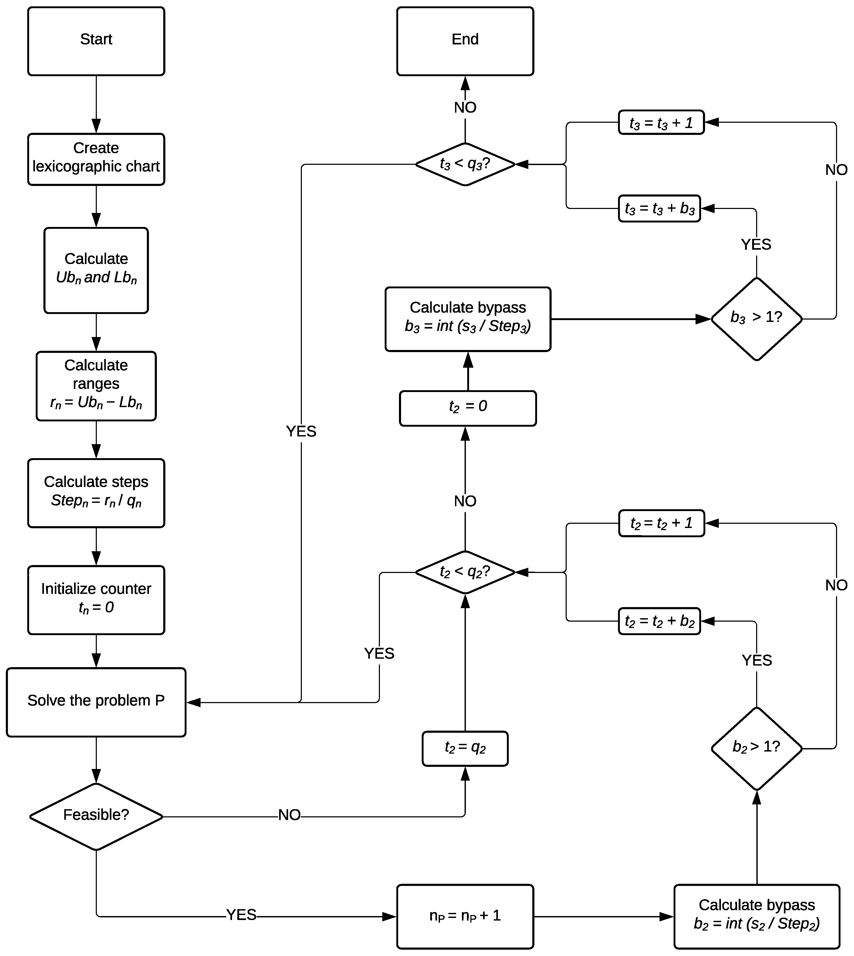
The AUG2 method creates a lexicographic chart that minimizes objectives F 1 , F 2 , and F 3 without restrictions. These minimized values are then used to calculate the upper ( U b n ) and lower ( L b n ) bounds for each objective F n . Following this, the range r n = U b n L b n is determined, which helps establish the size of the iteration step, S t e p n = r n / q n , where q n is a predefined number of points. The iteration begins with t n = 0 , and during each iteration, the value is updated using e n = U b n t n S t e p n . If a feasible solution is found, it is stored, and the bypass coefficient b n is computed to potentially skip subsequent iterations if the surplus ( s n ) exceeds S t e p n . The algorithm concludes if no feasible solution is identified (see Figure 2).
The following section describes the application of the Kernel search matheuristic algorithm and its MOSCLSCN application. The Kernel search matheuristic is applied at each iteration of the AUG2 method, yielding the Pareto front solution to the problem.

2.4.2. Kernel Search Matheuristic Application (KS)

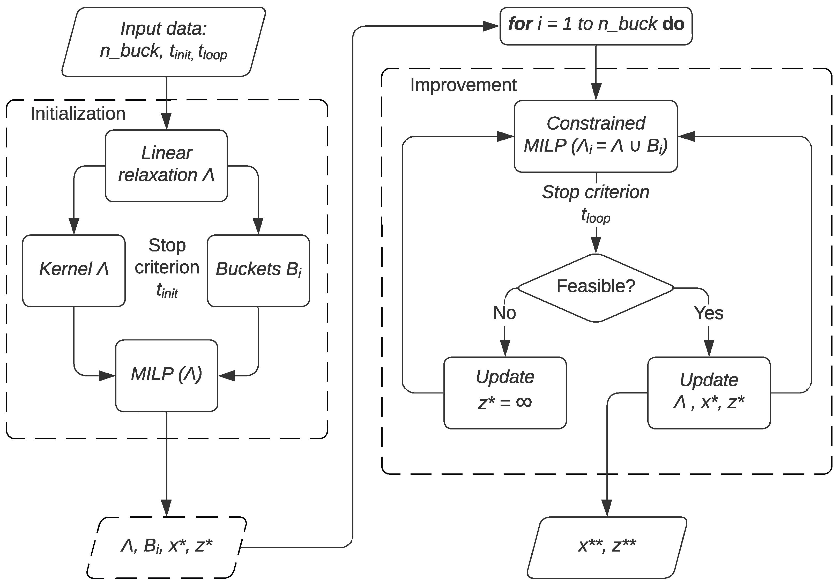
The Kernel search matheuristic is a two-phase framework that divides the main problem into sub-problems to be solved efficiently, including the initialization and improvement phases (see Figure 3). The Kernel search algorithm is a matheuristic documented in the book by Maniezzo et al. [4], which clearly explains its application to solve problems with binary variables, as demonstrated in Zhang et al. [37], Filippi et al. [38], Archetti et al. [39], Borčinová [40], Zhang et al. [41]. In our work, we implemented the Kernel search for non-binary variables.
The input parameters t i n i t _ t l o o p , and n _ b u c k are stated to be initialized. The initialization phase starts with the linear relaxation, with time t i n i t applied to obtain the promising variables ( x > 0 ), Kernel Λ , and the remaining variables are sorted by decreasing reduced cost and divided into n _ b u c k as B i . Then, the MILP is solved using ( Λ ) to obtain the solution x and its corresponding cost z . The improvement phase applies a heuristic that loops the constrained MILP, adding the constraints j B i x j 1 , which encourages the use of a variable from B i , a cutoff constraint z < z , and a time limit t l o o p . If the solution is feasible, it updates the Kernel Λ , the solution x , and its cost z . If not, the cost z = , so the process can continue. Finally, the algorithm reports the best solution, x , and its corresponding cost, z .

2.4.3. KS-MOSCLSCN Adaptation

The Kernel search matheuristic adaptations are applied to the payoff matrix in each iteration of the MOSCLSCN problem. In the case of the lexicographic chart phase, where the objective functions are solved independently (see Figure 2), the objective function F 2 (2) requires the application of Kernel search because of its quantity variable of vehicles, after this, in each iteration of the AUG2 framework. The Kernel search matheuristic requires the following procedure (see Algorithm 1). In the initialization phase, the linear relaxation is applied by changing the domain’s integer vehicles utilized variables ( V m w t v k , V w c t v k , V m h t v k , V h c t v k , V c h t v k , V h m t v k ) of the Equation (35) into continuous variables and solving the MOSCLSCN objective (38) with a time limit t i n i t . The obtained non-negative variables are sorted in decreasing order of reduced cost to define the Kernel set, and the remaining variables are considered buckets. The buckets are divided into n _ b u c k groups to obtain B i . After that, we solve the MOMILP with the Kernel Λ , resulting in the solution x , where the vehicle’s value-utilized variables are stored, and its F 2 value is stored at z . Then, in the improvement phase, the constrained MILP (pushed to use a variable from bucket B i with the constraint j B i x j 1 and cutting off constraint z < z ) is executed in a loop to explore the buckets obtained, updating the Λ that is selected in x in each iteration.
Algorithm 1 Kernel search matheuristic MOSCLSCN
1:  Input: n _ b u c k , t i n i t , t l o o p Output: x , z
2:  Let F = MOMILP formulation, where the vector x storage the values of V t v k variables, and z the value of F 2 ;
3: Solve LP-Relaxation of F with a time limit t i n i t
4:  Sort the variables x results by decreasing reduced costs;
5: Build the initial kernel Λ and a sequence of n _ b u c k buckets from x obtained;
6: Solve F ( Λ ) with a time limit t i n i t , let x and z be the best solution and its cost;
7: for  i = 1 to n _ b u c k do
8:      Construct the set Λ i = Λ B i ;
9:      Add to F ( Λ i ) the constraint j B i x j 1 ;
10:    Add to F ( Λ i ) the constraint z < z ;
11:    Solve F ( Λ i ) with time limit t l o o p
12:    if feasible solution found then
13:         Let x and z be the best solution and its cost;
14:         Add to Λ the variables which belong to B i and have been selected in x ;
15:     end if
16:     if no feasible solution found then
17:         Let z =
18:     end if
19: end for
20: Let x , z be the best solution from the storage solutions x , z .

2.5. Computational Experiment

In this section, we implement the solution methods and analyze their performance based on the obtained Pareto fronts. For clarity, we use acronyms for the approaches: the model with the AUG2 method is denoted INT, and the Kernel search matheuristic is denoted KS. The solution approaches were coded and implemented in Python 3.11.7 (packaged by Anaconda, Inc., Austin, TX, USA) in JupyterLab Version 4.0.11, and the solutions were generated using Gurobi Optimizer version 11.0.3. The equipment used was a PC with a 13th Gen Intel(R) Core(TM) i9-13900 2.00 GHz processor and 32 GB of RAM, running Windows 11 Pro. A maximum time limit of 7200 s per iteration was set for all experimentation unless otherwise stated.

2.5.1. Dataset Characteristics

To conduct experiments with the MOSCLSCN model using the Kernel search matheuristic, we generate a dataset based on the network characteristics described in Pazhani et al. [43] and Rodríguez-Escoto et al. [32]. To ensure consistency and comparability with the benchmark experiments on which our work is based, we configured a set of 14 instances by replicating the instance generation process. This set includes instances of varying sizes (different numbers of potential facility locations, customers, products, and/or periods) to systematically evaluate the scalability and behavior of the proposed solution method across different problem scales. Table 4 presents the network parameters for each instance, arranged from left to right. The parameters include the random number ( s e e d ), the number of suppliers (S), manufacturers (M), warehouses (W), hybrid facilities (H), retailers (C), products (P), raw materials (I), periods (T), type (V) and size (K) of vehicle, urban centers (U), number of nodes ( # N ), and the number of paths ( # P ) of the network. The datasets ofor this proposed study will be available at https://github.com/EliasOBoptlog/KS_MOSCLSCN (accessed on 7 February 2026).

2.5.2. Performance Metrics

To assess the effectiveness of the Kernel search algorithm employed for the MOSCLSCN problem, we will examine several factors: non-dominated solutions (NPS), computational time (CPU time), and distribution and spacing metrics of the resulting Pareto front. Regarding the latter, we will focus on the mean ideal distance (MID), the spacing metric (SM), and the hypervolume indicator (HV) [44,45]. Additionally, to standardize the terminology of the performance metrics, where i = 1 P a r e t o f r o n t and j = 1 S o l u t i o n s , we present the following terminology:
P F C = Non-dominated   combined Pareto front
P F i = Non-dominated   evaluated Pareto front   i
y x = The solution   x   i s   d o m i n a t e d   b y   t h e   s o l u t i o n   y
S j = A solution j   o f   t h e   P a r e t o   f r o n t
RPOS
The ratio of Pareto-optimal solutions is computed between the non-dominated evaluated Pareto obtained front from the non-dominated combined Pareto front and the original non-dominated evaluated Pareto front. A higher ratio is preferable, as it indicates better performance [46].
R P O S ( P F i ) = | P F i x P F i | y P F C : y x | | P F i |
QM
This quality metric evaluates the relationship between the evaluated non-dominated Pareto front and the combined non-dominated Pareto fronts. A higher value of this ratio is considered more favorable [47].
Q M ( P F i ) = | P F i x P F i | y P F C : y x | | P F C |
MID
The mean ideal distance measures the average Euclidean distance between a solution of the Pareto front and the ideal point in the objective space. The smaller the value, the better.
M I D ( P F i ) = j = 1 n S j B e s t S j M a x S j M i n S j 2 n
SM
The spacing metric assesses the distribution of Pareto-optimal solutions in the objective space by calculating the average difference between the Euclidean distance d j of adjacent solutions and the mean Euclidean distance d ¯ . A lower value indicates a better distribution of solutions.
S M ( P F i ) = j = 1 n 1 d j d ¯ ( n 1 ) d ¯
HV
The hypervolume indicator measures the volume of the objective space covered by the Pareto front P F i , bounded by a reference point r = m a x ( F i ) R m . It is defined so that for every point y P F i , we have y r , where β m indicates the Lebesgue m-dimensional measure (with m = 3 ). Normalizing the hypervolume value by the cube’s volume facilitates comparing HV values across different HV ranges. A higher value is preferred.
H V ( P F i ; r ) = β m y P F i y , r

2.5.3. Parameter Tuning

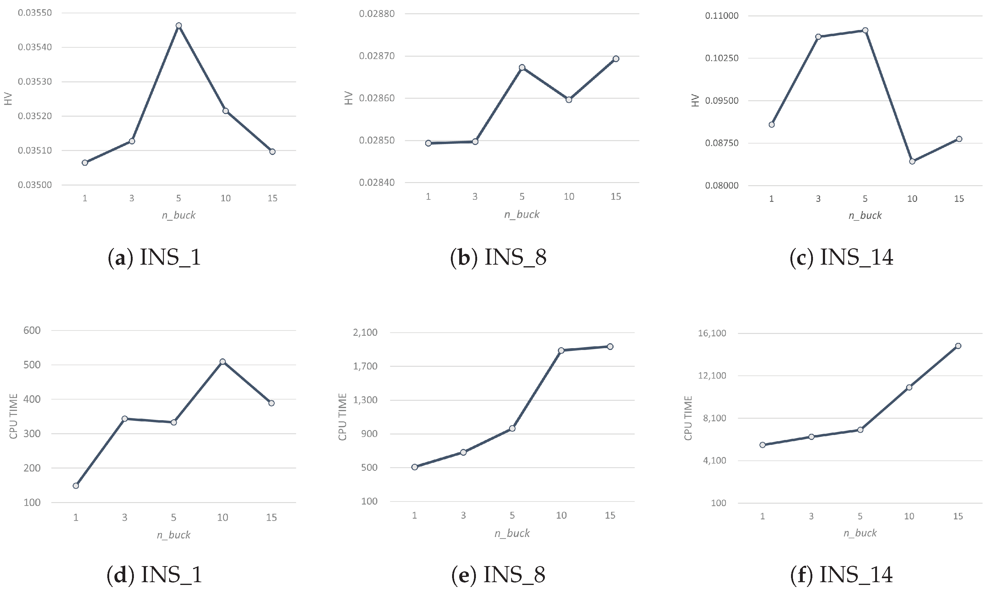
The parameter inputs needed to apply the Kernel search matheuristic are the number of buckets n _ b u c k and the time limits t i m e ( t i n i t _ t l o o p ). According to the Kernel search matheuristic works found, the way they stated the parameters was ad hoc to the instance size or context problem, and their preliminary experiment. For example, Archetti et al. [39] reported 10 buckets, Borčinová [40] explored from of 2 to 11 buckets, and Zhang et al. [41] reported 2 and 3 buckets. We have explored 1, 3, 5, 10, and 15 buckets.
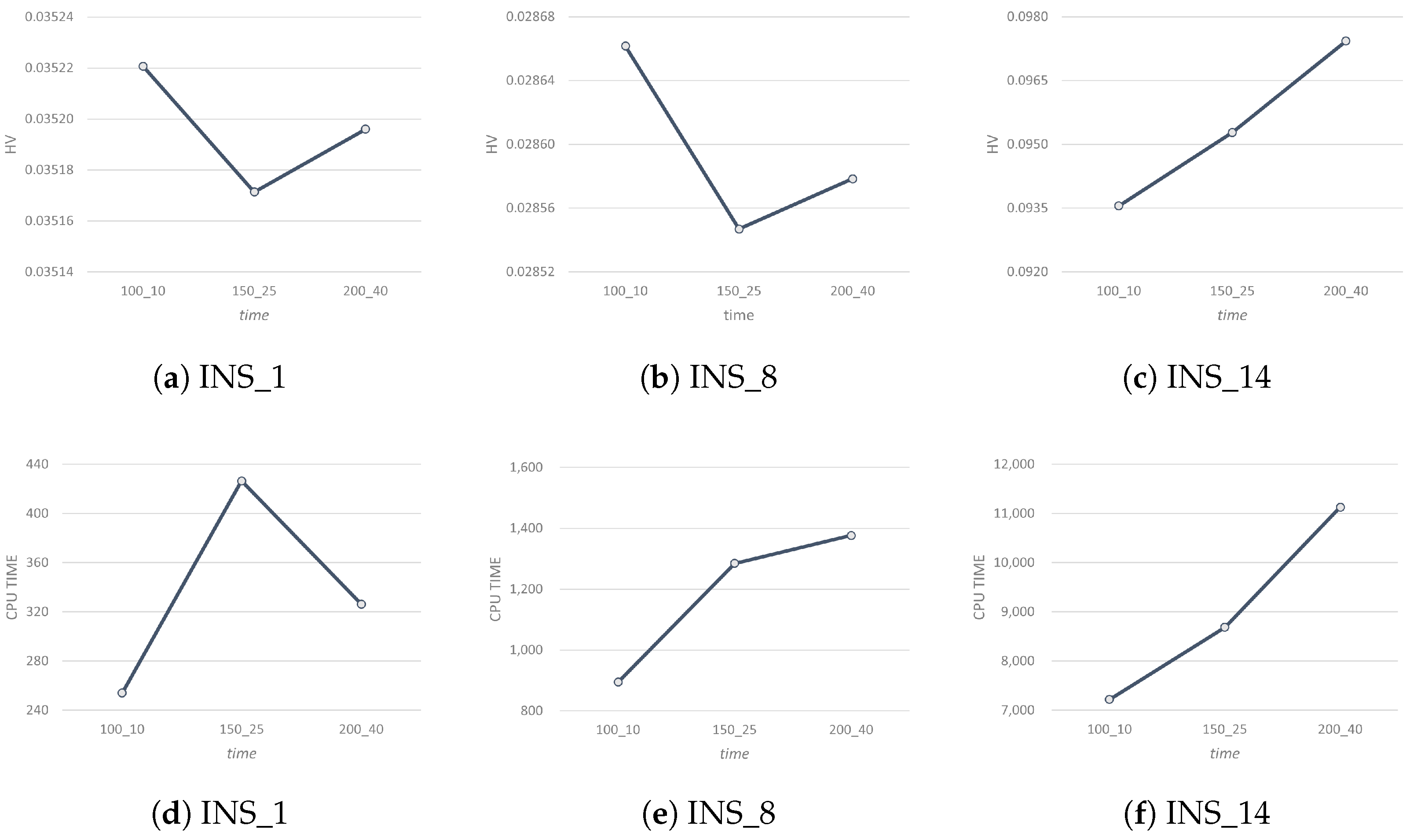
After observing the number of iterations of the INT method, we divided the 7200 s limit by 50 iterations, obtaining an approximate time of 150 s. We stated 150_25 s as parameter time ( t i n i t _ t l o o p ). To explore other parameters of time, 200_40 and 100_10 s were used. These parameters were tested with three representative sizes of instances: a small (INS_1), a medium (INS_8), and a large (INS_14). The hypervolume indicator was used to select values because its scalar value represents the quality of the Pareto front obtained and the CPU time, with the lowest value being the most desirable.
Figure 4a–c illustrate the HV performance, and Figure 4d–f illustrate the CPU time outcomes for each of the three instance sizes and numbers of buckets. The 5-bucket instance shows a higher HV and reports medium CPU time results compared to the other numbers of buckets.
Figure 5a–c illustrates the HV performance, and Figure 5d–f illustrates the CPU time outcomes in each parameter time. We can observe higher HV values in 100_10 for the small and medium instances, whereas the best performance was achieved with the 200_40 time configuration for the large instance. The experimentation was subsequently performed with n b u c k = 5 . For the parameter time, 100_10 was used for INS_1 to INS_8 and 200_40 for INS_9 to INS_14. The latter parameter is consistent with the number of paths # P of the instances. Instances 1 to 8 explore 3750 to 90,000 possible paths, while instances 9 to 14 explore 180,000 to 123,7500 possible paths. The selection of the time parameter is justified, due to the two-fold possible number of paths in INS_9. The HV indicators were calculated by comparing the Pareto fronts of the INT and KS applications.

3. Results and Discussion

The performance of the Kernel search matheuristic was compared to the results of the AUG2 method (INT). Performance metrics compared the Pareto fronts combined in QM, RPOS, and HV. The MID and SM metrics were evaluated independently.
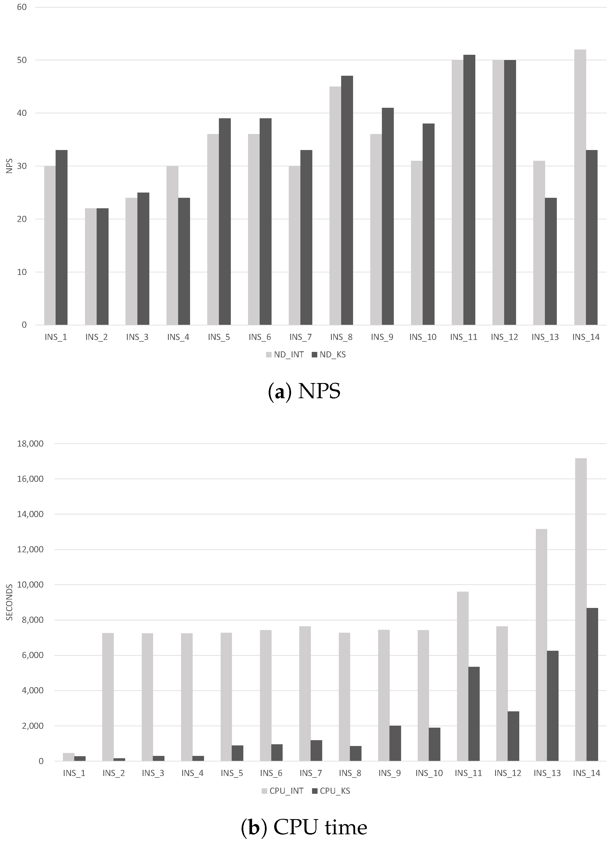
Table 5 displays the combined non-dominated solutions per method and the CPU time per instance. On average, the KS matheuristic improved the AUG2 method by 72% in CPU time while obtaining the same quantity of non-dominated solutions.
Table 6 displays the results of performance metrics per method. On average, the KS matheuristic improved the QM by 28.18%, the RPOS by 27.70%, the MID by 1.24%, the SM by 0.47%, and the HV by 2.15%.
The NPS results per method (see Figure 6a) indicate a good performance regarding both algorithms. Notably, we observed that KS obtained 64.3% more solutions, INT obtained 21.4% of total instances, and 14.3% were tied (see Table 5). According to the CPU time (see Figure 6b), the KS matheuristic outperforms the INT method in each instance.

4. Conclusions

In this paper, we propose a Kernel search (KS) matheuristic to address a multi-objective sustainable closed-loop supply chain network (MOSCLSCN) design problem. The model incorporates key decisions on facility location, inventory management, flow assignment, integration of forward and reverse logistics, and sustainability across economic, environmental, and social dimensions. Given that the underlying problem is NP-hard, its inherent complexity necessitates the development of efficient approximate solution methods.
The Kernel search matheuristic, introduced initially for binary decision problems, has been predominantly applied in that context. In this study, we extend its framework to handle binary and integer variables, thereby demonstrating its versatility across mixed-integer linear programming (MILP) settings. To the best of our knowledge, this is the first application of the KS matheuristic to a multi-objective sustainable closed-loop supply chain network design problem.
Computational experiments were conducted on 14 problem instances, with Pareto-optimal fronts generated using input parameters derived from a systematic experimental design. Although the tested instances provide a robust basis for performance evaluation and benchmarking against prior studies, larger-scale instances could further assess the method’s scalability. However, consultations with industry practitioners indicate that the largest instances examined here already reflect realistic problem sizes encountered in practical closed-loop supply chain network design. Practitioners note that huge instances often exceed typical operational scales, where computational time, data availability, and decision-making horizons impose practical limits. Consequently, further increases in size may offer diminishing returns in terms of real-world relevance. Nevertheless, the proposed KS matheuristic exhibits strong performance at the tested scales and scales efficiently to moderately larger problems if required.
We compared the KS matheuristic against the incumbent INT method using standard performance metrics. The results show that KS consistently outperforms INT, achieving an average computational time reduction of 72% while improving the solution quality metrics by 0.47% to 28.18%.
Practical decision-making often requires rapid evaluation of multiple parameter settings, sensitivity analyses, or adaptive re-optimization in response to dynamic conditions (e.g., demand variability, cost changes, or input uncertainty). Exact methods, despite guaranteeing optimality, frequently entail prohibitive runtimes, rendering them unsuitable for iterative or time-critical applications. This limitation underscores the value of effective matheuristics that deliver high-quality (near-optimal) solutions within practically acceptable computational times, thereby supporting rapid what-if analyses, interactive decision support, and timely operational deployment.
Building on these performance gains, future research directions include applying the KS matheuristic within alternative multi-objective scalarization frameworks, such as the weighted-sum, T-Chebyshev, and goal-programming methods. The MOSCLSCN model can also be extended to incorporate additional decisions or features (e.g., extra echelons, alternative transportation modes, advanced facility technologies, stricter carbon policies, or explicit uncertainty scenarios). Such extensions naturally increase the model size (in terms of variables and constraints), solver effort, and memory requirements. As a multi-objective MILP embedding NP-hard facility location decisions and multi-period integer flows, the formulation inherits the computational challenges typical of large-scale MILPs, further justifying the adoption of a matheuristic approach.
Although adapting the KS framework is non-trivial—particularly with respect to handling additional variable types (e.g., location and flow variables), bucket partitioning, and execution time calibration—promising avenues could include extending it to stochastic or dynamic environments. Relevant developments could encompass expected-value optimization, conditional value-at-risk (CVaR) for risk aversion, and robust optimization to explicitly address uncertainty in demand, costs, lead times, and other parameters.

Author Contributions

Conceptualization, J.-N.R.-E. and E.O.-B.; methodology, J.-N.R.-E.; software, J.-N.R.-E.; validation, E.O.-B., S.N.-G. and J.D.; formal analysis, E.O.-B. and J.D.; investigation, J.-N.R.-E.; data curation, J.-N.R.-E.; writing—original draft preparation, J.-N.R.-E.; writing—review and editing, E.O.-B., S.N.-G. and J.D.; supervision, E.O.-B.; funding acquisition, J.-N.R.-E.; project administration, E.O.-B. and S.N.-G.; resources, S.N.-G.; visualization, J.-N.R.-E. All authors have read and agreed to the published version of the manuscript.

Funding

This research was funded by Universidad Panamericana (grant number UP-GDL-22031104-50002-0175945).

Data Availability Statement

The data presented in this study are openly available in GitHub at https://github.com/EliasOBoptlog/KS_MOSCLSCN (accessed on 7 February 2026).

Conflicts of Interest

The authors declare no conflicts of interest.

References

  1. Barbosa-Póvoa, A.P.; da Silva, C.; Carvalho, A. Opportunities and challenges in sustainable supply chain: An operations research perspective. Eur. J. Oper. Res. 2018, 268, 399–431. [Google Scholar] [CrossRef]
  2. Tavana, M.; Kian, H.; Nasr, A.K.; Govindan, K.; Mina, H. A comprehensive framework for sustainable closed-loop supply chain network design. J. Clean. Prod. 2022, 332, 129777. [Google Scholar] [CrossRef]
  3. Govindan, K.; Soleimani, H.; Kannan, D. Reverse logistics and closed-loop supply chain: A comprehensive review to explore the future. Eur. J. Oper. Res. 2015, 240, 603–626. [Google Scholar] [CrossRef]
  4. Maniezzo, V.; Boschetti, M.A.; Stützle, T. Matheuristics; Springer International Publishing: Cham, Switzerland, 2021. [Google Scholar] [CrossRef]
  5. Pazhani, S.; Ravindran, A.R. A bi-criteria model for closed loop supply chain network design. Int. J. Oper. Res. 2018, 31, 330–356. [Google Scholar] [CrossRef]
  6. Fleischmann, M.; Beullens, P.; Bloemhof-Ruwaard, J.M.; Wassenhove, L.N.V. The Impact of Product Recovery on Logistics Network Design. Prod. Oper. Manag. 2001, 10, 156–173. [Google Scholar] [CrossRef]
  7. Sarkis, J.; Dou, Y. Green Supply Chain Management: A Concise Introduction; Routledge: London, UK, 2017. [Google Scholar] [CrossRef]
  8. Joshi, S. A review on sustainable supply chain network design: Dimensions, paradigms, concepts, framework and future directions. Sustain. Oper. Comput. 2022, 3, 136–148. [Google Scholar] [CrossRef]
  9. Jayarathna, C.P.; Agdas, D.; Dawes, L.; Yigitcanlar, T. Multi-objective optimization for sustainable supply chain and logistics: A review. Sustainability 2021, 13, 13617. [Google Scholar] [CrossRef]
  10. Amin, S.H.; Zhang, G.; Eldali, M.N. A review of closed-loop supply chain models. J. Data Inf. Manag. 2020, 2, 279–307. [Google Scholar] [CrossRef]
  11. Krarup, J.; Pruzan, P.M. The simple plant location problem: Survey and synthesis. Eur. J. Oper. Res. 1983, 12, 36–81. [Google Scholar] [CrossRef]
  12. Cornuéjols, G.; Nemhauser, G.; Wolsey, L. The Uncapicitated Facility Location Problem; Technical Report; Cornell University Operations Research and Industrial Engineering: Ithaca, NY, USA, 1983. [Google Scholar]
  13. Soleimani, H.; Kannan, G. A hybrid particle swarm optimization and genetic algorithm for closed-loop supply chain network design in large-scale networks. Appl. Math. Model. 2015, 39, 3990–4012. [Google Scholar] [CrossRef]
  14. Hajiaghaei-Keshteli, M.; Fard, A.M.F. Sustainable closed-loop supply chain network design with discount supposition. Neural Comput. Appl. 2019, 31, 5343–5377. [Google Scholar] [CrossRef]
  15. Mehrjerdi, Y.Z.; Shafiee, M. Multiple-Sourcing in Sustainable Closed-loop Supply Chain Network Design: Tire Industry Case Study. Int. J. Supply Oper. Manag. 2020, 7, 202–221. [Google Scholar]
  16. Yun, Y.; Chuluunsukh, A.; Gen, M. Sustainable Closed-Loop Supply Chain Design Problem: A Hybrid Genetic Algorithm Approach. Mathematics 2020, 8, 84. [Google Scholar] [CrossRef]
  17. Khorshidvand, B.; Soleimnai, H.; Mehdi, M.; Esfahani, S.; Sibdari, S. Sustainable closed-loop supply chain network: Mathematical modeling and Lagrangian relaxation. J. Ind. Eng. Manag. Stud. 2021, 8, 240–260. [Google Scholar] [CrossRef]
  18. Pahlevan, S.M.; Hosseini, S.M.S.; Goli, A. Sustainable supply chain network design using products’ life cycle in the aluminum industry. Environ. Sci. Pollut. Res. 2021, 1–25. [Google Scholar] [CrossRef]
  19. Akbari-Kasgari, M.; Khademi-Zare, H.; Fakhrzad, B.M.; Hajiaghaei-Keshteli, M.; Honarvar, M. Designing a resilient and sustainable closed-loop supply chain network in copper industry. Clean Technol. Environ. Policy 2022, 24, 1553–1580. [Google Scholar] [CrossRef]
  20. Irawan, C.A.; Abdulrahman, M.D.A.; Salhi, S.; Luis, M. An efficient matheuristic algorithm for bi-objective sustainable closed-loop supply chain networks. IMA J. Manag. Math. 2022, 33, 603–636. [Google Scholar] [CrossRef]
  21. Mogale, D.G.; De, A.; Ghadge, A.; Aktas, E. Multi-objective modelling of sustainable closed-loop supply chain network with price-sensitive demand and consumer’s incentives. Comput. Ind. Eng. 2022, 168, 108105. [Google Scholar] [CrossRef]
  22. Seydanlou, P.; Jolai, F.; Tavakkoli-Moghaddam, R.; Fathollahi-Fard, A.M. A multi-objective optimization framework for a sustainable closed-loop supply chain network in the olive industry: Hybrid meta-heuristic algorithms. Expert Syst. Appl. 2022, 203, 117566. [Google Scholar] [CrossRef]
  23. Soleimani, H.; Chhetri, P.; Fathollahi-Fard, A.M.; Mirzapour Al-e-Hashem, S.M.J.; Shahparvari, S. Sustainable closed-loop supply chain with energy efficiency: Lagrangian relaxation, reformulations and heuristics. Ann. Oper. Res. 2022, 318, 531–556. [Google Scholar] [CrossRef]
  24. Tirkolaee, E.B.; Goli, A.; Ghasemi, P.; Goodarzian, F. Designing a sustainable closed-loop supply chain network of face masks during the COVID-19 pandemic: Pareto-based algorithms. J. Clean. Prod. 2022, 333, 130056. [Google Scholar] [CrossRef]
  25. Abbasi, S.; Daneshmand-Mehr, M.; Kanafi, A.G. Designing a Tri-Objective, Sustainable, Closed-Loop, and Multi-Echelon Supply Chain during the COVID-19 and Lockdowns. Found. Comput. Decis. Sci. 2023, 48, 269–312. [Google Scholar] [CrossRef]
  26. Becerra, P.; Mula, J.; Sanchis, R. Optimising location, inventory and transportation in a sustainable closed-loop supply chain. Int. J. Prod. Res. 2024, 62, 1609–1632. [Google Scholar] [CrossRef]
  27. Gholipour, A.; Sadegheih, A.; Mostafaeipour, A.; Fakhrzad, M.B. Designing an optimal multi-objective model for a sustainable closed-loop supply chain: A case study of pomegranate in Iran. Environ. Dev. Sustain. 2024, 26, 3993–4027. [Google Scholar] [CrossRef]
  28. Goodarzian, F.; Ghasemi, P.; Gonzalez, E.D.S.; Tirkolaee, E.B. A sustainable-circular citrus closed-loop supply chain configuration: Pareto-based algorithms. J. Environ. Manag. 2023, 328, 116892. [Google Scholar] [CrossRef] [PubMed]
  29. Mirzaei, M.G.; Goodarzian, F.; Mokhtari, K.; Yazdani, M.; Shokri, A. Designing a dual-channel closed loop supply chain network using advertising rate and price-dependent demand: Case study in tea industry. Expert Syst. Appl. 2023, 233, 120936. [Google Scholar] [CrossRef]
  30. Yamchi, H.R.; Jabarzadeh, Y.; Govindan, K.; Mahdiraji, H.A. A triple bottom line approach for designing a sustainable closed-loop supply chain network in fruit industry: A metaheuristic solution approach. J. Oper. Res. Soc. 2024, 75, 1925–1948. [Google Scholar] [CrossRef]
  31. Momeni, M.A.; Jain, V.; Bagheri, M. A Multi-Objective Model for Designing a Sustainable Closed-Loop Supply Chain Logistics Network. Logistics 2024, 8, 29. [Google Scholar] [CrossRef]
  32. Rodríguez-Escoto, J.N.; Olivares-Benitez, E.; Nucamendi-Guillén, S.; Drzymalski, J. A multi-objective sustainable closed-loop supply chain network problem with hybrid facilities. Int. Trans. Oper. Res. 2025, 32, 3497–3527. [Google Scholar] [CrossRef]
  33. Jebreili, S.; Babazadeh, R.; Fazayeli, S.; A. Kamran, M.; Gharibi, A.R. A Multi-Objective MILP Model for Sustainable Closed-Loop Supply Chain Network Design: Evidence from the Wood–Plastic Composite Industry. Mathematics 2025, 13, 3478. [Google Scholar] [CrossRef]
  34. Restrepo Diaz, J.D.; Amin, S.H. A multi-objective optimization approach for sustainable management of computers E-waste in a closed-loop supply chain network. J. Clean. Prod. 2025, 506, 145494. [Google Scholar] [CrossRef]
  35. Jauhari, W.A.; Wakhid, P.A. A multi-echelon closed-loop agricultural supply chain network problem for corn industry with waste recycling and carbon regulation. Model. Earth Syst. Environ. 2026, 12, 6. [Google Scholar] [CrossRef]
  36. Boschetti, M.A.; Maniezzo, V.; Roffilli, M.; Röhler, A.B. Matheuristics: Optimization, Simulation and Control. In Lecture Notes in Computer Science (Including Subseries Lecture Notes in Artificial Intelligence and Lecture Notes in Bioinformatics); Springer: Berlin/Heidelberg, Germany, 2009; Volume 5818 LNCS, pp. 171–177. [Google Scholar] [CrossRef]
  37. Zhang, Y.; Che, A.; Chu, F. Improved model and efficient method for bi-objective closed-loop food supply chain problem with returnable transport items. Int. J. Prod. Res. 2022, 60, 1051–1068. [Google Scholar] [CrossRef]
  38. Filippi, C.; Guastaroba, G.; Huerta-Muñoz, D.L.; Speranza, M.G. A kernel search heuristic for a fair facility location problem. Comput. Oper. Res. 2021, 132, 105292. [Google Scholar] [CrossRef]
  39. Archetti, C.; Guastaroba, G.; Huerta-Muñoz, D.L.; Speranza, M.G. A kernel search heuristic for the multivehicle inventory routing problem. Int. Trans. Oper. Res. 2021, 28, 2984–3013. [Google Scholar] [CrossRef]
  40. Borčinová, Z. Kernel Search for the Capacitated Vehicle Routing Problem. Appl. Sci. 2022, 12, 11421. [Google Scholar] [CrossRef]
  41. Zhang, Y.; Chu, F.; Che, A.; Li, Y. Closed-loop inventory routing problem for perishable food with returnable transport items selection. Int. J. Prod. Res. 2024, 62, 501–521. [Google Scholar] [CrossRef]
  42. Mavrotas, G.; Florios, K. An improved version of the augmented ϵ-constraint method (AUGMECON2) for finding the exact pareto set in multi-objective integer programming problems. Appl. Math. Comput. 2013, 219, 9652–9669. [Google Scholar] [CrossRef]
  43. Pazhani, S.; Mendoza, A.; Nambirajan, R.; Narendran, T.T.; Ganesh, K.; Olivares-Benitez, E. Multi-period multi-product closed loop supply chain network design: A relaxation approach. Comput. Ind. Eng. 2021, 155, 107191. [Google Scholar] [CrossRef]
  44. Zitzler, E.; Thiele, L.; Laumanns, M.; Fonseca, C.M.; Fonseca, V.G.D. Performance assessment of multiobjective optimizers: An analysis and review. IEEE Trans. Evol. Comput. 2003, 7, 117–132. [Google Scholar] [CrossRef]
  45. Audet, C.; Bigeon, J.; Cartier, D.; Digabel, S.L.; Salomon, L. Performance indicators in multiobjective optimization. Eur. J. Oper. Res. 2021, 292, 397–422. [Google Scholar] [CrossRef]
  46. Altiparmak, F.; Gen, M.; Lin, L.; Paksoy, T. A genetic algorithm approach for multi-objective optimization of supply chain networks. Comput. Ind. Eng. 2006, 51, 196–215. [Google Scholar] [CrossRef]
  47. Rayat, F.; Musavi, M.; Bozorgi-Amiri, A. Bi-objective reliable location-inventory-routing problem with partial backordering under disruption risks: A modified AMOSA approach. Appl. Soft Comput. 2017, 59, 622–643. [Google Scholar] [CrossRef]
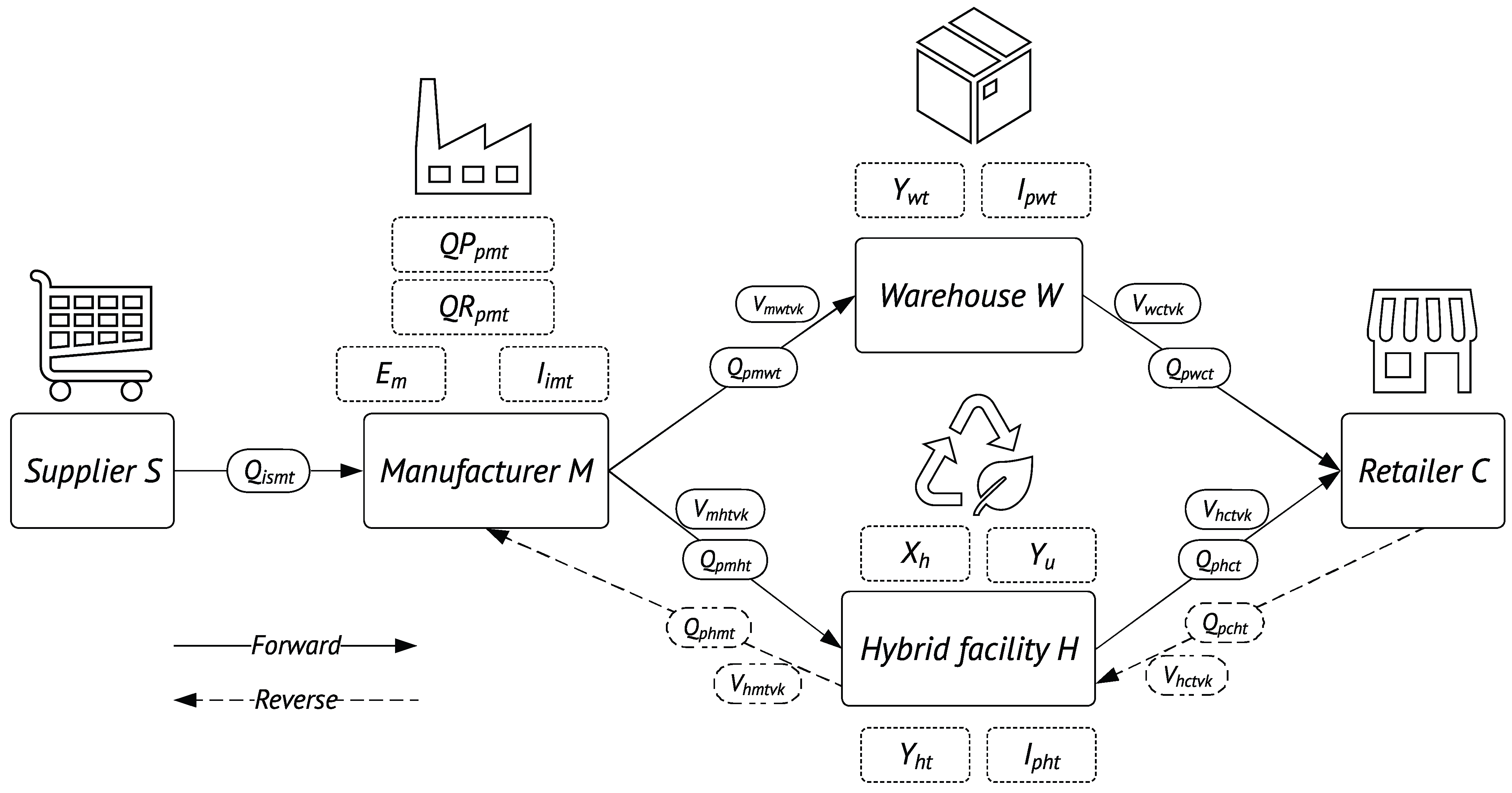
Figure 1. SCLSCN network.
Mathematics 14 00773 g001
Figure 2. AUG2 method diagram.
Mathematics 14 00773 g002
Figure 3. Kernel search matheuristic.
Mathematics 14 00773 g003
Figure 4. HV performance and CPU time through n b u c k parameters.
Mathematics 14 00773 g004
Figure 5. HV performance and CPU time through time parameters.
Mathematics 14 00773 g005
Figure 6. NPS and CPU time of Pareto fronts.
Mathematics 14 00773 g006
Table 2. Parameters of the model.
NotationDescription
I C i m Cost of inventory per unit of raw material i at manufacturer m
I C p w Cost of inventory per unit of product p at depot w
I C p h Cost of inventory per unit of product p at hybrid facility h
C R M i s m Cost per unit of raw material i when supplied by s to m
T C m w Cost of transport per unit weight from manufacturer m to depot w
T C m h Cost of transport per unit weight from manufacturer m to hybrid facility h
T C w c Cost of transport per unit weight from depot w to retailer c
T C h c Cost of transport per unit weight from hybrid facility h to retailer c
T C c h Cost of transport per unit weight from retailer c to hybrid facility h
T C h m Cost of transport per unit weight from hybrid facility h to manufacturer m
P C p m The production expense of product p at manufacturer m
R C p m The recycling expense of product p in manufacturer m
D p c t Retailer demand c for product p in time period t
F C w Opening cost for warehouse w
F C h Opening cost for hybrid facility h
F C m Opening cost for manufacturer m
S C w Capacity for storage at depot w
S C h Capacity for storage in hybrid facility h
S C m Capacity for storage at manufacturer m
M C m Manufacturing capacity limit per manufacturer m
W p Weight of product p
B p Disposal rate of product p
O F F i p Offtake of raw material i for product p
A p c t Return rate of product p available in retailer c at time period t
S L Service level
S D S p Sales standard deviation of product p
L p Average lead time for product p at retailers
M B Big number
eNumber near to 1
V C v k Vehicle cost of type v and size k
V Q v k Vehicle capacity of type v and size k
C O v k CO2 emissions of vehicle v and size k
P O P u The urban center population u
D I S u h Distance between urban centers u to hybrid facilities h
S U R A zone of negative influence surrounding a facility
Table 3. Variables of the model.
NotationDescription
Q i s m t Raw material i quantity acquired from supplier s by manufacturer m in time period t
Q P p m t Product p quantity produced by manufacturer m in time period t
Q R p m t Product p quantity recycled at manufacturing plant m in time period t
Q p m w t Product p quantity shipped from manufacturer m to depot w in time period t
Q p m h t Product p quantity shipped from manufacturer m to hybrid facility h in time period t
Q p w c t Product p quantity shipped from depot w to retailer c in time period t
Q p h c t Product p quantity shipped from hybrid facility h to retailer c in time period t
Q p c h t Product p quantity shipped from retailer c to hybrid facility h in time period t
Q p h m t Product p quantity shipped from hybrid facility h to manufacturer m in time period t
D Q p h m t An auxiliary variable for Q p h m t
I i m t Raw material inventory i is available at manufacturer m in time period t
I p w t Product inventory p is available in depot w in time period t
I p h t Product inventory p is available at hybrid facility h in time period t
V m w t v k Vehicles chosen for transportation between manufacturer m and warehouse w
V w c t v k Vehicles chosen for transportation between warehouse w to retailer c
V m h t v k Vehicles chosen for transportation between manufacturer m to hybrid facility h
V h c t v k Vehicles chosen for transportation between hybrid facility h to retailer c
V c h t v k Vehicles chosen for transportation between retailer c to hybrid facility h
V h m t v k Vehicles chosen for transportation between hybrid facility h to manufacturer m
Y w t 1 if warehouse w is active during time period t, and 0 if it is inactive.
Y h t 1 if hybrid facility h is active during time period t, and 0 if it is inactive.
E m 1 if manufacturer m is opened, and 0 if it is inactive.
X h 1 if hybrid facility h is closed and unoccupied, and 0 if site h is operational.
Y u 1 if urban center u is within the negative impact zone of any hybrid facility, and 0 if it is outside.
S E L Hybrid facility opened
Table 4. Dataset characteristics.
Parameters Seed SMWHCPITVKU # N # P
INS_11535510335236283750
INS_22535510335236283750
INS_33835515345236369000
INS_44835515345236369000
INS_55103105253552365337,500
INS_66103105253552365337,500
INS_772031053031052366890,000
INS_882031053031052366890,000
INS_9910315104035523678180,000
INS_101010315104035523678180,000
INS_1111203151045310523693405,000
INS_1212203151045310523693405,000
INS_13132031812503105236103648,000
INS_141425320155531552361181,237,500
Table 5. NPS and CPU time of INT and KS.
InstanceND CombinedND_INTND_KSCPU_INTCPU_KS
INS_1462128455280
INS_23818247259162
INS_33722157250297
INS_44324237248295
INS_55720377281891
INS_66427377427956
INS_750252776391182
INS_87431467286850
INS_957293174422001
INS_1053312574221895
INS_1170244696045339
INS_1275275076332821
INS_1334112313,1546250
INS_1453273317,1668689
Average53.6424.0731.7981622279
Table 6. Performance metrics of INT and KS.
InstanceQMRPOSMIDSMHV
INTKSINTKSINTKSINTKSINTKS
INS_10.4570.6090.7000.8491.0090.9991.8581.8700.0350.035
INS_20.4740.6320.8181.0911.0050.9431.8091.8080.0540.055
INS_30.5950.4050.9170.6001.0380.9901.7381.7490.1480.149
INS_40.5580.5350.8000.9580.8890.8851.8611.8320.1190.122
INS_50.3510.6490.5560.9491.1171.0781.7701.7880.0500.050
INS_60.4220.5780.7500.9491.0951.0571.8271.8390.0370.037
INS_70.5000.5400.8330.8180.9991.0191.8131.8250.0790.079
INS_80.4190.6220.6890.9791.0151.0061.8161.8210.0290.029
INS_90.5090.5440.8060.7560.9830.9941.8251.8460.0420.042
INS_100.5850.4721.0000.6581.0871.0841.7991.8360.0460.047
INS_110.3430.6570.4800.9020.9120.9181.7941.7770.0760.077
INS_120.3600.6670.5401.0000.9090.9111.7951.7940.1450.145
INS_130.3240.6770.3550.9581.2061.2121.7981.7360.0150.016
INS_140.5090.6230.5191.0001.0751.0691.7621.6220.0970.110
Average0.4570.5860.6970.8911.0241.0121.8051.7960.0690.071
Disclaimer/Publisher’s Note: The statements, opinions and data contained in all publications are solely those of the individual author(s) and contributor(s) and not of MDPI and/or the editor(s). MDPI and/or the editor(s) disclaim responsibility for any injury to people or property resulting from any ideas, methods, instructions or products referred to in the content.