Residual Low-Order Phase-Error Estimation and Compensation for Post-Autofocus UAV K-Band Multi-Baseline InSAR

Abstract

This study examines residual low-order (linear and constant) phase errors in interferometric synthetic aperture radar (InSAR) when compact, high-frequency radar sensors are mounted on commercial uncrewed aerial vehicles (UAVs). Although higher carrier frequencies and shorter standoff ranges enable fine-resolution interferometry, the same characteristics—together with UAV platform instability—make the system highly vulnerable to motion-induced phase errors, which can significantly degrade or even invalidate DEM reconstruction. This paper first quantifies the admissible motion-error bounds for reliable multi-baseline phase-gradient estimation, and then introduces a post-autofocus correction scheme that estimates the residual linear term from the interferometric fringe frequency and refines it via an FFT-based correlation objective, while the constant term is calibrated using ground control points (GCPs). The method is validated through simulations of a 24 GHz UAV demonstrator. To the best of our knowledge, this work provides the first post-autofocus demonstration of linear-and-constant residual-error mitigation for UAV-based high-frequency multi-baseline InSAR. In the considered K-band setting, the proposed approach reduces the DEM error from 42 m to 0.2 m (≈98% improvement).

1. Introduction

Interferometric synthetic aperture radar (InSAR) is a key three-dimensional remote-sensing technique for generating high-precision digital elevation models (DEMs), supporting applications such as accurate mapping, rapid post-disaster assessment, and emergency terrain monitoring [1,2,3,4,5,6]. To further improve elevation accuracy, multi-baseline InSAR is widely adopted. A number of studies have analyzed multi-baseline phase-gradient estimation from probabilistic and mathematical viewpoints [7,8,9,10]. Because phase gradients must be inferred between neighboring pixels, even small residual phase errors can corrupt the gradient estimates and, in turn, cause severe DEM reconstruction failures.

Most SAR/InSAR systems have traditionally relied on satellite or manned airborne platforms. In recent years, uncrewed aerial vehicles (UAVs) have become an attractive alternative thanks to their low cost, portability, rapid deployment, and ability to operate in hazardous or hard-to-reach areas. UAV-borne SAR has been reported across a broad frequency range, from P-band medium-resolution systems to W-band ultra-high-resolution implementations [11,12,13,14,15,16,17]. The multi-baseline system considered here operates at K-band, where high-resolution interferometry can be achieved with a compact antenna, helping to meet UAV payload constraints. Compared with lower-frequency InSAR, K-band is more sensitive to atmospheric effects; however, the short-range configuration used in this study limits such impacts. At the same time, near-range K-band InSAR becomes more sensitive to geometric-model inaccuracies—particularly residual low-order motion errors—which propagate directly into elevation estimates and thus degrade DEM accuracy.

In our configuration, motion-induced phase errors are spatially variant, so interferogram-domain compensation methods designed for spatially invariant errors (e.g., [18,19]) are not directly applicable. This paper therefore adopts a motion-compensation strategy that forms repeat-pass interferometric baselines and enhances image coherence via trajectory-dependent autofocus for each flight [20,21]. Nevertheless, the autofocus techniques used in practice [22,23,24,25] cannot remove all motion effects, leaving residual linear and constant components that may critically impair multi-baseline processing. For the geometry studied here (≈100 m altitude and ≈45° incidence within the synthetic aperture), the higher-order terms and constant components discussed in [22] are typically much smaller than the residual linear component and can be neglected relative to it.

The UAV experiments in this work are configured with a flight altitude of approximately 100 m, and the imaged area is centered near an incidence angle of about 45°. Under these conditions, the spatial variation of the residual linear term can be treated as weak. Existing UAV-InSAR research has mainly focused on geometric modeling, imaging, and baseline design, whereas fewer studies have quantitatively linked residual motion errors to multi-baseline phase-gradient reliability and DEM accuracy. For example, refs. [18,26] reported decimeter-level DEM errors at L-band. At lower frequencies, the coarser resolution may obscure fine target details. In a comparable high-frequency setting, ref. [27] achieved notable results, but the reported DEM error is around 1 m. Related repeat-pass K-band residual phase compensation has also been investigated in [25,28]. Compared with those efforts, which primarily target coherence enhancement for coherent detection, the present work emphasizes improving elevation accuracy and multi-baseline phase-gradient robustness.

This study targets K-band UAV multi-baseline InSAR by starting from a physics-based trajectory model to explicitly expose the linear and constant components of post-autofocus residual motion errors in the interferometric phase. This paper derives an admissible error region for Chinese Remainder Theorem (CRT)-based phase-gradient estimation and proposes a two-stage mitigation strategy: estimating the linear phase term from interferometric fringes and compensating the constant phase bias using ground control points (GCPs). As a result, reliable decimeter-level DEM reconstruction becomes feasible on high-frequency UAV platforms, substantially improving the fault tolerance of multi-baseline InSAR to motion errors.

The proposed approach first infers the dominant linear-error frequency from the interferometric fringes. After estimating this frequency via the fast Fourier transform (FFT), a correlation-based objective is constructed to iteratively refine and compensate the linear phase term. The remaining constant phase bias is then removed using GCPs. Based on these steps, this paper presents a complete multi-baseline InSAR processing flow together with a dedicated residual-error compensation procedure. The theory is verified through simulations using a 24 GHz UAV radar demonstrator, this system was formed using 24 GHz INRAS radar, a DJI S900 UAV with an A3 flight controller and a Raspberry-Pi 3B microcontroller [24]. Section 2 introduces the multi-baseline geometry and quantifies how residual phase errors affect phase-gradient estimation, while Section 3 reports simulation results for an outdoor scene.

2. UAV-Based Multi-INSAR Concept

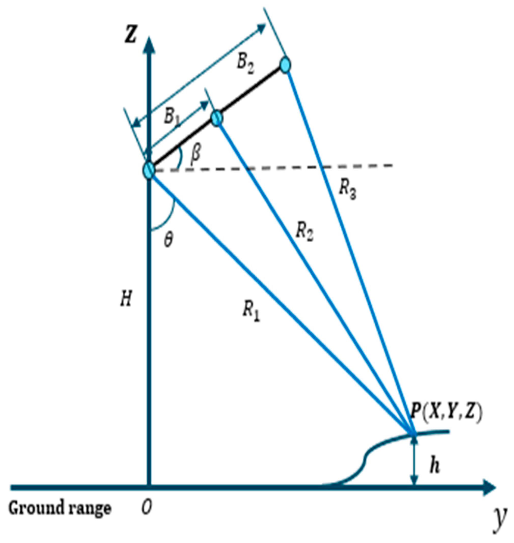
In repeat-pass mode, this paper describes multiple flights on the same platform to form multiple interferometric baselines. As shown in Figure 1, assume that there are two baselines, $B_1$ and $B_2$. The height h of the P pixel is calculated by the difference between $R_3$, $R_2$ and $R_1$ and the looking viewing angle $\theta$ of the main trajectory. $∆R$ is the interferometric range at point P, which is the difference between the slave slant range and the master slant range, where $∆R_{wrap}$ is the wrap phase, and $∆R_{am}$ is the ambiguity range. It will be elaborated on in detail below.

2.1. Residual-Error Decorrelation Source at Phase-Gradient Estimation

This paper considers multi-baseline InSAR in repeat-pass mode, where each trajectory is acquired independently. Statistically, every additional pass introduces an additional source of motion uncertainty. To quantify the resulting sensitivity, this paper adopts the phase-unwrapping error sensitivity metric in [20]:

$${\displaystyle \frac{{\sigma }_{h\left(s\right)}^{\psi \left(s\right)}}{{\sigma }_{\psi \left(s\right)}}}={\displaystyle \frac{\lambda R_{1}sin\theta }{4\pi }}\sqrt{{\displaystyle \frac{1}{{{B1}_{\perp }}^2}}+\cdots +{\displaystyle \frac{1}{{{Bn}_{\perp }}^2}}}$$

(1)

where ${\displaystyle \frac{{\sigma }_{h\left(s\right)}^{\psi \left(s\right)}}{{\sigma }_{\psi \left(s\right)}}}$ is the phase-unwrapping error sensitivity. $\lambda$ is the wavelength (0.0125 m). ${Bn}_{\perp }$ is the perpendicular baseline, which represents the vertical component of the n-th baseline in the triangular geometry with $R_1$. In Equation (1), the baseline is in the denominator, so increasing the baseline length will reduce the sensitivity of the phase error and reduce the impact of the error on the DEM. At the same time, increasing the number of baselines means adding a term related to the baseline in (1) and thus leads to sensitivity to phase-unwrapping errors and increases the impact of the error on the DEM. To mitigate the sources of motion error, two baselines were selected for testing. The selection of the baseline length is a multi-objective programming problem. A longer baseline will reduce the ambiguity height, increase the height sensitivity (high height accuracy), decrease the spatial decorrelation coefficient, and the residual error will have a greater impact on the DEM. A shorter baseline is the opposite, with a smaller impact of the residual error but lower height sensitivity [1,2]. This paper uses the solution in [20] to select the length of the baseline. The height of P is expressed in Figure 1 as follows [29]:

$$h\left(p\right)={\displaystyle \frac{\lambda }{4\pi }}{\displaystyle \frac{R_{1}sin\theta }{B_{n\perp }}}·{\psi }_n^{topo}\left(p\right)\hspace{1em}n = 1 \mathrm{or} 2$$

(2)

where ${{\psi }_n^{topo}\left(p\right)=\psi }_n^{all}(p)-{\psi }_n^{err}(p)$, and ${\psi }_n^{all}\left(p\right)$ is the flattened absolute interferometric phase (after phase unwrapping) of the Pth pixel in the n-th interferogram. ${\psi }_n^{topo}\left(p\right)$ is the topography height absolute n-th interferometric phase. ${\psi }_n^{err}\left(p\right)$ is the motion error absolute n-th interferometric phase.

Because the radar measures phase modulo 2π, it observes only the wrapped phase and cannot directly determine the number of 2π cycles. Accordingly, the pre-unwrapping phase can be written as [30]:

$${\phi }_n^{all}\left(p\right)={\psi }_n^{topo}\left(p\right)+{\psi }_n^{err}\left(p\right)-2\pi k_n\left(p\right)$$

(3)

where ${\phi }_n^{all}\left(p\right)$ is the wrapped phase measured by radar. $k_n\left(p\right)$ is the integer ambiguity number of the point P in the n-th interferogram. Ideally, the height of point P obtained from each baseline should be the same. By substituting $B_1$ and $B_1$ into (2) and then combining with (3), we can obtain [30]:

$$B_2\left[{\phi }_1^{all}\left(p\right)-{\psi }_1^{err}\left(p\right)-2\pi k_1\left(p\right)\right]=B_1\left[{\phi }_2^{all}\left(p\right)-{\psi }_2^{err}\left(p\right)-2\pi k_2\left(p\right)\right]$$

(4)

From a mathematical standpoint, let P denote a pixel index. If the relevant phase terms are continuous functions of P, the phase gradient corresponds to a first-order derivative along the direction S. For discrete imagery, the gradient is approximated by a first-order finite difference. Substituting P + 1 and P into (4) and subtracting the two expressions yields the phase-gradient relation:

$$B_2\left[{\phi }_1^{all}\left(p+1\right)-{\phi }_1^{all}\left(p\right)]-B_1[{\phi }_2^{all}\left(p+1\right)-{\phi }_2^{all}\left(p\right)]=B_2[{\psi }_1^{err}\left(p+1\right)-{\psi }_1^{err}\left(p\right)]-B_1[{\psi }_2^{err}\left(p+1\right)-{\psi }_2^{err}\left(p\right)]+2\pi (B_2\left[k_1\left(p+1\right)-k_1\left(p\right)\right]-B_1[k_2\left(p+1\right)-k_2\left(p\right)\right])$$

(5)

where:

$$\left\{\begin{array}{c}{∆{\phi }_n^{all}\left(p\right)=\phi }_n^{all}\left(p+1\right)-{\phi }_n^{all}\left(p\right)\\ {∆\psi }_n^{err}\left(p\right)={\psi }_n^{err}\left(p+1\right)-{\psi }_n^{err}\left(p\right)\\ ∆k_n\left(p\right)=k_n\left(p+1\right)-k_n\left(p\right)\end{array}\right.$$

(6)

In Equation (6), the phase gradient of system measurement $∆{\phi }_n^{all}\left(p\right)$, the phase-error gradient of motion ${∆\psi }_n^{err}\left(p\right)$ and the integer period (ambiguity number) gradient $∆k_n\left(p\right)$ are defined. By combining (5) and (6) and simplifying, it can be given by:

$$\left[{\displaystyle \frac{B_2}{B_1}}∆{\phi }_1^{all}\left(p\right)-∆{\phi }_2^{all}\left(p\right)\right]-∆\left(p\right)=2\pi k_{ture}\left(p\right)$$

(7)

$$k_{ture}\left(p\right)={\displaystyle \frac{B_2}{B_1}}∆k_1\left(p\right)-∆k_2\left(p\right)$$

(8)

$$∆\left(p\right)={\displaystyle \frac{B_2}{B_1}}{∆\psi }_1^{err}\left(p\right)-{∆\psi }_2^{err}\left(p\right)$$

(9)

Equation (7) is a congruence relation in the ambiguity numbers. Solving it gives the ambiguity numbers for the two baselines, as summarized in (8). Equation (9) further quantifies how motion errors perturb this congruence. This paper employs the Two-Dimensional Phase Unwrapping (TSPA) method in [30], which combines a CRT stage with a minimum-cost flow (MCF) stage. The CRT component recovers ambiguity numbers by solving the congruence equation, whose solution is:

$$k_{ture}\left(p\right)=round\left({\displaystyle \frac{1}{2\pi }}\left[{\displaystyle \frac{B_2}{B_1}}∆{\phi }_1^{all}\left(p\right)-∆{\phi }_2^{all}\left(p\right)\right]\right)-round({\displaystyle \frac{∆\left(p\right)}{2\pi }})$$

(10)

Equivalently, the congruence solution can be interpreted as the integer part of the left-hand side of (7) divided by 2π. Therefore, when the motion-error term in (9) remains smaller than π, the ambiguity-number solution is unaffected.

Table 1. Parameter notation and units.

Parameter	Unit
Small baseline: $B_1$	Meter
Large baseline: $B_2$	Meter
Wavelength: $\lambda$	Meter
Azimuth index: i	Dimensionless
Interferogram serial number: n	Dimensionless
The LOS direction motion error of the i-th pixel in the n-th interferogram: $r_n^{err}\left(i\right)$	Meter
Baseline ratio: ${\displaystyle \frac{B_2}{B_1}}$	Dimensionless

summarizes the notation and units used in (11)–(15).

The definition of the acceptable motion phase error for the phase gradient is as follows:

$${\Omega }_{\psi }=\left\{{(∆\psi }_1^{err}\left(p\right),{∆\psi }_2^{err}\left(p\right))|\left|{\displaystyle \frac{B_2}{B_1}}{∆\psi }_1^{err}\left(p\right)-{∆\psi }_2^{err}\left(p\right)\right|<\pi \right\}$$

(11)

On the ${(∆\psi }_1^{err}\left(p\right),{∆\psi }_2^{err}\left(p\right))$ plane, Equation (11) is a band-shaped area with a width of 2$\pi$. As long as the residual phase error falls within this band, the gradient of the ambiguity numbers solved by the CRT’s congruence equation will not have modulus errors.

This paper next models the residual motion error after autofocus. Because the remaining low-order error varies weakly in space and primarily manifests along the azimuth, this paper expresses it using a simple linear-plus-constant form:

$$r_n^{err}\left(i\right)\approx a_{n}i+b$$

(12)

$${∆\psi }_n^{err}\left(i\right)={\displaystyle \frac{4\pi }{\lambda }}∆r_n^{err}\left(i\right)$$

(13)

Table 2. The physical meaning of residual error.

	Physical Meaning	Influence of Interferogram
$a_n$	The speed error in the LOS direction: varies linearly with time (unit: m/s or m/pixel)	The phase shows a linear change, and the fringe changes uniformly in the flat area.
$b$	Displacement constant (unit: m)	The overall phase, horizontal displacement, fringe spacing and direction remain unchanged.

presents the physical meanings of the coefficients in (12) and their influences on the interferogram. Here, $a_n$ represents the velocity error in the line-of-sight (LOS) direction, with the unit of m/s. Its impact on the interferogram phase shows a linear trend. b represents the displacement, with the unit of m. It will increase or decrease the phase of the entire interferogram. Additionally, $r_n^{err}\left(i\right)$ represents the motion error in the LOS direction of the n-th interferogram. Since our data is discrete, $i$ indicates the azimuth index; in a continuous case, $i$ represents the slow time. $a_n$ represents the slope of the linear error, and $b$ represents the constant error. Next, the gradient of the motion error in the LOS direction is calculated through the difference between adjacent pixels:

$$∆r_n^{err}\left(i\right)=r_n^{err}\left(i+1\right)-r_n^{err}\left(i\right)\approx a_n$$

(14)

Combining (11), (13) and (14), it is given by:

$${\Omega }_{LOS}=\left\{(r_1^{err}\left(i\right),r_2^{err}\left(i\right))|\left|{\displaystyle \frac{B_2}{B_1}}{a}_1-a_2\right|<{\displaystyle \frac{\lambda }{4}}\right\}$$

(15)

To avoid affecting the solution of the congruence equation, the baseline-ratio–weighted difference between the slopes of the LOS residual motion errors for the two baselines must be less than one quarter wavelength (0.0031 m). From a physical perspective, the $a_n$ in (12) can be expressed as velocity. Equation (15) indicates that even if the velocity-error vectors in each trajectory are different, as long as they are very close and do not exceed ${\displaystyle \frac{\lambda }{4}}$, they will not affect the multi-InSAR results. While lower frequency relaxes tolerance, it may introduce different dominant errors; our framework remains applicable after parameter retuning.

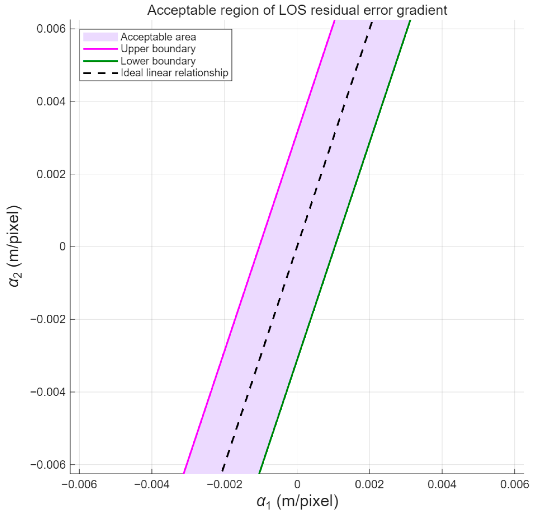
First, perpendicular baseline $B_{\perp 1}$ = 0.1 m, and $B_{\perp 2}$ = 0.3 m is assumed. Figure 2 shows the acceptable region using (15) and the varying LOS residual-error slopes (gradients) $a_1$ and $a_2$. The horizontal and vertical axes represent the LOS residual-error slopes along the azimuth direction for the short and long baselines, $a_1$ and $a_2$, respectively, with units of m/pixel. The black dashed line corresponds to the ideal case where the slopes of the two baselines fully satisfy the geometric proportion of $a_2={\displaystyle \frac{B_2}{B_1}}{a}_1$. The purple lines give the upper and lower boundaries in (15), and the light shaded area between the two lines is the acceptable region where the CRT phase-gradient estimation does not experience jumps in the modulus sense. Figure 2 indicates that when the wavelength is 0.0125 m and a1 is 0, the allowable width in the longitudinal direction is 0.0063 m. Exceeding this range means that the CRT will wrongly project the phase gradient to the adjacent modulus, thereby causing elevation estimation errors, and the resulting height error will be one or multiple times the ambiguity height. For example, under the K-band and long-baseline configuration in this paper, the ambiguity height calculated is 4.13 m. Figure 2 indicates that once the difference of the residual phase gradient violates the constraint of λ/4, even if only a single 2π phase wrap occurs in the adjacent pixels, causing the CRT to misjudge the ambiguity number by ±1, the error propagated to the elevation domain will be a height error of ±4.13 m. This is undoubtedly disastrous. This result quantitatively explains the high sensitivity of the CRT phase gradient to small residual motion errors in high-frequency unmanned aerial vehicle multi-baseline InSAR.

2.2. Low-Order Phase-Error Compensation Algorithm

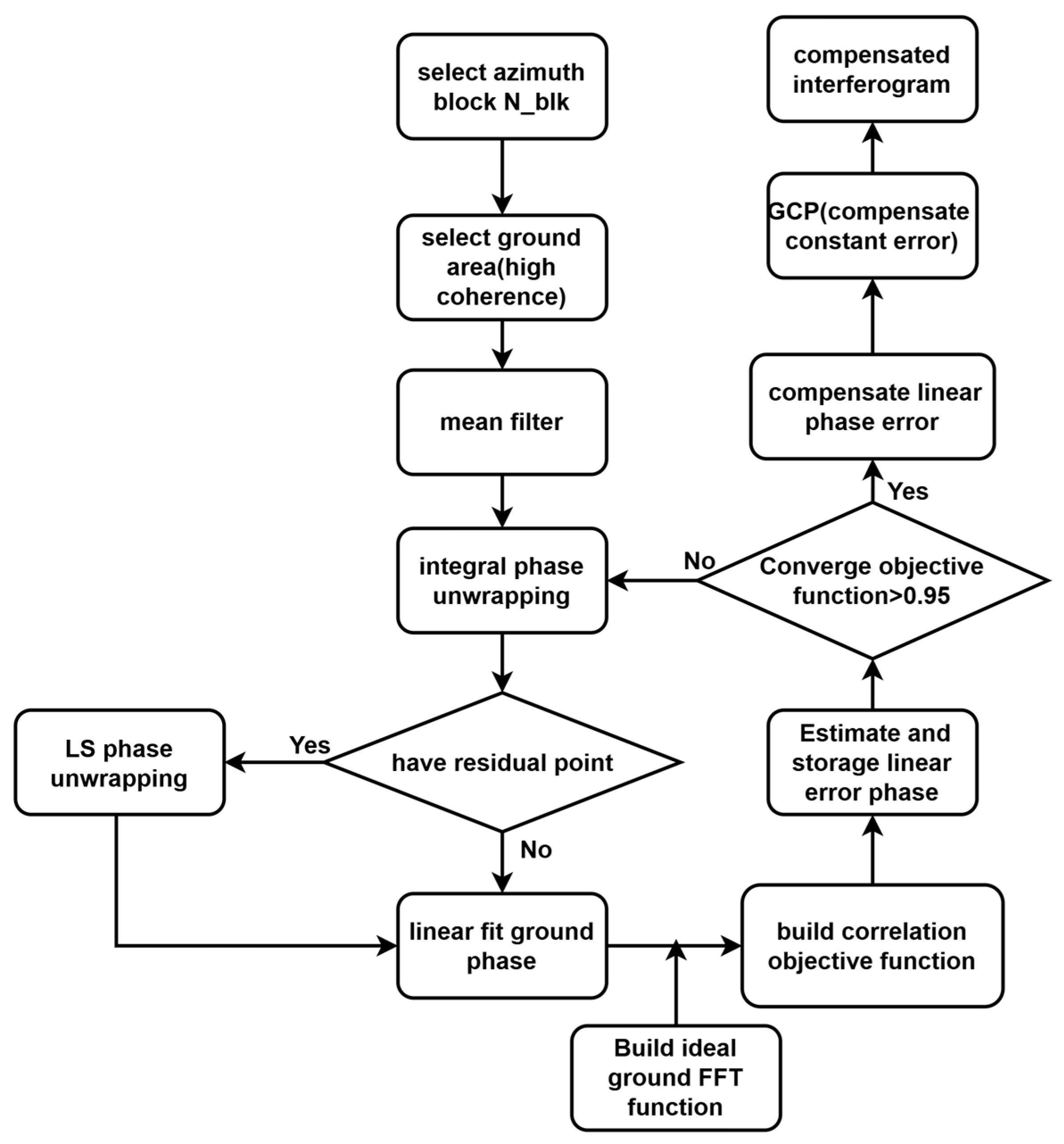
As described in Section 2.1, in complex terrains, the large variation in height phase leads to an amplified impact of residual errors after autofocus, thereby causing more misjudgments by the CRT and reducing the system’s performance. The proposed algorithm is applied after autofocus, using the image after autofocus and the resulting interferogram as input. Although the quality of autofocus will directly affect the residual phase structure model, some processing is used in our algorithm to enhance robustness. To address the influence of low-order motion errors on the interferometric phase, a parameterized linear-error phase estimation method is proposed. In the algorithm shown in Figure 3, the master and slave images after autofocus are first input. After co-registration of the images, an interferogram is obtained. Then, the interferogram is divided into multiple blocks in the azimuth direction, each with a pixel count of $N_{blk}$. In this paper, the interferogram is divided into 64 azimuth blocks, each with 4096 pixels. Next, a local coherence map is calculated for each block, and the ground area is selected by maximizing the average coherence within the ground mask. Based on experience, ground areas with an average coherence lower than 0.7 are skipped. Then, a 7 × 7 sliding window is used to perform mean filtering on the ground area to suppress speckle and high-order residual phase errors. Subsequently, one-dimensional integral phase unwrapping is performed along the azimuth direction. The phase continuity is detected by calculating the phase residuals, and for pixels with discontinuities, the unwrapped phase is estimated using least squares estimation. The ground phase after unwrapping is fitted with a linear model, and the spectral peak offset is estimated using the fast Fourier transform (FFT) to update the linear correction term. The correlation coefficient with the Fourier transform of the ideal ground phase is calculated using (19). If the correlation coefficient is less than 0.95, the one-dimensional integral phase unwrapping is iterated, and the estimated phase error of each iteration is stored. Otherwise, the process stops, and the block-level estimated value is stored. The maximum number of iterations is defined as 10. As a conservative criterion: values with a correlation coefficient lower than 0.95 are usually associated with high-order residual phase errors or unwrapping artifacts after autofocus, which can distort the sinc side lobes and potentially mislead the stop decision. After the iteration stops, the estimated and stored linear phase error is compensated into the interferogram after mean filtering. Then, GCP is used to estimate and compensate the constant phase error. Finally, the interferogram with low-order phase-error compensation is obtained.

For clarity, this paper provides Algorithm A1 in Appendix A to detail the implementation of each processing block shown in Figure 3.

This paper now describes the block-based phase-unwrapping step in Figure 3. The ground-area interferometric phase is first unwrapped by azimuthal integration so that residual post-autofocus errors do not introduce phase jumps that would bias the linear fit in (13). To enforce phase continuity when discontinuities are detected, a least squares (LS) refinement is then applied [30,31]:

$$\begin{array}{c}\min \hspace{1em}\hspace{1em}\hspace{1em}\sum {‖t(p,p-1)‖}_2\hspace{1em}\hspace{1em}\hspace{1em}\hspace{1em}\hspace{1em}\hspace{1em}\hfill \\ \hfill \phi \left(p\right)-\phi (p-1)-∆\phi (p,p-1)=t(p,p-1)\hfill \end{array}$$

(16)

Among them, $\phi \left(p\right)-\phi (p-1)$ is the continuous phase obtained by using the integral unwrapping under ideal conditions, and $∆\phi (p,p-1)$ is the phase jump caused by the residual phase error (the actual measured value). ${‖t(p,p-1)‖}_2$ represents the sum of the phase differences representing the positions of all residual points with a norm of 2 is ideally zero. Finally, let (16) converge to achieve the continuous phase in the ground area.

Under ideal conditions, the spectral shape of the ground reference phase is given (which can be regarded as an ideal sinc template or a center-aligned reference spectrum), providing a criterion for the residual linear phase error to be estimated:

$$F_i=FFT\left\{\mathit{exp}\left(jz\right)\right\}\hspace{1em}z\in [-\pi ,\pi ],$$

(17)

Here, the ground phase is modeled as a constant, which may take an arbitrary value and therefore contributes an unknown constant offset. At this stage, this paper focuses on compensating the linear term; the constant term is addressed later. By Fourier transform properties [31], the ideal ground spectrum should exhibit a standard sinc shape, and after normalization its peak (0 dB) is centered at 0 Hz.

A linear fit is performed on the estimated linear-error phase and the phase after autofocusing in (13), followed by a fast Fourier transform:

$$F_e\left(i\right)=FFT\{\mathrm{e}\mathrm{x}\mathrm{p}[j·fit({\displaystyle \frac{4\pi }{\lambda }}(∆R_0+r_n^{err}\left(i\right)+r_{res}(i)))]·\mathrm{e}\mathrm{x}\mathrm{p}(-j·{phase\mathrm{ }}_{est})\}$$

(18)

Among them, the first complex exponential on the right side of the equation is the actually measured interferometric phase. It includes the terrain interference range $∆R_0$, residual low-order phase error $r_n^{err}\left(i\right)$ (to be estimated), and residual high-order phase error $r_{res}\left(i\right)$. The second complex exponential denotes the unknown phase term targeted for estimation and compensation, which is a vector varying with the azimuth index $i$. Ideally, when the phases varying with the slow time in the two complex exponentials cancel each other out, there will only be a constant phase term in the complex exponential. According to the properties of the Fourier transform, if there is still residual linear error, it will cause the sinc function to shift on the frequency axis. The relevant objective function is given by:

$$C={\displaystyle \frac{\sum _{i=1}^m\left|F_e\left(i\right)\right|·\left|F_i\right|}{\sqrt{\sum _{i=1}^m{\left|F_e\left(i\right)\right|}^2\sum _{i=1}^k{\left|F_i\right|}^2}}}$$

(19)

where $m$ represents the number of sampling points on the azimuth of the ground region selected. $C$ denotes the correlation coefficient of the two sinc functions under the ideal ground condition and after linear-error compensation. In an ideal situation, Equation (19) converges to 1, indicating that the linear error has been compensated. In practice, it is difficult to converge to 1. Therefore, this paper designs to increase the number of sampling points in (17) and (18) as much as possible to enhance the accuracy of the compensation. To prevent a discontinuous phase from occurring during the least squares unwrapping process with a norm of 2, this paper sets up an iteration. The condition for judgment is that if the correlation coefficient is less than 0.95, the least squares unwrapping is performed again, as shown in Figure 3. Then, the stored phases are added to compensate the entire interferogram. From a physical perspective, Equation (17) indicates that the ideal value of the velocity error ${\displaystyle \frac{B_2}{B_1}}{a}_1-a_2$ under the different baselines in (15) is 0. Achieving maximum correlation in (19) implies that the difference in velocity errors of the two trajectories in $F_e\left(i\right)$ can be estimated through this.

After the linear-phase-error compensation is completed, in addition to the original constant error, due to the arbitrary setting of $z$ in (17), a constant error is added. Therefore, in the last step of Figure 3, this paper uses GCP to agree to compensate for all the constant errors.

The proposed procedure involves block-wise linear fitting, FFT-based peak-offset estimation, and a simple correlation stopping rule. These operations are computationally lightweight. Consequently, the method is compatible with near-real-time or onboard processing, provided that platform constraints on computing resources and data throughput are satisfied.

3. Simulation-Based Evaluation

This paper validates the proposed low-order phase-error estimation and compensation method after auto-focusing through the following approaches: (1) ideal multi-baseline simulation (the upper limit of the accuracy of the baseline digital elevation model); (2) injecting a known first-order (azimuth linear) residual term to exceed the λ/4 tolerance to trigger a CRT analog-to-digital error; (3) applying the proposed Motion compensation (MOCO) and GCP compensation to restore the correct ambiguity gradient and digital elevation model accuracy.

In this section’s simulation, this paper incorporates constant and linear phase errors using (12) and (13), and then applies Figure 3 from Section 2 and Algorithm A1 to compensate for the constant and linear phase errors in the interferogram.

A.

Ideal case multi-InSAR

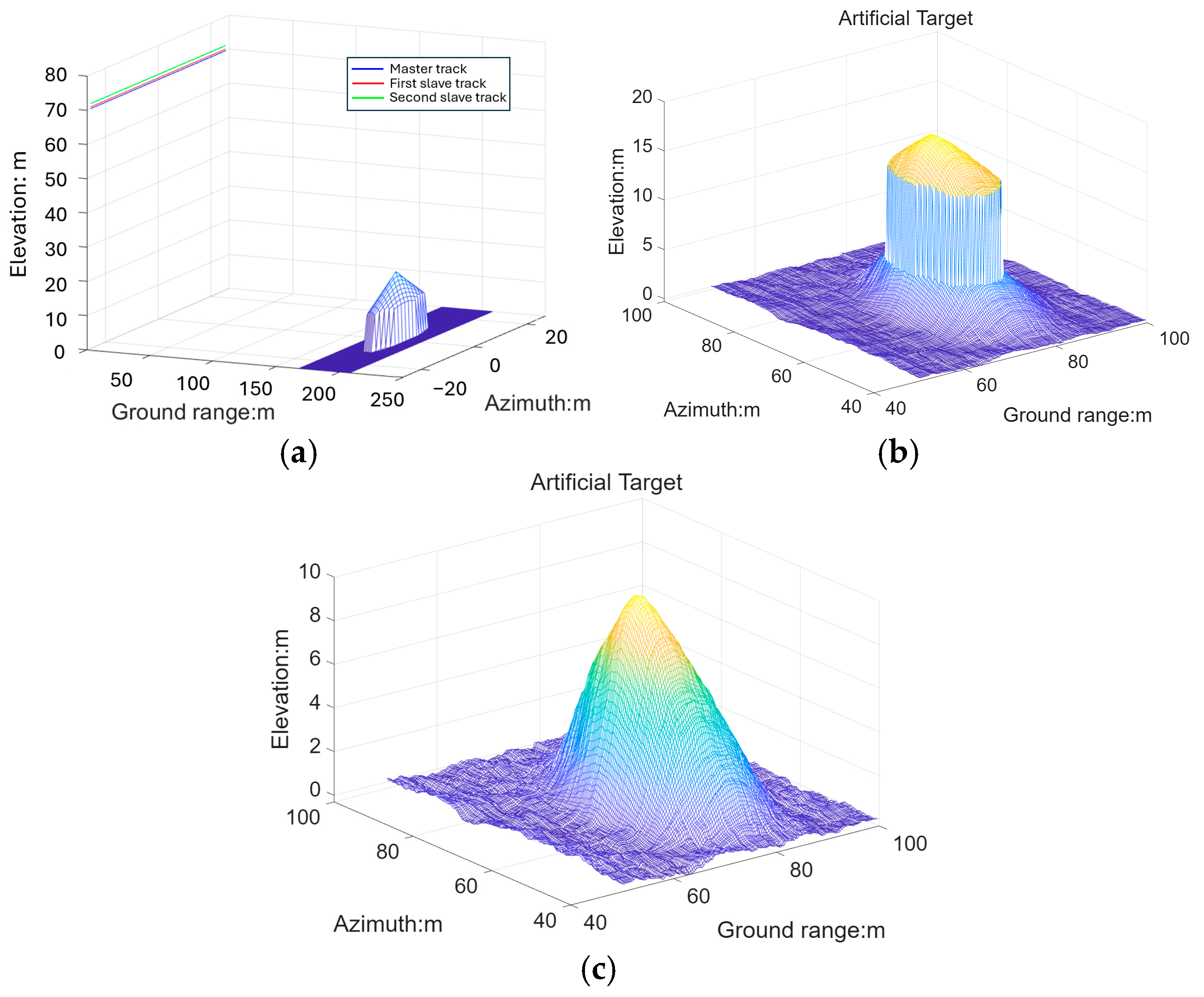
This paper first constructs a synthetic three-dimensional scene consisting of a cone on flat ground. To highlight differences between multi- and single-baseline processing, a 10 m height step is added to the cone, as shown in Figure 4a. The UAV performs three ideal straight-track flights (no injected errors), with the master track at 70 m altitude and two slave tracks at 70.1 m and 70.3 m. This configuration yields short and long perpendicular baselines of 0.1 m and 0.3 m, respectively. Simulation radar parameters are listed in

Table 3. Radar parameters.

Parameter	Value
Work Frequency	24 GHz
Bandwidth	1 GHZ
Azimuth Beamwidth	12.6°
Elevation Beamwidth	76.5°
Tx/Rx Antenna Gains	13.2 dBi
Transmit Power	8 dBm
Tx and Rx Channels	1-Tx, 1-Rx
Incidence Angle: $\theta$	70-degree
$\mathrm{Range} \mathrm{Resolution}: ∆R_g$	0.15 m
$\mathrm{Baseline} \mathrm{Angle}: \beta$	90°
$\mathrm{Wavelength}: \lambda$	0.0125 m
$\mathrm{Master} \mathrm{Trajectory} \mathrm{Range}: R_1$	211 m

. An ideal DEM is reconstructed using the multi-baseline processing chain in [31] and the multi-baseline phase-unwrapping method in [30], as shown in Figure 4b. For comparison, Figure 4c reports the DEM obtained using the single-baseline pipeline in [31]. The multi-baseline approach explicitly estimates ambiguity-number gradients between neighboring pixels, which is crucial around discontinuities such as the added step. In contrast, the single-baseline method assumes phase continuity across pixels [31], producing overly smooth height transitions. Quantitatively, the RMSE is 0.231 m for Figure 4b and 3.068 m for Figure 4c, demonstrating that the ideal multi-baseline setup can achieve decimeter-level DEM accuracy in the absence of motion errors.

Before addressing low-order residual phase terms, higher-order motion errors must be mitigated because they can defocus the SAR image [5]. Accordingly, this paper adopts the advanced autofocus method in [22] to compensate space-variant phase errors. After autofocus, this paper assumes that only a small high-order residual remains and that low-order (linear and constant) components dominate the residual phase error.

B.

Add Low-order residual phase error and apply Algorithm A1 compensation

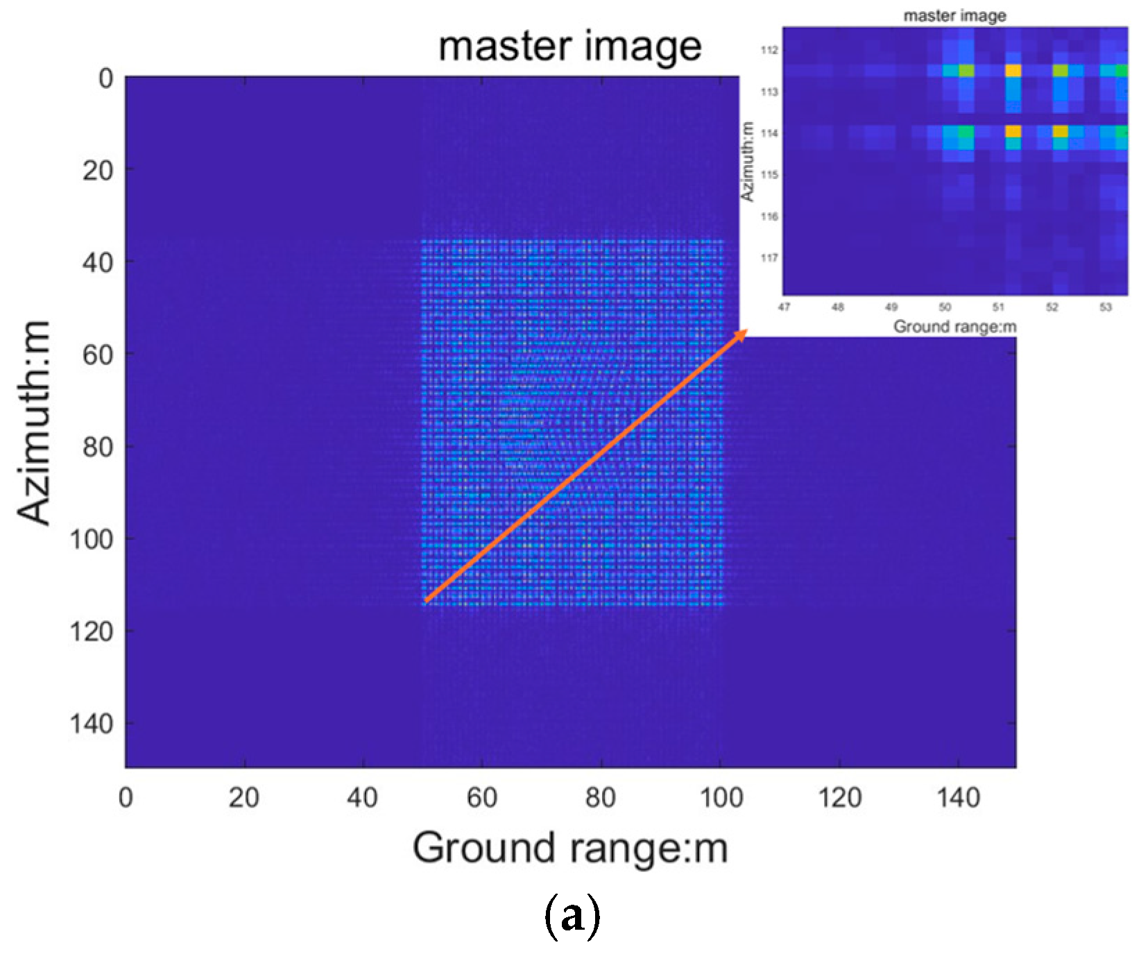
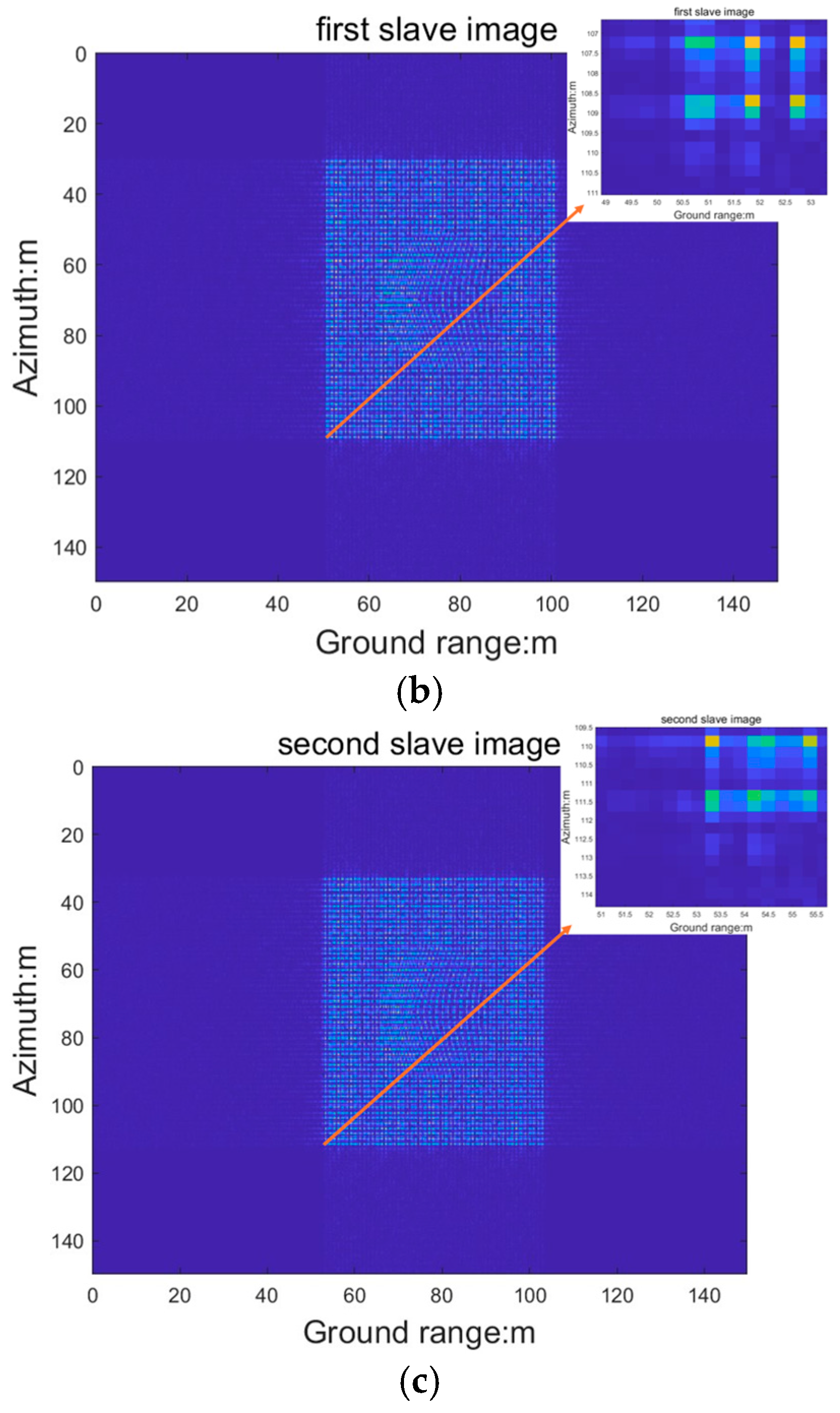
Next, this paper adds low-order motion errors to the LOS directions of the master and two slave trajectories, making the a1 of the interferograms of the small baseline and large baseline 0.06 m/pixel and 0.16 m/pixel, respectively. Through (15), the value of $\left|{\displaystyle \frac{B_2}{B_1}}{a}_1-a_2\right|$ is calculated to be 0.05 m, which is 16 times the quarter wavelength of this system. Permanent scatterers [32] will not be affected by spatial decorrelation and thus will not produce corresponding phase fluctuations. To highlight the impact of motion errors only, this paper uses a point target matrix as the permanent scatterer to perform two-dimensional restoration of the target in Figure 4a, as shown in Figure 5. Figure 5a, Figure 5b, and Figure 5c, respectively, display the master image and the two slave images. According to Table 3, the range resolution is 0.15 m, and the ground range resolution $∆x_h$ is calculated to be 0.33 m based on $∆x_h=∆R_g/sin\theta$. and incidence angles of 30°. Meanwhile, this paper sets the azimuth resolution to 0.33 m. The measurement ranges are: ground range (0 to 150 m), azimuth (0 to 150 m). To emphasize the target imaging part and reduce the computational load, this paper only adds point targets in the azimuth (38 m to 115 m) and ground range (50 m to 100 m) regions to describe the target area. Due to the baseline, the point target matrices in the master and two slave images in Figure 5 will have displacements in the range direction. As clearly stated in Figure 4a, the length and starting point of the synthetic aperture are the same, so the point target matrices should not have displacements in the azimuth direction. However, by comparing Figure 5a–c, it is found that the position of the point target in the lower left corner of the point target matrix in the azimuth direction is also different. This is because the velocity (linear) error in the LOS direction discussed in [5] will cause the image to have a displacement in the azimuth direction, which means that the three images in Figure 5 have different linear errors.

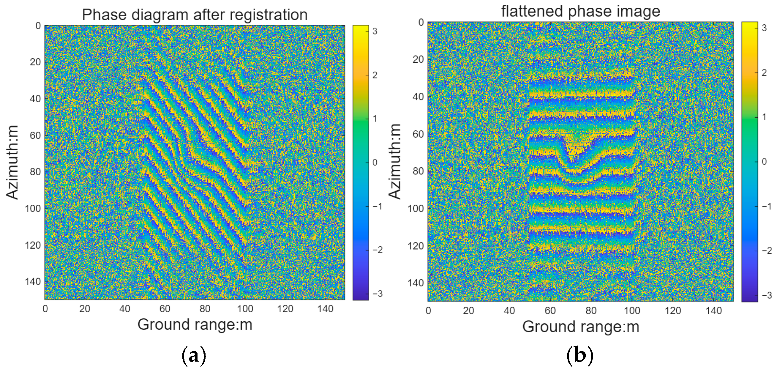
The two slave images are then co-registered to the master image using the time-domain correlation approach in [31]. The method searches over sub-pixel shifts within a predefined window (up/down/left/right), records the correlation for each shift, and selects the shift that maximizes correlation. For Figure 5a,b, the correlation improves from 0.235 to 0.98 after registration; for Figure 5a–c, it improves from 0.159 to 0.967. The registered slave image is then conjugate-multiplied with the master to form an interferogram. Because the long baseline provides higher height sensitivity in (2) [31], this paper shows only the long-baseline interferogram in Figure 6. In Figure 6a, the flat-ground region exhibits nearly uniform fringes, consistent with the weak spatial variability of low-order motion errors.

Over the conical target, fringes become denser due to the stronger topographic phase variation. Figure 6b shows the interferogram after flat-earth removal; at this point, the dominant remaining fringe pattern is driven by the residual linear error, which varies primarily along the azimuth over the ground region.

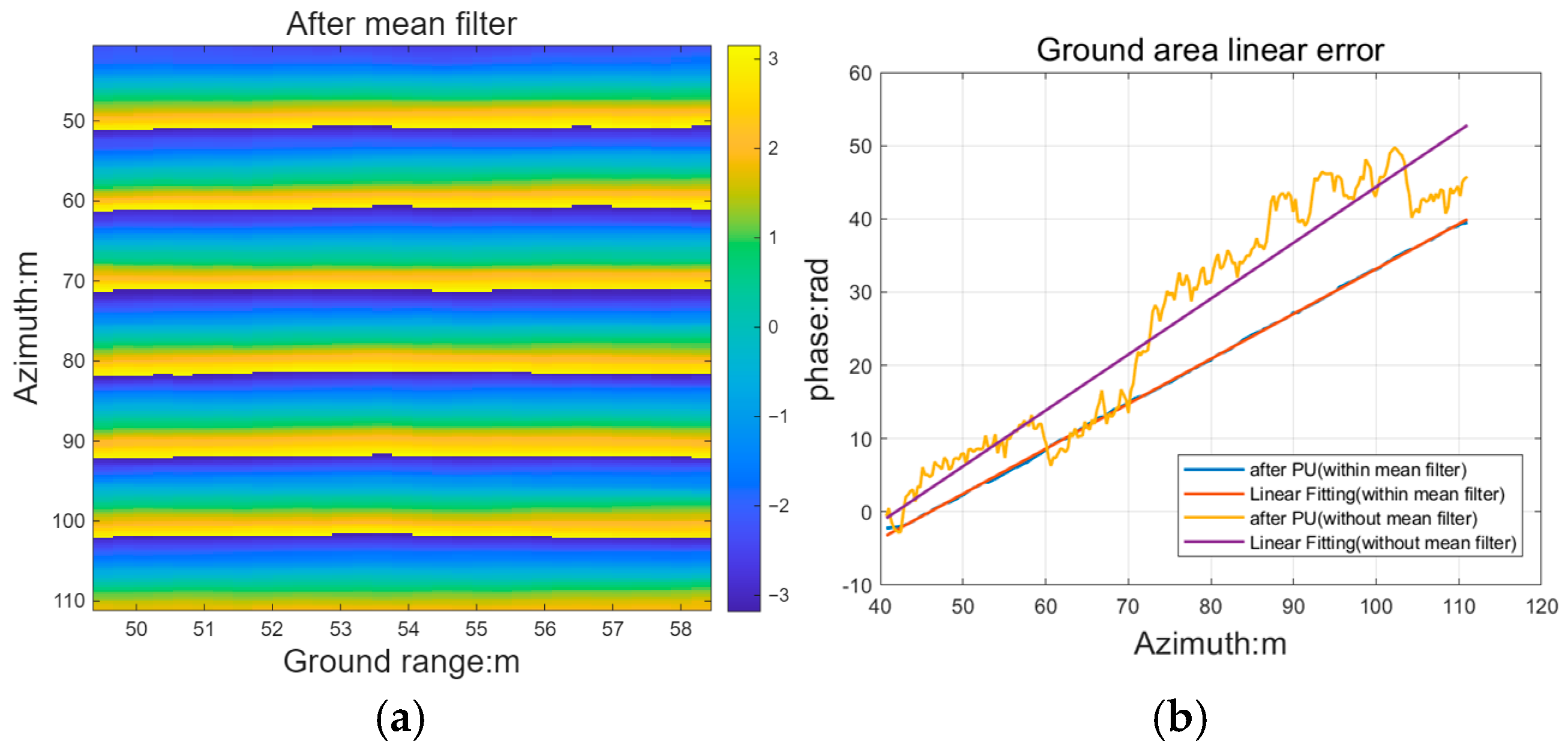
In coherent SAR imaging, echoes from many sub-resolution scatterers add with random phases, producing speckle. Together with post-autofocus residual phase errors, this leads to noticeable phase fluctuations in Figure 6. To make the ground region more suitable for low-order parameter estimation, this paper smooths the wrapped phase using a mean filter, which suppresses speckle and high-frequency residuals. A sliding-window implementation is used, and in this work, a 7 × 7 window is selected. The window-averaged phase is assigned to the center pixel as the window scans the image. The resulting mean-filtered ground-area interferogram is shown in Figure 7a.

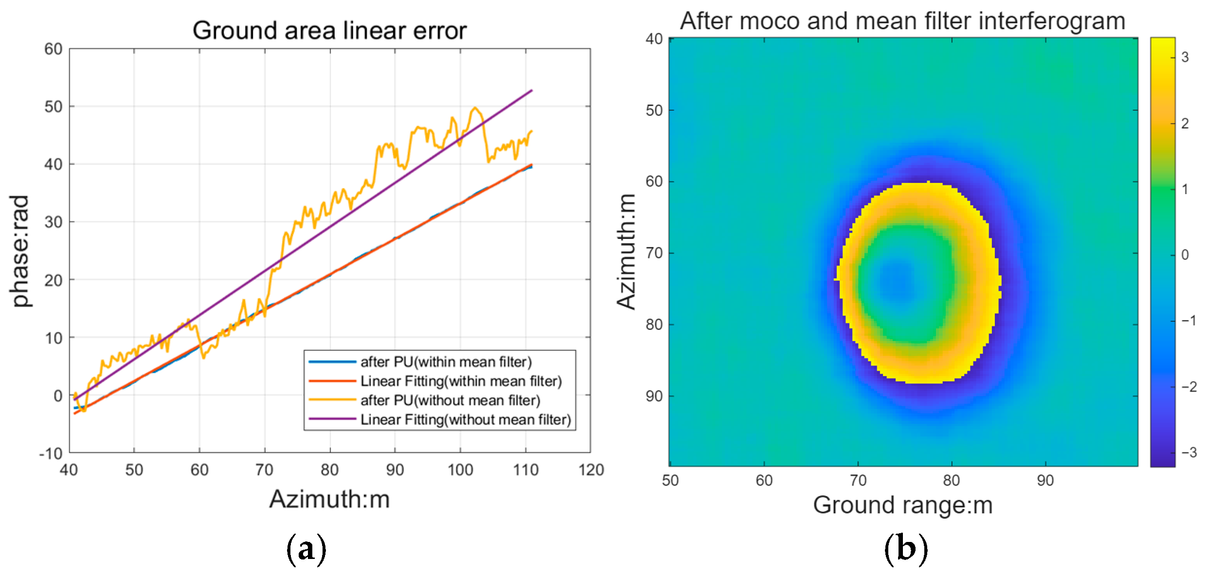
Comparing Figure 6 with Figure 7a highlights that mean filtering substantially attenuates speckle and irregular post-autofocus phase fluctuations, while preserving the overall wrapped-fringe trend. For unwrapping, this paper first detects phase residues [31], where each residue indicates a local ±2π inconsistency between neighboring samples. Azimuthal integration unwrapping is applied in residue-free regions, whereas LS estimation is used around residues to enforce phase continuity [31]. Figure 7b plots the unwrapped phase along one representative ground range bin: the yellow curve corresponds to no mean filtering, and the blue curve corresponds to the mean-filtered case. Although no explicit ±2π jumps are detected in the unfiltered (yellow) profile, speckle and residual errors introduce strong irregular fluctuations, which bias the subsequent linear fit. After mean filtering, the phase profile is much closer to a straight line, leading to a more reliable slope estimate (red line) than that obtained without filtering (purple line).

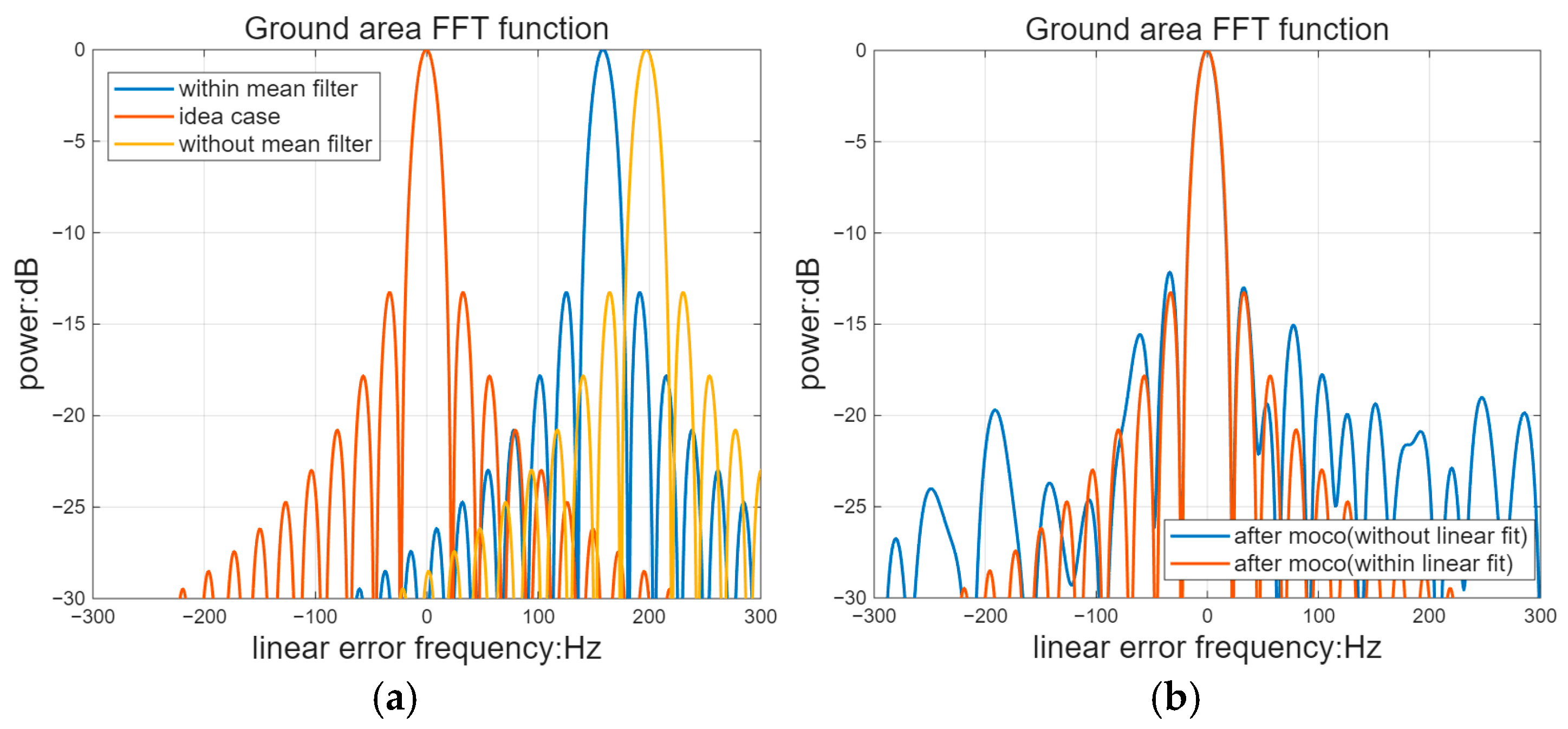
By setting $z$ to 0 in (17), this paper obtained the red standard sinc function in Figure 8 (with side lobes at −13 dB). Since the part within the complex exponential in (17) is constant, the linear-error frequency in Figure 8 is 0 Hz. To estimate the phase-error compensation, that is, the second part of (18), this paper only retained the second part of (18) and performed an FFT on it, for example, $FFT\left\{\exp \left(-j·{phase}_{est}\right)\right\}$. By substituting the purple data in Figure 7b into $FFT\left\{\exp \left(-j·{phase}_{est}\right)\right\}$, this paper calculated the yellow sinc function after linear fitting without mean filtering in Figure 8a. Meanwhile, by substituting the red data in Figure 7b into $FFT\left\{\exp \left(-j·{phase}_{est}\right)\right\}$, this paper calculated the blue sinc function after linear fitting with mean filtering in Figure 8a. Comparing the blue and yellow sinc functions in Figure 8a, it can be seen that the yellow data has a different linear frequency due to the absence of mean filtering, which makes it inaccurate. This paper substituted the ground area a range bin selected in Figure 6b into the first part of (18) and assumed that the first part of (18) did not use linear fitting. In Figure 8b, the blue data represents the FFT function of the ground area after motion compensation. In Figure 8b, the results of the ground area function with and without linear fitting processing are shown, both of which are calculated by (18). The curve without linear fitting also shows a linear trend, but due to speckle, it is not a straight line, as shown by the yellow curve in Figure 7b. At this time, the blue sinc function in Figure 8b is obtained by calculating (18). Figure 6b contains speckle and residual phase errors after autofocus. Since no linear fitting was used, it can be seen that the purple data is not a standard sinc function, and the random phase errors contained in it affect the power of the side lobes. This directly affects the judgment in Figure 3. For example, the linear-error frequencies of the purple data and the ideal red data in Figure 8 are both 0 Hz, but when they are substituted into (19), the correlation coefficient is 0.932, which is less than the 0.95 set in Section 2. This means that although the linear-error estimation is accurate at this time, the Figure 3 algorithm cannot determine the accuracy of the estimation due to the existence of random phase errors, leading to continuous iteration. Therefore, this paper substituted the linearly fitted ground area a range bin selected in Figure 6b into the first part of (18) for linear fitting. Then, this paper substituted the linear fitting data of the blue sinc function into the second part of (18) to calculate $F_e\left(i\right)$, as shown by the green sinc function in Figure 8. After calculation, the objective function (19) converges to 0.99. Since this paper used a mean filter to estimate the phase error and performed linear fitting on the data to be compensated, the algorithm effect shown in Figure 3 is significant, so no iteration was used.

Next, this paper extends the 1-D slope estimate (red curve in Figure 7b) into a 2-D phase-error map whose azimuth length matches Figure 7a and whose fringe spacing is consistent with Figure 6b, as illustrated in Figure 9a. This paper then extracts a window from Figure 6b with the same size as Figure 9a and applies complex-domain compensation by multiplying the corresponding complex exponentials. The compensated interferogram is shown in Figure 9b, where an elliptical phase pattern becomes visible and phase variation concentrates toward the ellipse center. Finally, this paper verifies whether this compensation level satisfies the CRT admissible region specified by (15).

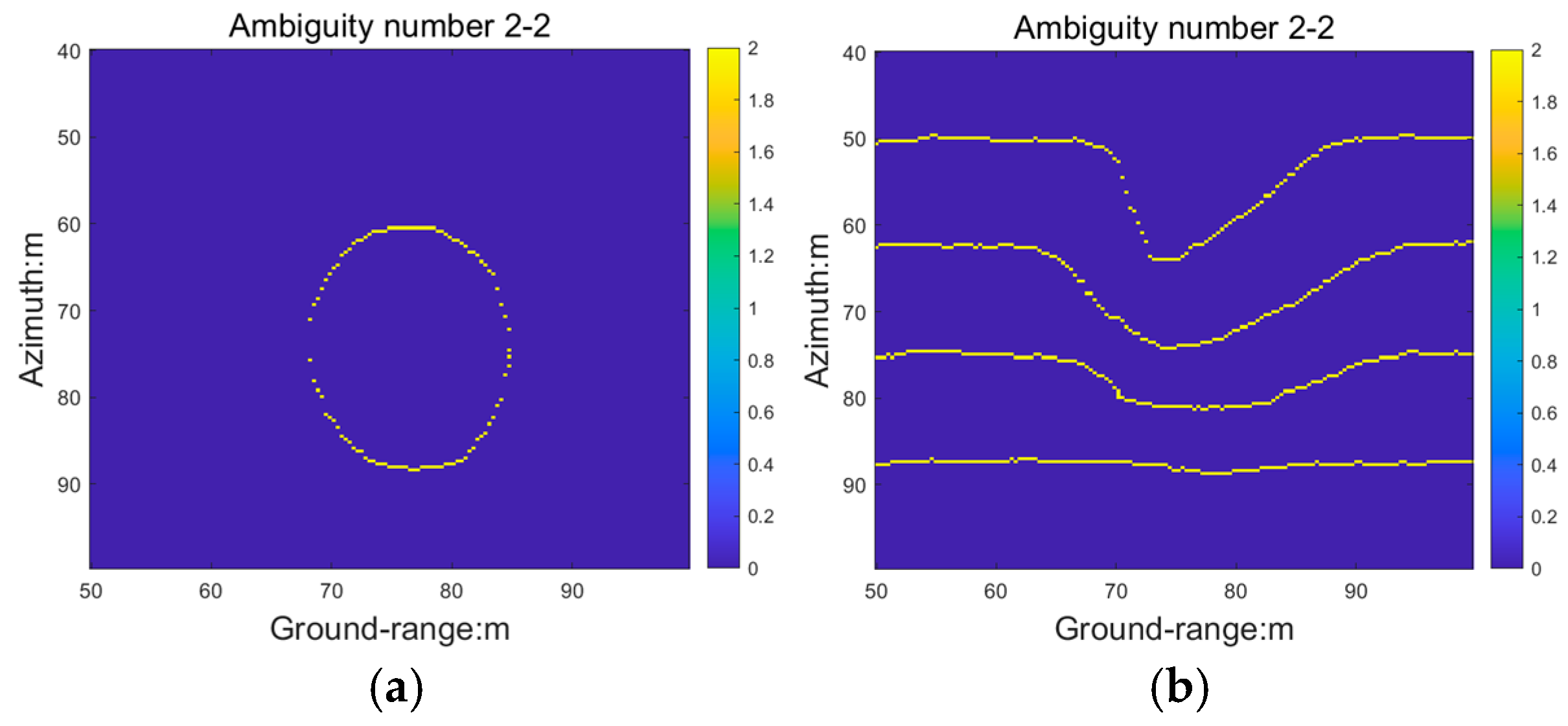
Applying TSPA to Figure 9b produces the ambiguity-number map in Figure 10a. The recovered ambiguity region forms a ring-shaped structure, consistent with the step-change footprint in Figure 4a. Using a 0.3 m perpendicular baseline, a 200 m ground range, and the parameters in Table 3, the ambiguity height is 4.13 m. The maximum ambiguity number can therefore be approximated as the maximum step height between adjacent pixels divided by the ambiguity height. With a 10 m step in Figure 4a, the expected maximum ambiguity number is 2, matching Figure 10a. Figure 10b shows the ambiguity numbers estimated without low-order compensation. The CRT clearly misclassifies ambiguity bands, consistent with the distorted fringe structure observed in Figure 6b.

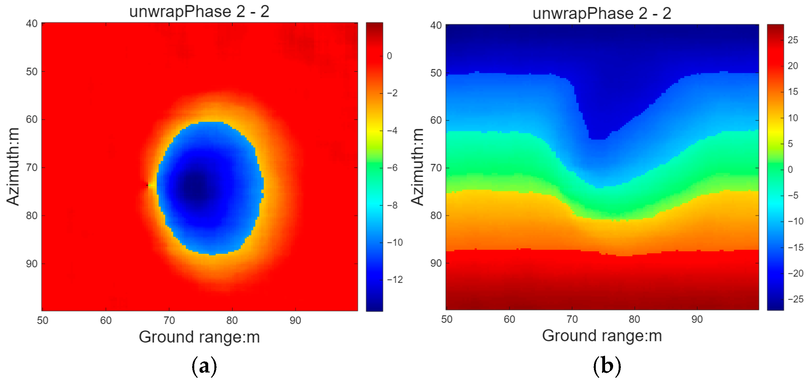
After obtaining the ambiguity numbers in Figure 10a, TSPA completes phase unwrapping using the minimum-cost flow algorithm [30], yielding Figure 11a. In Figure 11a, the ground region is near 1 rad, while the target step spans approximately 1 rad down to about −12 rad. Dividing the step-phase difference by 2π gives two full 2π cycles with a remainder of 0.433 rad, indicating an ambiguity number of 2—consistent with the ambiguity-height calculation and the ambiguity-number map. Without low-order compensation, Figure 11b shows an almost purely linear phase ramp. Because the CRT wrongly assigns ambiguity number 2 across multiple fringe boundaries (four such curves in Figure 10b), the unwrapped phase range becomes roughly 50.2 rad, as seen in Figure 11b.

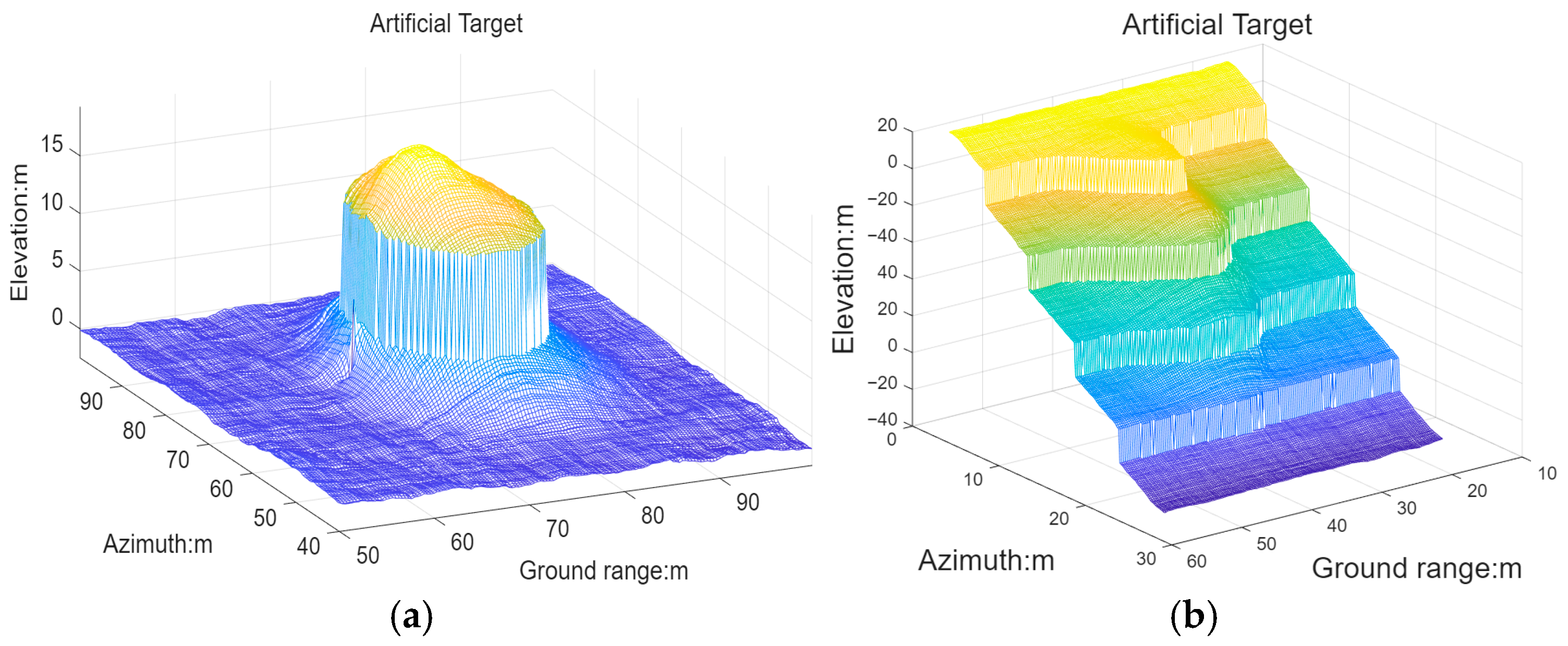
Substituting the unwrapped phases in Figure 11 into (2) produces the DEMs in Figure 12. Figure 12a,b correspond to results with and without the compensation algorithm of Figure 3, respectively. This paper computes the height RMSE by comparing each reconstructed DEM to the ground-truth DEM in Figure 4a. With compensation, the RMSE is 0.23 m, whereas without compensation, it increases dramatically to 42.3 m.

These simulations reproduce the primary failure mechanism observed in practice: once the λ/4 tolerance is violated, CRT-based ambiguity-gradient estimation can jump to an adjacent modulus, leading to large elevation errors. Real measurements further contain non-ideal coherence variations, for example, outliers due to shadowing and rapid terrain changes, which make residuals less regular. The proposed design—block processing, high-coherence profile selection, and an iterative correlation-based objective—aims to maintain robustness under such non-ideal conditions.

C.

Exploring the influence of system boundaries and autofocus compensation

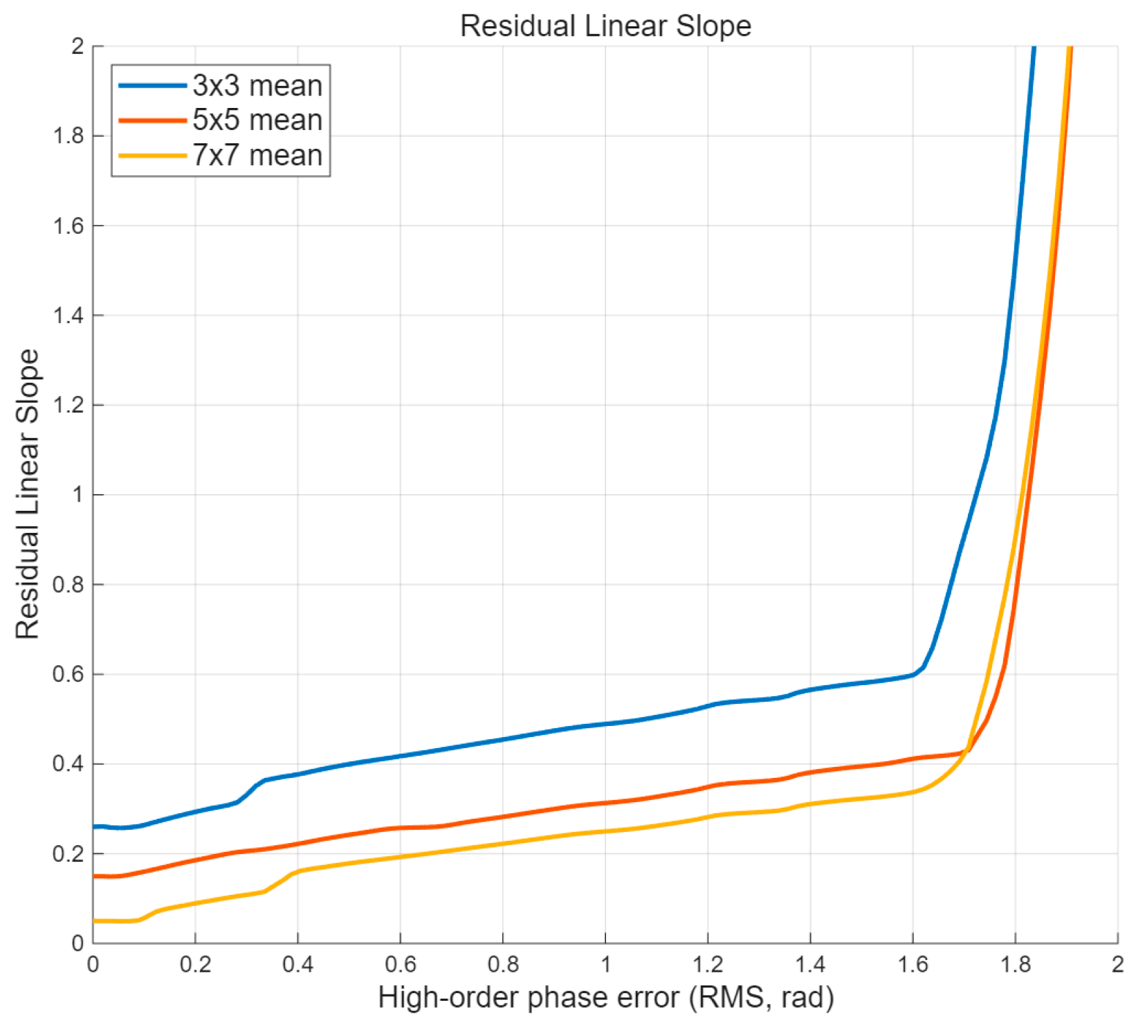
To explore the performance boundary of this algorithm and the impact of image quality after autofocus compensation on this algorithm, before applying the algorithm in Figure 3, high-order phase errors are added to the interferogram calculated in (18) to simulate the change in image processing quality caused by autofocusing. First, this paper presents a parameter that can quantify the performance of the algorithm in Figure 3. The performance parameter is given by:

$${RLS}_{RMS}=\sqrt{{\displaystyle \frac{1}{N_i}}{\sum }_i{(k\left(i\right)-G_{ture})}^2}$$

(20)

where ${RS}_{RMSE}$ represents the standard deviation of the residual slope. i is the range bin, $k\left(i\right)$ is the residual linear slope of the ground area fitted for each range bin, and $G_{ture}$ is the actual slope value of the ground area. Continuously increasing the higher-order phase error and using Figure 3, followed by 30 Monte Carlo simulations, we obtain Figure 13. The x-axis of Figure 13 is the standard deviation of the added higher-order phase error, and the y-axis is the residual linear slope of the ground area after the compensation of Figure 3, under different sizes of mean filter sliding windows. The ${RS}_{RMSE}$ remains unchanged at first and then shows an exponential growth at different standard deviations of higher-order phase errors. From this, the threshold of the performance of the Figure 3 algorithm under different sliding windows can be obtained. For example, under a 3 × 3 sliding window, the system performance drops significantly and is even completely destroyed when the standard deviation of the higher-order phase error is 2.1 rad. And due to the different suppression effects of different-sized windows on high-frequency phase errors, the inflection points and starting points of each curve are different. For instance, when the system threshold under a 7 × 7 window is 2.2 rad, and when no additional higher-order phase error is added, as the window size increases, the speckle can be better suppressed, resulting in more accurate linear fitting results. Thus, the ${RS}_{RMSE}$ is approximately 0.06 under a 7 × 7 window.

To explore whether the mean filter would distort the phase of low-frequency and slowly varying terrain, this paper established the following phase model:

$${\phi }_n^G={\phi }_n^{err}+{\phi }_n^{LF}+{\phi }_n^{noise}$$

(21)

${\phi }_n^G$ provides the winding phase on the ground area. ${\phi }_n^{err}$ is the phase of displacement and velocity error, ${\phi }_n^{LF}$ is the terrain phase of low-frequency variation, and ${\phi }_n^{noise}$ is the higher-order residual phase error mentioned above. The form of the phase in ${\phi }_n^{LF}$ is a sine function, and thus the variation of ${\phi }_n^{LF}$ is determined by the amplitude A and wavelength L of the sine function.

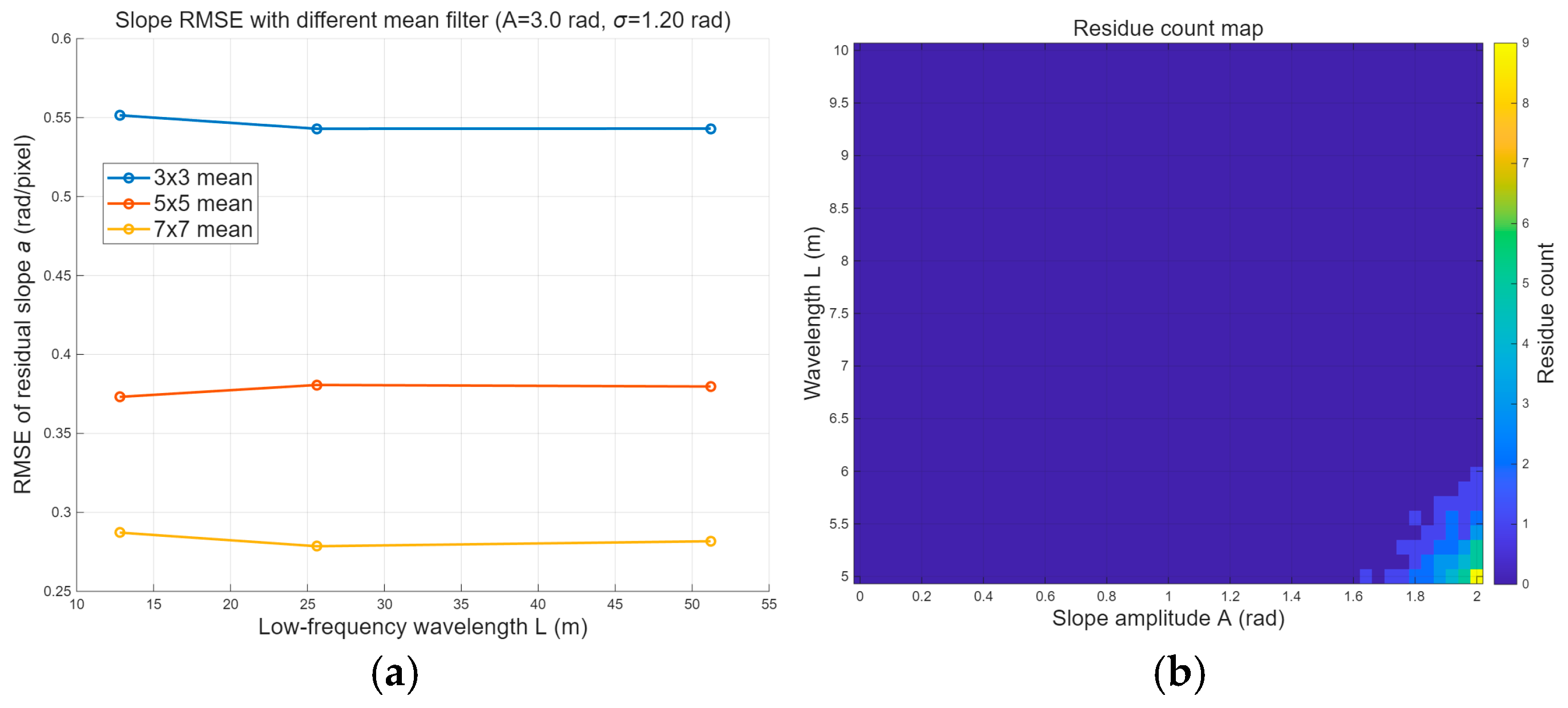
Substitute A as 3 rad, the standard deviation of the high-order residual phase error as 1.2 rad, and the wavelength varying from 10 m to 50 m into (21), and then substitute the model in (21) into the slope value of the interferogram of the ground area obtained after iteration in Figure 3. Finally, calculate $G_{ture}$ based on the above parameters and substitute it into (19) to calculate the ${RS}_{RMSE}$ at this time, as shown in Figure 14. The horizontal axis of Figure 14a is the wavelength of the varying sine function, and the larger it is, the slower the terrain changes. The vertical axis represents the standard deviation of the residual slope. Figure 14a indicates that when the wavelength of the sinusoidal terrain phase increases, it does not affect ${RS}_{RMSE}$. By comparing Figure 13 and Figure 14a, it can be known that the low-frequency varying terrain phase is not dissolved and distorted by the mean filter. For example, in Figure 13, when the standard deviation of the high-order residual phase error is 1.2 rad, the ${RS}_{RMSE}$ of 3 × 3, 5 × 5, and 7 × 7 are 0.57 rad, 0.38 rad, and 0.27 rad, respectively, which are approximately equal to the ${RS}_{RMSE}$ of the three different window filters in Figure 14a. This means that most of the ${RS}_{RMSE}$ is caused by the high-order residual phase error.

This paper also examines whether the LS unwrapping step in Figure 3 could incorrectly treat slowly varying terrain phase as a discontinuity and thereby introduce extra errors. In Figure 3, LS unwrapping is triggered only when phase residues are present; if no residues exist (i.e., the interferogram phase is continuous), LS is not applied. Accordingly, this paper counts residues while fixing the high-order residual-error standard deviation to 1.2 rad and sweeping the sine-terrain wavelength L and amplitude A, as shown in Figure 14b. Most parameter combinations yield near-zero residue counts, implying continuous phase and no additional LS-induced error. As A increases and L decreases, residue counts rise (up to 9), and because LS fitting cannot perfectly match the ideal phase, additional unwrapping error may be introduced in this regime.

This section conducts the argumentation through a coherent chain of simulation verification: Firstly, a multi-baseline system is established under ideal error-free conditions to obtain the DEM. Then, low-order residual errors are injected into the interferogram to reproduce the error phenomenon and explain the convergence and iteration mechanism of the correlation coefficient objective function. Subsequently, the recovery effect of the DEM is evaluated using quantitative indicators. Finally, the intensity of high-order residual errors is further scanned to analyze the robustness boundary of the algorithm. The results show that low-order residual errors can cause modulus jumps in the CRT phase gradient, leading to a significant collapse in DEM accuracy. However, the method proposed in this paper estimates errors based on the FFT spectral peak offset, completes stable iterations by combining convergence criteria, and suppresses errors through linear term compensation (MOCO) and constant term correction (GCP), enabling the multi-baseline DEM to significantly restore accuracy within a certain autofocus quality range. Meanwhile, this section provides the robustness relationship between the mean filtering window size and the intensity of high-order residual errors, providing a basis for parameter selection and application scope.

4. Conclusions

This work investigates repeat-pass K-band UAV multi-baseline InSAR and systematically analyzes the low-order (linear and constant) residual motion-error phase that may remain after autofocus. Our analysis shows that the admissible line-of-sight (LOS) motion-error tolerance for reliable CRT phase-gradient estimation is on the order of one quarter wavelength. To mitigate violations of this tolerance, this paper proposes the low-order compensation procedure summarized in Figure 3 and detailed in Algorithm A1. The method estimates the residual linear term through block-wise linear fitting and FFT spectral peak-offset analysis, and uses a correlation objective (threshold 0.95) as a practical convergence criterion; a GCP-based step then removes the remaining constant phase bias. In simulation, different residual errors on the slave trajectories cause CRT failure and a dramatic increase in DEM error. After applying the proposed compensation, the objective converges to approximately 0.984 (close to 1) and DEM accuracy is restored, with RMSE approaching that of the error-free reference case. These results demonstrate that the proposed post-autofocus correction can recover large-scale mapping scenes to decimeter-level DEM accuracy under high-frequency UAV conditions.

For practical deployment, inertial measurement unit/global navigation satellite system (IMU/GNSS) observations can provide informative motion priors, easing the autofocus burden and stabilizing phase-error estimation [33]. The proposed method can then act as a data-driven post-correction stage to refine remaining low-order terms. In addition, learning-based strategies—such as Kalman filtering with IMU priors or recurrent models for phase denoising—may further improve robustness under low SNR and complex dynamics [33].

This paper also plans to develop a more explicit physics-based parametric model and solve it using regularized least squares or state-space estimation. These physical relationships can be introduced as constraints or penalty terms in a physics-informed neural network (PINN), enabling hybrid physics–data estimation under more challenging noise and motion conditions.

Finally, in cooperative or swarm UAV operations, multi-platform observations can provide additional baselines and redundancy. Cross-platform consistency constraints may further suppress low-order residuals. In this context, the proposed post-autofocus low-order compensation can be integrated as a modular block within a cooperative processing pipeline alongside synchronization, co-registration, and joint multi-baseline unwrapping.

References

1. Rosen, P.A.; Hensley, S.; Joughin, I.R.; Li, F.K.; Madsen, S.N.; Rodriguez, E.; Goldstein, R.M. Synthetic aperture radar interferometry. Proc. IEEE 2000, 88, 333–382. [Google Scholar] [CrossRef]
2. Bamler, R.; Hartl, P. Synthetic aperture radar interferometry. Inverse Probl. 1998, 14, R1. [Google Scholar] [CrossRef]
3. Moreira, A.; Prats-Iraola, P.; Younis, M.; Krieger, G.; Hajnsek, I.; Papathanassiou, K.P. A tutorial on synthetic aperture radar. IEEE Geosci. Remote Sens. Mag. 2013, 1, 6–43. [Google Scholar] [CrossRef]
4. Cumming, I.G.; Wong, F.H. Digital Processing of Synthetic Aperture Radar Data; Artech House: Norwood, MA, USA, 2005. [Google Scholar]
5. Carrara, W.G.; Goodman, R.S.; Majewski, R.M. Spotlight Synthetic Aperture Radar: Signal Processing Algorithms; Artech House: Boston, MA, USA; London, UK, 1995. [Google Scholar]
6. Hanssen, R.F. Radar Interferometry: Data Interpretation and Error Analysis; Kluwer Academic Publishers: Dordrecht, The Netherlands, 2001. [Google Scholar]
7. Yu, H.; Li, Z.; Bao, Z. A cluster-analysis-based efficient multibaseline phase-unwrapping algorithm. IEEE Trans. Geosci. Remote Sens. 2011, 49, 478–487. [Google Scholar] [CrossRef]
8. Liu, H.; Xing, M.; Bao, Z. A cluster-analysis-based noise-robust phase-unwrapping algorithm for multibaseline interferograms. IEEE Trans. Geosci. Remote Sens. 2015, 53, 494–504. [Google Scholar]
9. Berardino, P.; Fornaro, G.; Lanari, R.; Sansosti, E. A new algorithm for surface deformation monitoring based on small baseline differential SAR interferograms. IEEE Trans. Geosci. Remote Sens. 2002, 40, 2375–2383. [Google Scholar] [CrossRef]
10. Yuan, Z.; Deng, Y.; Li, F.; Wang, R.; Liu, G.; Han, X. Multichannel InSAR DEM Reconstruction Through Improved Closed-Form Robust Chinese Remainder Theorem. IEEE Geosci. Remote Sens. Lett. 2013, 10, 1314–1318. [Google Scholar] [CrossRef]
11. Ullmann, I.; Bonfert, C.; Grathwohl, A.; Lahmeri, M.A.; Mustieles-Pérez, V.; Kanz, J.; Sterk, E.; Bormuth, F.; Ghasemi, R.; Fenske, P.; et al. Towards Detecting Climate Change Effects with UAV-Borne Imaging Radars. IEEE J. Microw. 2024, 4, 881–893. [Google Scholar] [CrossRef]
12. López, Y.Á.; García-Fernández, M.; Álvarez-Narciandi, G.; Andrés, F.L.-H. Unmanned aerial vehicle-based ground-penetrating radar systems: A review. IEEE Geosci. Remote Sens. Mag. 2022, 10, 66–86. [Google Scholar] [CrossRef]
13. Ding, M.-L.; Ding, C.-B.; Tang, L.; Wang, X.-M.; Qu, J.-M.; Wu, R. A W-Band 3-D Integrated Mini-SAR System with High Imaging Resolution on UAV Platform. IEEE Access 2020, 8, 113601–113609. [Google Scholar] [CrossRef]
14. Schreiber, E.; Heinzel, A.; Peichl, M.; Engel, M.; Wiesbeck, W. Advanced buried object detection by multichannel, UAV/drone carried synthetic aperture radar. In Proceedings of the 2019 13th European Conference on Antennas and Propagation (EuCAP 2019), Krakow, Poland, 31 March–5 April 2019; pp. 1–5. [Google Scholar]
15. Grathwohl, A.; Arendt, B.; Grebner, T.; Waldschmidt, C. Detection of Objects Below Uneven Surfaces with a UAV-Based GPSAR. IEEE Trans. Geosci. Remote Sens. 2023, 61, 5207913. [Google Scholar] [CrossRef]
16. Jean-Francois, N.; Nicolas, C.; Jérôme, H. SAR Imaging Challenges on UAV Trajectory Restitution Study Case with SAR-Light Prototype at X-Band. In Proceedings of the 2022 IEEE International Symposium on Inertial Sensors and Systems (INERTIAL), Avignon, France, 8–11 May 2022; pp. 1–3. [Google Scholar] [CrossRef]
17. Yan, J.; Guo, J.; Lu, Q.; Wang, K.; Liu, X. X-band mini SAR radar on eight-rotor mini-UAV. In Proceedings of the 2016 IEEE International Geoscience and Remote Sensing Symposium (IGARSS), Beijing, China, 10–15 July 2016; pp. 6702–6705. [Google Scholar] [CrossRef]
18. Mustieles-Pérez, V.; Kim, S.; Bonfert, C.; Krieger, G.; Villano, M. Towards UAV-Based Ultra-Wideband Multi-Baseline SAR Interferometry. In Proceedings of the 20th European Radar Conference (EuRAD 2023), Berlin, Germany, 20–22 September 2023; pp. 233–236. [Google Scholar] [CrossRef]
19. Dong, Y.; Jiang, H.; Zhang, L.; Liao, M. An Efficient Maximum Likelihood Estimation Approach of Multi-Baseline SAR Interferometry for Refined Topographic Mapping in Mountainous Areas. Remote Sens. 2018, 10, 454. [Google Scholar] [CrossRef]
20. Yu, H.; Xing, M.; Yuan, Z. Baseline Design for Multibaseline InSAR System: A Review. IEEE J. Miniat. Air Space Syst. 2021, 2, 17–24. [Google Scholar] [CrossRef]
21. Yu, H.; Lee, H.; Cao, N.; Lan, Y. Optimal baseline design for multi-baseline InSAR phase unwrapping. IEEE Trans. Geosci. Remote Sens. 2019, 57, 5738–5750. [Google Scholar] [CrossRef]
22. Bekar, A.; Antoniou, M.; Baker, C.J. Low-cost, high-resolution, drone-borne SAR imaging. IEEE Trans. Geosci. Remote Sens. 2022, 60, 5208811. [Google Scholar] [CrossRef]
23. Bekar, A.; Bekar, M.; Baker, C.J.; Antoniou, M. Coherent Change Detection for High-Resolution Drone-Borne SAR at 24 GHz. IEEE J. Sel. Top. Appl. Earth Obs. Remote Sens. 2024, 17, 84–94. [Google Scholar] [CrossRef]
24. Bekar, A.; Antoniou, M.; Baker, C.J. High-resolution drone-borne SAR using off-the-shelf high-frequency radars. In Proceedings of the 2021 IEEE Radar Conference (RadarConf21), Atlanta, GA, USA, 7–14 May 2021; pp. 1–6. [Google Scholar]
25. Bekar, A.; Antoniou, M.; Baker, C.J. Change Detection for High-Resolution Drone-Borne SAR at High Frequencies—First Results. In Proceedings of the 2023 IEEE Radar Conference (RadarConf23), San Antonio, TX, USA, 1–5 May 2023; pp. 1–5. [Google Scholar] [CrossRef]
26. Chuang, H.-Y.; Kiang, J.-F. An On-Site InSAR Terrain Imaging Method with Unmanned Aerial Vehicles. Sensors 2024, 24, 2287. [Google Scholar] [CrossRef]
27. Frey, O.; Werner, C.L. UAV-borne Repeat-pass SAR Interferometry and SAR Tomography with a Compact L-band SAR System. In Proceedings of the 13th European Conference on Synthetic Aperture Radar (EUSAR 2021), Online, 29–31 April 2021; pp. 181–184. [Google Scholar]
28. Ruiz-Carregal, G.; Cuenca, M.L.; Yam, L.; Masalias, G.; Makhoul, E.; Iglesias, R.; Heredia, A.; González, Á.; Centolanza, G.; Gili-Zaragoza, A.; et al. Ku-Band SAR-Drone System and Methodology for Repeat-Pass Interferometry. Remote Sens. 2024, 16, 4069. [Google Scholar] [CrossRef]
29. Yuan, Z.; Lu, Z.; Chen, L.; Xing, X. A Closed-Form Robust Cluster-Analysis-Based Multibaseline InSAR Phase Unwrapping and Filtering Algorithm with Optimal Baseline Combination Analysis. IEEE Trans. Geosci. Remote Sens. 2020, 58, 4251–4262. [Google Scholar] [CrossRef]
30. Yu, H.; Lan, Y. Robust Two-Dimensional Phase Unwrapping for Multibaseline SAR Interferograms: A Two-Stage Programming Approach. IEEE Trans. Geosci. Remote Sens. 2016, 54, 5217–5225. [Google Scholar] [CrossRef]
31. ESA. InSAR Principles: Guidelines for SAR Interferometry Processing and Interpretation; ESA Publications: Noordwijk, The Netherlands, 2007. [Google Scholar]
32. Alessandro, F.; Prati, C.; Rocca, F. Permanent scatterers in SAR interferometry. IEEE Trans. Geosci. Remote Sens. 2002, 39, 8–20. [Google Scholar]
33. Liu, B.; Liu, P.; Wang, Y.; Li, Z.; Lv, H.; Lu, W.; Olofsson, T.; Rabczuk, T. Explainable machine learning for multiscale thermal conductivity modeling in polymer nanocomposites with uncertainty quantification. Compos. Struct. 2025, 370, 119292. [Google Scholar] [CrossRef]
Figure 1. Multi-baseline geometry.
Mathematics 14 00772 g001
Figure 2. Acceptable region of LOS residual-error gradient.
Mathematics 14 00772 g002
Figure 3. Low-order phase-error estimation and compensation algorithm.
Mathematics 14 00772 g003
Figure 4. (a) Geometry model. (b) Ideal multi-baseline simulation result. (c) Ideal single-baseline simulation result.
Mathematics 14 00772 g004
Figure 5. (a) Master image. (b) First slave image. (c) Second slave image.
Mathematics 14 00772 g005aMathematics 14 00772 g005b
Figure 6. (a) After registration interferogram. (b) Flattened interferogram.
Mathematics 14 00772 g006
Figure 7. (a) Ground area after mean filter. (b) A ground range bin ground area.
Mathematics 14 00772 g007
Figure 8. Ground area FFT function: (a) ideal and have low-order phase error; (b) after phase compensation.
Mathematics 14 00772 g008
Figure 9. (a) Estimate linear phase error. (b) After moco interferogram.
Mathematics 14 00772 g009
Figure 10. (a) After moco long-baseline estimate ambiguity number. (b) Without moco long-baseline estimate ambiguity number.
Mathematics 14 00772 g010
Figure 11. (a) After moco long-baseline unwrapped phase. (b) Without moco long-baseline estimate ambiguity unwrapped phase.
Mathematics 14 00772 g011
Figure 12. (a) After moco long-baseline DEM. (b) Without moco long-baseline estimate DEM.
Mathematics 14 00772 g012
Figure 13. Boundary of compensation algorithm.
Mathematics 14 00772 g013
Figure 14. (a) Root mean square error of slope under different mean filters. (b) Residual count plot.
Mathematics 14 00772 g014