A Conceptual Model for Growth by Capital–Education Investments

Abstract

In a first approximation, economic growth depends on capital investments and on investments in education and innovation. The macro-economic model introduced here will specifiy aggregate output as determined by aggregate supply of capital and education investment. We will consider the effectiveness of education including its quality for the growth of the National Product. It is surprising that small changes in the quality of education have a considerable long-term impact on economic growth. Secondly, we consider the positive and negative influences of chaotic fluctuations of capital investments caused by hype cycles or erratic policies. Finally, we introduce a continuous control by consumption on education investments. In this three-dimensional macro-economic model, a tipping point exists where an increase in consumption affecting the amount of education and innovation leads to a decline in economic growth.

1. Introduction

Large parts of economic research are focused on the micro-management of the economy. This paper ignores such aspects to consider the long-term effects of investments in education and research, including the role of its quality and changes in government policies.

The development of macro-economic models in the middle of the 20th century produced many interesting discussions. A seminal paper by Solow [1] in 1956 gave a critical assessment of the classical Harrod–Domar model while describing useful modifications and extensions. In 1961, Phelps discussed models for maximizing consumption in a growing economy; see [2] and Section 3. The models are derived, making assumptions on quantities that change in time, like capital investments and quantities, and relations that are independent of time or at least are quasi-stationary, like the effectivity of investments expressed by elasticity coefficients. In [3], Hicks distinguished between economic theory that involves time and so-called ‘economic theory out of time’ in 1976. This distinction will play a part in Section 2 in a basic model for the time-evolution of the National Product. Somewhat later, in 1992, an interest-arousing paper [4] appeared with arguments that schooling, i.e., education, is closely tied to economic growth. This was discussed again in [5]. Another report [6] discusses in detail the various social aspects and interactions of workers with schooling and its impact on the National Product. It introduces an appropriate Cobb–Douglas production function with estimates of the essential parameters and reviews cross-country studies of the elasticity coefficients of capital K and human capital in the form of education and the schooling of workers. There is relative agreement about the elasticity coefficient of capital investments, but there is more variation in the effectiveness of education expressed by its elasticity coefficient. In later publications, education as an enabler of economic growth has been discussed from many different points of view, for instance, regarding the quality of education, differences between developed and less developed countries, and also as one of the causes of the fast growth of the economy of China. Recent and upcoming aspects are regularly updated in the OECD reports [7] with the headings of Analyse by country, Explore data, and Review education policies.

There are many political discussions about funding education, questioning whether increasing funds for schools improves education or even considering it a waste of money. In [8], the arguments against education are formulated. This sounds extreme, but there is probably a difference between a society where participation in education is completely state-funded without restrictions on the choice of schooling and a society where participation in education asks for significant financial contributions from students and where pressure may exist on the choice of schooling. These aspects (‘learning something that matters’) are considered again in discussions on the ‘knowledge capital’ of society and the quality of schooling in relation to economic growth; see [9,10].

The connection between skills and economic growth is one aspect, often classified under ‘Human Resources’, but we will include innovation as a direct extension of education at universities and in industry. This will also take into account laboratories and material instruments. The consequences of changes in government policies on the quality of education and on economic growth will be one of the aspects to discuss in future work.

Another aspect is the part played by time scales. Actions by Central Banks or government decisions to change VAT percentages have an immediate effect. Investments in education and innovation can take years to become effective. When we focus on government policies to finance education, we will take care of the time scale issue by introducing continuous control as a new instrument.

Set-Up of the Paper

We will present a conceptual macro-economic model with basic variables capital K, available education and research activities E and corresponding investment parameters $s_k,s_r$. Economic reality has a high grade of complexity, and it is not easy to determine from large-scale models involving hundreds of variables and parameters what the result is from certain technical changes or the effect of changes from political decisions. A recent paper [11] shows how the returns of sectoral indices display volatility and co-movements of the economy.

A conceptual model, see [6] or the classic text [12], can, as in physics or engineering, elucidate the part played by certain key variables and parameters. A conceptual model also helps to study the impact on the National Product of political choices to increase or decrease the investments in education and research. Such a conceptual model neglects micro-economic management and many other aspects, but it helps to clarify the overall development of the economy and the consequences of certain political choices.

We will use the following macro-economic concepts that are a function of time:

• National Income or National Product Y: This is the total amount of money spent per year by government, business and private persons on capital goods, education, other production means, goods and services.
• Consumption C: The total amount of money spent per year by the population on goods and services.
• Capital K: The total of physical production means valued in money.
• Investment $I_k$: The total amount of money spent per year on updating, repairing and replacing capital goods.
• The total amount E of education, expertise and research present in the population, including physical goods, valued in money (in a number of publications called ‘human capital’).
• Investment $I_r$: The total amount of money spent per year on education and research.

The macro-economic quantities $Y,C,K,$ and E are functions of time with a certain time unit; here, the unit is a year, but this is arbitrary. The control factor p can be used by the government to determine the fraction of the National Product that can be spent on consumption; so, $C=pY$.

The modeling will take place by considering conservation laws and empirical rules.

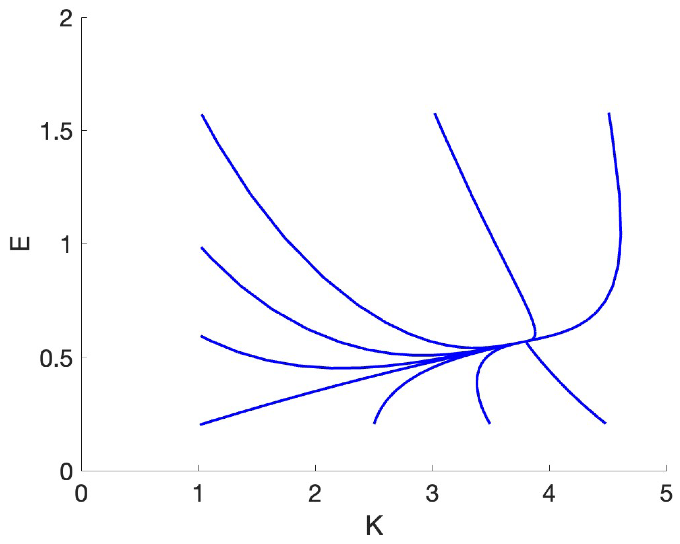
In Section 2, we will formulate a Cobb–Douglas production function Y involving the quantities K and E. The elasticity parameters $\alpha ,\beta$ and decay parameters ${\delta }_k,{\delta }_r$ will represent the effectiveness of education together with the research and capital investments coefficients $s_r,s_k$. The phase-plane depicted in Figure 1 shows the dynamics of the basic model with one stable equilibrium if $0<\alpha +\beta <1$. We expect that small social and political changes will influence capital investments. This is modeled in Section 2 by a chaotic time series.

In Section 3, we assume that the government wants to control the investments in education and research to guarantee the consumption C as a fraction p of the National Product Y. Because of the long time scale of these investments, we choose a continuous control of the investment parameter $s_r$. The consequences of the choice of the fraction p are clearly illustrated in the last figure.

As discussed in [6,9,10], the effectiveness of education may vary according to policy decisions. We will discuss the surprising consequences of a small decrease in the effectiveness of education by varying the control coefficient p in Section 3. Economic growth turns out to be very sensitive to this control.

2. The Basic Capital–Education Model

We have the conservation law that National Income Y equals the sum of Consumption C and total investment in our set-up $(I_k+I_r)$:

$$Y=C+I_k+I_r.$$

(1)

So, both investments are fractions of National Income, and we can express this as

$$I_k=s_{k}Y,I_r=s_{r}Y;0\le s_k\le 1,0<\delta \le s_r\le 1.$$

(2)

We have $s_r\ge \delta$, with $\delta$ as a small positive parameter, as all mammals teach their young at least to forage. An empirical law is the law of diminishing returns, stating the observation that, in general, an extra input of capital, education and innovation produces more growth in a sub-linear way. A generalized Cobb–Douglas production function expresses this by assuming that the National Income Y is proportional to the schooling and expertise E of the workforce and physical capital K as

$$Y=E^{\alpha }{K}^{\beta },0<\alpha ,\beta <1,$$

(3)

with $\alpha ,\beta$ as the elasticity coefficients. $E^{\alpha }$ is a productivity factor dependent on the level of education and research of the population, and in its turn, it is also dependent on the investment factor $s_r$. We will use in examples typical values of the elasticity coefficients following the cross-country survey in [6]; typical values are near $\alpha =0.20,\beta =0.35$. To choose values for quantities K and E and the elasticity coefficients is not easy. Investments in buildings for education should not be mixed with capital investments. We are using the empirical data of [6]; see also the survey [13].

Of course there are many more aspects regarding the development of National Income, but we intend in this note to consider the consequences of changes in the investment in education, research and innovation. If necessary, we can add small chaotic modulations of capital investments, which produces small modulations in the time series $Y\left(t\right)$.

The amount of capital K increases by investment and decreases through wear and tear (${\delta }_k$-proportional to K). This leads to the equation

$${\displaystyle \frac{dK}{dt}}=I_k-{\delta }_{k}K,{\delta }_k>0.$$

(4)

Using Equations (2) and (3), we find

$${\displaystyle \frac{dK}{dt}}=s_k{E}^{\alpha }{K}^{\beta }-{\delta }_{k}K.$$

(5)

The parameters $s_k,{\delta }_k$ are semi-definite positive constants; it is natural that the parameters will change with time, but at least for some time, we will assume that they are constant. For the productivity factor $E^{\alpha }$, we have in a similar way the following equation:

$${\displaystyle \frac{dE}{dt}}=s_{r}Y-{\delta }_{r}E,{\delta }_r>0,$$

(6)

with ${\delta }_r$ as a positive parameter representing loss by obsolete and forgotten expertise. Using Eqations (2), (4) and (6), we find the following system:

$$\begin{array}{c}\hfill \left\{\begin{array}{cc}{\displaystyle \frac{dK}{dt}}\hfill & =s_k{E}^{\alpha }{K}^{\beta }-{\delta }_{k}K,\hfill \\ {\displaystyle \frac{dE}{dt}}\hfill & =s_r{E}^{\alpha }{K}^{\beta }-{\delta }_{r}E.\hfill \end{array}\right.\end{array}$$

(7)

If accidentally ${\delta }_k={\delta }_r$, system (7) has an invariant manifold simply described by

$$K={\displaystyle \frac{s_k}{s_r}}E.$$

(8)

However, ${\delta }_k$ and ${\delta }_r$ are not related; so, we will pay no attention to this case. We will consider the $(E, K)$ phase-plane. Apart from the trivial solution $(E, K)=(0, 0)$, we have one critical point $(E_0, K_0)$ given by

$$E_0^{\alpha }={\displaystyle \frac{{\delta }_k}{s_k}}{K}_0^{1-\beta },K_0^{\beta }={\displaystyle \frac{{\delta }_r}{s_r}}{E}_0^{1-\alpha }.$$

(9)

This equilibrium (critical point) does not exist for arbitrary parameter values if $\alpha +\beta =1$; it would not be practical to impose this relation, as the two elasticity coefficients are qualitatively very different. Such a special choice of parameters produces in a simple way the AK model that allows for perpetual exponential growth, assuming relatively large positive savings and investment rates and ${\delta }_k,{\delta }_r$ as sufficiently small; see also [14,15]. This case is called “structurally unstable” in the mathematical theory of dynamical systems. This means that the case is exceptional in the sense that small perturbations will produce large quantitative and qualitative changes (see, for the terminology, [16]).

Consider the stability of the economic equilibrium $(E_0, K_0)$. Linearizing system (7) at the critical point $(E_0, K_0)$ gives the following 2-dimensional matrix (excluding the case $\alpha +\beta =1$):

$$\left(\begin{array}{cc}(\beta -1){\delta }_k& \alpha {\displaystyle \frac{s_k}{s_r}}{\delta }_r\\ \beta {\displaystyle \frac{s_r}{s_k}}{\delta }_k& (\alpha -1){\delta }_r\end{array}\right),$$

(10)

with trace representing the divergence of the flow near the following critical point:

$$(\alpha -1){\delta }_r+(\beta -1){\delta }_k<0.$$

(11)

As the divergence is negative in the linearized system, the flow is locally contracting. We shall show that the corresponding economic equilibrium is a stable node if $\alpha +\beta <1$; see Figure 1. The parameter values are suggested by the cross-country survey of [6] with a typical investment ratio of $s_k/s_r=4:1$.

Stability analysis of the equilibrium $E_0,K_0$.

As the divergence given by Equation (11) is negative, we have for the eigenvalues ${\lambda }_1,{\lambda }_2$ of matrix (10) that ${\lambda }_1+{\lambda }_2<0$. From the characteristic equation, we have ${\lambda }_1{\lambda }_2=(1-\alpha -\beta ){\delta }_r{\delta }_k$. So, one of the eigenvalues is positive if

$$\alpha +\beta >1.$$

(12)

In this case, the equilibrium $(E_0, K_0)$ is unstable. Regarding the cross-country survey in [6], we consider these $\alpha ,\beta$ values as less realistic. If we would have $\alpha +\beta >1$, we would have the possibility of tipping points and permanent growth of the National Product.

We assume from now on that $0<\alpha +\beta <1$.

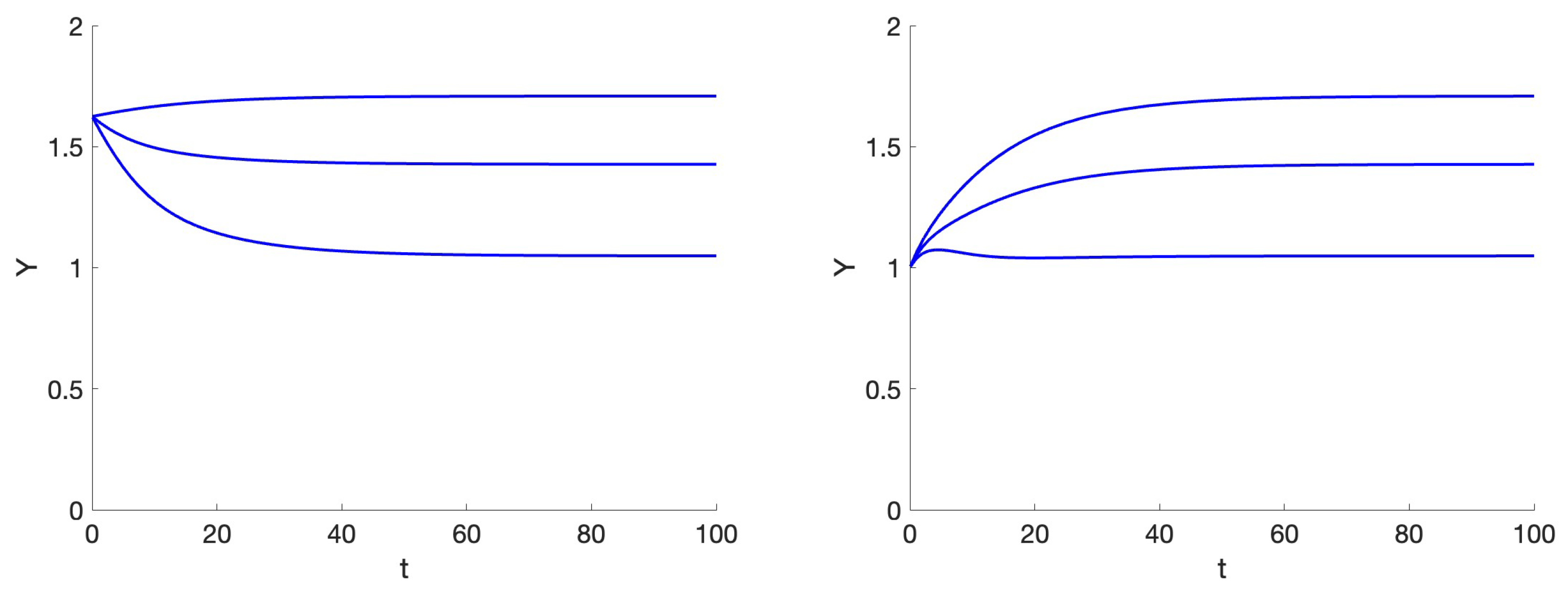
In this case, both eigenvalues ${\lambda }_1,{\lambda }_2$ are real and negative. Three typical orbits for the evolution of the National Product $Y\left(t\right)$ are shown in Figure 2. In Figure 1, it is shown that the $E,K$ phase-orbits tend to a stable equilibrium; so as expected, the National Product $Y\left(t\right)$ stabilizes at a definite value. We use the parameters of Figure 1 in Figure 2 except for different values of investment coefficient $s_r$. The lowest growth of the National Product $Y\left(t\right)$ takes place at $s_r=0.05$, slightly better for $s_r=0.1$, and again increases if $s_r=0.15$. Starting with an equal initial ratio $K/E$ produces a remarkable growth of $Y\left(t\right)$, as shown in Figure 2 (right).

2.1. The Effectiveness of Education

As discussed in [9,10,13] and in numerous newspaper articles, the investments in and the quality of education and research play an important part in economic growth. Regarding ‘quality’, we include communication tools (languages), mathematics, up-to-date tools from information theory and other modern topics, as well as specialized professional training by academic institutes and polytechnics. The ability to apply these tools in real-life situations is also essential.

An aspect of the discussion in more developed countries is also the part-time work of highly qualified workers. Especially in teaching and medical professions, the number of part-timers in developed countries has increased considerably. This leads clearly to less effectiveness, as the cost to educate and professionalize a person remains the same regardless of the number of hours worked when professionally active.

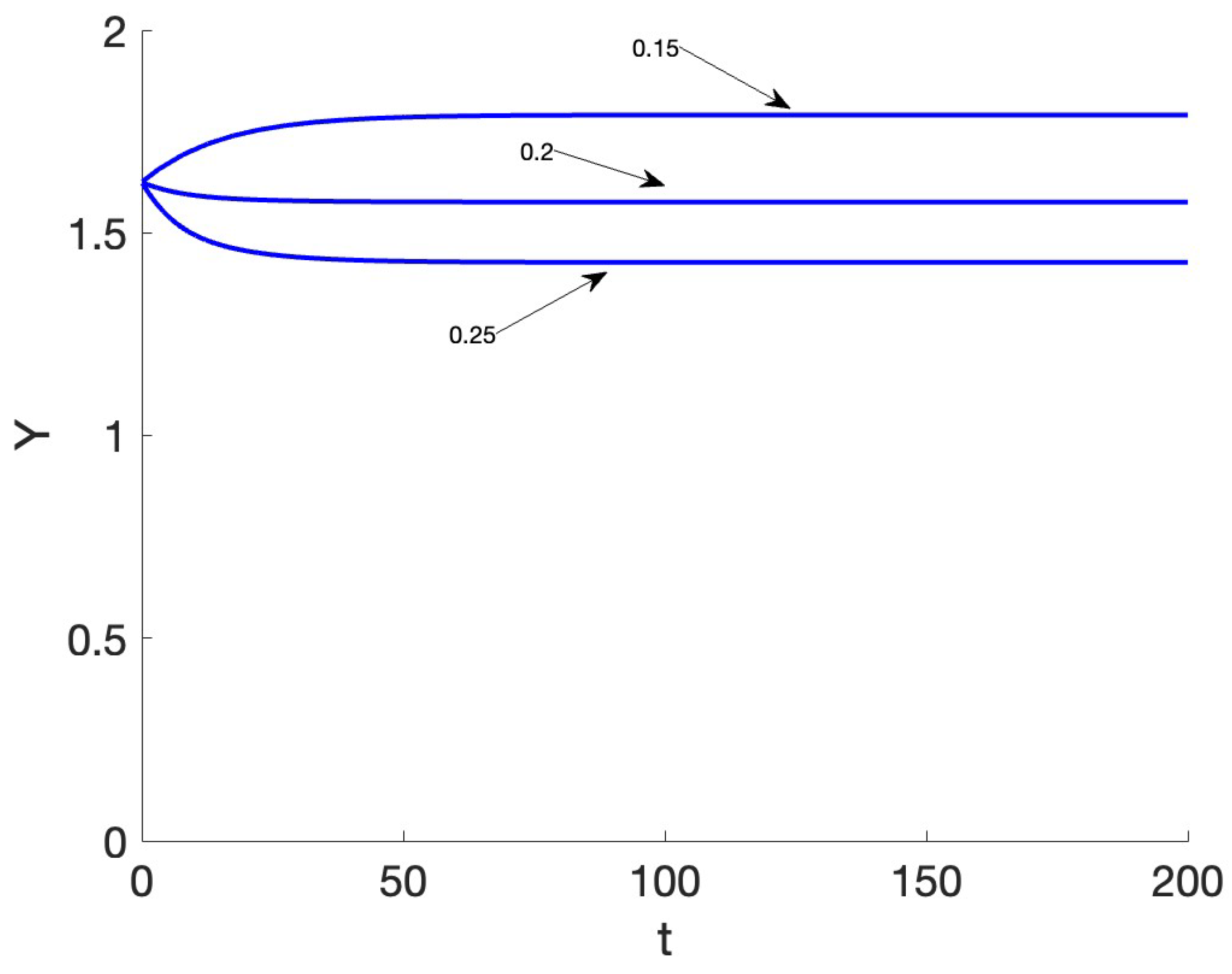
In Figure 3, we show the results of more effective education by varying ${\delta }_r$. Increasing ${\delta }_r$ means that the results of education are sooner forgotten or sooner out-of-date. One could also use the elasticity coefficient $\alpha$, but then, because of the fractal exponent near zero and possibly small or in some models negligible values of E, one has still to choose the other parameters such that initially $dY/d\alpha >0$; with the choice of ${\delta }_r$, the growth of $Y\left(t\right)$ is guaranteed when decreasing ${\delta }_r$ with fixed $\alpha$.

The lowest growth curve in Figure 3 is taken from Figure 2; decreasing ${\delta }_r$ produces more growth $Y\left(t\right)$. Methods to improve the effectivity of education are a topic of permanent discussion among teachers and educationalists. The following National Product values were obtained after 200 time steps when varying $d_r$ and keeping the other parameters as in Figure 3:

$$\begin{array}{ccccccc}{d}_r& 0.25& 0.23& 0.21& 0.19& 0.17& 0.15\\ Y& 1.43& 1.48& 1.54& 1.61& 1.68& 1.79\end{array}$$

(13)

Increasing the effectivity of education has serious consequences for economic growth.

2.2. Chaotic Fluctuations in Investments

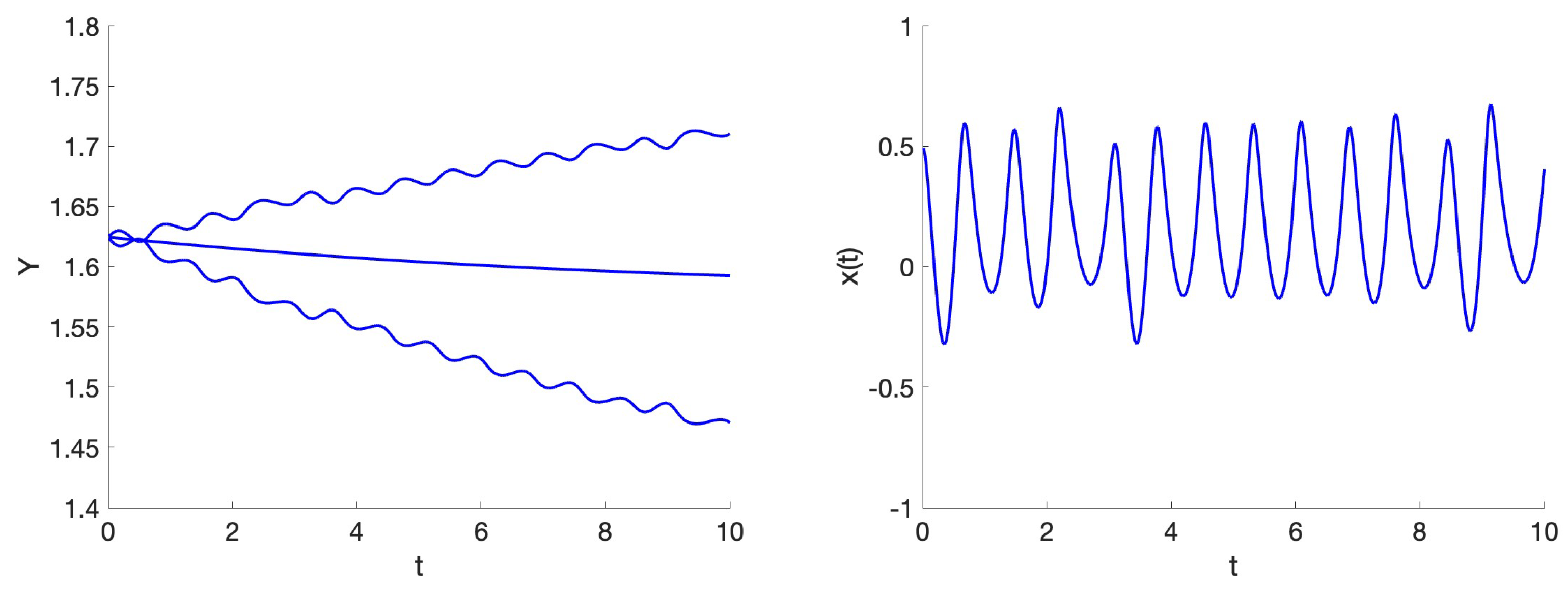
In an economy, capital investments are not fixed but are changing daily as a consequence of economic and political changes. Assuming we want to model small fluctuations that take place when there are no exceptionally large changes in the economy, we modify system (7) by replacing the capital investment coefficient $s_k$ by $s_k+cx\left(t\right)$. As an example, the time series $x\left(t\right)$ is chosen from the chaotic system NE9 studied in [17]. This system has the advantage that chaos is produced as the end product of a series of solutions with increasing periods; we still find in the chaotic motion some cyclic behaviour. In chaotic systems that arise at unstable global motion, like in the Lorenz attractor, the time series is less suitable for economic models. We modify system (7) to

$$\begin{array}{c}\hfill \left\{\begin{array}{cc}{\displaystyle \frac{dK}{dt}}\hfill & =(s_k+cx\left(t\right))E^{\alpha }{K}^{\beta }-{\delta }_{k}K,\hfill \\ {\displaystyle \frac{dE}{dt}}\hfill & =s_r{E}^{\alpha }{K}^{\beta }-{\delta }_{r}E.\hfill \end{array}\right.\end{array}$$

(14)

For reference, we present the following equations governing the chaotic system NE9:

$$\dot{x}=y,\dot{y}=-x-yz,\dot{z}=-xz+7x^2-0.55.$$

(15)

We put initially $x\left(0\right)=0.5$, $y\left(0\right)=z\left(0\right)=0$. Replacing the number $0.55$ in system (15) by other positive numbers will produce very different dynamics. The average of $x\left(t\right)$ of the NE9 system over time zero to t is of a generalized form, as $x\left(t\right)$ is not periodic or quasi-periodic. We put for the average if $t>0$:

$$A\left(t\right)={\displaystyle \frac{1}{t}}{\int }_0^{t}x\left(s\right)ds.$$

(16)

We have that the average $A\left(100\right)$ is a small positive number close to $0.14$; so, $x\left(t\right)$ spends more time at positive values than at negative investment values. We compare two growth scenarios by choosing $c=\pm 0.5$. The plus sign describes a case where a hype cycle of new technical developments produces chaotically new investments. The minus sign refers to a case where erratic political measures entail uncertainty to invest. As the time scale of investments is larger than the time fluctuations, we scale time for the fluctuations with a factor of 10.

In Figure 4, we show growth to a stable National Product Y by the case $s_k=0.4, c=0$, as well as the two cases with unpredictable chaotic oscillations.

3. Controlling Consumption

We will investigate the consequences of changes in investments in education and research by government control.

In 1961, E. Phelps [2] looked for conditions to obtain a fixed economic output to a fixed capital input ratio (the “Golden Rule”). An equilibrium solution can be obtained by suitable choices of all the parameters of a classical Cobb–Douglas function leading to so-called golden-age growth with the ratio of the National Product and capital investments constant with time. In the “Golden Rule”, model education and innovation investments are not seen as a separate type of investment, and stability questions still have to be solved at this stage.

As we will see, aiming at an optimal savings rate that maximizes per capita consumption in the long-run equilibrium is different from a direct control choosing a politically accepted consumption target as part of the increasing or decreasing National Product.

Suppose that, in a new approach, the government wants to guarantee consumption by controlling investment in education and research. There may be various reasons for this, for instance the financing of pensions of an aging population, the increase in the expenses of medical care or defense or simply a negative populist view of education as an elite activity in general. So, for political reasons, one aims then at consumption C as a certain fraction p of the national product Y. A given target of consumption C can be achieved by varying the investment factor $s_r$ with time, keeping capital investment factor $s_k$ constant. This results in the following equation to control investments:

$${\displaystyle \frac{d{s}_r}{dt}}=C-pY.$$

(17)

If the consumption C is larger than target $pY$, the investment coefficient $s_r$ for education and research has room to increase; if the consumption C is smaller than target $pY$, then $s_r$ has to decrease. This type of control is inspired by chemical physics; for references and other mathematical physics applications, see [18].

As $C=(1-s_k-s_r)Y$, we have with Equations (3)–(17) and system (7) the following 3-dimensional system:

$$\begin{array}{c}\hfill \left\{\begin{array}{cc}{\displaystyle \frac{dK}{dt}}\hfill & =s_k{E}^{\alpha }{K}^{\beta }-{\delta }_{k}K,\hfill \\ {\displaystyle \frac{dE}{dt}}\hfill & =s_r{E}^{\alpha }{K}^{\beta }-{\delta }_{r}E,\hfill \\ {\displaystyle \frac{d{s}_r}{dt}}\hfill & =(1-s_k-s_r-p)E^{\alpha }{K}^{\beta }.\hfill \end{array}\right.\end{array}$$

(18)

The equilibrium (critical point) given by (9) will change, as $s_r$ is varying by changing parameter p and the evolution of the economy; $E_0, K_0$ are again given by Equation (9) and

$$s_r=1-s_k-p.$$

(19)

Linearization at the equilibrium produces the following matrix:

$$\left(\begin{array}{ccc}(\beta -1){\delta }_k& \alpha {\displaystyle \frac{s_k}{s_r}}{\delta }_r& 0\\ \beta {\displaystyle \frac{s_r}{s_k}}{\delta }_k& (\alpha -1){\delta }_r& E_0^{\alpha }{K}_0^{\beta }\\ 0& 0& -E_0^{\alpha }{K}_0^{\beta }\end{array}\right)$$

(20)

where $s_r$ satisfies Equation (19). The characteristic equation has the same first two eigenvalues as for system (18) with $s_r$ given by Equation (19), but as a third eigenvalue ${\lambda }_3=-E_0^{\alpha }{K}_0^{\beta }$. So, the controlled equilibrium is also stable.

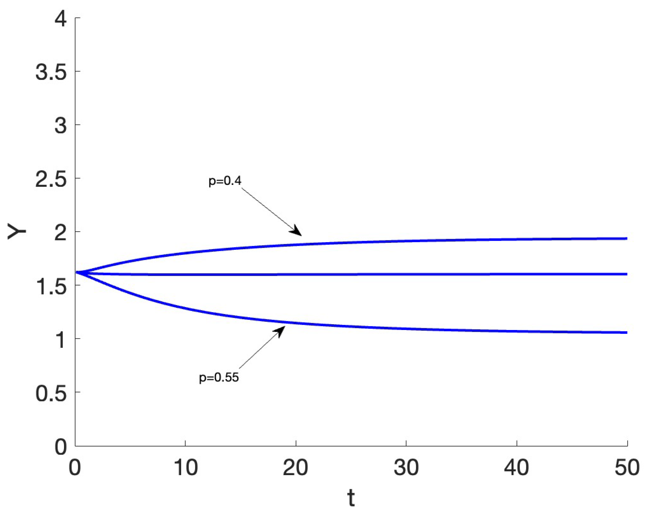
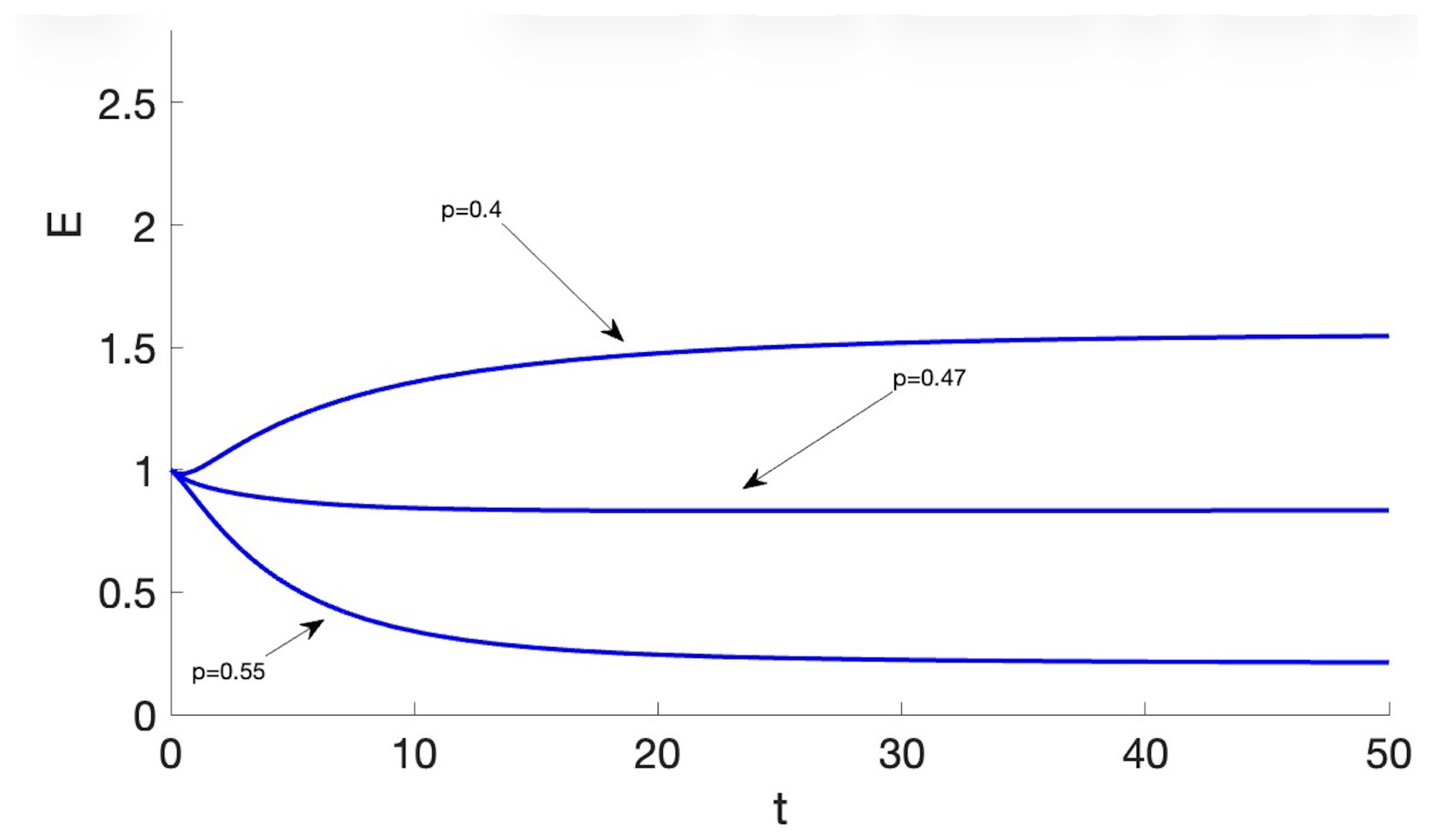
In Figure 5, we show the growth of the National Product $Y\left(t\right)$ for the cases $p=0.4, 0.47, 0.55$. We show the evolution of $E\left(t\right)$ in the corresponding three cases of p in Figure 6. We conclude that reducing the investment in education and research to increase the possibility of increasing consumption may affect economic growth negatively. A tipping point for the National Product with the parameters of Figure 5 is close to $p=0.47$. $Y\left(t\right)$ remains in this case near the starting value $1.62$ and consumption $C\left(t\right)\to 0.76$. If $p=0.55$, we have that $Y\left(t\right)\to 1.2$ and $C\left(t\right)\to 0.66$; so, trying a control aiming at higher consumption as part of the National Product may in fact reduce consumption. If $p=0.4$, we have that $Y\left(t\right)\to 1.95$ and $C\left(t\right)\to 0.78$.

4. Discussion and Conclusions

Our models are based on assumptions using conservation laws and empirical rules. A standard issue of deterministic mathematical models is that the conclusions are consequences of the assumptions made when constructing the models. However, the complexity of the relations between the assumptions and the resulting dynamics can make the results unexpected and important. For instance, in the basic model of Section 2, we have a stable equilibrium if the elasticity coefficients $\alpha , \beta$ satisfy the relation $0<\alpha +\beta <1$. Another example is the emergence of a tipping point for economic growth if the quality of education and research decreases below a certain value. Low-dimensional models may appear less realistic than models with hundreds of variables, but the calculations produce results like tipping points that change the overall picture drastically.

The results can be summarized as follows:

• We have constructed a low-dimensional macro-economic model involving the usual capital investments but with separate investments in education and research in Section 2. The basic model is modified in Section 3 by adding a control to fix consumption as a given fraction p of National Income. The control is effective and has long-term consequences for investments in education and research and, subsequently, an increase or decrease in the National Product and consumption.
• The time scales involved need careful handling. Usually economic planning covers at most a few years, but other time scales play a role. Changing, for example, taxation has direct consequences in time, while investments in education take many years to show good or bad results; on the other hand, hyping certain products and techniques or certain mood changes with regards to equities and bonds usually take place in cycles of weeks or months.
• It turns out, as shown in Section 2, that economic growth is also sensitive to the quality of education (learning something that matters and remaining well-informed) and innovation (high quality and up-to-date research). This result was obtained by small changes in the coefficient ${\delta }_r$, describing the persistence of useful knowledge and expertise, while keeping all the other parameter values constant.
• We model fluctuating sources of capital investments by introducing a chaotic modulation of the investment factor $s_k$ with hype-induced investments and the corresponding growth of National Product Y. This also includes erratic policies leading to changing investments. To study the growth and decline of the economy, it would be useful to have examples of realistic time series of such fluctuations.
• An interesting result of Section 3 is that aiming at a lower fraction $pY$ of National Product $Y\left(t\right)$ and so relatively less consumption can result in high growth and in more real consumption. We found a few tipping points describing the growth or decline of the National Product.