The Algebra of Chebyshev Polynomials and the Transfer-Matrix Approach for the One-Dimensional Ising Model with a Defect

Abstract

We investigate a random field of mutually dependent random variables (“spins”), indexed by a finite one-dimensional lattice, called in physical sciences the one-dimensional Ising model, in which the random variables can take only ±1 values (see the text for a precise definition). One of the couplings, termed a “bond,” that describes the mutual influence of two adjacent random variables is altered—it does not equal the others, thereby introducing a single “defect” bond. This defect bond represents a localised perturbation within an otherwise uniform system. Utilising the recurrence relations of Chebyshev polynomials and the bijective map between the number of spins and the polynomial index, we present a new method for calculations and systematically explore, using it, the system’s properties across different chain lengths and boundary conditions. As an application, we derive analytical expressions for the dependence of the average values of the random variables on their position within the chain, which we refer to as the “local magnetisation profile”. From the findings related to the system with a defect bond, we present a novel result for this profile under free (Dirichlet) boundary conditions and re-derive the corresponding result for antiperiodic boundary conditions.

1. Introduction

The one-dimensional Ising model occupies a central place in statistical physics, primarily due to its analytical tractability and its capacity to illustrate fundamental aspects of cooperative behaviour and phase transitions (at $T=0$) in many-body systems. Beyond the extensively used transfer matrix method [1,2], numerous alternative analytical and numerical methodologies have been considered [3,4,5,6,7,8,9,10,11], further substantiating the model’s significance as a benchmark for theoretical investigations—despite its simplicity. This is especially true when studying the finite-size model under various boundary conditions. The most commonly studied cases are those with periodic and free (Dirichlet) boundary conditions. A suitable selection of references for the latter case is represented by the works [5,12,13,14,15,16,17]. Recent studies of correlation functions can be found in [18,19].

It is worth noting some disparity in the terminology used in the literature. In their seminal monograph, McCoy and Wu [1] use the term ‘free boundary conditions’ to refer to boundary spins that are unconstrained. Alternatively, the name open boundary conditions is also often used, as well as Dirichlet boundary conditions, in the connotation of mathematical analysis.

Let us mention that the finite-size one-dimensional Ising model exemplifies the considerable increase in mathematical complexity that arises when transitioning from the thermodynamic, i.e., infinite limit system, to systems of finite size—particularly in the rigorous analysis of correlation functions (see, e.g., Equation (3.4) and Equation (3.12) in [1]). It is, furthermore, worth noting that the study of finite-size effects and the influence of boundary conditions provides a crucial conceptual bridge between idealised theoretical models and realistic, experimentally attainable one-dimensional systems.

The present study reaffirms the status of the one-dimensional Ising model as a paradigmatic system for the deployment and illustration a of complicated and structurally insightful mathematical techniques.

The method we propose, which utilises the properties of Chebyshev polynomials, offers distinct advantages, particularly in analysing the effects of different boundary conditions in finite-sized systems in conjunction with the presence of the term $h\in \mathbb{R}$, called in physical sciences a “magnetic field”, linearly coupled to the sum of $N\in {\mathbb{N}}^{+}$ random variables ${\sigma }_1,\dots ,{\sigma }_N$. Effects due to the finite number of random variables, or, more generally of “finite-size effects”, and the influence of boundary conditions, are naturally encoded in the structure of the corresponding Chebyshev polynomials, making the approach particularly well suited for the analysis of finite, i.e., non-thermodynamic-limit, systems.

This article presents two types of results, discussed in Section 2, Section 3, Section 4 and Section 5, Section 6, Section 7, Section 8, respectively. Section 2, Section 3 and Section 4 revisit, in a streamlined manner, selected known results that serve as an introduction to the proposed method and illustrate its compactness and efficiency. By contrast, Section 5, Section 6, Section 7 and Section 8 present new results concerning the properties of a more complex version of the model, namely the case with a defective bond. The main findings are summarised in the Conclusion, whereas Appendix A provides a complete list of the recurrence relations among Chebyshev polynomials referenced in the main text.

2. One Dimensional Ising Model

We consider a finite chain of length $L=aN$ (a is the lattice spacing) with $N\in \mathbb{N}$ sites labelled by $i=1,\dots ,N$ and bonds $(i,i+1)$. At each site “i” there is a discrete random variable, called spin in physical science, taking two values ${\sigma }_i=\pm 1$. The system has a nearest-neighbour interaction J and an external magnetic field H. The probability of each configuration $\sigma =\{{\sigma }_i\mid i=1,\dots ,N\}\in {\{-1,1\}}^N$ depends on a parameter which is linearly coupled to the sum of the random variables. In the physical sciences it is called the external field h. The mutual probability distribution of the random variables in $\mathit{\sigma }$ is

$${\mathbb{P}}_{\mathbb{N}}\left(\mathit{\sigma }\right)={\displaystyle \frac{\exp \{-\beta {\mathcal{H}}_N\left(\mathit{\sigma }\right)\}}{Z_N(K,h)}},$$

(1)

where

$$\beta {\mathcal{H}}_N\left(\mathit{\sigma }\right)=-K\sum _{i=1}^{N-1}{\sigma }_i{\sigma }_{i+1}-K_{BC}{\sigma }_N{\sigma }_1+h\sum _{i=1}^N{\sigma }_i,$$

(2)

and

$$Z_{\mathrm{N}}(K,h)=\sum _{\mathit{\sigma }}\exp (-\beta {\mathcal{H}}_N\left(\mathit{\sigma }\right)),$$

(3)

with the sum running over all $2^N$ configurations $\mathit{\sigma }$. The quantity ${\mathcal{H}}_N$ is the energy of the configuration $\mathit{\sigma }$ and is sometimes also called the Hamilton of the discrete system, while $Z_N$ is termed the partition function.

The term $K_{BC}{\sigma }_N{\sigma }_1$ provides the mutual influence of the boundary random variables (spins) ${\sigma }_1$ and ${\sigma }_N$ and determines the so-called boundary conditions imposed on the system. One normally considers the following: $K_{BC}=K$ (periodic, PBC); $K_{BC}=-K$ (antiperiodic, ABC); and $K_{BC}=0$ (free boundary, FB). And we use the following dimensionless quantities: $K=\beta J\ge 0$ and $h=\beta H\in \mathbb{R}$, where $\beta =1/k_{B}T$ is the inverse temperature T ($k_B$ is the Boltzmann’s constant).

Different expectation values, e.g., $\langle {\sigma }_i\rangle$ which is called the site magnetisation (or correlation functions), are computed with respect to this distribution ${\mathbb{P}}_{\mathbb{N}}\left(\mathit{\sigma }\right)$, namely

$$\langle {\sigma }_i\rangle =\sum _{\mathit{\sigma }}{\sigma }_i{\mathbb{P}}_{\mathbb{N}}\left(\mathit{\sigma }\right).$$

(4)

For simplicity, we adopt a slight abuse of notation by omitting the explicit dependence on the boundary conditions in the formulas above; these dependencies will be made explicit wherever necessary below.

From the perspective of computation, the central observation is that the partition function can be formulated as a suitable power of the transfer matrix

$$\mathbf{T}=\left(\begin{array}{cc}{e}^{K+h}& e^{-K}\\ e^{-K}& e^{K-h}\end{array}\right),$$

(5)

namely the partition function. In the case of periodic boundary conditions (PBCs), the partition function can be written as the trace of the N-th power of the transfer matrix $\mathbf{T}$,

$$Z_{\mathrm{N}}^{\left(\mathrm{periodic}\right)}(K,h)=\mathrm{Tr} \left({\mathbf{T}}^N\right).$$

The standard approach to evaluating this expression is to perform a change of basis in which the transfer matrix becomes diagonal and to determine its eigenvalues by solving the associated equation. Difficulties arise, however, when the trace operator involves products of non-commuting matrices raised to different powers. The approach developed in the current article renders such cases considerably more tractable.

3. Chebyshev Polynomials and the Transfer Matrix Approach

In this section, we summarise some the properties of the Chebyshev polynomials of the first and second kinds, $T_N\left(x\right)$ and $U_N\left(x\right)$, respectively, which are polynomials of degree N of some variable x. The definitions needed and all necessary recurrence relations, connecting Chebyshev polynomials with different indices, are collected, for a convenience of the reader, in Appendix A.

3.1. On the Use of Chebyshev Polynomials in Mathematical Physics

An approach, based on Chebyshev polynomials, arises naturally and systematically in a wide class of problems in mathematical physics, particularly in the study of superlattices, photonic crystals, and more general stratified media. The use of these polynomials in such contexts originates with the works of Abelès [20] and Jones [21], and their subsequent applications in transfer-matrix and wave-propagation problems are documented in [22,23,24], as well as in standard references [25] (§ 1.5.1, p. 69), [26] (§ 1.6.2, p. 55), and in comprehensive reviews [27,28]. One of the defining features of this approach is that finite-size effects, together with intrinsic structural periodicity, play a central role and must be treated explicitly in any consistent theoretical formulation. More recently, this approach has proven effective for other periodic systems, notably for studding some quantities in the one-dimensional Ising model under periodic, antiperiodic and Dirichlet boundary conditions [29,30,31]. It is important to present a systematic, but simple, formulation of the concept necessary for using the Chebyshev polynomials in the statistical mechanics of one-dimensional Ising systems for studding more complicated cases, or quantities.

3.2. Key Properties of the Transfer Matrix

It is convenient to work with the unimodular transfer matrix $\tilde{\mathbf{T}}$ associated with the one-dimensional Ising model in an external magnetic field h, and with dimensionless inverse temperature $K=\beta J$

$$\tilde{\mathbf{T}}=\left(\begin{array}{cc}{\displaystyle \frac{e^{K+h}}{r}}& {\displaystyle \frac{e^{-K}}{r}}\\ {\displaystyle \frac{e^{-K}}{r}}& {\displaystyle \frac{e^{K-h}}{r}}\end{array}\right), det\left(\tilde{\mathbf{T}}\right)=1, \mathrm{Tr}\left(\tilde{\mathbf{T}}\right)=2{\displaystyle \frac{e^K\cosh \left(h\right)}{r}}.$$

(6)

Here the normalisation factor r is chosen to ensure unimodularity:

$$r=\sqrt{2\sinh \left(2K\right)}.$$

(7)

The eigenvalues ${\lambda }_{\pm }$ of $\tilde{\mathbf{T}}$ are

$${\lambda }_{\pm }=a\pm \sqrt{a^2-1}, a=\frac{1}{2}\mathrm{Tr}\left(\tilde{\mathbf{T}}\right)={\displaystyle \frac{e^K\cosh \left(h\right)}{r}}.$$

(8)

Remark 1.

In the one-dimensional Ising model, the dimensionless transfer-matrix parameter

$$a(K,h)={\displaystyle \frac{e^K\cosh \left(h\right)}{\sqrt{2\sinh \left(2K\right)}}}, K=\beta J, h=\beta H,$$

(9)

plays a crucial role. Indeed, the entire dependence of the partition function on the model parameters is encoded in a degree-N polynomial whose single argument is a. Having in mind that the correlation length ξ is determined via the eigenvalue ratio ${\lambda }_{+}/{\lambda }_{-}$, see, e.g., [2],

$${\xi }^{-1}(K,h)=\ln \left[{\displaystyle \frac{{\lambda }_{+}(K,h)}{{\lambda }_{-}(K,h)}}\right]=\ln \left[{\displaystyle \frac{a(K,H)+\sqrt{a{(K,h)}^2-1}}{a(K,h)-\sqrt{a{(K,h)}^2-1}}}\right],$$

(10)

and solving for a in terms of ξ, one obtains

$$a(K,h)=\cosh \left({\displaystyle \frac{1}{2\xi (K,h)}}\right).$$

(11)

Henceforth, to simplify the notation, we suppress the arguments h and K whenever no ambiguity arises. According to Equation (9), when $K\gg 1$ one derives $a\to \cosh h>1$. If, in addition, $h\to 0$, one has $a\to 1$, which implies $\xi \to \infty$. Thus, for any $N\gg 1$ it is possible to have both $N\gg \xi$ as well as $N\simeq \xi$.

As follows from Equation (6), the standard (non-normalized) transfer matrix $\mathbf{T}$ can be expressed in terms of $\tilde{\mathbf{T}}$ as

$$\mathbf{T}=r \tilde{\mathbf{T}}=\sqrt{2\sinh \left(2K\right)} \tilde{\mathbf{T}}; \mathrm{obviously} r=det\left(\mathbf{T}\right).$$

(12)

Our analysis is based on a structural result from the theory of the group $SL(2,\mathbb{R})$, which plays a central role in the transfer-matrix formulation of the one-dimensional Ising model. We formulate this result in the form of Lemma 1 and provide a transparent proof that elucidates the structure of real $2\times 2$ matrices and their fundamental connection with Chebyshev polynomials, as naturally realized by the Ising transfer matrix.

Lemma 1.

Let $\tilde{\mathbf{T}}$ be defined as in Equation (6), and set

$$a:={\displaystyle \frac{1}{2}}\mathrm{Tr}\left(\tilde{\mathbf{T}}\right).$$

Then, for all integers $N\ge 1$, its powers satisfy

$${\tilde{\mathbf{T}}}^N=U_{N-1}\left(a\right) \tilde{\mathbf{T}}-U_{N-2}\left(a\right) \mathbf{I},$$

(13)

where $U_n\left(a\right)$ is the Chebyshev polynomial of the second kind.

Proof. 

The characteristic polynomial of $\tilde{\mathbf{T}}$ is

$$r^2-2ar+1=0,$$

with distinct roots $r_1\ne r_2$. By the Cayley–Hamilton theorem,

$${\tilde{\mathbf{T}}}^2-2a \tilde{\mathbf{T}}+\mathbf{I}=0,$$

which immediately gives the second-order matrix recurrence relation

$${\tilde{\mathbf{T}}}^N=2a {\tilde{\mathbf{T}}}^{ N-1}-{\tilde{\mathbf{T}}}^{ N-2}, N\ge 2.$$

This recurrence relation is formally identical to that satisfied by the Chebyshev polynomials of the second kind, providing the rigorous mathematical foundation of Lemma 1: the powers of $\tilde{\mathbf{T}}$ can be expressed linearly in terms of $U_{N-1}\left(a\right)$ and $U_{N-2}\left(a\right)$.

The solution of this recurrence relation is

$${\tilde{\mathbf{T}}}^N=\mathbf{A} r_1^N+\mathbf{B} r_2^N,$$

with

$$\mathbf{A}={\displaystyle \frac{\tilde{\mathbf{T}}-r_2\mathbf{I}}{r_1-r_2}}, \mathrm{and} \mathbf{B}={\displaystyle \frac{r_1\mathbf{I}-\tilde{\mathbf{T}}}{r_1-r_2}}.$$

Using the Binet formula for Chebyshev polynomials of the second kind,

$$U_{N-1}\left(a\right)={\displaystyle \frac{r_1^N-r_2^N}{r_1-r_2}}, \mathrm{and} U_{N-2}\left(a\right)={\displaystyle \frac{r_1^{N-1}-r_2^{N-1}}{r_1-r_2}},$$

we solve for $r_1^N$ and $r_2^N$ and substitute into the above solution, which yields

$${\tilde{\mathbf{T}}}^N=U_{N-1}\left(a\right) \tilde{\mathbf{T}}-U_{N-2}\left(a\right) \mathbf{I}.$$

This completes the proof. □

In the physical context of the one-dimensional Ising model, consider a segment of length p, represented by the transfer matrix $\tilde{\mathbf{T}}$, while the remainder of the chain of length $N-p-1$ is represented by the matrix $\tilde{\mathbf{L}}$. Lemma 1 shows that the powers of $\tilde{\mathbf{T}}$ remain closed within the two-dimensional linear algebra spanned by $\mathbf{I}$ and $\tilde{\mathbf{T}}$, so that

$${\tilde{\mathbf{T}}}^p=U_{p-1}\left(a\right) \tilde{\mathbf{T}}-U_{p-2}\left(a\right) \mathbf{I}.$$

Consequently, traces of products of such segments, for example

$$\mathrm{Tr}\left({\tilde{\mathbf{T}}}^p{\tilde{\mathbf{L}}}^{ N-p-1}\right),$$

can be evaluated directly, reducing the computation to the multiplication of two $2\times 2$ matrices, without the need for unitary transformations or the diagonalization of either matrix. The representation in terms of Chebyshev polynomials ensures an elegant and efficient solution while making the dependence on segment length p explicit.

Remark 2.

Lemma 1 is purely a mathematical statement about powers of $\tilde{\mathbf{T}}$ and does not depend on the position of p along the chain. In physical applications, the integer p serves as a segment index, representing the length of a subchain. For chains with non-periodic boundary conditions, the trace generally depends on p, and the Chebyshev-polynomial form makes this dependence both explicit and computationally convenient.

Remark 3.

The sequences ${\left\{T_n\left(a\right)\right\}}_{n\in \mathbb{Z}}$ and ${\left\{U_n\left(a\right)\right\}}_{n\in \mathbb{Z}}$ are polynomials with integer coefficients, i.e., elements of the polynomial ring $\mathbb{Z}\left[a\right]$. This property reflects the underlying algebraic structure connecting the unimodular Ising transfer matrix with the recurrence relations defining the Chebyshev polynomials. In particular, it guarantees that the powers of the transfer matrix—and any derived quantities, such as the partition function, correlation functions, etc.—can be expressed in a fully exact, closed form, without introducing irrational numbers or fractions.

This integer-coefficient property highlights both the predictability and universality of the recurrence relation: the same algebraic structure applies to any $2\times 2$ unimodular matrix. Historically, a general formula for the N-th power of any unimodular matrix has been rediscovered repeatedly in the literature (see, e.g., [28]). It was derived using classical methods, most commonly via the Cayley–Hamilton theorem, or by direct mathematical induction. Our proof is simple and straightforward.

From Lemma 1, using the recurrence relation between Chebyshev polynomials of the first kind $T_N\left(z\right)$ and second kind $U_N\left(x\right)$, defined in (A5), one obtains the elegant formula

$${\displaystyle \frac{1}{2}} \mathrm{Tr}\left({\tilde{\mathbf{T}}}^N\right)=T_N\left(a\right).$$

(14)

An elementary proof of Equation (14), based on the Newton–Girard identities, was given in Ref. [32]. In the present setting, this identity establishes a direct connection between the partition function

$$Z_N^{\left(\mathrm{periodic}\right)}(K,h)=\mathrm{Tr}\left({\mathbf{T}}^N\right)=2{\left[\sqrt{2\sinh \left(2K\right)} \right]}^N{T}_N\left(a\right),$$

(15)

and the Chebyshev polynomials $T_N\left(a\right)$ [29], thereby underscoring the interplay between statistical mechanics and classical mathematics. The Chebyshev polynomials of the first kind, $T_N\left(a\right)$, are central to this framework, with the argument a explicitly depending on physical parameters such as the coupling K and external field h. Thus, they encode the spectral properties of the transfer matrix, enabling explicit calculation of thermodynamic quantities and revealing the model’s algebraic structure and characteristic behaviour.

4. Chebyshev and Lucas Polynomial Algebras in the One-Dimensional Ising Model

Recently, it has been demonstrated that the emergence of Chebyshev polynomials—either of the first kind, $T_n\left(x\right)$, or of the second kind, $U_n\left(x\right)$—provides a powerful and systematic computational framework. Their appearance is closely tied to the choice of finite-size boundary conditions imposed on the model, as discussed in Refs. [29,30,31]. This correspondence highlights the effective role of underlying recurrence relations, which naturally encode both the finite-size geometry and the associated boundary constraints. The existence of polynomials defined by second-order linear recurrence relations in the one-dimensional Ising model is, of course, not a new observation. The effective use of generalised Fibonacci and Lucas polynomials in this context has already been reported in [8,33,34]. This naturally leads to an exploration of whether the Lucas or Chebyshev polynomials might be more suitable for the analysis. The answer is most likely determined by the relationship that exists between these two families of polynomials.

The Lucas polynomials satisfy the recurrence relation

$$L_n\left(x\right)=x{L}_{n-1}\left(x\right)+L_{n-2}\left(x\right),$$

(16)

where $n\ge 2$, with $L_0\left(x\right)=2$ and $L_1\left(x\right)=x$.

The Chebyshev polynomials of the first and second kinds, $T_n\left(x\right)$ and $U_n\left(x\right)$, satisfy the common recurrence relation (see, Appendix A)

$$C_n\left(x\right)=2x C_{n-1}\left(x\right)-C_{n-2}\left(x\right), n\ge 2,$$

(17)

with arbitrary initial conditions $C_0\left(x\right)$ and $C_1\left(x\right)$. The choice $C_0\left(x\right)=1$ and $C_1\left(x\right)=x$ yields $C_n\left(x\right)=T_n\left(x\right)$, whereas $C_0\left(x\right)=1$ and $C_1\left(x\right)=2x$ yields $C_n\left(x\right)=U_n\left(x\right)$. Even for the Chebyshev polynomials, the literature introduces a special convention to remove powers of two in the explicit formulas for $T_n\left(x\right)$ and $U_n\left(x\right)$, as these powers are cumbersome in analytical calculations; see [35,36].

Specifically, for the Chebyshev polynomials of the first kind $T_n\left(x\right)$, the relation reads as follows:

$$2T_n\left({\displaystyle \frac{x}{2}}\right)=i L_n(-ix), x\in \mathbb{C}, n\ge 0.$$

(18)

The situation, however, differs for the second-kind Chebyshev polynomials $U_n\left(x\right)$, which provide a minimal, canonical basis for representing powers of the transfer matrix across all boundary conditions. By applying the recurrence relations for Chebyshev polynomials Equation (A7) in conjunction with Equation (18), one obtains the following identity:

$$U_n\left({\displaystyle \frac{x}{2}}\right)-U_{n-2}\left({\displaystyle \frac{x}{2}}\right)=i L_n(-ix), x\in \mathbb{C}, n\ge 0.$$

For comprehensive bibliographical comments on the links between Chebyshev polynomials and other well-studied polynomial families, such as the Lucas polynomials, see Ref. [37].

To further demonstrate the utility of our Chebyshev polynomial-based method, we consider in the next section some analytically more involved cases.

5. Partition Function of One-Dimensional Ising Chain with a Defect Bond

Definition 1.

The one-dimensional Ising model with a defect bond is defined as a spin system on a ring of N sites, with spin variables ${\sigma }_i\in \{-1,+1\}$, $i=1,\dots ,N$, subject to periodic boundary conditions. Nearest-neighbour interactions are uniform with coupling constant K, except for a single bond of strength $K_a$ that breaks translational invariance. The energy of a spin configuration $\mathit{\sigma }=({\sigma }_1,\dots ,{\sigma }_N)$ is given by

$$-\beta {\mathcal{H}}_N\left(\mathit{\sigma }\right)=K_a {\sigma }_1{\sigma }_2+K\sum _{i=2}^{N-1}{\sigma }_i{\sigma }_{i+1}+K_a {\sigma }_N{\sigma }_1+h\sum _{i=1}^N{\sigma }_i.$$

(19)

Remark 4.

The presence of the defect bond with coupling $K_a\ne K$ breaks the translational invariance of the homogeneous one-dimensional Ising chain. As a consequence, thermodynamic quantities acquire additional contributions associated with the defect, which persist in the finite-size system and may give rise to surface or interface effects. In the homogeneous limit $K_a=K$, the standard translationally invariant one-dimensional Ising model with periodic boundary conditions is recovered.

The partition function of the chain with a “defect” at a site $i=1$ obviously is as follows:

$$Z_{\mathrm{N}}^{\left(\mathrm{db}\right)}(K,h):=\sum _{{\sigma }_1,\cdots ,{\sigma }_N}{\mathbf{T}}_d({\sigma }_1,{\sigma }_2)\mathbf{T}({\sigma }_2,{\sigma }_3)\cdots \mathbf{T}({\sigma }_N,{\sigma }_1),$$

(20)

where we have introduced the $2\times 2$ standard transfer matrix $\mathbf{T}$, see Equation (5), with elements

$$\langle {\sigma }_i\left|\mathbf{T}\right|{\sigma }_j\rangle =\exp [K{\sigma }_i{\sigma }_j+{\displaystyle \frac{h}{2}}({\sigma }_i+{\sigma }_j)] \mathrm{and} \mathbf{T}=r\tilde{\mathbf{T}}.$$

(21)

The “defect” transfer matrix is given by

$${\mathbf{T}}_{\mathbf{d}}=\left(\begin{array}{cc}{e}^{K_a+h}& e^{-K_a}\\ e^{-K_a}& e^{K_a-h}\end{array}\right).$$

(22)

Recently, certain aspects of this model have been investigated using standard techniques; see Ref. [38]. In contrast, the approach adopted here offers several advantages, which are discussed below. We now proceed with the following result.

Theorem 1.

The partition function Equation (20) is given by the relation

$$Z_N^{\left(\mathrm{db}\right)}(K,K_a,h)=2r^N\left[a{e}^{K_a-K}{U}_{N-1}\left(a\right)-{\displaystyle \frac{\sinh (K+K_a)}{\sinh \left(2K\right)}}{U}_{N-2}\left(a\right)\right].$$

(23)

Proof. 

The corresponding partition function Equation (20) can be expressed as a product of $2\times 2$ matrices:

$$Z_{\mathrm{N}}^{\left(\mathrm{db}\right)}(K,K_a,h):=r^{N-1}\mathrm{Tr}\left\{{\mathbf{T}}^d{\tilde{\mathbf{T}}}^{(N-1)}\right\}.$$

(24)

By using the following relation (which follows from Lemma 1):

$${\mathbf{T}}_d{\tilde{\mathbf{T}}}^{N-1}=U_{N-2}\left(a\right) {\mathbf{T}}_{\mathbf{d}}\tilde{\mathbf{T}}-U_{N-3}\left(a\right) {\mathbf{T}}_{\mathbf{d}}\mathbf{I},$$

(25)

we have

$$\begin{array}{c}\hfill \mathrm{Tr}\left[{\mathbf{T}}_d{\tilde{\mathbf{T}}}^{N-1}\right]=U_{N-2}\left(a\right) \mathrm{Tr}\left\{{\mathbf{T}}_d\tilde{\mathbf{T}}\right\}-U_{N-3}\left(a\right) \mathrm{Tr}\left\{{\mathbf{T}}_d\mathbf{I}\right\}.\end{array}$$

(26)

After some simple algebra we obtain

$$\begin{array}{c}\hfill \mathrm{Tr}\left\{{\mathbf{T}}_d\tilde{\mathbf{T}}\right\}={\displaystyle \frac{2}{r}}[2{\cosh }^2\left(h\right)e^{K+K_a}-2\sinh (K+K_a)]\end{array}$$

(27)

and

$$\mathrm{Tr}\left[{\mathbf{T}}_d\mathbf{I}\right]=2e^{K_a}\cosh \left(h\right).$$

(28)

Then, Equation (26), can be rewritten as

$$\mathrm{Tr}\left[{\mathbf{T}}_d{\tilde{\mathbf{T}}}^{N-1}\right]={\displaystyle \frac{4}{r}}\left[{\cosh }^2\left(h\right)e^{K+K_a}-\sinh (K+K_a)\right]U_{N-2}\left(a\right)-2e^{K_a}\cosh \left(h\right)U_{N-3}\left(a\right).$$

(29)

Now, using the definitions of quantities a and r, it is easy to obtain

$${\displaystyle \frac{1}{r}}\mathrm{Tr}\left[{\mathbf{T}}_d{\tilde{\mathbf{T}}}^{N-1}\right]=2\left\{a{e}^{K_a-K}[2a{U}_{N-2}\left(a\right)-U_{N-3}\left(a\right)]-{\displaystyle \frac{\sinh (K+K_a)}{\sinh 2K}}{U}_{N-2}\left(a\right)\right\}.$$

(30)

Finally, after using the recurrence relation (see, Equation (A3)) between Chebyshev polynomials for $U_N\left(z\right)$, explicitly

$$U_{N-1}\left(a\right)=2a{U}_{N-2}\left(a\right)-U_{N-3}\left(a\right),$$

(31)

one can transform the algebraic sum of first and third therms in Equation (30) exactly in the rhs of Equation (23), which proves the theorem. □

In [38], this result was derived through an alternative approach, without using the Chebyshev polynomial properties, which explicitly involves the eigenvalues of the transfer matrix.

Equation (23) provides an unified representation that includes, as special cases, the results corresponding to periodic $(K_a=K)$ (see Equation (15), and antiperiodic $(K_a=-K)$ boundary conditions (see Equation (3.11) in Ref. [29]), as well as the case of free (Dirichlet) boundaries $(K_a=0)$, cf. Equation (37), as derived in [30]. We now verify this statement.

Corollary 1.

Let us consider the tree boundary condition mentioned.

• For periodic boundary conditions we set $K_a=K$ in Equation (23). Immediately, using Equation (A5) we find that

  $$Z_{\mathrm{N}}^{\left(\mathrm{db}\right)}(K,h)=2r^N\left[a U_{N-1}\left(a\right)-U_{N-2}\left(a\right)\right]=2r^N{T}_N\left(a\right).$$

  (32)
  This result coincides exactly with the expression for the grand-canonical partition function under periodic boundary conditions, as given in Equation (15).
• For antiperiodic boundary conditions we set $K_a=-K$ in Equation (23). Then,

  $$\begin{array}{c}\hfill Z_{\mathrm{N}}^{\left(\mathrm{db}\right)}(K,-K,h)=2r^N{e}^{-2K}a U_{N-1}\left(a\right),\end{array}$$

  (33)
  which coincides with the known result for the grand-canonical partition function under antiperiodic boundary conditions, see Equation (3.11) in ref. [29].
• For free boundary conditions we set $K_a=0$ in Equation (23). Then, the result is as follows:

  $$Z_{\mathrm{N}}^{\left(\mathrm{db}\right)}(K,0,h)=2r^{N-1}\left[\cosh \left(h\right) U_{N-1}\left(a\right)-{\displaystyle \frac{2}{r}}\sinh \left(K\right) U_{N-2}\left(a\right)\right].$$

  (34)

Remark 5.

Since the numerous recurrence relations among Chebyshev polynomials allow the final result to be expressed in different forms depending on the chosen calculation path, we will illustrate this property by presenting several equivalent forms of the partition function in the case of free (Dirichlet) boundary conditions.

In Ref. [30], the following expression for the grand canonical partition function was obtained:

$$Z_{\mathrm{N}}^{\left(\mathrm{free}\right)}(K,h)=2r^{ N-1}\left[{\displaystyle \frac{1}{r}}\left(e^K{\sinh }^2\left(h\right)+e^{-K}\right) U_{N-2}\left(a\right)+\cosh \left(h\right) T_{N-1}\left(a\right)\right].$$

(35)

After applying the recurrence relation Equation (A5)

$$T_{N-1}\left(a\right)=a U_{N-2}\left(a\right)-U_{N-3}\left(a\right),$$

(36)

one can verify that Equation (35) is equivalent to

$$Z_{\mathrm{N}}^{\left(\mathrm{free}\right)}(K,h)=2r^{N-1}\left\{{\displaystyle \frac{1}{r}}\left(e^K\cosh \left(2h\right)+e^{-K}\right)U_{N-2}\left(a\right)-\cosh \left(h\right)U_{N-3}\left(a\right)\right\}.$$

(37)

Furthermore, applying the recurrence relation Equation (A3)

$$U_{N-1}\left(a\right)=2a{U}_{N-2}\left(a\right)-U_{N-3}\left(a\right),$$

(38)

one obtains the compact expression Equation (34).

6. Asymptotic Expansion of the Partition Function with a Defect Bond

Now we need the following preparatory proposition for the asymptotes of the Chebyshev polynomials $U_n\left(a\right)$ for $a>1$:

Proposition 1.

Recall that the Chebyshev polynomials of the second kind admit the representation (see, e.g., Refs. [35,36,39])

$$U_n\left(a\right)={\displaystyle \frac{{\lambda }_{+}^{ n+1}-{\lambda }_{-}^{ n+1}}{2\sqrt{a^2-1}}}={\displaystyle \frac{{\lambda }_{+}^{ n+1}}{2\sqrt{a^2-1}}}\left[1-{\left({\displaystyle \frac{{\lambda }_{-}}{{\lambda }_{+}}}\right)}^{n+1}\right],$$

(39)

where, for $a>1$, one has ${\lambda }_{+}>1$, while $\left|{\lambda }_{-}\right|<1$. Hence, the asymptotic behaviour of $U_n\left(a\right)$ for $n\to \infty$ is governed by the growing branch ${\lambda }_{+}$. More precisely,

$$U_n\left(a\right)\sim {\displaystyle \frac{{\lambda }_{+}^{ n+1}}{2\sqrt{a^2-1}}}, n\to \infty .$$

(40)

Theorem 2.

For $N\gg 1$, the following presentation of the partition takes place

$$Z_{\mathrm{N}}^{\left(\mathrm{db}\right)}(K,K_a,h)\sim {\left(r{\lambda }_{+}\right)}^{N}C(K,K_a)\left[1+O \left(e^{-N/\xi }\right)\right],$$

(41)

where the amplitude $C(K,K_a)$ is

$$C(K,K_a,h)\equiv \left[e^{K_a-K} {\displaystyle \frac{a}{\sqrt{a^2-1}}}-{\displaystyle \frac{\sinh (K+K_a)}{\sinh \left(2K\right)}}{\displaystyle \frac{{\lambda }_{-}}{\sqrt{a^2-1}}}\right].$$

(42)

Proof. 

From Equation (39), one finds

$$\begin{array}{cc}\hfill U_{N-1}\left(a\right)& \sim {\displaystyle \frac{{\lambda }_{+}^{ N}}{2\sqrt{a^2-1}}}\left(1-e^{-N/\xi }\right),\hfill \end{array}$$

(43)

$$\begin{array}{cc}\hfill U_{N-2}\left(a\right)& \sim {\displaystyle \frac{{\lambda }_{+}^{ N-1}}{2\sqrt{a^2-1}}}\left(1-e^{-(N-1)/\xi }\right),\hfill \end{array}$$

(44)

where the correlation length $\xi$ is given in Equation (10). Substituting these expressions into the grand-canonical partition function with a defect bond yields

$$\begin{array}{cc}\hfill Z_{\mathrm{N}}^{\left(\mathrm{db}\right)}(K,K_a,h)& \sim r^N{\lambda }_{+}^N\left[e^{K_a-K} {\displaystyle \frac{a}{\sqrt{a^2-1}}}-{\displaystyle \frac{\sinh (K+K_a)}{\sinh \left(2K\right)}}{\displaystyle \frac{{\lambda }_{-}}{\sqrt{a^2-1}}}\right]\hfill \\ \hfill & +O \left(r^N{\lambda }_{+}^{ N-1}{e}^{-N/\xi }\right),\hfill \end{array}$$

(45)

which is the statement in Equation (41). Note that $C(K,K_a,h)$ does not depend on N. □

The representation given by Equation (41) clearly separates the different contributions into the partition function based on their dependence on the system size N. This is most clearly seen in the quantity $f_N(K,K_a,h)$, called the free energy of the system in statistical physics, defined as follows:

$$\begin{array}{ccc}\hfill \beta f_N(K,K_a,h)& :=& -{\displaystyle \frac{1}{N}}\ln Z_{\mathrm{N}}^{\left(\mathrm{db}\right)}(K,K_a,h)\hfill \\ & =& f_{\mathrm{bulk}}(K,h)+{\displaystyle \frac{1}{N}}{f}_{\mathrm{surface}}^{\left(\mathrm{db}\right)}(K,K_a,h)+\Delta f_N^{\left(\mathrm{db}\right)}(K,K_a,h),\hfill \end{array}$$

(46)

where

$$f_{\mathrm{bulk}}(K,h)=\ln (r {\lambda }_{+})$$

is called the bulk free energy, independent of $K_a$ and N, while

$$f_{\mathrm{surface}}^{\left(\mathrm{db}\right)}(K,K_a,h)=-\ln C(K,K_a,h)$$

(47)

is termed surface (interface) free energy and is independent of N but dependent on $K_a$. The remaining term, $\Delta f_N^{\left(\mathrm{db}\right)}(K,K_a,h)$, contains higher-order corrections $o\left(1\right)$ that vanish as $N\to \infty$. Consequently, the manner in which $f_N(K,K_a,h)$ approaches its bulk limit as $N\to \infty$ depends crucially on the behaviour of $C(K,K_a,h)$, which is a generic feature in the presence of boundary conditions imposed on the system. At this stage, it is convenient to briefly discuss the most important values of $K_a$, corresponding to different boundary conditions.

Corollary 2.

For the periodic ($K=K_a$), antiperiodic ($K=-K_a$), and free (Dirichlet) ($K_a=0$), also known as the free or missing neighbours boundary conditions, one has, consequently, the following:

• If $K_a=K$ (periodic boundary conditions) we get

  $$C(K,K,h)=1$$

  and thus

  $$f_N^{\left(\mathrm{periodic}\right)}(K,h)=f_{\mathrm{bulk}}(K,h)+O\left(e^{-N/\xi }\right).$$

  (48)
  Therefore, $f_N^{\left(\mathrm{periodic}\right)}(K,h)$ approaches the bulk result exponentially in N.
• If $K_a=-K$ (antiperiodic boundary conditions) one has

  $$f_N^{\left(\mathrm{antiperiodic}\right)}(K,h)=f_{\mathrm{bulk}}(K,h)+{\displaystyle \frac{1}{N}}{f}_{\mathrm{surface}}^{\left(\mathrm{antiperiodic}\right)}(K,h)+O\left(e^{-N/\xi }\right),$$

  (49)

  where the antiperiodic surface free energy is

  $$\begin{array}{ccc}\hfill f_{surface}^{\left(antiperiodic\right)}(K,h)& :=& -\ln \left[C(K,-K,h)\right]=-\ln \left[{\displaystyle \frac{e^{-2K}\cosh \left(h\right)}{\sqrt{{\sinh }^2\left(h\right)+e^{-4K}}}}\right]\hfill \\ & =& 2K-\ln {\displaystyle \frac{1+{\lambda }_{-}(K,h)/{\lambda }_{+}(K,h)}{1-{\lambda }_{-}(K,h)/{\lambda }_{+}(K,h)}}\hfill \\ & =& 2K-\ln {\displaystyle \frac{1+\exp (-1/\xi (K,h\left)\right)}{1-\exp (-1/\xi (K,h\left)\right)}},\hfill \end{array}$$

  (50)

  which coincides with the result, Equation (3.9) in Ref. [29].
• If $K_a=0$ (free boundary conditions) the result is

  $$f_N^{\left(\mathrm{free}\right)}(K,h)=f_{\mathrm{bulk}}(K,h)+{\displaystyle \frac{1}{N}}{f}_{\mathrm{surface}}^{\left(\mathrm{free}\right)}(K,h)+O\left(e^{-N/\xi }\right),$$

  (51)

  where the free surface free energy is
  $$\begin{array}{ccc}\hfill f_{\mathrm{surface}}^{\left(\mathrm{free}\right)}(K,h)& :=& -\ln \left[C(K,0,h)\right]=-\ln \left\{{\displaystyle \frac{1}{2\cosh \left(K\right)}}\left[1+{\displaystyle \frac{e^{-2K}\cosh \left(h\right)}{\sqrt{{\sinh }^2\left(h\right)+e^{-4K}}}}\right]\right\}\hfill \\ & =& \ln \cosh \left(K\right)+\ln \left[1-{\lambda }_{-}(K,h)/{\lambda }_{+}(K,h)\right]\hfill \\ & =& \ln \cosh \left(K\right)+\ln \left[1-\exp (-1/\xi (K,h\left)\right)\right].\hfill \end{array}$$

  (52)
  This, after some algebraic manipulations, coincides with the well-known result of McCoy and Wu [1].

Note that expansion Equations (48), (49), and (51) make sense only if $N\gg \xi (K,h)$. When $N\simeq \xi$, we are in the realm of the finite-size scaling theory [40,41,42,43,44]. In this regime, one interesting object of study is the critical Casimir force, which is an important present-day topic for investigation. A pedagogical introduction to the finite-size scaling theory and to the critical Casimir force is given in [43]. A review of the existing exact results for this force is given in [44]. For studying it, a much more complicated theory is needed, which is out of the scope of the current article and will be considered elsewhere.

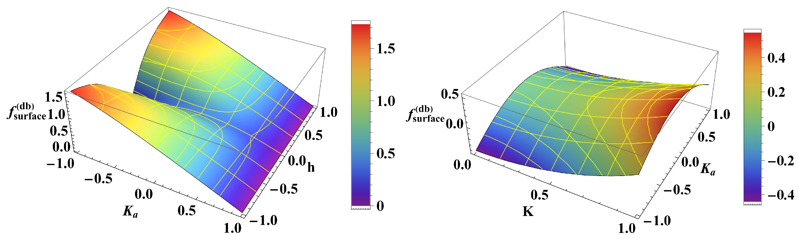
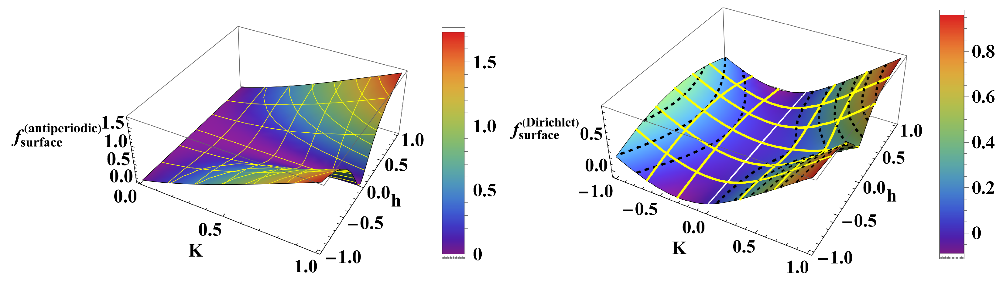
The behaviour of $f_{\mathrm{surface}}^{\left(\mathrm{antiperiodic}\right)}(K,h)$ and $f_{\mathrm{surface}}^{\left(\mathrm{free}\right)}(K,h)$ is visualised in Figure 1.

The surface free energy of the chain with a defect bond as a function of $K_a$, for specific choices of the parameters K and h, is shown in Figure 2.

7. Local Magnetisation in the Case of a Defect Bond

The average value ${\langle {\sigma }_n\rangle }_N^{\left(\tau \right)}$ of the random variable ${\sigma }_n$ under boundary conditions $\tau$ in a chain with N random variables is called in physical sciences site, or local, magnetisation. The dependence on the position n provides the so-called order parameter profile, which is of a special interest there.

In what follows, we compute the local magnetisation ${\langle {\sigma }_p\rangle }^{\left(db\right)}$ at lattice site p. By definition,

$${\langle {\sigma }_p\rangle }^{\left(db\right)}={\displaystyle \frac{1}{Z_{\mathrm{N}}^{\left(\mathrm{db}\right)}(K,K_a,h)}}\mathrm{Tr} \left({\mathbf{T}}_d {\mathbf{T}}^p {\mathit{\sigma }}_{\mathit{z}} {\mathbf{T}}^{N-1-p}\right).$$

(53)

The matrix ${\mathit{\sigma }}_{\mathit{z}}$ at a position p after the defect bond, is the Pauli matrix ${\mathit{\sigma }}_{\mathit{z}}=\mathrm{diag}(1,-1)$.

In what follows, we omit the superscript $\left(\tau \right)$ and replace it by $\left(db\right)$, with the understanding that we work throughout with the model subject to periodic boundary conditions with a defect bond; this convention introduces no ambiguity. Models with initial alternative boundary conditions are not considered in the present study.

We next introduces two auxiliary operator constructions,

$${\mathbf{D}}^p:={\mathbf{T}}_d {\tilde{\mathbf{T}}}^p, {\mathbf{L}}^{N-p-1}:={\mathit{\sigma }}_{\mathit{z}} {\tilde{\mathbf{T}}}^{ N-p-1}.$$

(54)

Using Equation (54), the definition for local magnetisation can be rewritten as

$${\langle {\sigma }_p\rangle }^{\left(db\right)}={\displaystyle \frac{{\left(\sqrt{2\sinh \left(2K\right)}\right)}^{N-1}}{Z_{\mathrm{N}}^{\left(\mathrm{db}\right)}(K,K_a,h)}}\mathrm{Tr}\left({\mathbf{D}}^{ p} {\mathbf{L}}^{ N-p-1}\right).$$

(55)

An immediate consequence of Lemma 1, which applies to matrix powers appearing under the trace, is that

$${\mathbf{D}}^{ p}=U_{p-1}\left(a\right) \left({\mathbf{T}}_d\tilde{\mathbf{T}}\right)-U_{p-2}\left(a\right) \left({\mathbf{T}}_d\mathbf{I}\right),$$

(56)

and

$${\mathbf{L}}^{N-p-1}=U_{N-p-2}\left(a\right) \left({\mathit{\sigma }}_{\mathit{z}}\tilde{\mathbf{T}}\right)-U_{N-p-3}\left(a\right) \left({\mathit{\sigma }}_{\mathit{z}}\mathbf{I}\right).$$

(57)

Consequently, the trace appearing on the right-hand side of Equation (55) becomes

$$\begin{array}{ccc}\hfill \mathrm{Tr} \left({\mathbf{D}}^p {\mathbf{L}}^{N-p-1}\right)& =& \mathrm{Tr} (\left\{U_{p-1}\left(a\right) \left({\mathbf{T}}_d\tilde{\mathbf{T}}\right)-U_{p-2}\left(a\right) \left({\mathbf{T}}_d\mathbf{I}\right)\right\}\hfill \\ & & \hfill \times \left\{U_{N-p-2}\left(a\right) \left({\mathit{\sigma }}_{\mathit{z}}\tilde{\mathbf{T}}\right)-U_{N-p-3}\left(a\right) \left({\mathit{\sigma }}_{\mathit{z}}\mathbf{I}\right)\right\}).\hfill \end{array}$$

(58)

Expanding the product and using linearity of the trace, the expression decomposes into four contributions:

$$\begin{array}{ccc}\hfill \mathrm{Tr} \left({\mathbf{D}}^p {\mathbf{L}}^{N-p-1}\right)& =& U_{p-1}\left(a\right) U_{N-p-2}\left(a\right) \mathrm{Tr} \left({\mathbf{T}}_d\tilde{\mathbf{T}}{\mathit{\sigma }}_{\mathit{z}}\tilde{\mathbf{T}}\right)\hfill \\ & & -U_{p-2}\left(a\right) U_{N-p-2}\left(a\right) \mathrm{Tr} \left({\mathbf{T}}_d\mathbf{I}{\mathit{\sigma }}_{\mathit{z}}\tilde{\mathbf{T}}\right)\hfill \\ & & -U_{p-1}\left(a\right) U_{N-p-3}\left(a\right) \mathrm{Tr} \left({\mathbf{T}}_d\tilde{\mathbf{T}}{\mathit{\sigma }}_{\mathit{z}}\mathbf{I}\right)\hfill \\ & & +U_{p-2}\left(a\right) U_{N-p-3}\left(a\right) \mathrm{Tr} \left({\mathbf{T}}_d\mathbf{I}{\mathit{\sigma }}_{\mathit{z}}\mathbf{I}\right).\hfill \end{array}$$

(59)

The trace terms appearing as four separate contributions in Equation (59) can be evaluated explicitly by direct matrix multiplication. These straightforward though somewhat tedious calculations yield the following results:

• the first term in Equation (59)

  $$\mathrm{Tr} \left({\mathbf{T}}_d\tilde{\mathbf{T}} {\mathit{\sigma }}_{\mathit{z}}\tilde{\mathbf{T}}\right)=2 {\mathrm{e}}^{K_a}\sinh \left(h\right)\left[4a^2-\coth \left(2K\right)-{\mathrm{e}}^{-2K_a} \mathrm{csch}\left(2K\right)\right];$$

  (60)
• the second term in Equation (59)

  $$\mathrm{Tr} \left({\mathbf{T}}_d {\mathit{\sigma }}_{\mathit{z}}\tilde{\mathbf{T}}\right)={\displaystyle \frac{2}{r}} {\mathrm{e}}^{K+K_a}\sinh \left(2h\right)=4a {\mathrm{e}}^{K_a}\sinh \left(h\right);$$

  (61)
• the third term in Equation (59)

  $$\mathrm{Tr} \left({\mathbf{T}}_d\tilde{\mathbf{T}} {\mathit{\sigma }}_{\mathit{z}}\right)={\displaystyle \frac{2}{r}} {\mathrm{e}}^{K+K_a}\sinh \left(2h\right)=4a {\mathrm{e}}^{K_a}\sinh \left(h\right);$$

  (62)
• the forth term in Equation (59)

  $$\mathrm{Tr} \left({\mathbf{T}}_d {\mathit{\sigma }}_{\mathit{z}}\right)=2 {\mathrm{e}}^{K_a}\sinh \left(h\right).$$

  (63)

We note that the observed coincidence of the second and third terms arises from cyclic permutation under the trace and the commutativity between the both transfer matrices ${\mathbf{T}}_d$ and $\tilde{\mathbf{T}}$. Upon substituting these results into Equation (59), and employing the recurrence relation (A2) for the Chebyshev polynomials of the second kind, we obtain

$$\begin{array}{c}Tr\left({\mathbf{D}}^p{\mathbf{L}}^{N-p-1}\right)=2e^{K_a}\sinh \left(h\right)\{F(K,K_a)U_{p-1}\left(a\right)U_{N-p-2}\left(a\right) \hfill \\ - 2a{U}_{p-1}\left(a\right)U_{N-p-3}\left(a\right)-U_{p-2}\left(a\right)U_{N-p-1}\left(a\right),\}\hfill \end{array}$$

(64)

where

$$F(K,K_a)=4a^2-(\coth \left(2K\right)-e^{-2K_a} \mathrm{csch}\left(2K\right)).$$

To complete our further consideration we need the following statement:

Proposition 2.

$$Tr\left({\mathbf{D}}^p {\tilde{\mathbf{L}}}^{N-p-1}\right)=U_p\left(a\right) U_{N-p-1}\left(a\right)-(\coth \left(2K\right)-e^{-2K_a} \mathrm{csch}\left(2K\right)) U_{p-1}\left(a\right) U_{N-p-2}\left(a\right).$$

(65)

Proof. 

Factoring out $4a^2$ from the first term and grouping it with the second and third terms in Equation (64), we obtain the following:

$$\begin{array}{c}4a^2{U}_{p-1}\left(a\right)U_{N-p-2}\left(a\right)-2a U_{p-1}\left(a\right)U_{N-p-3}\left(a\right)-U_{p-2}\left(a\right)U_{N-p-1}\left(a\right)\hfill \\ =2a{U}_{p-1}\left(a\right)[2a{U}_{N-p-2}\left(a\right)-U_{N-p-3}\left(a\right)]-U_{p-2}\left(a\right)U_{N-p-1}\left(a\right).\hfill \end{array}$$

(66)

Using the standard recurrence relation for Chebyshev polynomials of the second kind (see, Equation (A3)),

$$U_{n+1}\left(a\right)=2a{U}_n\left(a\right)-U_{n-1}\left(a\right),$$

(67)

with $n=N-p-2$, this expression simplifies to

$$[2a{U}_{p-1}\left(a\right)-U_{p-2}\left(a\right)]U_{N-p-1}\left(a\right).$$

(68)

Applying again, but with $n=p-1$, Equation (67) to the term in brackets in the second line of Equation (66), we arrive to the conclusion that it reduces to the single product $U_p\left(a\right)U_{N-p-1}\left(a\right)$. Finally, substituting this back into the trace expression and keeping the remaining $F(K,K_a)$ term, we obtain

$$\mathrm{Tr}\left({\mathbf{D}}^p{\mathbf{L}}^{N-p-1}\right)=U_p\left(a\right) U_{N-p-1}\left(a\right)-(\coth \left(2K\right)-e^{-2K_a} \mathrm{csch}\left(2K\right)) U_{p-1}\left(a\right) U_{N-p-2}\left(a\right),$$

which proves the proposition. □

Using the result of Proposition 2, together with Equation (55), we arrive at

Theorem 3.

Let ${\langle {\sigma }_p\rangle }^{\left(db\right)}$ denote the local magnetisation at site p of a periodic spin chain containing a single defect bond with arbitrary coupling $K_a$. Then

$$\begin{array}{cc}& {\langle {\sigma }_p\rangle }^{\left(db\right)}={\displaystyle \frac{e^{K_a} \sinh \left(h\right)}{2(a^2-1)}}\hfill \\ \times & {\displaystyle \frac{{\displaystyle T_{N+1}\left(a\right)-T_{2p-N+1}\left(a\right)-\left(\coth \left(2K\right)-e^{-2K_a} \mathrm{csch}\left(2K\right)\right)\left(T_{N-1}\left(a\right)-T_{2p-N+1}\left(a\right)\right)}}{{\displaystyle e^{K_a}\cosh \left(h\right) U_{N-1}\left(a\right)-\frac{2\sinh (K+K_a)}{r\left(K\right)} U_{N-2}\left(a\right)}}}.\hfill \end{array}$$

(69)

Proof. 

Starting from Equation (55) and using Proposition 2, as well as the identities

$$\begin{array}{cc}\hfill U_p\left(a\right)U_{N-p-1}\left(a\right) & ={\displaystyle \frac{T_{N+1}\left(a\right)-T_{2p-N+1}\left(a\right)}{2(a^2-1)}},\hfill \end{array}$$

(70)

$$\begin{array}{cc}\hfill U_{p-1}\left(a\right)U_{N-p-2}\left(a\right) & ={\displaystyle \frac{T_{N-1}\left(a\right)-T_{2p-N+1}\left(a\right)}{2(a^2-1)}},\hfill \end{array}$$

(71)

for the numerator in Equation (69) we obtain

$$T_{N+1}\left(a\right)-T_{2p-N+1|}\left(a\right)-\left(\coth \left(2K\right)-e^{-2K_a} \mathrm{csch(2K)}\right)\left(T_{N-1}\left(a\right)-T_{2p-N+1}\left(a\right)\right).$$

Realising that the denominator arises from the partition function in Equation (23), we immediately arrive at Equation (69). □

8. Limiting Cases of $\mathbf{:}{\mathit{K}}_{\mathit{a}}=\mathit{K},{\mathit{K}}_{\mathit{a}}=\mathbf{0},{\mathit{K}}_{\mathit{a}}=-\mathit{K}$

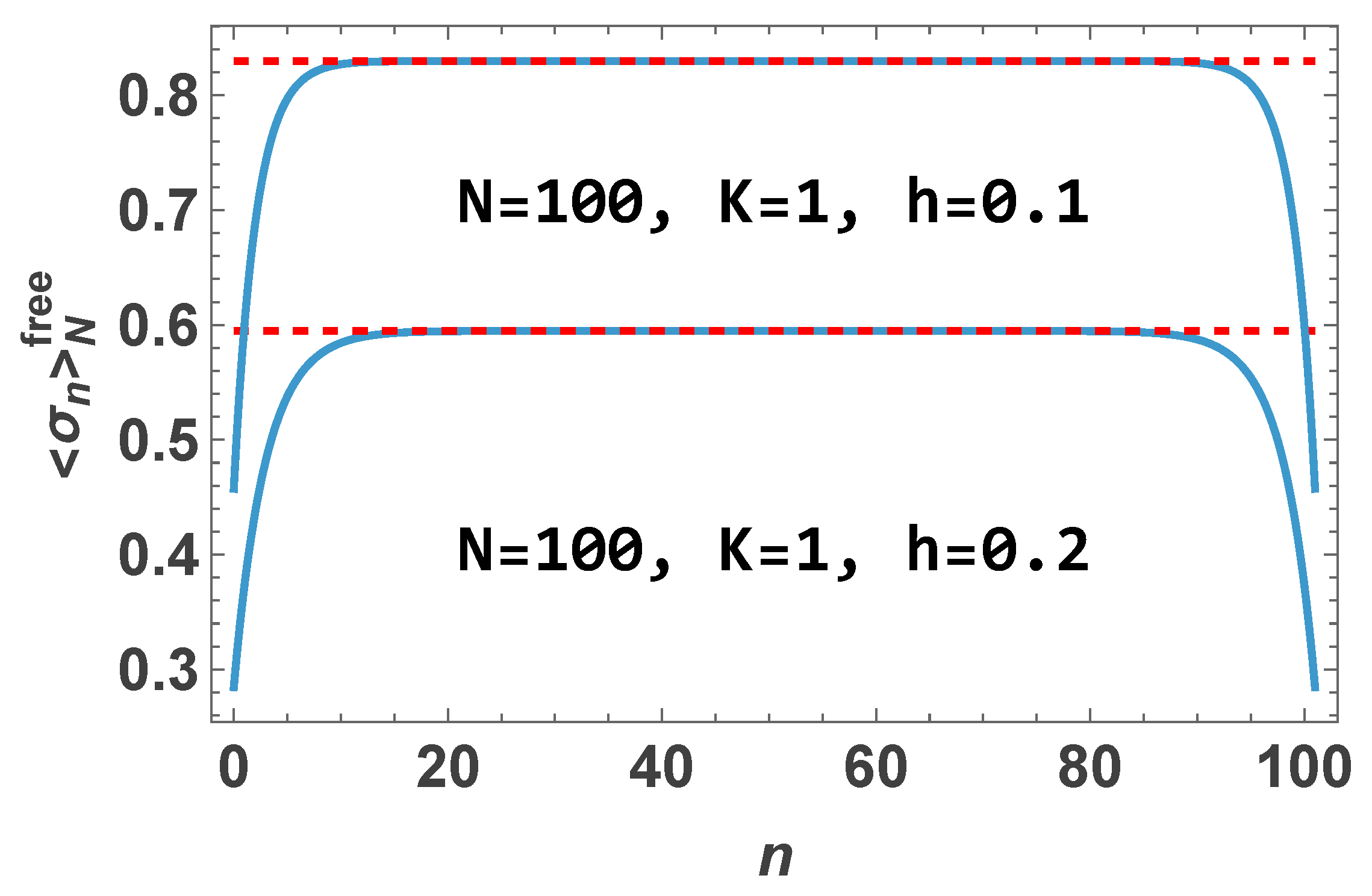
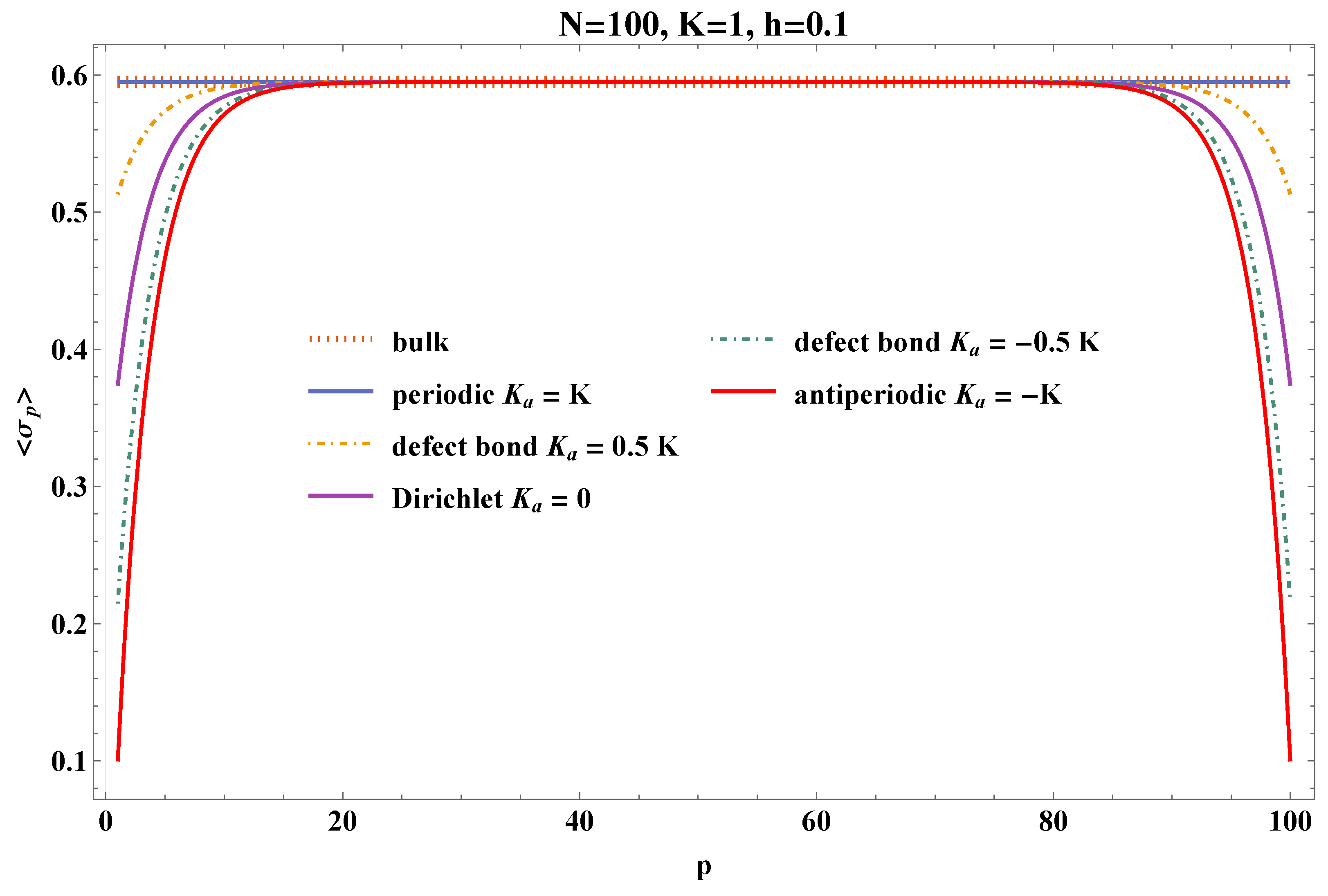
The behaviour of the order parameter profile under different boundary conditions is shown in Figure 3.

Below we derive analytical expressions for the order parameter profiles for the special cases with $K_a=-K$ free (Dirichlet), $K_a=K$ (periodic), and $K_a=-K$ (antiperiodic) boundary conditions, of interest in physical sciences.

Corollary 3.

Consequently, we obtain the following:

• free (Dirichlet) boundary conditions:
  Setting $K_a=0$ in Theorem 3, we get

  $${\langle {\sigma }_p\rangle }^{\left(\mathrm{free}\right)}={\displaystyle \frac{\sinh \left(h\right)}{2(a^2-1)}}{\displaystyle \frac{{\displaystyle T_{N+1}\left(a\right)-T_{2p-N+1}\left(a\right)-\tanh \left(K\right) \left(T_{N-1}\left(a\right)-T_{2p-N+1}\left(a\right)\right)}}{{\displaystyle \cosh \left(h\right) U_{N-1}\left(a\right)-\sqrt{\tanh \left(K\right)} U_{N-2}\left(a\right),}}}.$$

  (72)

  where, for $K_a=0$, the grand-canonical partition function reduces to

  $$Z_N^{\left(\mathrm{db}\right)}(K,0,h)=2r^{N-1}\left[\cosh \left(h\right) U_{N-1}\left(a\right)-\sqrt{\tanh \left(K\right)} U_{N-2}\left(a\right)\right].$$

  (73)
  Another representation of the ${\langle {\sigma }_p\rangle }^{\left(\mathrm{free}\right)}$, but in terms of the Chebyshev $U_n\left(z\right)$ polynomial, instead of $T_n\left(z\right)$, is

  $${\langle {\sigma }_n\rangle }_N^{\left(\mathrm{free}\right)}=\sinh \left(h\right){\displaystyle \frac{\left[U_{n-1}\left(a\right)U_{N-n}\left(a\right)-\tanh \left(K\right)U_{n-2}\left(a\right)U_{N-n-1}\left(a\right)\right]}{\left\{\cosh \left(h\right) U_{N-1}\left(a\right)-\sqrt{\tanh \left(K\right)} U_{N-2}\left(a\right)\right\}}}.$$

  (74)
  Comparing Equation (74) with Equation (65), one establishes the equivalence of both results.

Remark 6.

The explicit dependence on p remains because the system is not translation invariant. Different positions p correspond to different relative locations of the insertion “defect bond matrix” in the product ${\tilde{\mathcal{D}}}^p{\tilde{\mathcal{L}}}^{N-p-1}$. This manifests mathematically in the appearance of the modes $T_{N-2p-1}\left(a\right)$ and $T_{N-2p+1}\left(a\right)$ in the trace formula.

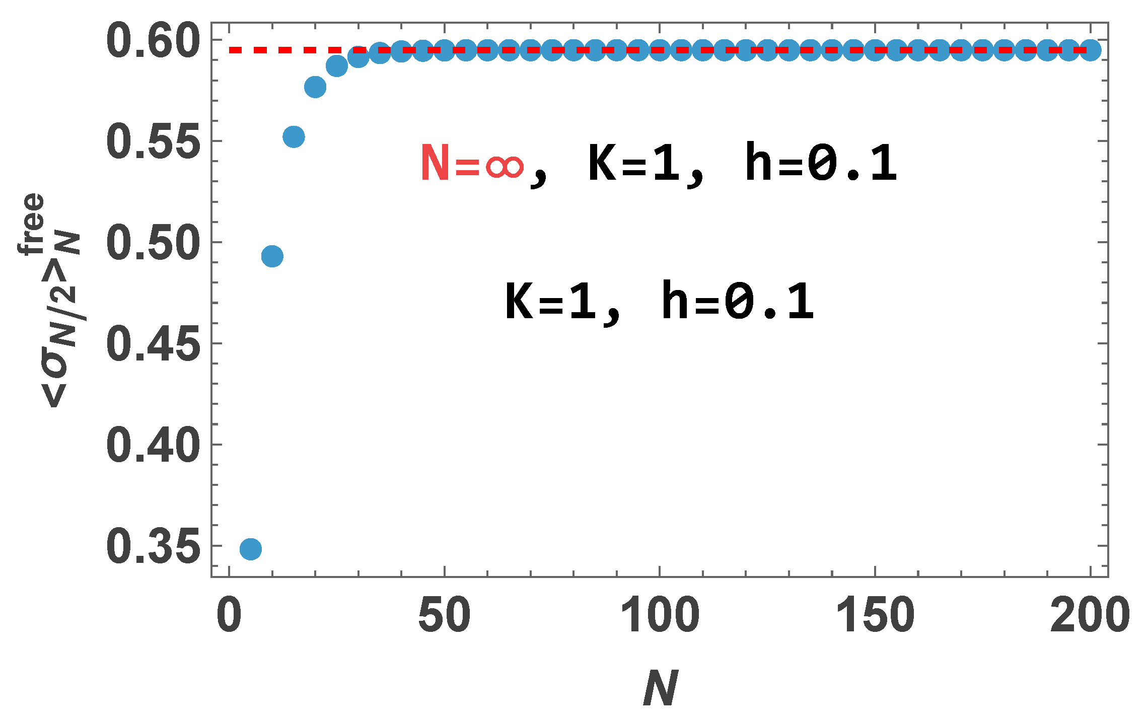
The behaviour of the order parameter profile given by Equation (74) is depicted in Figure 4.

Figure 5 shows how fast, with the increase of N, the average value of the random variable positioned in the middle of the chain approaches the corresponding limit of the infinite (bulk) system.

• Periodic Boundary Conditions:
  In this case $K_a=K$. Setting in Equation (55) $K_a=K$, and using the w partition function $Z_N^{\left(\mathrm{periodic}\right)}(K,h)$ in this case, is given by the following equation:

  $$Z_N^{\left(\mathrm{periodic}\right)}(K,h)=2{\left[\sqrt{2\sinh \left(2K\right)}\right]}^N{T}_N\left(a\right).$$

  (75)

  we derive

  $${\langle {\sigma }_p\rangle }^{\left(\mathrm{periodic}\right)}=\tanh \left(h\right) a {\displaystyle \frac{U_N\left(a\right)}{T_N\left(a\right)}}.$$

  (76)
  This result was recently obtained in [31]. It demonstrates that the site magnetisation is independent of p, which is consistent with the expectation for periodic boundary conditions.
• Antiperiodic Boundary Conditions
  In this case $K_a=-K$, i.e., all bonds have the same coupling constant K, except for one with $K_a=-K$. Then, the local magnetisation at site p is given by the following equation:

  $${\langle {\sigma }_p\rangle }^{\left(\mathrm{antiperiodic}\right)}={\displaystyle \frac{{\left(\sqrt{2\sinh \left(2K\right)}\right)}^{N-1}}{Z_N^{\left(\mathrm{antiperiodic}\right)}(K,h)}}\mathrm{Tr}\left({\tilde{\mathcal{D}}}^p{\tilde{\mathcal{L}}}^{N-p-1}\right).$$

  (77)
  In this case

  $$\begin{array}{ccc}\hfill Tr\left({\tilde{\mathcal{D}}}^p {\tilde{\mathcal{L}}}^{N-p-1}\right)& =& 2e^{-K}\sinh \left(h\right)\left\{U_p\left(a\right) U_{N-p-1}\left(a\right)+ U_{p-1}\left(a\right) U_{N-p-2}\left(a\right)\right\}\hfill \\ & =& 2e^{-K}\sinh \left(h\right){\displaystyle \frac{T_{N-2p-1}\left(a\right)-a T_N\left(a\right)}{1-a^2}},\hfill \end{array}$$

  (78)

  where we have used the recurrence relation

  $$U_p\left(a\right)U_{N-p-1}\left(a\right)+U_{p-1}\left(a\right)U_{N-p-2}\left(a\right)={\displaystyle \frac{T_{N-1}\left(a\right)-T_{2p-N}\left(a\right)}{1-a^2}}.$$

  (79)
  The partition function is given by

  $$Z_N^{\left(\mathrm{antiperiodic}\right)}(K,h)=2e^{-2K}{r}^N a U_{N-1}\left(a\right).$$

  (80)
  Then

  $${\langle {\sigma }_p\rangle }^{\left(\mathrm{antiperiodic}\right)}={\displaystyle \frac{\tanh \left(h\right)[T_{N-2p+1}\left(a\right)-a{T}_N\left(a\right)]}{(1-a^2)U_{N-1}\left(a\right)}}.$$

  (81)
  This result was recently obtained in [31].

Remark 7.

The explicit dependence on p reflects the absence of translation invariance in the system. Indeed, the trace $Tr\left({\tilde{\mathcal{D}}}^p{\tilde{\mathcal{L}}}^{ N-p-1}\right)$ contains a multiplication by the “defect matrix” ${\mathbf{T}}_d$ at a position p, so different values of p are not related by symmetry. Mathematically, this manifests itself in the appearance of the mode $T_{N-2p-1}\left(a\right)$, which encodes the relative distance of the insertion of the defect bond from the boundaries. Only in a translation-invariant limit, as in periodic boundary conditions, does the p-dependence disappear.

Remark 8.

In conclusion, we note that by varying the parameter $K_a$, we can model a continuum of boundary conditions imposed on the chain, which include as special cases the most important ones: periodic ($K_a=K$), antiperiodic ($K_a=-K$), and free (Dirichlet) ($K_a=0$) boundary conditions.

9. Conclusions

We have proposed a new method for calculating quantities in the one-dimensional Ising model based on the properties of the Chebyshev polynomials. We have shown that the recurrence structure of the Chebyshev polynomials of the second kind $U_n\left(x\right)$ is naturally embedded in the transfer-matrix formulation of the model, especially suitable for studies of the cases with broken translational invariance. One example, which we employed, is caused by a defective bond at a specific site. The mathematical framework of our approach relies on two key elements: the algebra of $2\times 2$ matrices and the systematic exploitation of various recurrence relations among Chebyshev polynomials. This formulation provides a unified and technically convenient method.

Using the method suggested in this article, we obtain explicit expressions for the expectations $\mathbb{E}\left[{\sigma }_p\right]$ of the random variables ${\sigma }_p$, see Equation (53), in a one-dimensional Ising chain, highlighting their dependence on the site index p relative to the defect bond $K_a$; this defines the profile of the local magnetisation. In physical sciences this profile is also called the order parameter profile. The analytical result is given in Equation (69). The visualisation of the expression for different values of $K_a$ is presented in Figure 3. Note that by varying the value of $K_a$, one recovers periodic boundary conditions for $K_a=K$, antiperiodic boundary conditions for $K_a=-K$, and Dirichlet (free) boundary conditions for $K_a=0$. We stress that the result for the last case is also new, and to the best of our knowledge, has never been derived before. Equation (72) provides an expression for the profile linear in terms of Chebyshev $T_n\left(z\right)$ polynomials, while Equation (74) provides an equivalent expression in terms of products of $U_n\left(z\right)$ polynomials. Figure 4 demonstrates the behaviour of the profile for free boundary conditions when $N=100$, and two set of values of the parameters governing the system. Finally, Figure 5 illustrates how fast, with the increase of N, the behaviour of the system approaches the corresponding one of the infinite chain.

The normalisation factor in the denominator of Equation (1) is called the partition function in statistical physics. Through it, one defines the free energy of the system (see Equations (23) and (46)), which is of primary interest in physical sciences. In Section 5 we briefly discuss the behaviour of this quantity for periodic, antiperiodic, and Dirichlet (free) boundary conditions, as well as for the case of a system with a defect bond. As shown there, for a large number N of random variables, i.e., when $N\gg 1$, the free energy can be decomposed into a part which does not depend on N, characterising the system with an infinite number of random variables, plus one $\mathcal{O}(1/N)$ term, called surface free energy, see Equation (47). The behaviour of the surface free energy as a function of the parameters of the model is shown in Figure 1 and Figure 2.

We close this short discussion by stressing that the method proposed here is by no means limited to studying of the quantities considered in the current article. It can be straightforwardly extended, e.g., to investigate other quantities of interest in physical sciences, say, the correlation functions, the role of impurities, or the existence of some structures inside of the finite system.

References

- McCoy, B.M.; Wu, T.T. The Two-Dimensional Ising Model; Harvard University Press: Cambridge, MA, USA, 1973. [Google Scholar]
- Baxter, R.J. Exactly Solved Models in Statistical Mechanics; Academic Press: London, UK, 1982. [Google Scholar]
- Marchi, E.; Vila, J. Recursive Method in One-Dimensional Ising Model. J. Phys. A Math. Gen. 1980, 13, 2465. [Google Scholar] [CrossRef]
- Kassan-ogly, F.A. One-dimensional Ising model with next-nearest-neighbour interaction in magnetic field. Phase Transit. A Multinatl. J. 2001, 74, 353–365. [Google Scholar] [CrossRef]
- Antal, T.; Droz, M.; Rácz, Z. Probability distribution of magnetization in the one-dimensional Ising model: Effects of boundary conditions. J. Phys. A Math. Gen. 2004, 37, 1465. [Google Scholar]
- Bellucci, S.; Ohanyan, V. Correlation functions in one-dimensional spin lattices with Ising and Heisenberg bonds. Eur. Phys. J. B 2013, 86, 446. [Google Scholar] [CrossRef][Green Version]
- Seth, S. Combinatorial Approach to Exactly Solve the 1D Ising Model. Eur. J. Phys. 2016, 38, 015104. [Google Scholar] [CrossRef]
- da Conceição, C.S.; Maia, R. Recurrence relations in one-dimensional Ising models. Phys. Rev. E 2017, 96, 032121. [Google Scholar] [CrossRef]
- Kharchenko, Y.N. On the Solution of One-Dimensional Ising Models. J. Appl. Math. Phys. 2018, 6, 84525. [Google Scholar] [CrossRef][Green Version]
- Magare, S.; Roy, A.; Srivastava, V. 1D Ising model using the Kronecker sum and Kronecker product. Eur. J. Phys. 2022, 43, 035102. [Google Scholar] [CrossRef]
- Ferreira, L.S.; Plascak, J.A. Finite-Size Effects of the One-Dimensional Ising Model. Braz. J. Phys. 2023, 53, 77. [Google Scholar] [CrossRef]
- Wortis, M. Griffiths singularities in the randomly dilute one-dimensional Ising model. Phys. Rev. B 1974, 10, 4665. [Google Scholar] [CrossRef]
- Shigematsu, H. Asymptotic behavior of fluctuations for the 1D Ising model in zero-temperature limit. J. Stat. Phys. 1993, 71, 981–1002. [Google Scholar] [CrossRef]
- García-Pelayo, R. Distribution of magnetization in the finite Ising chain. J. Math. Phys. 2009, 50, 013301. [Google Scholar] [CrossRef]
- Rudnick, J.; Zandi, R.; Shackell, A.; Abraham, D. Boundary conditions and the critical Casimir force on an Ising model film: Exact results in one and two dimensions. Phys. Rev. E 2010, 82, 041118. [Google Scholar] [CrossRef] [PubMed][Green Version]
- Taherkhani, F.; Daryaei, E.; Parsafar, G.; Fortunelli, A. Investigation of size effects on the physical properties of one-dimensional Ising models in nanosystems. Mol. Phys. 2011, 109, 385–395. [Google Scholar] [CrossRef]
- Chiruta, D.; Linares, J.; Miyashita, S.; Boukheddaden, K. Role of open boundary conditions on the hysteretic behaviour of one-dimensional spin crossover nanoparticles. J. Appl. Phys. 2014, 115, 194309. [Google Scholar] [CrossRef]
- Balcerzak, T. Application of the integral operator method for multispin correlation function calculations in the one-dimensional Ising model. Phys. Rev. E 2024, 109, 024133. [Google Scholar] [CrossRef]
- Balog, I.; Rançon, A. Constraint correlation functions of the one-dimensional Ising model in the scaling limit. Phys. Rev. E 2025, 112, 054127. [Google Scholar] [CrossRef]
- Abelès, F. Recherches sur la propagation des ondes électromagnétiques sinusoïdales dans les milieux stratifiés. Applications aux couches minces (Research on the propagation of sinusoidal electromagnetic waves in stratified media. Applications to thin films). Ann. Phys. 1950, 12, 596–640, 706–782. [Google Scholar] [CrossRef]
- Jones, H. The electron energy spectrum in long period superlattices. J. Phys. F Met. Phys. 1973, 3, 2075–2085. [Google Scholar]
- Sprung, D.W.L.; Wu, H.; Martorell, J. Scattering by a finite periodic potential. Am. J. Phys. 1993, 61, 1118–1123. [Google Scholar] [CrossRef]
- Wu, H.; Sprung, D.W.L.; Martorell, J. Periodic Quantum Wires and Their Quasi-One Dimensional Nature. J. Phys. D Appl. Phys. 1993, 26, 798–803. [Google Scholar] [CrossRef]
- Griffiths, D.J.; Steinke, C.A. Waves in locally periodic media. Am. J. Phys. 2001, 69, 137–154. [Google Scholar] [CrossRef]
- Furman, S.A.; Tikhonravov, A.V. Basics of Optics of Multilayer Systems; Atlantica Séguier Frontieres: Paris, France, 1992. [Google Scholar]
- Born, M.; Wolf, E. Section 1.6: Wave propagation in a stratified medium. Theory of dielectric films. In Principles of Optics: Electromagnetic Theory of Propagation, Interference and Diffraction of Light, 7th ed.; Cambridge University Press: Cambridge, UK, 1999; Chapter 1.6; pp. 54–65. [Google Scholar]
- Sánchez-Soto, L.L.; Monzón, J.J.; Barriuso, A.G.; Cariñena, J.F. The transfer matrix: A geometrical perspective. Phys. Rep. 2012, 513, 191–227. [Google Scholar] [CrossRef]
- Pereyra, P. The transfer matrix method and the theory of finite periodic systems. From heterostructures to superlattices. Phys. Status Solidi (b) 2022, 259, 2100405. [Google Scholar] [CrossRef]
- Dantchev, D.M.; Tonchev, N.S.; Rudnick, J. Casimir versus Helmholtz forces: Exact results. Ann. Phys. 2023, 459, 169533. [Google Scholar] [CrossRef]
- Dantchev, D.M.; Tonchev, N.; Rudnick, J. Casimir and Helmholtz forces in one-dimensional Ising model with Dirichlet (free) boundary conditions. Ann. Phys. 2024, 464, 169647. [Google Scholar] [CrossRef]
- Tonchev, N.S.; Dantchev, D. Chebyshev Polynomials in the Physics of the One-Dimensional Finite-Size Ising Model: An Alternative View and Some New Results. Condens. Matter 2024, 9, 53. [Google Scholar] [CrossRef]
- Brandi, R.; Ricci, P.E. Composition Identities of Chebyshev Polynomials via 2 × 2 Matrix Powers. Symmetry 2020, 12, 746. [Google Scholar] [CrossRef]
- Doman, B.; Williams, J. Low-temperature properties of frustrated Ising chains. J. Phys. C Solid State Phys. 1982, 15, 1693. [Google Scholar] [CrossRef]
- Rehn, J.; Santos, F.; Coutinho-Filho, M. Combinatorial and topological analysis of the Ising chain in a field. Braz. J. Phys. 2012, 42, 410–421. [Google Scholar] [CrossRef]
- Snyder, M. Chebyshev Methods in Numerical Approximation; Prentice Hall, Inc.: Englewood Cliffs, NJ, USA, 1966. [Google Scholar]
- Koshy, T. Fibonacci and Lucas Numbers with Applications, Volume 2; John Wiley & Sons: Hoboken, NJ, USA, 2019; Volume 2. [Google Scholar]
- Smajlović, L.; Šabanac, Z.; Šćeta, L. Relations between Chebyshev, Fibonacci and Lucas polynomials via trigonometric sums. Fibonacci Q. 2025, 63, 439–455. [Google Scholar] [CrossRef]
- Dantchev, D.; Tonchev, N. A Brief Survey of Fluctuation-Induced Interactions in Micro and Nano-Systems and One Exactly Solvable Model as Example. In Advanced Computing in Industrial Mathematics. BGSIAM 2023; Lilkova, E., Datcheva, M., Aleksandrova, T., Eds.; Studies in Computational Intelligence; Springer: Cham, Switzerland, 2025; Volume 1219, pp. 44–58. [Google Scholar] [CrossRef]
- Mason, J.C.; Handscomb, D.C. Chebyshev Polynomials; CRC Press: Boca Raton, FL, USA, 2002. [Google Scholar]
- Binder, K. Critical Behaviour at Surfaces. In Phase Transitions and Critical Phenomena; Domb, C., Lebowitz, J.L., Eds.; Academic Press: London, UK, 1983; Volume 8, Chapter 1; pp. 1–145. [Google Scholar]
- Privman, V. Finite-size scaling theory. In Finite Size Scaling and Numerical Simulations of Statistical Systems; Privman, V., Ed.; World Scientific: Singapore, 1990; pp. 1–98. [Google Scholar]
- Privman, V. (Ed.) Finite Size Scaling and Numerical Simulation of Statistical Systems; World Scientific: Singapore, 1990; p. 1. [Google Scholar]
- Brankov, J.G.; Dantchev, D.M.; Tonchev, N.S. The Theory of Critical Phenomena in Finite-Size Systems—Scaling and Quantum Effects; World Scientific: Singapore, 2000. [Google Scholar]
- Dantchev, D.M.; Dietrich, S. Critical Casimir effect: Exact results. Phys. Rep. 2023, 1005, 1–130. [Google Scholar] [CrossRef]