High-Order Difference Scheme for Time-Fractional Quasilinear Parabolic Equations

Abstract

Mathematical modeling of heat and mass transfer processes in porous media using fractional derivative equations is of great practical importance. Within the framework of such models, obtaining analytical solutions to the corresponding initial–boundary value problems is generally difficult. In this work, we numerically investigate quasilinear parabolic problems involving Caputo time-fractional derivatives. First, the well-posedness and existence of weak solutions are discussed. Then, we construct and implement a finite-difference scheme that is fourth-order accurate in space and second-order accurate in time. Convergence in the maximum norm is proven. Numerical experiments confirm the accuracy and efficiency of the proposed approach.

1. Introduction

Time-fractional parabolic problems typically model phenomena that exhibit memory effects or hereditary behavior, such as heat conduction in porous media, diffusion in heterogeneous materials, or viscoelastic deformation [1,2,3,4,5,6]. In such models, the classical first-order time derivative is replaced by a fractional one, most often of Caputo type, to account for the nonlocal dependence of the present state on its entire past history. These problems are characterized by weakly singular solutions and nonlocal temporal operators, which make their analytical treatment difficult and motivate the development of accurate and efficient numerical methods [7,8].

Time-fractional linear diffusion problems have been studied by many authors; see, for example, [9,10,11,12,13,14].

When the diffusion coefficient depends on the solution itself, the problem becomes nonlinear (quasilinear), describing processes where the diffusivity varies with temperature, concentration, or pressure. Such nonlinear time-fractional parabolic equations arise, for instance, in nonlinear heat conduction, infiltration in porous media, and anomalous transport in heterogeneous materials, and their numerical analysis presents additional challenges due to both the fractional and nonlinear nature of the governing operator; see, e.g., [15,16,17].

In [18,19], analytical properties of the time-fractional porous medium equation with nonlinear diffusion depending on a power of the solution were investigated, including the existence, uniqueness, and qualitative behavior of compactly supported solutions. The existence, uniqueness, regularity, comparison principle, and decay rates for the doubly nonlocal porous medium equation were established in [2]. The existence and uniqueness and a second-order finite difference scheme for the time-fractional Barenblatt-type problem were constructed in [20,21,22]. For the same problem, the authors of [15] analyzed self-similar solutions using an integral equation approach that extends classical results to the fractional setting.

The study [16] further considered the time-fractional quasilinear porous medium equation. The model was reformulated using Erdélyi–Kober fractional integrals, and numerical simulations were performed to illustrate the qualitative behavior of compactly supported solutions. In [23], global strong solvability of the time-fractional quasilinear initial-boundary value problem was established. More recently, in [24], classical solutions to time-fractional quasilinear reaction–diffusion systems were constructed and analyzed, providing additional insight into the regularity and qualitative behavior of related fractional parabolic models. Numerical aspects of solving quasilinear time-fractional diffusion equations were addressed in [25], where a regularized mesh scheme was proposed for the efficient and stable approximation of such problems. Further contributions include the work [17], which studied anomalous non-self-similar infiltration in porous media described by a fractional diffusion equation with a variable-order time derivative and nonlinear diffusivity, demonstrating good empirical convergence of the proposed schemes. In addition, the structure-preserving scheme developed in [26] for fractional quasilinear diffusion equations was shown to be first-order accurate in time and to exhibit superlinear spatial convergence in the fractional porous-medium regime, while preserving key qualitative properties such as algebraic decay and finite-time extinction.

Different numerical methods have been developed for time-fractional semilinear parabolic equations, where the right-hand side depends on the solution and the time derivative is of fractional order $\alpha \in (0,1)$. High-order schemes have been constructed for this class of problems, rather than for general time-fractional nonlinear parabolic equations. In [27], a rigorous numerical framework was proposed for such problems, establishing stability and optimal error estimates for both spatial and temporal discretizations, with second-order accuracy in space and $\alpha$-order accuracy in time. In [28], to handle the weak singularity of the solution, a $(3-\alpha )$-order $L2-1_{\sigma }$ scheme on nonuniform meshes was employed for the temporal discretization, while the finite element method was applied for the spatial approximation. The method proposed in [29] combines a cubic time-stepping approximation with a compact finite difference scheme in space, achieving convergence of order $(4-\alpha )$ in time and fourth-order accuracy in space for sufficiently smooth solutions. In [30], the authors developed a high-order computational technique for semilinear time-fractional reaction–diffusion problems exhibiting an initial singularity. Their approach uses a graded-mesh $L2-1_{\sigma }$ time discretization together with a parametric quintic spline in space, effectively reducing the impact of the singularity and attaining temporal accuracy of order $min\{r\alpha ,2\}$ and spatial accuracy of about $4.5$ in the $L_2$ norm, where r controls the mesh grading. In general, high-order numerical schemes have mainly been developed for such semilinear problems, while corresponding results for fully nonlinear time-fractional parabolic equations remain scarce.

In contrast to semilinear formulations, where the nonlinearity appears only in lower-order terms, the quasilinear structure considered here requires a different treatment of the diffusion operator.

Despite numerous analytical and numerical studies on time-fractional nonlinear parabolic problems, to the best of our knowledge, numerical schemes with fourth-order spatial accuracy for time-fractional quasilinear parabolic problems have not yet been developed and analyzed.

In this work, we consider a Caputo time-fractional quasilinear parabolic problem. The aim of the present paper is to construct and analyze a high-order numerical approximation.

We establish the well-posedness of the differential problem. A compact fourth-order spatial discretization is developed and combined with the $L2-1_{\sigma }$ time-stepping scheme on a graded mesh to address the weak singularity of the solution. Conceptually, the proposed approach extends the compact discretization idea used for linear and semilinear problems; however, the presence of solution-dependent diffusion requires a different treatment in both the scheme construction and error analysis. Newton’s iterative method is employed to handle the resulting nonlinear discrete system.

In the present paper, we consider the one-dimensional time-fractional quasilinear diffusion equation [16,23]

$${\displaystyle \frac{{\partial }^{\alpha }p}{\partial t^{\alpha }}}={\displaystyle \frac{\partial }{\partial x}}\left(k\left(p\right){\displaystyle \frac{\partial p}{\partial x}}\right)+f(x,t),(x,t)\in Q_T=\Omega \times (0,T),\Omega =(c,d),$$

(1)

where $k\left(p\right)\ge k_0>0$; ${\displaystyle \frac{{\partial }^{\alpha }}{\partial t^{\alpha }}}$ is the the Caputo fractional derivative of order $\alpha$, $0<\alpha <1$, defined by

$${\displaystyle \frac{{\partial }^{\alpha }p(x,t)}{\partial t^{\alpha }}=\frac{1}{\Gamma (1-\alpha )}{\int }_0^t\frac{\partial p(x,s)}{\partial s}{(t-s)}^{-\alpha };}$$

and $\Gamma (·)$ denotes the Gamma function.

The Equation (1) is subjected to initial and boundary conditions:

$$\begin{array}{ccc}& & p(x,0)=p_0\left(x\right),x\in (c,d),\hfill \end{array}$$

(2)

$$\begin{array}{ccc}& & p(c,t)=p_l\left(t\right),p(d,t)=p_r\left(t\right),t\in [0,T].\hfill \end{array}$$

(3)

In the next section, we first introduce some basic definitions and a formula from fractional calculus and then establish the well-posedness of the direct problem.

The remaining part of this paper is organized as follows. In Section 2, the well-posedness of the model problem is discussed. Section 3 is devoted to the description of a high-order finite difference scheme that is second-order accurate in time and fourth-order accurate in space. In Section 4, the convergence in the maximum norm is investigated. Results from numerical test examples are presented and discussed in Section 5. This paper is finalized with some concluding remarks.

2. Well-Posedness of the Differential Problems

In this section, we investigate the existence and uniqueness of solutions to problems (1)–(3).

2.1. Fractional Integrals and Derivatives

First, we recall the basic definitions of fractional differentiation and integration of the Riemann–Liouville and Caputo types [6,31,32,33]. Namely, if $g\left(t\right)\in L(0,T)$, then for $\alpha >0$, the Riemann–Liouville (R-L) left-sided integral $J_{0^{+}}^{\alpha }g$ and right-sided integral $J_{T^{-}}^{\alpha }g$ are defined by

$$J_{0^{+}}^{\alpha }g\left(t\right)={\displaystyle \frac{1}{\Gamma \left(\alpha \right)}}\underset{0}{\overset{t}{\int }}{\displaystyle \frac{g\left(s\right)ds}{{(t-s)}^{1-\alpha }}},0<t\le T$$

and

$$J_{T^{-}}^{\alpha }g\left(t\right)={\displaystyle \frac{1}{\Gamma \left(\alpha \right)}}\underset{t}{\overset{T}{\int }}{\displaystyle \frac{g\left(s\right)ds}{{(s-t)}^{1-\alpha }}},0\le t<T.$$

If $g\left(t\right)\in AC[0,T]$, then for $0<\alpha <1$, the R-L left-sided fractional derivative $D_{0^{+}}^{\alpha }g$ and right-sided fractional derivative $D_{T^{-}}^{\alpha }g$ of order $\alpha$ are defined by

$$D_{0^{+}}^{\alpha }g\left(t\right)={\displaystyle \frac{1}{\Gamma (1-\alpha )}}{\displaystyle \frac{d}{dt}}\underset{0}{\overset{t}{\int }}{\displaystyle \frac{g\left(s\right)ds}{{(t-s)}^{\alpha }}}:={\displaystyle \frac{d}{dt}}\left(J_{0^{+}}^{1-\alpha }g\right)\left(t\right),0<t\le T$$

and

$$D_{T^{-}}^{\alpha }g\left(t\right)=-{\displaystyle \frac{1}{\Gamma (1-\alpha )}}{\displaystyle \frac{d}{dt}}\underset{t}{\overset{T}{\int }}{\displaystyle \frac{g\left(s\right)ds}{{(s-t)}^{\alpha }}}:=-{\displaystyle \frac{d}{dt}}\left(J_{T^{-}}^{1-\alpha }g\right)\left(t\right),0\le t<T.$$

Next, if $g\left(t\right)\in AC[0,T]$, then for $0<\alpha <1$, the Caputo left-sided fractional derivative ${}^{C}D_{0^{+}}^{\alpha }g$ and right-sided fractional derivative ${}^{C}D_{T^{-}}^{\alpha }g$ of order $\alpha$ are defined by

$${}^{C}D_{0^{+}}^{\alpha }g\left(t\right)={\displaystyle \frac{{\partial }^{\alpha }g\left(t\right)}{\partial t^{\alpha }}},0<t\le T$$

and

$${}^{C}D_{T^{-}}^{\alpha }g\left(t\right)=-{\displaystyle \frac{1}{\Gamma (1-\alpha )}}\underset{t}{\overset{T}{\int }}{\displaystyle \frac{g^{\prime }\left(s\right)ds}{{(s-t)}^{\alpha }}}:=-\left(J_{T^{-}}^{1-\alpha }{g}^{\prime }\right)\left(t\right),0\le t<T.$$

Further, we use the following integration by parts formula. Let $w\left(t\right)\in AC[0,T]$, $w^{\prime }\left(t\right)\in C_{1-\alpha }[0,T]$, $v\left(t\right)\in C[0,T]$, $D_{T^{-}}^{\alpha }v\in L(0,T)$, and $0<\alpha <1$; then,

$$\underset{0}{\overset{T}{\int }}{\displaystyle \frac{{\partial }^{\alpha }w\left(t\right)}{\partial t^{\alpha }}}v\left(t\right)dt=w\left(T\right)\left(J_{T^{-}}^{1-\alpha }v\right)\left(T\right)-w\left(0\right)\left(J_{T^{-}}^{1-\alpha }v\right)\left(0\right)+\underset{0}{\overset{T}{\int }}w\left(t\right)\left(D_{T^{-}}^{\alpha }v\right)\left(t\right)dt.$$

(4)

2.2. Existence and Uniqueness of the Solution

In this subsection, we discuss the existence and uniqueness of the solution to problems (1)–(3), following some results of [34]. Namely, the authors introduce on $I:=[0,\infty )$ the class of admissible coefficients $k\left(p\right)$ as follows:

$$k\left(p\right)\in C\left(I\right),k_0\le k\left(p\right)\le k_1\mathrm{for}\mathrm{all}p\in I,$$

(5)

and satisfy the monotonicity condition

$${\int }_{\Omega }\left(k\left(p_1\right){\displaystyle \frac{\partial p_1}{\partial x}}-k\left(p_2\right){\displaystyle \frac{\partial p_2}{\partial x}}\right){\displaystyle \frac{\partial }{\partial x}}(p_1-p_2)dx\ge k_2{∥{\displaystyle \frac{\partial }{\partial x}}(p_1-p_2)∥}_{L^2(\Omega )}^2$$

(6)

for all $p_1,p_2\in H^1(\Omega )$, where $k_0$, $k_1$, and $k_2$ are positive constants.

Let v be an arbitrary test function such that $v\in L^2(0,T;H^1(\Omega ))$, $D_{T^{-}}^{\alpha }v\in L^2(0,T;L^2(\Omega ))$, and $v(·,T)=0$.

Multiplying Equation (1) by v and integrating over $Q_T$, and using the fractional integration by parts Formula (4), we obtain the weak formulation (7):

$$\begin{array}{cc}\hfill & -{\int }_0^T{\int }_{\Omega }p(x,t)D_{T^{-}}^{\alpha }v(x,t)dxdt+{\int }_0^T{\int }_{\Omega }k\left(p\right){\displaystyle \frac{\partial p}{\partial x}}{\displaystyle \frac{\partial v}{\partial x}}dxdt\hfill \\ \hfill & ={\int }_0^T{\int }_{\Omega }f(x,t)v(x,t)dxdt+{\int }_{\Omega }{p}_0\left(x\right)\left(J_{T^{-}}^{1-\alpha }v\right)(0,x)dx.\hfill \end{array}$$

(7)

Due to the nonhomogeneous Dirichlet boundary conditions (3), a standard boundary shifting technique is applied to reduce the problem to an equivalent problem with homogeneous boundary conditions. Under assumptions (5)–(6) on the coefficient $k\left(p\right)$, Theorem 3.1 in [34] guarantees the existence and uniqueness of a weak solution to the reduced problem.

Consequently, problems (1)–(3) admit a unique weak solution $p\in L^2(0,T;H^1(\Omega ))\cap W_2^{\alpha }(0,T;L^2(\Omega )),$ in the sense of (7). Moreover, the weak solution satisfies the a priori estimate

$${\int }_0^T{\parallel p(·,t)\parallel }_{H^1(\Omega )}^{2}dt\le C\left({\parallel f\parallel }_{L^2\left(Q_T\right)}^2+{\parallel p_0\parallel }_{L^2(\Omega )}^2\right),$$

where $C>0$ is a constant independent of p.

Further, for the construction and analysis of numerical solutions, we assume that the exact solution p possesses the following regularity, which is typical of time-fractional diffusion problems with weak initial singularities [7,8]:

$$\begin{array}{ccc}& & \left|{\displaystyle \frac{{\partial }^{j}p}{\partial t^j}}(x,t)\right|\le C_1\left(1+t^{\alpha -j}\right),0\le j\le 3,\hfill \\ & & \left|{\displaystyle \frac{{\partial }^{j}p}{\partial x^j}}(x,t)\right|\le C_2,0\le j\le 4,\hfill \end{array}$$

for all $(x,t)\in [c,d]\times (0,T]$ and positive constants $C_1$ and $C_2$, and $p(·,t)\in C^4\left(\overline{\Omega }\right)$ uniformly for $t\in [0,T]$.

3. Numerical Method

We consider a uniform spatial mesh and a nonuniform temporal mesh in the rectangle $Q_T$: ${\overline{w}}_{h\tau }={\overline{w}}_h\times {\overline{w}}_{\tau }$, where

$${\overline{w}}_h=\left\{x_i=c+ih,i=0,1,\dots ,I,h=(d-c)/I\right\},w_h={\overline{w}}_h\setminus \{x_0,x_I\},$$

$${\overline{w}}_{\tau }=\left\{t_n=t_{n-1}+{\tau }_n,n=1,\dots ,N,t_0=0,t_N=T\right\}.$$

Further, we denote $p_i=p_i\left(t\right)=p(x_i,t)$, $x_i\in {\overline{w}}_h$, and $P_i^n$ is the approximation of p at grid node $(x_i,t_n)\in {\overline{w}}_{h\tau }$.

We consider the problems (1), (2), and (3) and rewrite Equation (1) in the form

$${\displaystyle \frac{{\partial }^{\alpha }p}{\partial t^{\alpha }}}={\displaystyle \frac{{\partial }^2}{\partial x^2}}\left(K\left(p\right)\right)+f(x,t),$$

(8)

where

$${\displaystyle \frac{d}{dp}}\left(K\left(p\right)\right)={\left(K\left(p\right)\right)}^{\prime }=k\left(p\right).$$

Using the well-known approximation (p. 74, [35])

$$u_{\overline{x}x,i}={\displaystyle \frac{u\left(x_{i-1}\right)-2u\left(x_i\right)+u\left(x_{i+1}\right)}{h^2}}={\displaystyle \frac{d^{2}u}{d{x}^2}}\left(x_i\right)+{\displaystyle \frac{h^2}{12}}{\displaystyle \frac{d^{4}u}{d{x}^4}}\left(x_i\right)+O\left(h^4\right),x_i\in w_h,$$

we derive

$${\left(K\left(p\right)\right)}_{\overline{x}x,i}={\displaystyle \frac{{\partial }^2}{\partial x^2}}{\left.\left(K\right(p\left)\right)\right|}_{x=x_i}+{\displaystyle \frac{h^2}{12}}{\displaystyle \frac{{\partial }^4}{\partial x^4}}{\left.\left(K\right(p\left)\right)\right|}_{x=x_i}+O\left(h^4\right),$$

(9)

From (8) and (9), we obtain

$$\begin{array}{c}\hfill \begin{array}{cc}\hfill {\displaystyle \frac{{\partial }^{\alpha }{p}_i}{\partial t^{\alpha }}}=& {\left(K\left(p\right)\right)}_{\overline{x}x,i}-{\displaystyle \frac{h^2}{12}}{\displaystyle \frac{{\partial }^4}{\partial x^4}}{\left.\left(K\right(p\left)\right)\right|}_{x=x_i}+f(t,x_i),x_i\in w_h.\hfill \end{array}\end{array}$$

(10)

Next, differentiating Equation (8) twice with respect to x and evaluating the result at the point $x_i\in w_h$ yields

$${\left.{\displaystyle \frac{{\partial }^2}{\partial x^2}}{\displaystyle \frac{{\partial }^{\alpha }p}{\partial t^{\alpha }}}\right|}_{x=x_i}={\left.{\displaystyle \frac{{\partial }^4}{\partial x^2}}\left(K\left(p\right)\right)\right|}_{x=x_i}+{\left.{\displaystyle \frac{{\partial }^{2}f}{\partial x^2}}\right|}_{x=x_i}.$$

(11)

Then, from (10) and (11), we derive $O\left(h^4\right)$ spatial semidiscretization of (8):

$${\displaystyle \frac{{\partial }^{\alpha }{p}_i}{\partial t^{\alpha }}}+{\left.{\displaystyle \frac{h^2}{12}}{\displaystyle \frac{{\partial }^2}{\partial x^2}}{\displaystyle \frac{{\partial }^{\alpha }p}{\partial t^{\alpha }}}\right|}_{x=x_i}={\left(K\left(p\right)\right)}_{\overline{x}x,i}+{\displaystyle \frac{h^2}{12}}{\left.{\displaystyle \frac{{\partial }^{2}f}{\partial x^2}}\right|}_{x=x_i}+f(x_i,t),x_i\in w_h,$$

which can be written as

$${\left.{\displaystyle \frac{{\partial }^{\alpha }}{\partial t^{\alpha }}}\left(p+{\displaystyle \frac{h^2}{12}}{\displaystyle \frac{{\partial }^{2}p}{\partial x^2}}\right)\right|}_{x=x_i}={\left(K\left(p\right)\right)}_{\overline{x}x,i}+{\displaystyle \frac{h^2}{12}}{\left.{\displaystyle \frac{{\partial }^{2}f}{\partial x^2}}\right|}_{x=x_i}+f(x_i,t)x_i\in w_h.$$

(12)

For the temporal derivative, we consider the $L2-1_{\sigma }$ formula obtained in [36], for a uniform temporal mesh with step size $\tau$. It is of order $O\left({\tau }^{3-\alpha }\right)$ at $(x_i,t_{n+\sigma })$, $t_{n+\sigma }=(n+\sigma )\tau$, $\sigma =1-\alpha /2$, $n=0,1,\dots ,N-1$ for solutions $u\left(t\right)\in C^3[0,T]$.

In this work, we apply the $L2-1_{\sigma }$ formula on a nonuniform temporal mesh [7,8]. Let $t_{n+\sigma }=t_n+\sigma {\tau }_{n+1}$. Thus, the fractional temporal derivative is approximated as follows:

$${\displaystyle \frac{{\partial }^{\alpha }p}{\partial t^{\alpha }}}{|}_{(x_i,t_{n+\sigma })}\approx D_{t_{n+\sigma }}^{\alpha }{P}_i:=g_{n,n}{P}_i^{n+1}-\sum _{j=0}^n\left(g_{n,j}-g_{n,j-1}\right)P_i^j,n=0,1,\dots ,N-1.$$

(13)

Here, we set $g_{n,-1}:=0$, ${\displaystyle g_{0,0}=\frac{1}{{\tau }_1}{a}_{0,0}}$, and for $n\ge 1$,

$$g_{n,j}=\left\{\begin{array}{cc}{\displaystyle \frac{1}{{\tau }_{j+1}}(a_{n,0}-b_{n,0}),}\hfill & j=0,n\ge 1,\hfill \\ {\displaystyle \frac{1}{{\tau }_{j+1}}(a_{n,j}+b_{n,j}-b_{n,j-1}),}\hfill & 1\le j\le n-1,\hfill \\ {\displaystyle \frac{1}{{\tau }_{n+1}}(a_{n,n}+b_{n,n-1}),}\hfill & j=n,\hfill \end{array}\right.$$

where

$$\begin{array}{ccc}\hfill a_{n,n}& =& {\displaystyle \frac{1}{\Gamma (1-\alpha )}}{\int }_{t_n}^{t_{n+\sigma }}{(t_{n+\sigma }-s)}^{-\alpha }ds={\displaystyle \frac{{\sigma }^{1-\alpha }}{\Gamma (2-\alpha )}}{\tau }_{n+1}^{1-\alpha },n\ge 0,\hfill \\ \hfill a_{n,j}& =& {\displaystyle \frac{1}{\Gamma (1-\alpha )}}{\int }_{t_j}^{t_{j+1}}{(t_{n+\sigma }-s)}^{-\alpha }ds,n\ge 1,0\le j\le n-1,\hfill \\ \hfill b_{n,j}& =& {\displaystyle \frac{1}{2\Gamma (1-\alpha )(t_{j+2}-t_j)}}{\int }_{t_j}^{t_{j+1}}{(t_{n+\sigma }-s)}^{-\alpha }\left(s-\frac{t_j+t_{j+1}}{2}\right)ds,n\ge 1.\hfill \end{array}$$

Here, $D_{t_{n+\sigma }}^{\alpha }{P}_i$ denotes the L2-1_σ approximation of the Caputo fractional derivative ${\displaystyle \frac{{\partial }^{\alpha }p}{\partial t^{\alpha }}}(x_i,t_{n+\sigma })$, that is, the temporal discretization is performed at the fixed spatial node $x=x_i$ and at time $t_{n+\sigma }$.

Using (12) and (13), we construct the $\sigma$- weighted finite difference approximation of (8):

$$\begin{array}{c}\hfill \begin{array}{cc}\hfill D_{t_{n+\sigma }}^{\alpha }\left(P_i+{\displaystyle \frac{h^2}{12}}{P}_{\overline{x}x,i}\right)& =\sigma {\left(K\left(P^{n+1}\right)\right)}_{\overline{x}x,i}+(1-\sigma ){\left(K\left(P^n\right)\right)}_{\overline{x}x,i}\hfill \\ & +{\displaystyle \frac{h^2}{12}}{\displaystyle \frac{{\partial }^{2}f}{\partial x^2}}(x_i,t_{n+\sigma })+f(x_i,t_{n+\sigma }),i=1,2,\dots ,I-1.\hfill \end{array}\end{array}$$

(14)

Therefore, the discretization of the problems (1) and (2) is (3) and (14) with initial and boundary conditions:

$$\begin{array}{c}\hfill \begin{array}{cc}\hfill & P_i^0=p_0\left(x_i\right),i=0,1,\dots ,I,\hfill \\ & P_0^{n+1}=p_l\left(t_{n+1}\right),P_I^{n+1}=p_r\left(t_{n+1}\right).\hfill \end{array}\end{array}$$

(15)

4. Convergence

In this section, we establish the convergence of the numerical scheme (14) and (15) in the maximum norm. We consider the following nonuniform temporal mesh [7,8,28,37]:

$$t_n=T{\left({\displaystyle \frac{n}{N}}\right)}^r,r\ge 1,n=0,1,\dots ,N.$$

(16)

The weak singularity of the solution near $t=0$ limit the convergence order on uniform time meshes. Graded temporal mesh (16) concentrates time steps near the initial time to better resolve this behavior. The grading parameter r determines the strength of this refinement and must be chosen appropriately to recover the optimal convergence rate [7,8].

First, we derive the local truncation error.

Lemma 1.

Let $p(·,t)\in C^4\left(\overline{\Omega }\right)$ uniformly for $t\in [0,T]$. Moreover, for each fixed $x\in \overline{\Omega }$, $p(x,·)\in C[0,T]\cap C^3(0,T]$ and ${\displaystyle \frac{{\partial }^{2}p}{\partial x^2}}p(x,·)\in C[0,T]\cap C^3(0,T]$. Suppose that the exact solution of (1)–(3) is bounded, i.e., there exists a constant $C_p>0$ such that $0\le p(x,t)\le C_p\mathrm{for}\mathrm{all}(x,t)\in {\overline{Q}}_T,$ and let $D_p=[0,C_p]$. Assume that $K\in C^2\left(D_p\right)$. Then, the local truncation error $\mathcal{T}(x_i,t_{n+\sigma })$ at the grid point $(x_i,t_{n+\sigma })$, $n=0,1,\dots ,N-1$, satisfies

$$\mathcal{T}(x_i,t_{n+\sigma })=O\left(N^{-min\{2,r\alpha \}}\right)+O\left(h^4\right),i=1,2,\dots ,I-1.$$

(17)

Proof. 

Applying the results in [8] (see Lemma 1 and Lemma 7), for each fixed $x\in \Omega$, we get

$$\begin{array}{c}\hfill \begin{array}{cc}\hfill & \left|D_{t_{n+\sigma }}^{\alpha }\left(p\left(x,·\right)\right)-{\displaystyle \frac{{\partial }^{\alpha }}{\partial t^{\alpha }}}p(x,t_{n+\sigma })\right|\le C_3{t}_{n+\sigma }^{-\alpha }{N}^{-min\{3-\alpha ,r\alpha \}},0\le \sigma \le 1,\hfill \\ & {\displaystyle \left|D_{t_{n+\sigma }}^{\alpha }\left(\frac{{\partial }^{2}p}{\partial x^2}\left(x,·\right)\right)-\frac{{\partial }^{\alpha }}{\partial t^{\alpha }}\frac{{\partial }^{2}p}{\partial x^2}(x,t_{n+\sigma })\right|\le C_4{t}_{n+\sigma }^{-\alpha }{N}^{-min\{3-\alpha ,r\alpha \}},0\le \sigma \le 1,}\hfill \end{array}\end{array}$$

(18)

Further, using Lemma 9 [8], for each fixed $x\in \Omega$, we obtain

$${\displaystyle \left|\sigma p(x,t_{n+1})+(1-\sigma )p(x,t_n)-p(x,t_{n+\sigma })\right|\le \frac{{\tau }_{n+1}^2}{8}\underset{t_n<t<t_{n+1}}{max}\left|\frac{{\partial }^{2}p}{\partial t^2}(x,t)\right|=:C_5{\tau }_{n+1}^2.}$$

Taking into account that $K\in C^2\left(D_p\right)$, we apply the same argument as in the proof of Lemma 9 in [8] to deduce that for each fixed $x\in \Omega$,

$$\begin{array}{c}\hfill \begin{array}{cc}\hfill & \left|\sigma K\left(p(x,t_{n+1})\right)+(1-\sigma )K\left(p(x,t_n)\right)-K\left(p(x,t_{n+\sigma })\right)\right|\hfill \\ & \le {\displaystyle \frac{{\tau }_{n+1}^2}{8}}\underset{t_n<t<t_{n+1}}{max}\left|K^{″}(p(x,t)){\left({\displaystyle \frac{\partial }{\partial t}}p(x,t)\right)}^2+K^{\prime }(p(x,t)){\displaystyle \frac{{\partial }^2}{\partial t^2}}p(x,t)\right|=:C_6{\tau }_{n+1}^2.\hfill \end{array}\end{array}$$

(19)

Indeed, for fixed $x\in \Omega$ and $1\le n\le N-1$, Taylor’s series expansion yields

$$\begin{array}{ccc}\hfill K(p(x,t_{n+1}))& =& K\left(p(x,t_{n+\sigma })\right)+K^{\prime }(p(x,t_{n+\sigma })){\displaystyle \frac{\partial }{\partial t}}p(x,t_{n+\sigma })(1-\sigma ){\tau }_{n+1}\hfill \\ & & +{\displaystyle \frac{1}{2}}\left[K^{″}(p(x,{\xi }_1)){\left({\displaystyle \frac{\partial }{\partial t}}p(x,{\xi }_1)\right)}^2+K^{\prime }(p(x,{\xi }_1)){\displaystyle \frac{{\partial }^2}{\partial t^2}}p(x,{\xi }_1)\right]{(1-\sigma )}^2{\tau }_{n+1}^2,\hfill \\ \hfill K(p(x,t_n))& =& K(p(x,t_{n+\sigma }))-K^{\prime }\left(p(x,t_{n+\sigma })\right){\displaystyle \frac{\partial }{\partial t}}p(x,t_{n+\sigma })\sigma {\tau }_{n+1}\hfill \\ & & +{\displaystyle \frac{1}{2}}\left[K^{″}(p(x,{\xi }_2)){\left({\displaystyle \frac{\partial }{\partial t}}p(x,{\xi }_2)\right)}^2+K^{\prime }(p(x,{\xi }_2)){\displaystyle \frac{{\partial }^2}{\partial t^2}}p(x,{\xi }_2)\right]{\sigma }^2{\tau }_{n+1}^2,\hfill \end{array}$$

where ${\xi }_1,{\xi }_2\in (t_n,t_{n+1})$.

Therefore, for each fixed $x\in \Omega$, we obtain

$$\begin{array}{ccc}& & \left|\sigma K\left(p(x,t_{n+1})\right)+(1-\sigma )K\left(p(x,t_n)\right)-K\left(p(x,t_{n+\sigma })\right)\right|\hfill \\ & =& {\displaystyle \frac{1}{2}}\left|\left(K^{″}(p(x,{\xi }_1)){\left({\displaystyle \frac{\partial }{\partial t}}p(x,{\xi }_1)\right)}^2+K^{\prime }(p(x,{\xi }_1)){\displaystyle \frac{{\partial }^2}{\partial t^2}}p(x,{\xi }_1)\right)\sigma {(1-\sigma )}^2{\tau }_{n+1}^2\right.\hfill \\ & & \left.+\left(K^{″}(p(x,{\xi }_2)){\left({\displaystyle \frac{\partial }{\partial t}}p(x,{\xi }_2)\right)}^2+K^{\prime }(p(x,{\xi }_2)){\displaystyle \frac{{\partial }^2}{\partial t^2}}p(x,{\xi }_2)\right)(1-\sigma ){\sigma }^2{\tau }_{n+1}^2\right|,\hfill \end{array}$$

which implies (19).

Further, in view of (18), the local truncation error of (14) is

$$\begin{array}{ccc}\hfill \mathcal{T}(x_i,t_{n+\sigma })& =& D_{t_{n+\sigma }}^{\alpha }\left(p(x_i,·)+{\displaystyle \frac{h^2}{12}}{p}_{\overline{x}x}(x_i,·)\right)-\sigma {\left(K\left(p(x_i,t_{n+1})\right)\right)}_{\overline{x}x,i}\hfill \\ & & -(1-\sigma ){\left(K\left(p(x_i,t_n)\right)\right)}_{\overline{x}x,i}-{\displaystyle \frac{h^2}{12}}{\displaystyle \frac{{\partial }^{2}f}{\partial x^2}}(x_i,t_{n+\sigma })-f(x_i,t_{n+\sigma })\hfill \\ & =& {\displaystyle \frac{{\partial }^{\alpha }}{\partial t^{\alpha }}}\left(p(x_i,t_{n+\sigma })+{\displaystyle \frac{h^2}{12}}{\left[p(x_i,t_{n+\sigma })\right]}_{\overline{x}x,i}\right)+O\left(N^{-min\{3-\alpha ,r\alpha \}}\right)\hfill \\ & & -{\left[K\left(p(x_i,t_{n+\sigma })\right)\right]}_{\overline{x}x,i}+O\left({\tau }_{n+1}^2\right)-{\displaystyle \frac{h^2}{12}}{\displaystyle \frac{{\partial }^{2}f}{\partial x^2}}(x_i,t_{n+\sigma })-f(x_i,t_{n+\sigma }).\hfill \end{array}$$

From (9), we derive

$$\begin{array}{ccc}\hfill \mathcal{T}(x_i,t_{n+\sigma })& =& {\displaystyle \frac{{\partial }^{\alpha }}{\partial t^{\alpha }}}\left(p(x_i,t_{n+\sigma })+{\displaystyle \frac{h^2}{12}}{\displaystyle \frac{{\partial }^{2}p}{\partial x^2}}(x_i,t_{n+\sigma })\right)+O\left(N^{-min\{3-\alpha ,r\alpha \}}\right)\hfill \\ & & -{\displaystyle \frac{{\partial }^2}{\partial x^2}}\left(K\left(p(x_i,t_{n+\sigma })\right)\right)-{\displaystyle \frac{h^2}{12}}{\displaystyle \frac{{\partial }^4}{\partial x^4}}\left(K\left(p(x_i,t_{n+\sigma })\right)\right)+O\left(h^4\right)\hfill \\ & & +O\left({\tau }_{n+1}^2\right)-{\displaystyle \frac{h^2}{12}}{\displaystyle \frac{{\partial }^{2}f}{\partial x^2}}(x_i,t_{n+\sigma })-f(x_i,t_{n+\sigma }),i=1,2,\dots ,I-1.\hfill \end{array}$$

Finally, using (8) and (11), we obtain (17). □

Let

$$(u,v)=h\sum _{i=1}^{I-1}{u}_i{v}_i,{\parallel u\parallel }^2:=(u,u).$$

Theorem 1.

Under the conditions of Lemma 1 and assumptions (5) and (6), the numerical solution of (14)–(15) satisfies the following error estimate:

$$\underset{0\le n\le N}{max}\parallel P^n-p\left(t_n\right)\parallel \le C\left(N^{-min\{2,r\alpha \}}+h^4\right),$$

(20)

where $C>0$ is a constant independent of h and N.

Proof. 

Let $P^n:={(P_1^n,\dots ,P_{I-1}^n)}^T$ and $p^n:={(p(x_1,t_n),\dots ,p(x_{I-1},t_n))}^T$, and denote $e^n:=p^n-P^n$.

For any grid function $U^n={(U_1^n,\dots ,U_{I-1}^n)}^T$, we define the $\mathbf{A}$$\in {\mathbb{R}}^{(I-1)\times (I-1)}$ corresponding to the second-order difference operator with homogeneous Dirichlet boundary conditions ${\left(\mathbf{A}{U}^n\right)}_i=-U_{\overline{x}x,i}^n=-\left(U_{i+1}^n-2U_i^n+U_{i-1}^n\right)/h^2$, $1\le i\le I-1$, with the convention $U_0^n=U_I^n=0$. Note that $\mathbf{A}$ is symmetric positive definite. Moreover, although the original problem is subject to nonhomogeneous Dirichlet boundary conditions, the error $e^n$ satisfies homogeneous boundary conditions, which motivates the use of the operator $\mathbf{A}$.

Next, we define the compact averaging matrix

$$\mathbf{B}:=\mathbf{I}-{\displaystyle \frac{h^2}{12}}\mathbf{A},$$

so that ${\left(\mathbf{B}{U}^n\right)}_i=U_i^n+{\displaystyle \frac{h^2}{12}}{U}_{\overline{x}x,i}^n$ for $1\le i\le I-1$. The matrix $\mathbf{B}$ is symmetric positive definite and invertible.

For vectors $U^n$, we set $K\left(U^n\right):={(K\left(U_1^n\right),\dots ,K\left(U_{I-1}^n\right))}^T$. We also define the $\sigma$–weighted average

$$U^{n+\sigma }:=\sigma U^{n+1}+(1-\sigma )U^n,e^{n+\sigma }:=\sigma e^{n+1}+(1-\sigma )e^n,$$

(21)

which will be used in the diffusion term of scheme (14).

Further, we write (14) in vector form. Using the notation

$$D_{t_{n+\sigma }}^{\alpha }\left(\mathbf{B}P\right):={\left(D_{t_{n+\sigma }}^{\alpha }\left(\mathbf{B}{P}_1\right),\dots ,D_{t_{n+\sigma }}^{\alpha }\left(\mathbf{B}{P}_{I-1}\right)\right)}^T,$$

scheme (14) becomes

$$D_{t_{n+\sigma }}^{\alpha }\left(\mathbf{B}P\right)=-\sigma \mathbf{A}K\left(P^{n+1}\right)-(1-\sigma )\mathbf{A}K\left(P^n\right)+F^{n+\sigma },n=0,1,\dots ,N-1,$$

(22)

where $F^{n+\sigma }\in {\mathbb{R}}^{I-1}$ collects the known source terms $\left(f+{\displaystyle \frac{h^2}{12}}{\displaystyle \frac{{\partial }^{2}f}{\partial x^2}}\right)(x_i,t_{n+\sigma })$, $i=1,\dots ,I-1$.

By definition of the local truncation error, substituting the exact solution componentwise into (22) yields

$$D_{t_{n+\sigma }}^{\alpha }\left(\mathbf{B}p\right)=-\sigma \mathbf{A}K\left(p^{n+1}\right)-(1-\sigma )\mathbf{A}K\left(p^n\right)+F^{n+\sigma }+{\mathcal{T}}^{n+\sigma }.$$

(23)

Here, ${\mathcal{T}}^{n+\sigma }$ denotes the vector of local truncation errors evaluated at the time level $t_{n+\sigma }$, i.e.,

$${\mathcal{T}}^{n+\sigma }:={\left(\mathcal{T}(x_1,t_{n+\sigma }),\dots ,\mathcal{T}(x_{I-1},t_{n+\sigma })\right)}^T.$$

Subtracting (23) from (22) gives the error equation

$$D_{t_{n+\sigma }}^{\alpha }\left(\mathbf{B}e\right)=-\sigma \mathbf{A}\left(K\left(P^{n+1}\right)-K\left(p^{n+1}\right)\right)-(1-\sigma )\mathbf{A}\left(K\left(P^n\right)-K\left(p^n\right)\right)-{\mathcal{T}}^{n+\sigma },$$

(24)

with $e^0=\mathbf{0}$, where all equalities and operators are understood componentwise and the homogeneous boundary conditions for $e^n$ are incorporated into the definition of $\mathbf{A}$.

Multiplying (24) by $h{e}_i^{n+\sigma }$ and summing over $i=1,\dots ,I-1$, we get

$$(D_{t_{n+\sigma }}^{\alpha }\left(\mathbf{B}e\right),e^{n+\sigma })+(\mathbf{A}{\Phi }^{n+\sigma },e^{n+\sigma })=({\mathcal{T}}^{n+\sigma },e^{n+\sigma }),$$

(25)

where ${\Phi }^{n+\sigma }=\sigma {\Phi }^{n+1}+(1-\sigma ){\Phi }^n$, ${\Phi }^m:=K\left(p^m\right)-K\left(P^m\right)$.

Denote $U_{x,i}^n:=(U_{i+1}^n-U_i^n)/h$, and recall the summation-by-parts identity

$$(-U_{\overline{x}x}^n,V^n)=(U_x^n,V_x^n):=h\sum _{i=0}^{I-1}{U}_{x,i}^n{V}_{x,i}^n\mathrm{for}{U}_0^n=U_I^n=0,V_0^n=V_I^n=0.$$

For the spatial term in (25), by summation-by-parts, we derive

$$(\mathbf{A}{\Phi }^{n+\sigma },e^{n+\sigma })=\left({\Phi }_x^{n+\sigma },e_x^{n+\sigma }\right).$$

(26)

Next, we use the discrete analogy of (6). Note that (6) can be written in the form

$${\int }_{\Omega }{\displaystyle \frac{\partial }{\partial x}}\left(K\left(p_1\right)-K\left(p_2\right)\right){\displaystyle \frac{\partial }{\partial x}}(p_1-p_2)dx\ge k_2{∥{\displaystyle \frac{\partial }{\partial x}}(p_1-p_2)∥}_{L^2(\Omega )}^2,$$

(27)

Now, let $V,U\in {\mathbb{R}}^{I-1}$ be arbitrary grid functions with $V_0=V_I=U_0=U_I=0$, and let $v_h,u_h\in H_0^1(\Omega )$ be their continuous piecewise-linear interpolants on the mesh ${\overline{w}}_h$, i.e., $v_h\left(x_i\right)=V_i$ and $u_h\left(x_i\right)=U_i$ for $i=0,1,\dots ,I$. Then, on each subinterval $(x_i,x_{i+1})$,

$${\displaystyle \frac{\partial v_h}{\partial x}}\left(x\right)=V_{x,i},{\displaystyle \frac{\partial u_h}{\partial x}}\left(x\right)=U_{x,i},x\in (x_i,x_{i+1}),$$

and, hence,

$${∥{\displaystyle \frac{\partial }{\partial x}}(v_h-u_h)∥}_{L^2(\Omega )}^2=\sum _{i=0}^{I-1}{\int }_{x_i}^{x_{i+1}}{(V-U)}_{x,i}^{2}dx=h\sum _{i=0}^{I-1}{(V-U)}_{x,i}^2=:{\parallel {(V-U)}_x\parallel }^2.$$

Applying (27) with $p_1=v_h$ and $p_2=u_h$ gives

$${\int }_{\Omega }{\displaystyle \frac{\partial }{\partial x}}\left(K\left(v_h\right)-K\left(u_h\right)\right){\displaystyle \frac{\partial }{\partial x}}(v_h-u_h)dx\ge k_2{∥{\displaystyle \frac{\partial }{\partial x}}(v_h-u_h)∥}_{L^2(\Omega )}^2.$$

(28)

Since ${\displaystyle \frac{\partial }{\partial x}}(v_h-u_h)$ is constant on each subinterval $(x_i,x_{i+1})$, we can evaluate the integral in (28) on each subinterval to obtain

$$h\sum _{i=0}^{I-1}\left({\left(K\left(V\right)\right)}_{x,i}-{\left(K\left(U\right)\right)}_{x,i}\right){(V-U)}_{x,i}\ge k_2{\parallel {(V-U)}_x\parallel }^2,$$

namely,

$$\left({(K\left(V\right)-K\left(U\right))}_x,{(V-U)}_x\right)\ge k_2{\parallel {(V-U)}_x\parallel }^2.$$

In particular, taking $V=p^{n+\sigma }$ and $U=P^{n+\sigma }$ componentwise, so that ${\Phi }^{n+\sigma }=K\left(V\right)-K\left(U\right)$ and $e^{n+\sigma }=V-U$, and using (26), we derive

$$(\mathbf{A}{\Phi }^{n+\sigma },e^{n+\sigma })\ge k_2{\parallel e_x^{n+\sigma }\parallel }^2.$$

(29)

Further, we define ${\parallel u\parallel }_{\mathbf{B}}^2:=(\mathbf{B}u,u)$ and ${(v,w)}_{\mathbf{B}}:=(\mathbf{B}v,w)$. Then, applying Corollary 1 of Lemma 8 in [8] in the inner product ${(·,·)}_{\mathbf{B}}$, we get

$$(D_{t_{n+\sigma }}^{\alpha }\left(\mathbf{B}e\right),e^{n+\sigma })={(D_{t_{n+\sigma }}^{\alpha }e,e^{n+\sigma })}_{\mathbf{B}}\ge {\displaystyle \frac{1}{2}}{D}_{t_{n+\sigma }}^{\alpha }{\parallel e\parallel }_{\mathbf{B}}^2.$$

(30)

Using Cauchy–Schwarz and the discrete Poincaré inequality $\parallel v\parallel \le C_P\parallel v_x\parallel$, we estimate

$$({\mathcal{T}}^{n+\sigma },e^{n+\sigma })\le \parallel {\mathcal{T}}^{n+\sigma }\parallel \parallel e^{n+\sigma }\parallel \le C_P\parallel {\mathcal{T}}^{n+\sigma }\parallel \parallel e_x^{n+\sigma }\parallel .$$

Then, Young’s inequality leads to

$$({\mathcal{T}}^{n+\sigma },e^{n+\sigma })\le {\displaystyle \frac{k_2}{2}}\parallel e_x^{n+\sigma }{\parallel }^2+{\displaystyle \frac{C_P^2}{2k_2}}{\parallel {\mathcal{T}}^{n+\sigma }\parallel }^2.$$

(31)

Combining (25), (29), (30), and (31) yields

$${\displaystyle \frac{1}{2}}{D}_{t_{n+\sigma }}^{\alpha }{\parallel e\parallel }_{\mathbf{B}}^2+k_2\parallel e_x^{n+\sigma }{\parallel }^2\le {\displaystyle \frac{k_2}{2}}\parallel e_x^{n+\sigma }{\parallel }^2+{\displaystyle \frac{C_P^2}{2k_2}}{\parallel {\mathcal{T}}^{n+\sigma }\parallel }^2,$$

and, hence,

$$D_{t_{n+\sigma }}^{\alpha }{\parallel e\parallel }_{\mathbf{B}}^2\le C_0{\parallel {\mathcal{T}}^{n+\sigma }\parallel }^2,C_0={\displaystyle \frac{C_P^2}{k_2}}.$$

(32)

Further, we set the scalar mesh function $W^n:={\parallel e^n\parallel }_{\mathbf{B}}^2$, $n=0,1,\dots ,N$ and apply the discrete fractional Grönwall inequality (Lemma 5, [8]) for $W^n\ge 0$. For each $n=0,1,\dots ,N-1$, we have

$$W^{n+1}\le W^0+\Gamma (1-\alpha )\underset{0\le j\le n}{max}\left\{t_{j+\sigma }^{\alpha }{D}_{t_{j+\sigma }}^{\alpha }W\right\}.$$

(33)

From (32) and $t_{j+\sigma }\le T$, we derive

$$\begin{array}{c}\hfill \underset{1\le n\le N}{max}\parallel e^n{\parallel }_{\mathbf{B}}^2\le \parallel e^0{\parallel }_{\mathbf{B}}^2+C\underset{0\le j\le N-1}{max}{t}_{j+\sigma }^{\alpha }\parallel {\mathcal{T}}^{j+\sigma }{\parallel }^2\le C{T}^{\alpha }\underset{0\le j\le N-1}{max}{\parallel {\mathcal{T}}^{j+\sigma }\parallel }^2,\end{array}$$

and, therefore, from Lemma 1, we have

$$\underset{1\le n\le N}{max}{\parallel e^n\parallel }_{\mathbf{B}}\le C\left(N^{-min\{r\alpha ,2\}}+h^4\right).$$

(34)

Since ${\lambda }_{min}\left(\mathbf{B}\right)>0$ is independent of h, then ${\parallel u\parallel }^2\le {\lambda }_{min}^{-1}\left(\mathbf{B}\right)(\mathbf{B}u,u)=C{\parallel u\parallel }_{\mathbf{B}}^2$ for all u, and from (34), we obtain

$$\underset{1\le n\le N}{max}\parallel e^n\parallel \le C\left(N^{-min\{r\alpha ,2\}}+h^4\right).$$

This completes the proof. □

5. Numerical Simulations

In this section, we demonstrate the efficiency of the developed numerical method (14)–(15), implemented using Newton’s iteration procedure. Although the theoretical convergence order in Theorem 1 is derived in the maximum in the time $L_2$ norm, we illustrate numerically that the same order is attained in the stronger space–time maximum norm.

• Implementation of the numerical scheme. Due to the nonlinear dependence of the diffusion coefficient on the unknown solution, the fully discrete scheme leads to a nonlinear system at each time level. This system is solved by Newton’s method, which provides fast local convergence and robustness for strongly nonlinear problems.

We solve the nonlinear system (14)–(15) using Newton’s method. Let $m=0,1,2\dots$, and let $P^{\left(m\right)}$ denote the numerical approximation of $P^{n+1}$ at the m-th iteration. At each time layer, the sequence of iterative solutions $P^{\left(m\right)}$, $m=0,1,2,\dots$ is generated by solving the following linear system:

$$\begin{array}{c}\hfill \begin{array}{cc}\hfill & g_{n,n}\left(P_i^{(m+1)}+{\displaystyle \frac{h^2}{12}}{P}_{\overline{x}x,i}^{(m+1)}\right)-\sigma {\left(k\left(P^{\left(m\right)}\right)P^{(m+1)}\right)}_{\overline{x}x,i}=\sigma {\left(K\left(P^{\left(m\right)}\right)-k\left(P^{\left(m\right)}\right)P^{\left(m\right)}\right)}_{\overline{x}x,i}\hfill \\ & +\left(g_{n,n}+\sum _{j=0}^{n-1}\left(g_{n,j}-g_{n,j-1}\right)\right)\left(P_i^j+{\displaystyle \frac{h^2}{12}}{P}_{\overline{x}x,i}^j\right)+(1-\sigma ){\left(K\left(P^n\right)\right)}_{\overline{x}x,i}\hfill \\ & +{\displaystyle \frac{h^2}{12}}{\displaystyle \frac{{\partial }^{2}f}{\partial x^2}}(x_i,t_{n+\sigma })+f(x_i,t_{n+\sigma }),i=1,2,\dots ,I-1,\hfill \\ & P_0^{(m+1)}=p_l\left(t_{n+1}\right),P_I^{(m+1)}=p_r\left(t_{n+1}\right),\hfill \\ & P_i^{\left(0\right)}=P_i^n,P_i^0=p_0\left(x_i\right),i=0,1,\dots ,I.\hfill \end{array}\end{array}$$

(35)

The iteration process continues until the desired accuracy $ϵ>0$ is reached, i.e.,

$$\underset{0\le i\le I}{max}|P_i^{(m+1)}-P_i^{\left(m\right)}|\le ϵ.$$

Although fixed-point (Picard) iteration could also be applied, it typically requires significantly more iterations to achieve convergence. In time-fractional problems with memory effects, this would substantially increase the computational cost, which motivates the use of Newton’s method.

• Domain and precision. All computations are performed for $c=0$, $d=1$, $T=1$, and $ϵ=1.e-10$.
• Errors and order of convergence. To estimate the error and the order of convergence of the numerical method (14)–(15) for solving problems (2)–(1), we consider the problem with a known exact solution, i.e., the right-hand side $f(x,t)$, as well as the initial and boundary conditions (2)–(3), which are chosen accordingly. The errors in the maximum, $L_2$, and the maximum in the time $L_2$ discrete norms, along with the convergence rates, are computed using the following formulas:

  $$\begin{array}{cc}& {\displaystyle \mathcal{E}=\mathcal{E}(I,N)=\underset{0\le n\le N}{max}\parallel P^n-p\left(t_n\right)\parallel ,{\mathcal{E}}_2={\mathcal{E}}_2(I,N)=\parallel P^N-p\left(T\right)\parallel ,}\\ & {\displaystyle {\mathcal{E}}_{\infty }={\mathcal{E}}_{\infty }(I,N)=\underset{0\le i\le I}{max}\underset{0\le n\le N}{max}|P_i^n-p(x_i,t_n)|,}\\ & {\displaystyle CR={log}_2\frac{\mathcal{E}(I,N)}{\mathcal{E}(I,N/2)},C{R}_{\{\infty ,2\}}^h={log}_2\frac{{\mathcal{E}}_{\{\infty ,2\}}(I,N)}{{\mathcal{E}}_{\{\infty ,2\}}(I/2,N)},C{R}_{\infty }^{\tau }={log}_2\frac{{\mathcal{E}}_{\infty }(I,N)}{{\mathcal{E}}_{\infty }(I,N/2)}.}\end{array}$$

Example 1.

Let

$$k\left(p\right)={\displaystyle \frac{1}{2}}{e}^{p/2}\mathrm{and}p(x,t)=E_{\alpha }(-t^{\alpha })sin{\displaystyle \frac{\pi x}{2}},$$

where $E_{\alpha }\left(t\right)$ is the Mittag-Leffler function ${\displaystyle E_{\alpha }\left(z\right)=\sum _{m=0}^{\infty }\frac{z^m}{\Gamma (m\alpha +1)}}$.

Table 1. Errors and convergence rate: $N=I$, $r=2/\alpha$, Example 1.

	$\mathit{\alpha }=0.25$		$\mathit{\alpha }=0.5$		$\mathit{\alpha }=0.95$
$\mathit{N}$	$\mathcal{E}$	$\mathit{CR}$	$\mathcal{E}$	$\mathit{CR}$	$\mathcal{E}$	$\mathit{CR}$
40	$9.6483\times {10}^{-5}$		$8.6850\times {10}^{-5}$		$1.3793\times {10}^{-5}$
80	$2.6704\times {10}^{-5}$	1.8532	$2.4058\times {10}^{-5}$	1.8520	$4.2356\times {10}^{-6}$	1.7033
160	$7.0383\times {10}^{-6}$	1.9238	$6.3479\times {10}^{-6}$	1.9222	$1.2495\times {10}^{-6}$	1.7612
320	$1.8084\times {10}^{-6}$	1.9605	$1.6304\times {10}^{-6}$	1.9611	$3.5740\times {10}^{-7}$	1.8058
640	$4.5888\times {10}^{-7}$	1.9785	$4.1298\times {10}^{-7}$	1.9811	$9.9850\times {10}^{-8}$	1.8397
1280	$1.1550\times {10}^{-7}$	1.9902	$1.0334\times {10}^{-7}$	1.9987	$2.7225\times {10}^{-8}$	1.8748

and

Table 2. Errors and convergence rate: $N=I$, $r=2/\alpha$, Example 1.

	$\mathit{\alpha }=0.25$		$\mathit{\alpha }=0.5$		$\mathit{\alpha }=0.95$
$\mathit{N}$	${\mathcal{E}}_{\infty }$	${\mathit{CR}}_{\infty }^{\mathbf{\tau }}$	${\mathcal{E}}_{\infty }$	${\mathit{CR}}_{\infty }^{\mathbf{\tau }}$	${\mathcal{E}}_{\infty }$	${\mathit{CR}}_{\infty }^{\mathbf{\tau }}$
40	$1.3729\times {10}^{-4}$		$1.2423\times {10}^{-4}$		$1.9734\times {10}^{-5}$
80	$3.8207\times {10}^{-5}$	1.8453	$3.4558\times {10}^{-5}$	1.8459	$6.0992\times {10}^{-6}$	1.6940
160	$1.0088\times {10}^{-5}$	1.9212	$9.1251\times {10}^{-6}$	1.9211	$1.8064\times {10}^{-6}$	1.7555
320	$2.5871\times {10}^{-6}$	1.9633	$2.3348\times {10}^{-6}$	1.9665	$5.1834\times {10}^{-7}$	1.8012
640	$6.5434\times {10}^{-7}$	1.9832	$5.8940\times {10}^{-7}$	1.9860	$1.4510\times {10}^{-7}$	1.8369
1280	$1.6423\times {10}^{-7}$	1.9943	$1.4764\times {10}^{-7}$	1.9972	$3.9831\times {10}^{-8}$	1.8651

present computational results in the maximum in the time $L_2$ norm and the space–time maximum norm for different values of $\alpha$, $N=I$, and $r=2/\alpha$, while

Table 3. Errors and convergence rate: $N=I$, $r=(3-\alpha )/\alpha$, Example 1.

	$\mathit{\alpha }=0.25$			$\mathit{\alpha }=0.5$			$\mathit{\alpha }=0.95$
$\mathit{N}$	${\mathcal{E}}_{\infty }$	${\mathit{CR}}_{\infty }^{\mathbf{\tau }}$	${\mathit{m}}_{\mathit{a}}$	${\mathcal{E}}_{\infty }$	${\mathit{CR}}_{\infty }^{\mathbf{\tau }}$	${\mathit{m}}_{\mathit{a}}$	${\mathcal{E}}_{\infty }$	${\mathit{CR}}_{\infty }^{\mathbf{\tau }}$	${\mathit{m}}_{\mathit{a}}$
40	$6.9449\times {10}^{-5}$		2.975	$6.5480\times {10}^{-5}$		2.975	$1.8095\times {10}^{-5}$		3.000
80	$1.6030\times {10}^{-5}$	2.1151	2.925	$1.5162\times {10}^{-5}$	2.1106	2.950	$5.4836\times {10}^{-6}$	1.7224	2.988
160	$3.3511\times {10}^{-6}$	2.2581	2.913	$3.2618\times {10}^{-6}$	2.2167	2.925	$1.5937\times {10}^{-6}$	1.7828	2.957
320	$6.4483\times {10}^{-7}$	2.3776	2.887	$6.6447\times {10}^{-7}$	2.2954	2.897	$4.4861\times {10}^{-7}$	1.8288	2.913
640	$1.1654\times {10}^{-7}$	2.4681	2.789	$1.3005\times {10}^{-7}$	2.3531	2.796	$1.2322\times {10}^{-7}$	1.8642	2.828
1280	$2.0118\times {10}^{-8}$	2.5342	3.838	$2.4459\times {10}^{-8}$	2.4107	2.853	$3.3202\times {10}^{-8}$	1.8919	2.945

provides the results obtained for $N=I$ and $r=(3-\alpha )/\alpha$ in the space–time maximum norm.

We observe that the temporal convergence rate is second-order when $r=2/\alpha$ in both norms, while, for $r=(3-\alpha )/\alpha$, it is higher but remains close to 2. Therefore, the order of convergence in time is $min\{2,r\alpha \}$, both for the maximum in the time $L_2$ norm and the space–time maximum norm. Since the ratio $N=I$ is fixed for all runs, the spatial convergence rate is not lower than the temporal one.

Table 4. Errors and convergence rate: $N=I^2$, Example 1.

I	${\mathcal{E}}_{\mathit{\infty }}$	${\mathit{CR}}_{\mathit{\infty }}^{\mathit{h}}$	${\mathcal{E}}_2$	${\mathit{CR}}_2^{\mathit{h}}$	${\mathit{m}}_{\mathit{a}}$
10	$1.5851\times {10}^{-5}$		$1.0576\times {10}^{-6}$		2.975
20	$1.2954\times {10}^{-6}$	3.6131	$8.9755\times {10}^{-8}$	3.5587	2.941
40	$9.2712\times {10}^{-8}$	3.8044	$6.5656\times {10}^{-9}$	3.7730	2.840
80	$6.1670\times {10}^{-9}$	3.9101	$4.4451\times {10}^{-10}$	3.8846	2.000

illustrates the spatial rate of convergence in the maximum and $L_2$ norms. For the simulations, we set $N=I^2$, $r=2/\alpha$, and $\alpha =0.5$. The results confirm fourth-order convergence in both norms.

The average number of iterations ($m_a$), reported in Table 3 for $r=(3-\alpha )/\alpha$ and in Table 4 for $r=2/\alpha$, is modest, typically 2–3 iterations. Therefore, the accuracy of the numerical approach is $O(N^{-min\{2,r\alpha \}}+h^4)$, as stated in Theorem 1.

Example 2.

In this test, we take

$$k\left(p\right)=p^3\mathrm{and}p(x,t)=E_{\alpha }(-t^{\alpha })sin{\displaystyle \frac{\pi x}{2}}.$$

Note that $k\left(p\right)=0$ at $x=0$. Nevertheless, numerical experiments indicate that the scheme remains robust beyond the theoretical assumptions.

Let $r=2/\alpha$. In

Table 5. Errors and convergence rate: $N=I$, $r=2/\alpha$, Example 2.

	$\mathit{\alpha }=0.25$		$\mathit{\alpha }=0.5$		$\mathit{\alpha }=0.75$
$\mathit{N}$	$\mathcal{E}$	$\mathit{CR}$	$\mathcal{E}$	$\mathit{CR}$	$\mathcal{E}$	$\mathit{CR}$
40	$9.6351\times {10}^{-5}$		$8.6702\times {10}^{-5}$		$5.6255\times {10}^{-5}$
80	$2.6587\times {10}^{-5}$	1.8576	$2.3948\times {10}^{-5}$	1.8562	$1.5874\times {10}^{-5}$	1.8253
160	$7.0108\times {10}^{-6}$	1.9230	$6.3224\times {10}^{-6}$	1.9213	$4.3032\times {10}^{-6}$	1.8832
320	$1.8044\times {10}^{-6}$	1.9581	$1.6267\times {10}^{-6}$	1.9585	$1.1311\times {10}^{-6}$	1.9276
640	$4.5826\times {10}^{-7}$	1.9773	$4.1240\times {10}^{-7}$	1.9798	$2.9117\times {10}^{-7}$	1.9578
1280	$1.1502\times {10}^{-7}$	1.9943	$1.0333\times {10}^{-7}$	1.9968	$7.3466\times {10}^{-8}$	1.9867

and

Table 6. Errors and convergence rate: $N=I$, $r=2/\alpha$, Example 2.

	$\mathit{\alpha }=0.25$			$\mathit{\alpha }=0.5$			$\mathit{\alpha }=0.75$
$\mathit{N}$	${\mathcal{E}}_{\infty }$	${\mathit{CR}}_{\infty }^{\mathbf{\tau }}$	${\mathit{m}}_{\mathit{a}}$	${\mathcal{E}}_{\infty }$	${\mathit{CR}}_{\infty }^{\mathbf{\tau }}$	${\mathit{m}}_{\mathit{a}}$	${\mathcal{E}}_{\infty }$	${\mathit{CR}}_{\infty }^{\mathbf{\tau }}$	${\mathit{m}}_{\mathit{a}}$
40	$1.3426\times {10}^{-4}$		3.825	$1.2154\times {10}^{-4}$		3.800	$7.8411\times {10}^{-5}$		3.750
80	$3.7575\times {10}^{-5}$	1.8372	3.738	$3.3994\times {10}^{-5}$	1.8381	3.650	$2.2441\times {10}^{-5}$	1.8049	3.000
160	$9.9915\times {10}^{-6}$	1.9110	3.413	$9.0391\times {10}^{-6}$	1.9110	2.994	$6.1493\times {10}^{-6}$	1.8677	2.994
320	$2.5772\times {10}^{-6}$	1.9549	2.981	$2.3272\times {10}^{-6}$	1.9576	2.978	$1.6245\times {10}^{-6}$	1.9205	2.972
640	$6.5275\times {10}^{-7}$	1.9812	2.962	$5.8857\times {10}^{-7}$	1.9833	2.963	$4.1770\times {10}^{-7}$	1.9594	2.950
1280	$1.6416\times {10}^{-7}$	1.9915	2.952	$1.4781\times {10}^{-7}$	1.9935	2.937	$1.0570\times {10}^{-7}$	1.9825	2.908

, we illustrate the temporal order of convergence in the maximum in the time $L_2$ norm and the space–time maximum norm by computing the solution for $I=N$ and $r=2/\alpha$, while, in

Table 7. Errors and convergence rate: $N=I^2$, Example 2.

I	${\mathcal{E}}_{\mathit{\infty }}$	${\mathit{CR}}_{\mathit{\infty }}^{\mathit{h}}$	${\mathcal{E}}_2$	${\mathit{CR}}_2^{\mathit{h}}$	${\mathit{m}}_{\mathit{a}}$
10	$4.7415\times {10}^{-5}$		$1.3547\times {10}^{-5}$		2.983
20	$5.0071\times {10}^{-6}$	3.2433	$1.0054\times {10}^{-6}$	3.7522	2.973
40	$3.16090\times {10}^{-7}$	3.9856	$6.5390\times {10}^{-8}$	3.9425	2.933
80	$1.8938\times {10}^{-8}$	4.0609	$4.1719\times {10}^{-9}$	3.9703	2.776

, we present the results for different values of $\alpha$ and $N=I^2$ in order to verify the spatial order of convergence. As in Example 1, we conclude that the accuracy of the presented approach is $O(h^4+N^{-2})$, which confirms the statement of Theorem 1. The convergence is attained with a small number of iterations.

Example 3.

Let

$$k\left(p\right)={\displaystyle \frac{1}{\sqrt{p}}}\mathrm{and}p(x,t)={\displaystyle \frac{1}{2}}(1+t^{\alpha }+t^{2\alpha })(2x^6+x^3+1).$$

Note that the exact solution satisfies $p(x,t)\ge {\displaystyle \frac{1}{2}}$ for all $(x,t)\in [0,1]\times [0,1]$, so $k\left(p\right)$ and $K\left(p\right)$ are bounded on the range of p in this test.

In

Table 8. Errors and convergence rate: $N=I$, $r=2/\alpha$, Example 3.

	$\mathit{\alpha }=0.25$		$\mathit{\alpha }=0.5$		$\mathit{\alpha }=0.95$
$\mathit{N}$	$\mathcal{E}$	$\mathit{CR}$	$\mathcal{E}$	$\mathit{CR}$	$\mathcal{E}$	$\mathit{CR}$
40	$9.2632\times {10}^{-5}$		$8.2168\times {10}^{-5}$		$2.5200\times {10}^{-5}$
80	$2.6742\times {10}^{-5}$	1.7924	$2.3385\times {10}^{-5}$	1.8130	$7.7357\times {10}^{-6}$	1.7038
160	$7.2852\times {10}^{-6}$	1.8761	$6.3825\times {10}^{-6}$	1.8734	$2.2773\times {10}^{-6}$	1.7641
320	$1.9251\times {10}^{-6}$	1.9200	$1.6830\times {10}^{-6}$	1.9231	$6.4700\times {10}^{-7}$	1.8155
640	$4.9738\times {10}^{-7}$	1.9525	$4.3365\times {10}^{-7}$	1.9564	$1.7879\times {10}^{-7}$	1.8555
1280	$1.2566\times {10}^{-7}$	1.9848	$1.0926\times {10}^{-7}$	1.9887	$4.7976\times {10}^{-8}$	1.8979

and

Table 9. Errors and convergence rate: $N=I$, $r=2/\alpha$, Example 3.

	$\mathit{\alpha }=0.2$		$\mathit{\alpha }=0.5$		$\mathit{\alpha }=0.9$
$\mathit{N}$	${\mathcal{E}}_{\infty }$	${\mathit{CR}}_{\infty }^{\mathbf{\tau }}$	${\mathcal{E}}_{\infty }$	${\mathit{CR}}_{\infty }^{\mathbf{\tau }}$	${\mathcal{E}}_{\infty }$	${\mathit{CR}}_{\infty }^{\mathbf{\tau }}$
40	$1.4683\times {10}^{-4}$		$1.3494\times {10}^{-4}$		$3.9647\times {10}^{-5}$
80	$4.6853\times {10}^{-5}$	1.6479	$4.1915\times {10}^{-5}$	1.6868	$1.2984\times {10}^{-5}$	1.6104
160	$1.3873\times {10}^{-5}$	1.7559	$1.2365\times {10}^{-5}$	1.7613	$4.0394\times {10}^{-6}$	1.6846
320	$3.9217\times {10}^{-6}$	1.8227	$3.4635\times {10}^{-6}$	1.8359	$1.2074\times {10}^{-6}$	1.7422
640	$1.0598\times {10}^{-6}$	1.8877	$9.3233\times {10}^{-7}$	1.8933	$3.4834\times {10}^{-7}$	1.7934
1280	$2.7909\times {10}^{-7}$	1.9250	$2.4503\times {10}^{-7}$	1.9279	$9.6620\times {10}^{-8}$	1.8501

, we present computational results (both in the maximum in the time $L_2$ norm and the stronger space–time maximum norm) for different values of $\alpha$ with $r=2/\alpha$ and $I=N$, while

Table 10. Errors and convergence rate: $N=I^2$, Example 3.

I	${\mathcal{E}}_{\mathit{\infty }}$	${\mathit{CR}}_{\mathit{\infty }}^{\mathit{h}}$	${\mathcal{E}}_2$	${\mathit{CR}}_2^{\mathit{h}}$	${\mathit{m}}_{\mathit{a}}$
10	$6.2856\times {10}^{-5}$		$3.5618\times {10}^{-5}$		2.975
20	$3.8991\times {10}^{-6}$	4.0108	$2.2306\times {10}^{-6}$	3.9971	2.943
40	$2.4380\times {10}^{-7}$	3.9994	$1.3988\times {10}^{-7}$	3.9952	2.849
80	$1.5242\times {10}^{-8}$	3.9996	$8.7674\times {10}^{-9}$	3.9959	2.763

shows the results for $\alpha =0.5$, $r=2/\alpha$, and $I=N^2$. As in the previous examples, we observe fourth-order convergence in space and second-order convergence in time for this choice of the grading parameter r.

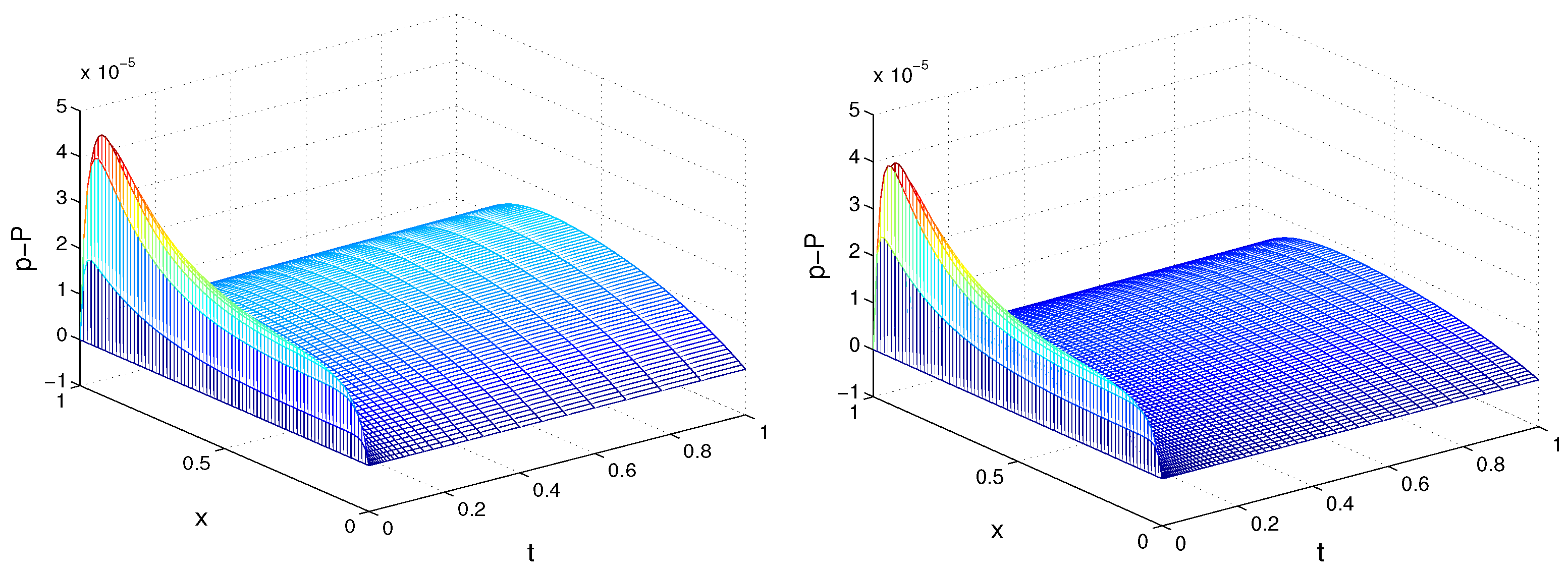
In Figure 1, we plot the error of the numerical solution for $N=I=80$, $r=2/\alpha$, $\alpha =0.2$, and $\alpha =0.5$ in the entire computational domain. As can be expected, the largest error occurs near the initial time.

6. Conclusions

In this paper, we developed a numerical scheme that is second-order accurate in time and fourth-order accurate in space for a class of time-fractional nonlinear parabolic problems. The well-posedness of the continuous problem was discussed, and a rigorous convergence analysis of the proposed scheme was carried out in the maximum norm. To handle the nonlinearity arising in the diffusion term, Newton’s iterative method was employed. In addition, a graded temporal mesh was used in order to capture the possible weak initial singularity of the solution. Numerical experiments confirm the theoretical convergence rates and demonstrate the high accuracy and efficiency of the proposed method, which requires only a small number of Newton iterations per time step.

The computational complexity is comparable to that of standard second-order schemes. The extension of the method to the same time-fractional diffusion problem in higher spatial dimensions is conceptually similar; however, the efficient implementation of the resulting high-order compact discretizations, in which high-order mixed spatial derivative terms arise during the derivation of the scheme, requires additional care.

Compared with standard second-order schemes, the proposed method attains higher spatial accuracy by using a compact discretization. Unlike semilinear schemes, it treats the quasilinear diffusion term directly, allowing greater flexibility for nonlinear problems. The method combines fourth-order spatial accuracy with graded time meshes to effectively handle weak initial singularities.

In our future work, we plan to extend the results to the higher-dimensional case and to develop a compact high-order numerical scheme for a fractional-order filtration model with double relaxation, i.e., a time-fractional pseudoparabolic problem, see, e.g., [5,38].

References

1. Bulavsky, V.M.; Bogaenko, V.A. Mathematical modeling of the fractional differential dynamics of the relaxation process of convective diffusion under conditions of planned filtration. Cybern. Syst. Anal. 2015, 51, 886–895. [Google Scholar] [CrossRef]
2. Bonforte, M.; Gualdani, M.; Ibarrondo, P. Time-fractional porous medium type equations. Sharp time decay and regularization. Calc. Var. 2026, 65, 30. [Google Scholar] [CrossRef]
3. Dar, Z.M.; Arrutselvi, M.; Muthusamy, C.; Natarajan, S.; Manzini, G. A conforming virtual element framework for the time-fractional semi-linear reaction–diffusion equation on polygonal meshes. J. Comput. Appl. Math. 2026, 476, 117100. [Google Scholar] [CrossRef]
4. De Azevedo, E.N.; Vitoreti da Silva, D.; De Souza, R.E.; Engelsberg, M. Water ingress in Y-type zeolite: Anomalous moisture-dependent transport diffusivity. Phys. Rev. E—Stat. Nonlinear Soft Matter Phys. 2006, 74, 041108. [Google Scholar] [CrossRef]
5. Khurhayrov, B.; Djiyanov, T.O.; Zokirov, M.S. Generalized relaxation fractional differential model of fluid filtration in a porous medium. Int. J. Appl. Math. 2024, 37, 119–132. [Google Scholar]
6. Mainardi, F. Fractional Calculus and Waves in Linear Viscoelasticity; Imperial College Press: London, UK, 2010. [Google Scholar]
7. Chen, H.; Stynes, M. A high order method on graded meshes for a time-fractional diffusion problem. In International Conference on Finite Difference Methods. Theory and Applications; Dimov, I., Faragó, I., Vulkov, L., Eds.; FDM 2018. Lecture Notes in Computer Science; Springer: Cham, Switzerland, 2018; Volume 11386, pp. 15–27. [Google Scholar]
8. Chen, H.; Stynes, M. Error analysis of a second-order method on fitted meshes for a time-fractional diffusion problem. J. Sci. Comput. 2019, 79, 624–647. [Google Scholar] [CrossRef]
9. Brunner, H.; Han, H.; Yin, D. The maximum principle for time-fractional diffusion equations and its application. Numer. Funct. Anal. Optim. 2015, 36, 1307–1321. [Google Scholar] [CrossRef]
10. Ding, H.; Zhang, Y. Notes on implicit finite difference approximation for time fractional diffusion equations. Comput. Math. Appl. 2011, 61, 2924–2938. [Google Scholar] [CrossRef][Green Version]
11. Kubica, A.; Yamamoto, M. Initial-boundary value problems for fractional diffusion equations with time-dependent coefficients. Fract. Calc. Appl. Anal. 2018, 21, 276–311. [Google Scholar] [CrossRef]
12. Murio, D.A. Implicit finite difference approximation for time fractional diffusion equations. Comput. Math. Appl. 2008, 56, 1138–1145. [Google Scholar] [CrossRef]
13. Nieto, J.J. Maximum principles for fractional differential equations derived from Mittag-Leffler functions. Appl. Math. Lett. 2010, 23, 1248–1251. [Google Scholar] [CrossRef]
14. Yuste, S.B.; Quintana-Murillo, J. A finite difference method with non-uniform timesteps for fractional diffusion equations. Comput. Phys. Commun. 2012, 183, 2594–2600. [Google Scholar] [CrossRef]
15. Caballero, J.; Okrasińska-Płociniczak, H.; Płociniczak, Ł.B. Barenblatt Solutions for the Time-Fractional Porous Medium Equation: Approach via Integral Equations. Preprint 2025. [Google Scholar]
16. López, B.; Okrasińska-Płociniczak, H.; Płociniczak, Ł.; Rocha, J. Time-Fractional Porous Medium Equation: Erdélyi–Kober Integral Equations, Compactly Supported Solutions, and Numerical Methods. Commun. Nonlinear Sci. Numer. Simul. 2024, 128, 107692. [Google Scholar] [CrossRef]
17. Gerasimov, D.N.; Kondratieva, V.A.; Sinkevich, O.A. An anomalous non-self-similar infiltration and fractional diffusion equation. Phys. D Nonlinear Phenom. 2010, 239, 1593–1597. [Google Scholar] [CrossRef]
18. Allen, M.; Caffarelli, L.; Vasseur, A. Porous medium flow with both a fractional potential pressure and fractional time derivative. Chin. Ann. Math. Ser. B 2017, 38, 45–82. [Google Scholar] [CrossRef]
19. Płociniczak, Ł.B. Analytical studies of a time-fractional porous medium equation. Derivation, approximation and applications. Commun. Nonlinear Sci. Numer. Simul. 2015, 24, 169–183. [Google Scholar] [CrossRef]
20. Okrasińska-Płociniczak, H.; Płociniczak, L. Second order scheme for self-similar solutions of a time-fractional porous medium equation on the half-line. Appl. Math. Comput. 2022, 424, 127033. [Google Scholar] [CrossRef]
21. Płociniczak, Ł. Numerical method for the time-fractional porous medium equation. SIAM J. Numer. Anal. 2019, 57, 638–656. [Google Scholar] [CrossRef]
22. Płociniczak, Ł.; Świtała, M. Existence and uniqueness results for a time-fractional nonlinear diffusion equation. J. Math. Anal. Appl. 2018, 462, 1425–1434. [Google Scholar] [CrossRef]
23. Zacher, R. Global strong solvability of a quasilinear subdiffusion problem. J. Evol. 2012, 12, 813–831. [Google Scholar] [CrossRef]
24. Krasnoshchok, M. Classical solutions of time-fractional quasilinear reaction-diffusion systems. Ukr. Math. J. 2025, 77, 123–138. [Google Scholar] [CrossRef]
25. Lapin, A.V.; Laitinen, E. The regularized mesh scheme to solve quasilinear parabolic equation with time-fractional derivative. Lobachevskii J. Math. 2021, 42, 1706–1714. [Google Scholar] [CrossRef]
26. Hivert, H.; Salin, F. Structure-preserving scheme for fractional nonlinear diffusion equations. arXiv 2024, arXiv:2409.18629. [Google Scholar] [CrossRef]
27. Jin, B.; Li, B.; Zhou, Z. Numerical analysis of nonlinear subdiffusion equations. SIAM J. Numer. Anal. 2018, 56, 1–23. [Google Scholar] [CrossRef]
28. Zhou, B.; Chen, X.; Li, D. Nonuniform Alikhanov linearized Galerkin finite element methods for nonlinear time-fractional parabolic equations. J. Sci. Comput. 2020, 85, 39. [Google Scholar] [CrossRef]
29. Singh, D.; Pandey, R.K.; Kumari, S. A fourth order accurate numerical method for non-linear time fractional reaction–diffusion equation on a bounded domain. Phys. D Nonlinear Phenom. 2023, 449, 133742. [Google Scholar] [CrossRef]
30. Singh, A.; Kumar, S. Higher order numerical approximations for non-linear time-fractional reaction–diffusion equations exhibiting weak initial singularity. Commun. Nonlinear Sci. Numer. Simul. 2024, 139, 1007–5704. [Google Scholar] [CrossRef]
31. Caputo, M. Models of flux in porous media with memory. Water Resour. Res. 2000, 36, 693–705. [Google Scholar] [CrossRef]
32. Kilbas, A.A.; Srivastava, H.M.; Trujillo, J.J. Theory and Applications of Fractional Differential Equations; Elsevier: Amsterdam, The Netherlands, 2006. [Google Scholar]
33. Podlubny, I. Fractional Differential Equations. An Introduction to Fractional Derivatives, Fractional Differential Equations, to Methods of Their Solution and Some of Their Applications; Academic Press: San Diego, CA, USA; Boston, MA, USA; New York, NY, USA; London, UK; Tokyo, Japan; Toronto, ON, Canada, 1999; p. 368. [Google Scholar]
34. Tatar, S.; Ulusoy, S. An inverse problem for a nonlinear diffusion equation with time-fractional derivative. J. Inverse Ill-Posed Probl. 2017, 25, 185–193. [Google Scholar] [CrossRef]
35. Samarskii, A.A. The Theory of Difference Schemes; Marcel Dekker: New York, NY, USA, 2001. [Google Scholar]
36. Alikhanov, A.A. A new difference scheme for the time fractional diffusion equation. J. Comput. Phys. 2015, 280, 424–438. [Google Scholar] [CrossRef]
37. Liao, H.-L.; McLean, W.; Zhang, J. A second-order scheme with nonuniform time steps for a linear reaction-subdiffusion problem. Commun. Comput. Phys. 2021, 30, 567–601. [Google Scholar] [CrossRef]
38. Bulavsky, V.M. Mathematical models and problems of fractional-differential dynamics of some relaxation filtration processes. Cybern. Syst. Anal. 2018, 54, 727–736. [Google Scholar] [CrossRef]
Figure 1. Error p ( x i , t n ) P i n , i = 0 , 1 , , I , n = 0 , 1 , , N of the numerical solution: I = N = 80 and α = 0.2 (left) and α = 0.5 , (right), Example 3.
Mathematics 14 00735 g001