Asymptotic Expansions for Products of Weibull Random Variables

Abstract

We derive an asymptotic expansion for the tail function of the product of $n(n\in \mathbb{N})$ independent identically distributed Weibull random variables. The coefficients of the expansion are obtained using a recursive formula arising from the Laplace method. The resulting expansion provides explicit higher-order correction terms that significantly improve the accuracy of tail approximations for large arguments. These results are useful for both theoretical analysis and practical applications involving extreme-value behavior of products of random variables. The main result of the paper shows that multiplying Weibull distributions yields so-called Weibull-type distributions. It also shows that under multiplication, the shape parameter of the Weibull distribution decreases. This implies that the product of Weibull distributions becomes more heavily tailed. The asymptotic formula for the tail function of the product of Weibull distributions involves rather complicated coefficients. To compute these coefficients, we provide MATLAB (version 9.13.0, R2022b) code. The application of the main result is illustrated with two particular examples.

1. Introduction

Products of independent random variables arise in a wide variety of areas, such as wireless communication (see, e.g., [1,2,3,4,5]), financial portfolio analysis with randomly weighted risks (see, e.g., [6,7,8,9,10]), reliability theory (see, e.g., [11,12,13,14]), and other application areas. The classical approach to analyzing such products is based on the Mellin transform. Springer’s monograph [15] and Galambos and Simonelli’s monograph [16] established the Mellin transform as a standard tool for deriving exact product distributions, and a substantial portion of the literature on product distributions continues to rely on this method. For Weibull random variables, the derivation of the product distribution can be found in the work of Lomnicki [17]. Nevertheless, the Mellin transform often leads to representations involving complicated special functions, most notably the Meijer-G function. This motivates the study of alternative approaches that focus on the asymptotic behavior of products of random variables.

Let $\xi$ be a random variable (r.v.) defined on a probability space $(\Omega ,\mathcal{F},\mathbb{P})$.

• A r.v. $\xi :\Omega \to \mathbb{R}$ is said to have the Weibull distribution with parameters $\alpha >0$ and $\beta >0$, denoted $\mathit{Weibull}(\alpha ,\beta )$, if its distribution is given by the following density function:

$$f_{\xi }\left(x\right)=\alpha \beta x^{\alpha -1}{\mathrm{e}}^{-\beta x^{\alpha }},x>0.$$

Thus the distribution function (d.f.) $F_{\xi }\left(x\right)=\mathbb{P}(\xi ⩽x)$ of such a r.v. $\xi$ is

$$F_{\xi }\left(x\right)=1-{\mathrm{e}}^{-\beta x^{\alpha }},x⩾0.$$

(1)

In the particular case $\alpha =1$, the Weibull d.f. becomes the d.f. of the exponential distribution:

$$F_{\xi }\left(x\right)=1-{\mathrm{e}}^{-\beta x},x⩾0.$$

The Weibull distribution is widely used in survival analysis due to its flexibility in modeling a range of hazard function shapes. Its shape parameter $\alpha$ allows the hazard rate

$$h_{\xi }\left(x\right)={\displaystyle \frac{f_{\xi }\left(x\right)}{1-F_{\xi }\left(x\right)}}=\alpha \beta x^{\alpha -1}$$

to increase, decrease, or remain constant over time. This makes the Weibull model suitable for analyzing both medical survival data and reliability or failure-time data. The distribution handles censored observations well, which are common in survival studies.

In addition to survival and failure analysis [18,19], the Weibull distribution is also considered in life insurance as a model of the lifetime distribution, in risk analysis as a model of the claim size distribution [20,21], in economics and financial mathematics as a model of asset returns distribution or income distribution [22,23,24], in the coal industry for the description of statistical regularities of particle sizes [25,26], in the queueing theory for the description of waiting or service time [27,28], in radio engineering meteorology, hydrology, and other fields; see, e.g., [18,19,29,30,31].

If the parameter $\alpha \in (0,1)$, then Weibull’s distribution $F_{\xi }\left(x\right)=\left(1-{\mathrm{e}}^{-\beta x^{\alpha }}\right){\mathbb{I}}_{[0,\infty )}\left(x\right)$ belongs to the heavy tails distribution class $\mathcal{H}$, because

$$\underset{[0,\infty )}{\int }{\mathrm{e}}^{\delta x}\mathrm{d}{F}_{\xi }\left(x\right)=\infty$$

for all $\delta >0$. When $\alpha >1$, Weibull’s distribution is light-tailed (equivalently, belongs to the class ${\mathcal{H}}^c$), because

$$\begin{array}{c}\hfill \underset{[0,\infty )}{\int }{\mathrm{e}}^{\delta x}\mathrm{d}{F}_{\xi }\left(x\right)<\infty \end{array}$$

(2)

for all $\delta >0$. In the intermediate case $\alpha =1$, Weibull’s distribution becomes exponential, which is also light-tailed because (2) holds for all $\delta \in (0,\beta )$.

For any independent r.v.s $\xi :\Omega \to \mathbb{R}$ and $\eta :\Omega \to \mathbb{R}$, the d.f. of $\xi \eta$ is expressed as the product-convolution of d.f.s $F_{\xi }$ and $F_{\eta }$, i.e.,

$$\begin{array}{cc}\hfill \mathbb{P}(\xi \eta ⩽x)& =F_{\xi }\otimes F_{\eta }\left(x\right)=\underset{(-\infty ,0)}{\int }\left(1-F_{\xi }\left({\displaystyle \frac{x}{y}}-0\right)\right)\mathrm{d}{F}_{\eta }\left(y\right)\hfill \\ & +\underset{(0,\infty )}{\int }{F}_{\xi }\left({\displaystyle \frac{x}{y}}\right)\mathrm{d}{F}_{\eta }\left(y\right)+\left(F_{\eta }\left(0\right)-F_{\eta }(0-)\right){\mathbb{I}}_{[0,\infty )}\left(x\right).\hfill \end{array}$$

In most cases, we consider the situation where one variable, say $\eta$, is non-negative and nondegenerate at zero, i.e., $F_{\eta }(0-)=0, F_{\eta }\left(0\right)<1$. In this case,

$$F_{\xi }\otimes F_{\eta }\left(x\right)=\underset{(0,\infty )}{\int }{F}_{\xi }\left({\displaystyle \frac{x}{y}}\right)\mathrm{d}{F}_{\eta }\left(y\right)+F_{\eta }\left(0\right){\mathbb{I}}_{[0,\infty )}\left(x\right)$$

and

$$\overline{F_{\xi }\otimes F_{\eta }}\left(x\right)=\underset{(0,\infty )}{\int }{\overline{F}}_{\xi }\left({\displaystyle \frac{x}{y}}\right)\mathrm{d}{F}_{\eta }\left(y\right),x>0.$$

In this paper, we investigate the product of n independent identically distributed (i.i.d.) Weibull r.v.s. The derived asymptotic Formula (6) for the tail of the product distribution implies, among other results, that the product of independent Weibull random variables exhibits heavier tails than the initial distribution. This phenomenon occurs because the shape parameter of the Weibull distribution decreases under multiplication: after n independent products, an initial shape parameter $\alpha$ is reduced to $\alpha /n$. For example, if the initial value of the parameter is $\alpha =10$ (light-tailed case), then the product of eleven independent Weibull-distributed variables yields a distribution ${\Pi }_{11}$ with the following leading tail term:

$${\displaystyle \frac{{\left(2\pi \beta \right)}^5}{\sqrt{11}}}{\mathrm{e}}^{-10\beta x^{10/11}}{x}^{50/11}.$$

Hence, the resulting distribution ${\Pi }_{11}$ is already heavy-tailed since

$$\underset{[0,\infty )}{\int }{\mathrm{e}}^{\delta x}\mathrm{d}{\Pi }_{11}\left(x\right)=1+\delta \underset{0}{\overset{\infty }{\int }}{\mathrm{e}}^{\delta x}{\Pi }_{11}\left(x\right)\mathrm{d}x=\infty$$

for all $\delta$ > 0. The product of identically distributed Weibull random variables does not itself follow a Weibull distribution; nevertheless, its tail behavior retains a closely related structure in some sense. A similar weighting of the tails of distributions when multiplying them is also observed in [32,33,34,35,36].

The remainder of the paper is organized as follows. In Section 2, we discuss known results related to the problem under consideration. In Section 3, we state the main results of the paper. Section 4 is devoted to a collection of auxiliary statements. A detailed proof of the main theorem of the paper is given in Section 5. Section 6 and Section 7 are intended to show how to apply the resulting asymptotic formula to particular cases. In Section 8, we provide a brief review of the main result and discuss its significance. Lastly, we present the MATLAB code for computations of our recursive formula.

2. Known Results

Arendarczyk and Dȩbicki derived an asymptotic formula for the product of two distributions with Weibull-type tails. Namely, in [33] [Lemma 2.1], the following statement is presented.

Proposition 1. 

Let ${\xi }_1$ and ${\xi }_2$ be two independent r.v.s, such that

$$\mathbb{P}\left({\xi }_i>x\right)\underset{x\to \infty }{\sim }{c}_i{x}^{{\gamma }_i}exp\left\{-{\beta }_i{x}^{{\alpha }_i}\right\},i=1,2,$$

for some positive ${\alpha }_1,{\alpha }_2,{\beta }_1,{\beta }_2,c_1,c_2$ and real ${\gamma }_1,{\gamma }_2$. Then

$$\mathbb{P}\left({\xi }_1{\xi }_2>x\right)\underset{x\to \infty }{\sim }c{x}^{\gamma }exp\left\{-\beta x^{\alpha }\right\},$$

where   

$$\begin{array}{cc}\hfill \alpha & ={\displaystyle \frac{{\alpha }_1{\alpha }_2}{{\alpha }_1+{\alpha }_2}},\gamma ={\displaystyle \frac{{\alpha }_1{\alpha }_2+2{\alpha }_1{\gamma }_2+2{\alpha }_2{\gamma }_1}{2({\alpha }_1+{\alpha }_2)}},\hfill \\ \hfill \beta & ={\beta }_1^{{\displaystyle \frac{{\alpha }_2}{{\alpha }_1+{\alpha }_2}}}{\beta }_2^{{\displaystyle \frac{{\alpha }_1}{{\alpha }_1+{\alpha }_2}}}\left({\left({\displaystyle \frac{{\alpha }_1}{{\alpha }_2}}\right)}^{{\displaystyle \frac{{\alpha }_2}{{\alpha }_1+{\alpha }_2}}}+{\left({\displaystyle \frac{{\alpha }_2}{{\alpha }_1}}\right)}^{{\displaystyle \frac{{\alpha }_1}{{\alpha }_1+{\alpha }_2}}}\right),\hfill \\ \hfill c& ={\displaystyle \frac{c_1{c}_2\sqrt{2\pi }}{\sqrt{{\alpha }_1+{\alpha }_2}}}{\left({\alpha }_1{\beta }_1\right)}^{{\displaystyle \frac{{\alpha }_2-2{\gamma }_1+2{\gamma }_2}{2({\alpha }_1+{\alpha }_2)}}}{\left({\alpha }_2{\beta }_2\right)}^{{\displaystyle \frac{{\alpha }_1-2{\gamma }_2+2{\gamma }_1}{2({\alpha }_1+{\alpha }_2)}}}.\hfill \end{array}$$

In [37] [Theorem 1], i.i.d. random variables ${\xi }_1,{\xi }_2,\dots ,{\xi }_n$ with standard exponential distribution $\mathbb{P}({\xi }_1>x)={\mathrm{e}}^{-x},x⩾0,$ are considered. It is derived that

$$\mathbb{P}\left(\prod _{i=1}^n{\xi }_i>x\right)={\displaystyle \frac{{\left(2\pi \right)}^{(n-1)/2}}{\sqrt{n}}}{x}^{(n-1)/2n}exp\left\{-n{x}^{1/n}\right\}{g}_n\left(x\right),n\in \mathbb{N},$$

for some functions $g_n\left(x\right)$, such that

$$\underset{x\to \infty }{lim}{g}_n\left(x\right)=1.$$

In [38] [Equality (9)], it is observed that by multiplying n i.i.d. Weibull-type distributions ${\xi }_1,{\xi }_2,\dots ,{\xi }_n$ with tails

$$\mathbb{P}({\xi }_1>x)\underset{x\to \infty }{\sim }c{x}^{\gamma }exp\{-\beta x^{\alpha }\},\alpha >0,\beta >0,c>0,\gamma \in \mathbb{R},$$

we obtain that

$$\begin{array}{c}\hfill \mathbb{P}\left(\prod _{i=1}^n{\xi }_i>x\right)\underset{x\to \infty }{\sim }{\displaystyle \frac{c^n}{\sqrt{n}}}{\left(2\pi \beta \right)}^{{\displaystyle \frac{n-1}{2}}}{x}^{(2n\gamma +(n-1\left)\alpha \right)/2n}exp\left\{-n\beta x^{\alpha /n}\right\}.\end{array}$$

(3)

In the case of the “free” Weibull distribution (1), equality (3) implies that for all $n\in \mathbb{N}$,

$$\begin{array}{c}\hfill \mathbb{P}\left(\prod _{i=1}^n{\xi }_i>x\right)\underset{x\to \infty }{\sim }{\displaystyle \frac{{\left(2\pi \beta \right)}^{\frac{n-1}{2}}}{\sqrt{n}}}{x}^{{\displaystyle \frac{\alpha (n-1)}{2n}}}exp\left\{-n\beta x^{\alpha /n}\right\}.\end{array}$$

(4)

In [36], the asymptotic formula with the remainder term is derived for the product of gamma distributions. By using the Laplace method, the following statement is derived.

Proposition 2. 

Let ${\xi }_1,{\xi }_2,\dots ,{\xi }_n$ be i.i.d. r.v.s such that for each k,

$$\mathbb{P}\left({\xi }_k>x\right)={\displaystyle \frac{{\beta }^{\alpha }}{\Gamma \left(\alpha \right)}}\underset{x}{\overset{\infty }{\int }}{y}^{\alpha -1}{\mathrm{e}}^{-\beta y}\mathrm{d}y\underset{x\to \infty }{\sim }{\displaystyle \frac{{\beta }^{\alpha -1}}{\Gamma \left(\alpha \right)}}{x}^{\alpha -1}{\mathrm{e}}^{-\beta x},$$

where $\alpha >0$, $\beta >0$ are parameters, and the symbol Γ denotes the classical gamma function, i.e.,

$$\Gamma \left(\alpha \right)=\underset{0}{\overset{\infty }{\int }}{u}^{\alpha -1}{\mathrm{e}}^{-y}\mathrm{d}y.$$

Then

$$\begin{array}{cc}\hfill {\overline{F}}_{{\xi }_1{\xi }_2,\dots ,{\xi }_n}\left(x\right)& ={\displaystyle \frac{{\left(2\pi \right)}^{(n-1)/2}}{\sqrt{n}}}{\displaystyle \frac{{\beta }^{n(\alpha -1)+(n-1)/2}}{{\Gamma }^n\left(\alpha \right)}}{x}^{\alpha -{\displaystyle \frac{n+1}{2n}}}exp\left\{-n\beta x^{1/n}\right\}\hfill \\ \hfill & \times \left(1+{\displaystyle \frac{\alpha -1-S_n}{\beta x^{1/n}}}+O\left(x^{-3/\left(2n\right)}\right)\right),\hfill \end{array}$$

where $S_1=0$,    

$$S_n=\sum _{k=2}^n{\displaystyle \frac{k(k-1)-11}{24k(k-1)}},n⩾2,$$

(5)

and the constant in the symbol O depends on $\alpha ,\beta ,n$, but does not depend on x.

We continue our investigation of the tails of products of i.i.d. r.v.s. Using the Laplace method, we derive an asymptotic expansion for the tail distribution, including a “free” Weibull r.v. as a generator. It is obvious that the main asymptotic Formula (6) is a direct generalization of the asymptotic relation (4).

3. Main Results

We state the main theorem in terms of the Laplace method constants $c_{·,·,·}$. Explicit representation of these constants is omitted at this stage, as the asymptotic Formula (6) involves recursively defined coefficients ${\mathcal{D}}_{·,·}$. For practical purposes, explicit expressions of the resulting tail asymptotics are given in the subsequent corollaries, where the cases $N=2$ and $N=4$ are derived.

Theorem 1. 

Let ${\xi }_1,{\xi }_2,\dots$ be i.i.d. r.v.s. such that for each l $\in \mathbb{N}$, ${\xi }_l$ is distributed according to $\mathit{Weibull}\left(\alpha ,\beta \right)$ law. Then for the product ${\Pi }_n:={\prod }_{l=1}^n{\xi }_l$, we have

$$\begin{array}{c}\hfill {\overline{F}}_{{\Pi }_n}\left(x\right)={\displaystyle \frac{{\left(2\pi \beta \right)}^{\frac{n-1}{2}}}{\sqrt{n}}}{e}^{-n\beta x^{\alpha /n}}{x}^{\alpha {\displaystyle \frac{n-1}{2n}}}\left(1+\sum _{k=1}^{\lfloor N/2\rfloor }{\beta }^{-k}{x}^{-\frac{\alpha k}{n}}{\mathcal{D}}_{2k,n}+O\left(x^{-\alpha {\displaystyle \frac{N+1}{2n}}}\right)\right),\end{array}$$

(6)

where $N\in {\mathbb{N}}_0=\{0,1,2,\dots \}$, ${\mathcal{D}}_{0,n}=1$ for $n\in \mathbb{N},{\mathcal{D}}_{2j,1}=0$ for $j\in \{1,\dots ,\lfloor N/2\rfloor \}$, and

$${\mathcal{D}}_{2k,n}:=\sum _{j=0}^k{\mathcal{D}}_{2j,n-1}{\displaystyle \frac{\Gamma \left(k-j+\frac{1}{2}\right)}{\sqrt{\pi }}}{\displaystyle \frac{c_{2(k-j),2j,n}}{c_{0,0,n}}}\mathit{for}k\in \{1,\dots ,\lfloor N/2\rfloor \},$$

(7)

and the constants with three indices $c_{·,·,·}$ are found using a special algorithm. The indices in the constants $c_{·,·,·}$ label, respectively, the summation order, the index of the approximated integral, and the number of random variables in the product.

Remark 1. 

The coefficients ${\mathcal{D}}_{·,·}$ and $c_{·,·,·}$ appearing in the asymptotic expansion (6) are determined via the procedures outlined in Algorithm 1. Procedure I computes the base coefficients $c_{·}$ using Wojdylo’s formula. Procedure II computes Taylor coefficients for integrals in (20) and uses procedure I to obtain $c_{·,·,·}$. Finally, Procedure III applies the recursive Formula (7) to obtain the final coefficients $\left\{{\mathcal{D}}_{2k,n}\right\}$ for any product length n. Note that loop indices and intermediate symbols, such as s, ℓ, r, are dummy variables used locally within the corresponding loops.

The detailed MATLAB code for calculating the coefficients $c_{·,·,·}$ and ${\mathcal{D}}_{·,·}$ is presented in Appendix A. Using Theorem 1 for small values of N, we obtain the following explicit formulas.

Corollary 1. 

For $N=2$, the asymptotic expansion in Theorem 1 reduces to

$$\begin{array}{c}\hfill {\overline{F}}_{{\Pi }_n}\left(x\right)={\displaystyle \frac{{\left(2\pi \beta \right)}^{\frac{n-1}{2}}}{\sqrt{n}}}{\mathrm{e}}^{-n\beta x^{\alpha /n}}{x}^{\alpha {\displaystyle \frac{n-1}{2n}}}\left(1+{\beta }^{-1}{x}^{-\frac{\alpha }{n}}{\mathcal{D}}_{2,n}+O\left(x^{-\frac{3\alpha }{2n}}\right)\right),\end{array}$$

where $n\in \mathbb{N}$, and

$${\mathcal{D}}_{2,n}={\displaystyle \frac{1}{24}}\left(12-n-{\displaystyle \frac{11}{n}}\right).$$

(8)

Corollary 2. 

For $N=4$, the tail function of product ${\Pi }_n$, $n\in \mathbb{N}$, reduces to

$$\begin{array}{c}\hfill {\overline{F}}_{{\Pi }_n}\left(x\right)={\displaystyle \frac{{\left(2\pi \beta \right)}^{\frac{n-1}{2}}}{\sqrt{n}}}{\mathrm{e}}^{-n\beta x^{\alpha /n}}{x}^{\alpha {\displaystyle \frac{n-1}{2n}}}\left(1+{\beta }^{-1}{x}^{-\frac{\alpha }{n}}{\mathcal{D}}_{2,n}+{\beta }^{-2}{x}^{-\frac{2\alpha }{n}}{\mathcal{D}}_{4,n}+O\left(x^{-\frac{5\alpha }{2n}}\right)\right),\end{array}$$

where ${\mathcal{D}}_{2,n}$ is defined in (8), and

$$\begin{array}{cc}\hfill {\mathcal{D}}_{4,n}& ={\displaystyle \frac{1}{1152}}\left(n^2-24n+3262-120\sum _{k=1}^n{\displaystyle \frac{1}{k}}-1320\sum _{k=1}^n{\displaystyle \frac{1}{k^2}}-{\displaystyle \frac{3888}{n}}+{\displaystyle \frac{2089}{n^2}}\right).\hfill \end{array}$$

(9)

Algorithm 1 Computation of coefficients ${\mathcal{D}}_{2k,n}$.

Require:  N, n Ensure:  Coefficients $\left\{{\mathcal{D}}_{2k,n}\right\}$    1: $K\leftarrow \lfloor N/2\rfloor +1$             ▹ row count of coefficient $\left\{{\mathcal{D}}_{2k,n}\right\}$ table    2: Initialize ${\mathcal{D}}_{0,1}\leftarrow 1$        3: Procedure I: Coefficient computation by Wojdylo’s formula    4: for $s=0$ to N do    5:       Obtain Taylor coefficients ${\left\{a_i\right\}}_{i=0}^s$, ${\left\{b_i\right\}}_{i=0}^s$    6:       Compute Bell coefficients ${\mathcal{C}}_{n,k}$ using recursion (18)    7:       Obtain scaled coefficients $c_s^{*}$ from (17)    8:       Compute coefficients $c_s$ using (16)    9: end for  10: Procedure II: Integral coefficients from (20)  11: for all triples $(2k,2j,n)$ do  12:        Construct Taylor coefficients $\left\{a_{2k}^{\left(n\right)}\right\}$, $\left\{b_{2k}^{\left(n\right)}\right\}$  13:        Define $c_{2k,2j,n}\leftarrow c_{2k}$ via Procedure I  14: end for  15: Procedure III: Final coefficient recursion  16: for $\mathsf{\ell }=2$ to n do  17:       Compute normalization constant $c_{0,0,\mathsf{\ell }}$  18:       for $r=1$ to $K-1$ do  19:             Compute ${\mathcal{D}}_{2r,\mathsf{\ell }}$ using recursion (7)  20:     end for  21: end for  22: return$\left\{{\mathcal{D}}_{2k,n}\right\}$

Remark 2. 

In the Formula (9), we give an exact expression for the coefficient ${\mathcal{D}}_{4,n}$ for a fixed number of product terms n. This expression is obtained by solving the recursive Equation (21) below. The given expression includes two harmonic sums

$$H_n^{\left(1\right)}=\sum _{k=1}^n{\displaystyle \frac{1}{k}}\mathrm{and}{H}_n^{\left(2\right)}=\sum _{k=1}^n{\displaystyle \frac{1}{k^2}}.$$

If n is large enough, then instead of the exact expression, we can use approximations obtained from the classical Euler–Maclaurin summation formula. According to such a formula

$$\begin{array}{c}{H}_n^{\left(1\right)}=\log n+\gamma +{\displaystyle \frac{1}{2n}}-\sum _{m=1}^{\infty }{\displaystyle \frac{B_{2m}}{2m{n}^{2m}}}\approx logn+\gamma +{\displaystyle \frac{1}{2n}}-{\displaystyle \frac{1}{12n^2}},\\ H_n^{\left(2\right)}={\displaystyle \frac{{\pi }^2}{6}}-{\displaystyle \frac{1}{n}}+{\displaystyle \frac{1}{2n^2}}-\sum _{m=1}^{\infty }{\displaystyle \frac{B_{2m}}{n^{2m+1}}}\approx {\displaystyle \frac{{\pi }^2}{6}}-{\displaystyle \frac{1}{n}}+{\displaystyle \frac{1}{2n^2}}-{\displaystyle \frac{1}{6n^3}},\end{array}$$

where $\gamma$ is the Euler–Masheroni constant and $B_{2m},m\in \mathbb{N},$ are the Bernoulli numbers.

The statements of Corollaries 1 and 2 follow directly from the main Theorem 1, and the derivation of the expressions (8) and (9) is discussed in Section 6.

4. Auxiliary Lemmas

To prove the main theorem, we first present some auxiliary lemmas. We begin with Watson’s lemma; for proofs and detailed discussions, see, e.g., [39], [40] [Chapter I], [41] [Theorem 3.1 on page 71], and [42] [Chapter 2].

Lemma 1. 

Let $\phi \left(t\right)=t^{\lambda }g\left(t\right)$, where $g\in C^{\infty }[0,\delta ]$ for some $\delta >0$, $g\left(0\right)\ne 0$, and $\lambda >-1$. In addition, suppose $\left|\phi \left(t\right)\right|<K{\mathrm{e}}^{bt}$ for all $t>0$ with constants K and b independent of t. Then

$$\left|\underset{0}{\overset{\infty }{\int }}\phi \left(t\right){\mathrm{e}}^{-xt}\mathrm{d}t\right|<\infty$$

for sufficiently large x, and for all $N\in {\mathbb{N}}_0$,

$$\underset{0}{\overset{\infty }{\int }}\phi \left(t\right){\mathrm{e}}^{-xt}\mathrm{d}t=\underset{0}{\overset{\infty }{\int }}{t}^{\lambda }g\left(t\right){\mathrm{e}}^{-xt}\mathrm{d}t=\sum _{k=0}^N{\displaystyle \frac{g^{\left(k\right)}\left(0\right)\Gamma (\lambda +k+1)}{k!x^{\lambda +k+1}}}+O\left(x^{-(\lambda +N+2)}\right)$$

as $x\to \infty$, where the bounding constant in the symbol O does not depend on x.

We next recall the Laplace method. The result may be obtained by applying Watson’s Lemma 1 to a real integral of a special form. A complete proof is given by Wong [40] (see Theorem 1 in Chapter II). Historically, this formulation of the Laplace method traces back to the work of Erdélyi [43]. Further developments and related analysis can be found in the classical works [44,45,46,47].

Lemma 2. 

Let h and g be two real functions defined on an interval $[a,b)$, where b can be finite or infinite, satisfying the following properties:

(i)

For all $N\in \mathbb{N}$, as $z\downarrow a$,

$$\begin{array}{cc}\hfill h\left(z\right)& =h\left(a\right)+\sum _{k=0}^N{a}_k{(z-a)}^{k+\mu }+o\left({(z-a)}^{N+\mu }\right),\hfill \\ \hfill g\left(z\right)& =\sum _{k=0}^N{b}_k{(z-a)}^{k+\nu -1}+o\left({(z-a)}^{N+\nu -1}\right),\hfill \\ \hfill h^{\prime }\left(z\right)& =\sum _{k=0}^N(k+\mu )a_k{(z-a)}^{k+\mu -1}+o\left({(z-a)}^{N+\mu -1}\right),\hfill \end{array}$$

where $a_0\ne 0$, $b_0\ne 0$, $\mu >0$, and $\nu >0$.

(ii)

$h\left(z\right)>h\left(a\right)$ for all $z\in (a,b)$, and

$$\underset{z\in [a+\delta ,b)}{inf}\left(h\left(z\right)-h\left(a\right)\right)>0\mathit{for}\mathit{all}\delta >0.$$

(iii)

$h^{\prime }$ and g are continuous in a neighborhood of a.

If the integral

$$\underset{a}{\overset{b}{\int }}g\left(z\right)e^{-xh\left(z\right)}\mathrm{d}z$$

converges absolutely for all sufficiently large x, then for each $N\in {\mathbb{N}}_0$,

$$\underset{a}{\overset{b}{\int }}g\left(z\right){\mathrm{e}}^{-xh\left(z\right)}\mathrm{d}z={\mathrm{e}}^{-xh\left(a\right)}\left(\sum _{k=0}^N\Gamma \left({\displaystyle \frac{k+\nu }{\mu }}\right)c_k{x}^{-(k+\nu )/\mu }+O\left(x^{-(N+\nu +1)/\mu }\right)\right),$$

(10)

where the coefficients $c_k$ can be expressed in terms of $a_k$ and $b_k$. A detailed algorithm for finding the coefficients $c_k$ is described in Lemma 4.

Although the previous lemma establishes a general Laplace expansion, the analysis of products of i.i.d Weibull r.v.s leads to integrals of the form

$$\underset{0}{\overset{\infty }{\int }}{u}^{{\displaystyle \frac{2l+1-m}{2m}}}{\mathrm{e}}^{-x(u+m{u}^{-1/m})}\mathrm{d}u,$$

where $l\in {\mathbb{N}}_0$ and $m\in \mathbb{N}$.

It is important to note that when applying the Laplace method to the integral of this type, all odd-order coefficients in the resulting expansion vanish. We formalize this observation for the considered integrals in the following lemma.

Lemma 3. 

For all $l\in {\mathbb{N}}_0$, $m\in \mathbb{N}$, and $N\in {\mathbb{N}}_0$,

$$\begin{array}{c}\hfill \underset{0}{\overset{\infty }{\int }}{u}^{{\displaystyle \frac{2l+1-m}{2m}}}{\mathrm{e}}^{-x(u+m{u}^{-1/m})}\mathrm{d}u=2{\mathrm{e}}^{-x(m+1)}\left(\sum _{k=0}^{\lfloor N/2\rfloor }\Gamma \left(k+{\displaystyle \frac{1}{2}}\right)d_{2k}{x}^{-(k+1/2)}+O\left(x^{-(N+2)/2}\right)\right),\end{array}$$

where constant in symbol O does not depend on x, and $\{d_{2k},k=0,1,\dots \}$ is a sequence of coefficients possibly dependent on l and m.

Remark 3. 

The lemma, in fact, states that the considered integral is expressed in the degrees

$$x^{-1/2},x^{-3/2},x^{-5/2},x^{-7/2},\dots .$$

Meanwhile, the degrees

$$x^{-1},x^{-2},x^{-3},x^{-4},\dots$$

do not participate in the asymptotic expression of the integral.

Proof. 

Let us write

$$\begin{array}{cc}\hfill \mathcal{I}\left(x\right)& =\underset{0}{\overset{\infty }{\int }}{u}^{{\displaystyle \frac{2l+1-m}{2m}}}{\mathrm{e}}^{-x(u+m{u}^{-1/m})}\mathrm{d}u=\left(\underset{0}{\overset{1}{\int }}+\underset{1}{\overset{\infty }{\int }}\right)u^{{\displaystyle \frac{2l+1-m}{2m}}}{\mathrm{e}}^{-x(u+m{u}^{-1/m})}\mathrm{d}u\hfill \\ \hfill & :={\mathcal{I}}_1\left(x\right)+{\mathcal{I}}_2\left(x\right).\hfill \end{array}$$

First, consider the second integral

$${\mathcal{I}}_2\left(x\right)=\underset{1}{\overset{\infty }{\int }}{u}^{{\displaystyle \frac{2l+1-m}{2m}}}{\mathrm{e}}^{-x(u+m{u}^{-1/m})}\mathrm{d}u.$$

To apply Watson’s lemma, we make the variable change

$${\phi }_1\left(u\right)=u+m{u}^{-1/m}-(1+m)=t.$$

(11)

Since the function ${\phi }_1$ increases on the interval $\left[1,\infty \right]$, there exists an inverse function ${\phi }_1^{-1}$. Therefore, from (11), we have

$$u={\phi }_1^{-1}\left(t\right),t⩾0,$$

and

$$\begin{array}{cc}\hfill {\mathcal{I}}_2\left(x\right)& ={\mathrm{e}}^{-x(m+1)}\underset{0}{\overset{\infty }{\int }}{\mathrm{e}}^{-xt}{t}^{-1/2}{g}_1\left(t\right)\mathrm{d}t\hfill \end{array}$$

with

$$g_1\left(t\right)=t^{1/2}{\left({\phi }_1^{-1}\left(t\right)\right)}^{{\displaystyle \frac{2l+1-m}{2m}}}{\left({\phi }_1^{-1}\left(t\right)\right)}^{\prime }.$$

Since the function

$$u+{\displaystyle \frac{m}{u^{1/m}}}-(1+m)-logu,u⩾1,$$

eventually increases in u, we get that for $t>0$,

$$\begin{array}{c}\hfill \left|{\phi }_1^{-1}\left(t\right)\right|⩽K_0{\mathrm{e}}^{L_{0}t}\mathrm{and}\left|g_1\left(t\right)\right|⩽K_1{\mathrm{e}}^{L_{1}t}\end{array}$$

(12)

with some positive $K_0,K_1,L_0,L_1$ independent of t.

• If $1⩽u<2$, then

$${\phi }_1\left(u\right)={\displaystyle \frac{1}{2}}{\displaystyle \frac{m+1}{m}}{(u-1)}^2+\sum _{r=3}^{\infty }{(u-1)}^r{\displaystyle \frac{1}{r!m^r}}\prod _{l=1}^{r-1}(m+l).$$

Due to Lagrange’s inversion formula,

$${\phi }_1^{-1}\left(t\right)=1+\sum _{k=1}^{\infty }{a}_{mr}{t}^{r/2}:=1+\Psi \left(\sqrt{t}\right),$$

(13)

where $t\in \left[0,\delta \right]$ for some positive $\delta$, and $\{a_{mr},r\in \mathbb{N}\}$ is a sequence of positive coefficients such that

$$\begin{array}{c}\hfill a_{m1}=\sqrt{{\displaystyle \frac{2m}{m+1}}},a_{m2}={\displaystyle \frac{2m+1}{3(m+1)}},a_{m3}={\displaystyle \frac{(m+2)(2m+1)}{36}}\sqrt{{\displaystyle \frac{2}{m{(m+1)}^3}}}.\end{array}$$

Therefore, for $t\in [0,\delta ]$, we can write

$$\begin{array}{cc}\hfill g_1\left(t\right)& =t^{1/2}{\left(1+\Psi \left(\sqrt{t}\right)\right)}^{{\displaystyle \frac{2l+1-m}{2m}}}{\left(\Psi \left(\sqrt{t}\right)\right)}^{\prime }\hfill \\ \hfill & ={\displaystyle \frac{1}{2}}{\left(1+\Psi \left(\sqrt{t}\right)\right)}^{{\displaystyle \frac{2l+1-m}{2m}}}\psi \left(\sqrt{t}\right),\hfill \end{array}$$

where

$$\begin{array}{cc}\hfill & \psi \left(\sqrt{t}\right)=\sum _{r=1}^{\infty }r{a}_{mr}{\left(\sqrt{t}\right)}^{r-1}=a_{m1}+\sum _{r=2}^{\infty }r{a}_{mr}{t}^{(r-1)/2}.\hfill \end{array}$$

(14)

For the integral ${\mathcal{I}}_1\left(x\right)$, we get that

$${\mathcal{I}}_1\left(x\right)=\underset{-1}{\overset{0}{\int }}{(-v)}^{{\displaystyle \frac{2l+1-m}{2m}}}{\mathrm{e}}^{-x((-v)-m{v}^{-1/m})}\mathrm{d}v.$$

After the change of variables

$${\phi }_2(-v)=-v-m{v}^{-1/m}-(1+m)=t,$$

we get that

$${\mathcal{I}}_1\left(x\right)={\mathrm{e}}^{-x(m+1)}\underset{0}{\overset{\infty }{\int }}{\mathrm{e}}^{-xt}{t}^{-1/2}{g}_2\left(t\right)\mathrm{d}t,$$

where

$$g_2\left(t\right)=t^{1/2}{\left({\phi }_2^{-1}\left(t\right)\right)}^{{\displaystyle \frac{2l+1-m}{2m}}}{\left({\phi }_2^{-1}\left(t\right)\right)}^{\prime },$$

and ${\phi }_2^{-1}\left(t\right)$ is the inverse function for ${\phi }_2(-v)$, i.e.,

$$(-v)={\phi }_2^{-1}\left(t\right),v=-{\phi }_2^{-1}\left(t\right).$$

Similarly to the function $g_1$, for the function $g_2$, we can obtain that

$$\begin{array}{c}\hfill |g_2\left(t\right)|⩽K_2{\mathrm{e}}^{L_{2}t},t>0,\end{array}$$

(15)

with some $K_2>0$ and $L_2>0$ independent of t. According to the Lagrange inversion formula,

$$\begin{array}{cc}\hfill {\phi }_2^{-1}\left(t\right)& =1-\sqrt{{\displaystyle \frac{2m}{m+1}}}{t}^{1/2}+{\displaystyle \frac{2m+1}{3(m+1)}}t-{\displaystyle \frac{(m+2)(2m+1)}{36}}\sqrt{{\displaystyle \frac{2}{m{(m+1)}^3}}}{t}^{3/2}+\cdots ,\hfill \\ \hfill & =1+\Psi (-\sqrt{t}),\hfill \end{array}$$

where $t\in [0,\delta ]$, and the function $\Psi$ is defined in (13). In addition, for $t\in [0,\delta ]$, we have

$$\begin{array}{cc}\hfill {\left({\phi }_2^{-1}\left(t\right)\right)}^{\prime }& ={\left(\Psi (-\sqrt{t})\right)}^{\prime }=-{\displaystyle \frac{t^{-1/2}}{2}}\left(a_{m1}-2a_{m2}{t}^{1/2}+3a_{m3}t-4a_{m4}{t}^{3/2}+\cdots \right)\hfill \\ \hfill & =-{\displaystyle \frac{t^{-1/2}}{2}}\psi (-\sqrt{t})\hfill \end{array}$$

with function $\psi$ defined in (14).

• Consequently,

$$g_2\left(t\right)={\displaystyle \frac{1}{2}}{\left(1+\Psi (-\sqrt{t})\right)}^{{\displaystyle \frac{2l+1-m}{2m}}}\psi \left(-\sqrt{t}\right)$$

for $t\in [0,\delta ]$.

• By adding ${\mathcal{I}}_1\left(x\right)$ and ${\mathcal{I}}_2\left(x\right)$, we obtain that

$$\mathcal{I}\left(x\right)={\mathrm{e}}^{-x(m+1)}\underset{0}{\overset{\infty }{\int }}{\mathrm{e}}^{-xt}{t}^{-1/2}\left(g_1\left(t\right)+g_2\left(t\right)\right)\mathrm{d}t.$$

Due to inequalities (12) and (15), the function $g=g_1+g_2$ satisfies the estimate

$$\left|g\left(t\right)\right|⩽K_3{\mathrm{e}}^{L_{3}t},t>0,$$

with some $K_3>0$ and $L_3>0$ independent of t.

• If $t\in \left[0,\delta \right]$, then

$$g\left(t\right)={\displaystyle \frac{1}{2}}{\left(1+\Psi \left(\sqrt{t}\right)\right)}^{{\displaystyle \frac{2l+1-m}{2m}}}\psi \left(\sqrt{t}\right)+{\displaystyle \frac{1}{2}}{\left(1+\Psi (-\sqrt{t})\right)}^{{\displaystyle \frac{2l+1-m}{2m}}}\psi (-\sqrt{t}).$$

Consequently, for $t\in [0,\delta ]$, the function g has the representation

$$g\left(t\right)=\sum _{k=0}^{\infty }{d}_{2k}{t}^k,$$

where $\{d_{2k},k\in {\mathbb{N}}_0\}$ is a sequence of real numbers such that $d_0=a_{m1}>0$. By Watson’s Lemma 1, the asymptotic formula of Lemma 3 holds.    □

Remark 4. 

From the proof above, we can see that the statement analogous to Lemma 3 is also valid in a more general case. It is only necessary that the function in the exponent becomes symmetric with respect to the minimum point after a suitable transformation, and the function near the exponent becomes even after a change of variables. It is quite difficult to strictly describe the initial conditions for this to happen, so we only consider integrals of the form we need. A similar situation occurs for complex integrals; the only important thing is that the minimum point of the function under the exponent is attained in the integration interval; see, e.g., formulation of Theorem 7.1 on page 127 of [41].

After establishing that all odd-order coefficients in our expansion vanish, it remains to determine the remaining even-order coefficients in the asymptotic Formula (10). Wong [40] provided explicit forms of the first three coefficients:

$$\begin{array}{cc}\hfill c_0& ={\displaystyle \frac{b_0}{\mu a_0^{\nu /\mu }}},c_1=\left({\displaystyle \frac{b_1}{\mu }}-{\displaystyle \frac{(\nu +1)a_1{b}_0}{{\mu }^2{a}_0}}\right){\displaystyle \frac{1}{a_0^{(\nu +1)/\mu }}},\hfill \\ \hfill c_2& =\left({\displaystyle \frac{b_2}{\mu }}-{\displaystyle \frac{(\nu +2)a_1{b}_1}{{\mu }^2{a}_0}}+\left((\nu +\mu +2)a_1^2-2\mu a_0{a}_2\right){\displaystyle \frac{(\nu +2)b_0}{2{\mu }^3{a}_0^2}}\right){\displaystyle \frac{1}{a_0^{(\nu +2)/\mu }}}.\hfill \end{array}$$

These coefficients are sufficient for lower-order approximations. However, in our case, we require higher-order terms of expansion. For this purpose, we employ the recursive method developed by Wojdylo [48]. This approach introduces scaled coefficients and a recursive formula involving partial Bell polynomials.

Lemma 4. 

Let $a_k$ and $b_k$, $k\in \{0,1,\dots \}$, denote the coefficients from the expansions of functions h and g in Lemma 2. Then the coefficients $c_k$ in Lemma 2 are given by

$$c_k={\alpha }_1^k{c}_0{c}_k^{\ast },k\in \{0,1,\dots \},$$

(16)

where

$${\alpha }_1={\displaystyle \frac{1}{a_0^{1/\mu }}},c_0={\displaystyle \frac{b_0}{\mu a_0^{\nu /\mu }}},c_0^{*}=1,$$

and the scaled coefficients $c_k^{*}$, $k\in \{1,2,\dots \}$, admit the representation

$$c_k^{\ast }=\sum _{i=0}^k{B}_{k-i}\sum _{j=0}^i\left({\displaystyle \genfrac{}{}{0pt}{}{-\frac{\nu +k}{\mu }}{j}}\right){\mathcal{C}}_{i,j}(A_1,\dots ,A_{i-j+1})$$

(17)

Here

$$A_k={\displaystyle \frac{a_k}{a_0}},B_k={\displaystyle \frac{b_k}{b_0}},k\in \{0,1,\dots \},$$

and ${\mathcal{C}}_{i,j}$ are the partial Bell polynomials, i.e., polynomials such that ${\mathcal{C}}_{0,0}\equiv 1$, ${\mathcal{C}}_{n,0}\equiv 0$ for $n⩾1$, and which satisfy the recursive relation

$${\mathcal{C}}_{n,k}(x_1,\dots ,x_{n-k+1})=\sum _{m=k-1}^{n-1}{x}_{n-m}{\mathcal{C}}_{m,k-1}(x_1,\dots ,x_{m-k+2})$$

(18)

for $1⩽k⩽n$.

Wojdylo [49] provided a Mathematica code for computation of the constants $c_k$ in Lemma 2. We adopt this implementation in our case. For completeness, the main steps of the algorithm and its implementation details are presented in Appendix A.

5. Proof of Main Theorem

To prove Theorem 1, we use induction on n.

5.1. Case $n=2$

Suppose that $n=2$ and x is sufficiently large. As usual with the Laplace method, we want to extract the large parameter in the exponential. Therefore, applying the variable change $y=u^{1/\alpha }\sqrt{x}$, we get

$$\begin{array}{cc}\hfill {\overline{F}}_{{\xi }_1{\xi }_2}\left(x\right)& =\underset{0}{\overset{\infty }{\int }}\overline{F}\left({\displaystyle \frac{x}{y}}\right)f\left(y\right)\mathrm{d}y=\alpha \beta \underset{0}{\overset{\infty }{\int }}{y}^{\alpha -1}{\mathrm{e}}^{-\beta ({(x/y)}^{\alpha }+y^{\alpha })}\mathrm{d}y\hfill \\ & =\beta x^{\alpha /2}\underset{0}{\overset{\infty }{\int }}{\mathrm{e}}^{-\beta x^{\alpha /2}\left(u+1/u\right)}\mathrm{d}u.\hfill \end{array}$$

(19)

Via Lemmas 2 and 3, we obtain

$$\begin{array}{cc}\hfill {\overline{F}}_{{\xi }_1{\xi }_2}\left(x\right)& =2\beta x^{\alpha /2}{\mathrm{e}}^{-2\beta x^{\alpha /2}}\hfill \\ & \times \left(\sum _{k=0}^{\lfloor N/2\rfloor }\Gamma \left(k+{\displaystyle \frac{1}{2}}\right)c_{2k,0,2}{\beta }^{-(k+1/2)}{x}^{-\alpha (k+1/2)/2}+O\left(x^{-\alpha (N+2)/4}\right)\right)\hfill \\ \hfill & =\sqrt{\pi }{\beta }^{1/2}{x}^{\alpha /4}{\mathrm{e}}^{-2\beta x^{\alpha /2}}\hfill \\ \hfill & \times \left(1+\sum _{k=1}^{\lfloor N/2\rfloor }{\displaystyle \frac{\Gamma \left(k+{\displaystyle \frac{1}{2}}\right)}{\sqrt{\pi }}}{\displaystyle \frac{c_{2k,0,2}}{c_{0,0,2}}}{\beta }^{-k}{x}^{-\alpha k/2}+O\left(x^{-\alpha (N+1)/4}\right)\right)\hfill \\ \hfill & =\sqrt{\pi }{\beta }^{1/2}{x}^{\alpha /4}{\mathrm{e}}^{-2\beta x^{\alpha /2}}\hfill \\ \hfill & \times \left(1+\sum _{k=1}^{\lfloor N/2\rfloor }{\beta }^{-k}{x}^{-\alpha k/2}{\mathcal{D}}_{2k,2}+O\left(x^{-\alpha (N+1)/4}\right)\right),\hfill \end{array}$$

where $c_{0,0,2}={\displaystyle \frac{1}{2}}$. In the case $n=2$, the constants $c_{2k,0,2}$ involve a single integral, and the second index is fixed accordingly.

5.2. Key Step of Induction

Suppose that the asymptotic Formula (6) is true for $n=m⩾2$. We note that throughout this section, the constant in the symbol $O\left(\right)$ depends on $\alpha$, $\beta$, m, and N. Obviously,

$$\begin{array}{cc}\hfill {\overline{F}}_{{\Pi }_{m+1}}\left(x\right)& =\underset{0}{\overset{\infty }{\int }}{\overline{F}}_{{\Pi }_m}\left({\displaystyle \frac{x}{y}}\right)f_{\xi }\left(y\right)\mathrm{d}y\hfill \\ \hfill & ={\displaystyle \frac{{\left(2\pi \right)}^{(m-1)/2}}{\sqrt{m}}}\alpha {\beta }^{(m+1)/2}{x}^{\alpha {\displaystyle \frac{m-1}{2m}}}\underset{0}{\overset{\infty }{\int }}{y}^{\alpha {\displaystyle \frac{m+1}{2m}}-1}exp\left\{-\beta \left(y+m{\left({\displaystyle \frac{x}{y}}\right)}^{\alpha /m}\right)\right\}\hfill \\ \hfill & \times \left(1+\sum _{k=1}^{\lfloor N/2\rfloor }{\beta }^{-k}{\left({\displaystyle \frac{x}{y}}\right)}^{-\alpha k/m}{\mathcal{D}}_{2k,m}+O\left({\left({\displaystyle \frac{x}{y}}\right)}^{-\alpha {\displaystyle \frac{N+1}{2m}}}\right)\right)\mathrm{d}y.\hfill \end{array}$$

Using the change of variable $y=u^{1/\alpha }{x}^{1/(m+1)}$, similarly as in (19), we derive the following representation:

$$\begin{array}{cc}\hfill {\overline{F}}_{{\Pi }_{m+1}}\left(x\right)& ={\mathcal{L}}_x\underset{0}{\overset{\infty }{\int }}{u}^{{\displaystyle \frac{1-m}{2m}}}{\mathrm{e}}^{-\beta x^{\alpha /(m+1)}h\left(u\right)}\left(1+\sum _{k=1}^{\lfloor N/2\rfloor }{\beta }^{-k}{u}^{k/m}{x}^{-\alpha k/(m+1)}{\mathcal{D}}_{2k,m}\right.\hfill \\ \hfill & \left.+O\left(x^{-\alpha {\displaystyle \frac{(N+1)}{2(m+1)}}}{u}^{{\displaystyle \frac{N+1}{2m}}}\right)\right)\mathrm{d}u\hfill \\ \hfill & ={\mathcal{L}}_x\left(\underset{0}{\overset{\infty }{\int }}{u}^{{\displaystyle \frac{1-m}{2m}}}{\mathrm{e}}^{-\beta x^{\alpha /(m+1)}h\left(u\right)}\mathrm{d}u\right.\hfill \\ \hfill & +\sum _{k=1}^{\lfloor N/2\rfloor }{\beta }^{-k}{x}^{-\alpha k/(m+1)}{\mathcal{D}}_{2k,m}\underset{0}{\overset{\infty }{\int }}{u}^{{\displaystyle \frac{2k+1-m}{2m}}}{\mathrm{e}}^{-\beta x^{\alpha /(m+1)}h\left(u\right)}\mathrm{d}u\hfill \\ \hfill & \left.+O\left(x^{-\alpha {\displaystyle \frac{N+1}{2(m+1)}}}\underset{0}{\overset{\infty }{\int }}{u}^{{\displaystyle \frac{N+2-m}{2m}}}{\mathrm{e}}^{-\beta x^{\alpha /(m+1)}h\left(u\right)}\mathrm{d}u\right)\right)\hfill \\ \hfill & :={\mathcal{L}}_x\left({\mathcal{I}}_0+\sum _{k=1}^{\lfloor N/2\rfloor }{\beta }^{-k}{x}^{-\alpha k/(m+1)}{\mathcal{D}}_{2k,m}{\mathcal{I}}_{2k}+O\left(x^{-\alpha {\displaystyle \frac{N+1}{2(m+1)}}}{\mathcal{I}}_{N+1}\right)\right),\hfill \end{array}$$

(20)

where, for simplicity of notation, we introduce

$$\begin{array}{cc}\hfill {\mathcal{L}}_x& ={\displaystyle \frac{{\left(2\pi \right)}^{(m-1)/2}}{\sqrt{m}}}{\beta }^{(m+1)/2}{x}^{\alpha /2}\mathrm{and}h\left(u\right)=u+m{u}^{-1/m}.\hfill \end{array}$$

We apply the Laplace method to each integral $\mathcal{I}$ individually. The key idea is to reduce the number of remaining terms: the first integral contributes $N/2$ terms, the second $N/2-1$ terms, and so on. This reduction enables a systematic contraction in the asymptotic expansion. For $j=0,\dots ,N/2$, via Lemmas 2 and 3, we get

$$\begin{array}{cc}\hfill {\mathcal{I}}_{2j}& =2{\mathrm{e}}^{-\beta (m+1)x^{\alpha /(m+1)}}(\sum _{k=0}^{\lfloor N/2\rfloor -j}\Gamma \left(k+{\displaystyle \frac{1}{2}}\right)c_{2k,2j,m+1}{\beta }^{-(k+1/2)}{x}^{-\alpha (k+1/2)/(m+1)}\hfill \\ \hfill & +O\left(x^{-\alpha (N-2j+2)/2(m+1)}\right))\hfill \\ \hfill & =2\sqrt{{\displaystyle \frac{\pi m}{2(m+1)}}}{\beta }^{-1/2}{x}^{-\alpha /2(m+1)}{\mathrm{e}}^{-\beta (m+1)x^{\alpha /(m+1)}}\hfill \\ \hfill & \times (1+\sum _{k=1}^{\lfloor N/2\rfloor -j}{\displaystyle \frac{\Gamma \left(k+\frac{1}{2}\right)}{\sqrt{\pi }}}{\displaystyle \frac{c_{2k,2j,m+1}}{c_{0,0,m+1}}}{\beta }^{-k}{x}^{-\alpha k/(m+1)}\hfill \\ & +O\left(x^{-\alpha (N-2j+1)/2(m+1)}\right)),\hfill \end{array}$$

since $c_{2j,0,m+1}=\sqrt{{\displaystyle \frac{m}{2(m+1)}}}$ for every j. For instance,   

$$\begin{array}{cc}\hfill {\mathcal{I}}_0& =2\sqrt{{\displaystyle \frac{\pi m}{2(m+1)}}}{\beta }^{-1/2}{x}^{-\alpha /2(m+1)}{\mathrm{e}}^{-\beta (m+1)x^{\alpha /(m+1)}}\hfill \\ \hfill & \times \left(1+\sum _{k=1}^{\lfloor N/2\rfloor }{\displaystyle \frac{\Gamma \left(k+\frac{1}{2}\right)}{\sqrt{\pi }}}{\displaystyle \frac{c_{2k,0,m+1}}{c_{0,0,m+1}}}{\beta }^{-k}{x}^{-\alpha k/(m+1)}+O\left(x^{-\alpha (N+1)/2(m+1)}\right)\right),\hfill \\ \hfill {\mathcal{I}}_2& =2\sqrt{{\displaystyle \frac{\pi m}{2(m+1)}}}{\beta }^{-1/2}{x}^{-\alpha /2(m+1)}{\mathrm{e}}^{-\beta (m+1)x^{\alpha /(m+1)}}\hfill \\ \hfill & \times \left(1+\sum _{k=1}^{\lfloor N/2\rfloor -1}{\displaystyle \frac{\Gamma \left(k+\frac{1}{2}\right)}{\sqrt{\pi }}}{\displaystyle \frac{c_{2k,2,m+1}}{c_{0,0,m+1}}}{\beta }^{-k}{x}^{-\alpha k/(m+1)}+O\left(x^{-\alpha (N-1)/2(m+1)}\right)\right),\hfill \\ \hfill {\mathcal{I}}_N& =2\sqrt{{\displaystyle \frac{\pi m}{2(m+1)}}}{\beta }^{-1/2}{x}^{-\alpha /2(m+1)}{\mathrm{e}}^{-\beta (m+1)x^{\alpha /(m+1)}}\hfill \\ \hfill & \times \left(1+O\left(x^{-\alpha /(m+1)}\right)\right).\hfill \end{array}$$

We approximate the remaining term integral ${\mathcal{I}}_{N+1}$ analogously to ${\mathcal{I}}_N$:

$$\begin{array}{cc}\hfill {\mathcal{I}}_{N+1}& =2\sqrt{{\displaystyle \frac{\pi m}{2(m+1)}}}{\beta }^{-1/2}{x}^{-\alpha /2(m+1)}{\mathrm{e}}^{-\beta (m+1)x^{\alpha /(m+1)}}\hfill \\ \hfill & \times \left(1+O\left(x^{-\alpha /(m+1)}\right)\right).\hfill \end{array}$$

Substituting all expanded integrals, we obtain

$$\begin{array}{cc}\hfill {\overline{F}}_{{\Pi }_{m+1}}\left(x\right)& ={\displaystyle \frac{{\left(2\pi \beta \right)}^{m/2}}{\sqrt{m+1}}}{\mathrm{e}}^{-(m+1)\beta x^{\alpha /(m+1)}}{x}^{\alpha {\displaystyle \frac{m}{2(m+1)}}}\hfill \\ \hfill & \times \left(1+\sum _{k=1}^{\lfloor N/2\rfloor }{\beta }^{-k}{x}^{-\frac{\alpha k}{m+1}}{\mathcal{D}}_{2k,m+1}+O\left(x^{-\alpha {\displaystyle \frac{N+1}{2(m+1)}}}\right)\right).\hfill \end{array}$$

6. The Initial Coefficients in the Asymptotic Expansion

We compute the coefficients ${\mathcal{D}}_{2,n}$ and ${\mathcal{D}}_{4,n}$ in the expansion of Theorem 1 and Corollaries 1 and 2. Higher-order coefficients can be obtained by similar calculations using the code provided in Appendix A. First, using the recursive Formula (7), we expand ${\mathcal{D}}_{2,n}$:

$$\begin{array}{cc}\hfill {\mathcal{D}}_{2,n}& ={\mathcal{D}}_{0,n-1}{\displaystyle \frac{\Gamma \left(\frac{3}{2}\right)}{\sqrt{\pi }}}{\displaystyle \frac{c_{2,0,n}}{c_{0,0,n}}}+{\mathcal{D}}_{2,n-1}{\displaystyle \frac{\Gamma \left(\frac{1}{2}\right)}{\sqrt{\pi }}}{\displaystyle \frac{c_{0,2,n}}{c_{0,0,n}}}={\displaystyle \frac{1}{2}}{\displaystyle \frac{c_{2,0,n}}{c_{0,0,n}}}+{\mathcal{D}}_{2,n-1}\hfill \\ \hfill & ={\displaystyle \frac{1}{2}}\left({\displaystyle \frac{c_{2,0,n}}{c_{0,0,n}}}+\cdots +{\displaystyle \frac{c_{2,0,2}}{c_{0,0,2}}}\right)={\displaystyle \frac{1}{2}}\sum _{k=2}^n{\displaystyle \frac{c_{2,0,k}}{c_{0,0,k}}}.\hfill \end{array}$$

The required coefficients $c_{·,·,·}$ can be calculated by using the pseudocode from Algorithm 1 or the code from Appendix A. We get

$$\begin{array}{c}\hfill c_{2,0,k}={\displaystyle \frac{2^{1/2}{k}^2(-k^2+k+11)}{24{(k-1)}^4{\left(\frac{k}{k-1}\right)}^{7/2}}},c_{0,0,k}={\displaystyle \frac{2^{1/2}}{2{\left(\frac{k}{k-1}\right)}^{1/2}}}.\end{array}$$

Simplifying and substituting this back into the sum yields expression (8):

$${\mathcal{D}}_{2,n}={\displaystyle \frac{1}{2}}\sum _{k=2}^n{\displaystyle \frac{-k(k-1)+11}{12k(k-1)}}={\displaystyle \frac{(1-n)(n-11)}{24n}},$$

which is valid for $n⩾2$. Notice that the quantity ${\mathcal{D}}_{2,n}$ is equal to the sum in (5).

Similarly, we proceed with ${\mathcal{D}}_{4,n}$. The main recursive Formula (7) yields    

$$\begin{array}{cc}\hfill {\mathcal{D}}_{4,n}& ={\mathcal{D}}_{0,n-1}{\displaystyle \frac{\Gamma \left(\frac{5}{2}\right)}{\sqrt{\pi }}}{\displaystyle \frac{c_{4,0,n}}{c_{0,0,n}}}+{\mathcal{D}}_{2,n-1}{\displaystyle \frac{\Gamma \left(\frac{3}{2}\right)}{\sqrt{\pi }}}{\displaystyle \frac{c_{2,2,n}}{c_{0,0,n}}}+{\mathcal{D}}_{4,n-1}{\displaystyle \frac{\Gamma \left(\frac{1}{2}\right)}{\sqrt{\pi }}}{\displaystyle \frac{c_{0,4,n}}{c_{0,0,n}}}\hfill \\ \hfill & ={\displaystyle \frac{3}{4}}{\displaystyle \frac{c_{4,0,n}}{c_{0,0,n}}}+{\displaystyle \frac{1}{2}}{\mathcal{D}}_{2,n-1}{\displaystyle \frac{c_{2,2,n}}{c_{0,0,n}}}+{\mathcal{D}}_{4,n-1}{\displaystyle \frac{c_{0,4,n}}{c_{0,0,n}}}.\hfill \end{array}$$

Once more, the required coefficients $c_{·,·,·}$ are obtained using the pseudocode from Algorithm 1 or code from Appendix A:

$$\begin{array}{cccc}\hfill c_{0,0,n}& =\sqrt{{\displaystyle \frac{n-1}{2n}}},\hfill & \hfill c_{4,0,n}& ={\displaystyle \frac{2^{1/2}{n}^4\left(n^4+70n^3-165n^2-410n+769\right)}{1728{(n-1)}^8{\left({\displaystyle \frac{n}{n-1}}\right)}^{13/2}}}\hfill \\ \hfill {\displaystyle \frac{c_{0,4,n}}{c_{0,0,n}}}& =1,\hfill & \hfill c_{2,2,n}& ={\displaystyle \frac{2^{1/2}{n}^2\left(-n^2+n+107\right)}{24{(n-1)}^4{\left({\displaystyle \frac{n}{n-1}}\right)}^{7/2}}}.\hfill \end{array}$$

After substitution and partial fraction decomposition, we obtain the following recursive formula:

$$\begin{array}{cc}\hfill {\mathcal{D}}_{4,n}& ={\displaystyle \frac{2n^5-29n^4-68n^3+2783n^2-5546n+769}{1152n^2{(n-1)}^2}}+{\mathcal{D}}_{4,n-1}\hfill \\ \hfill & ={\displaystyle \frac{1}{1152}}\left(2n-25-{\displaystyle \frac{4008}{n}}+{\displaystyle \frac{3888}{n-1}}+{\displaystyle \frac{769}{n^2}}-{\displaystyle \frac{2089}{{(n-1)}^2}}\right)+{\mathcal{D}}_{4,n-1},\hfill \end{array}$$

(21)

which implies the desired Formula (9) because ${\mathcal{D}}_{4,1}=0$.

7. Numerical Examples

In this section, we test the performance of the asymptotic approximations given in Section 3. The results are compared to Monte Carlo simulations of size $n={10}^8$. A large number of Monte Carlo simulations takes a lot of time, but it is necessary to obtain the most accurate values of the tails of the product of distributions. Since the probabilities of the products of distributions are quite small, reducing the number of Monte Carlo simulations leads to calculation errors that become too large compared to the true probabilities of the products of distributions.

Example 1. 

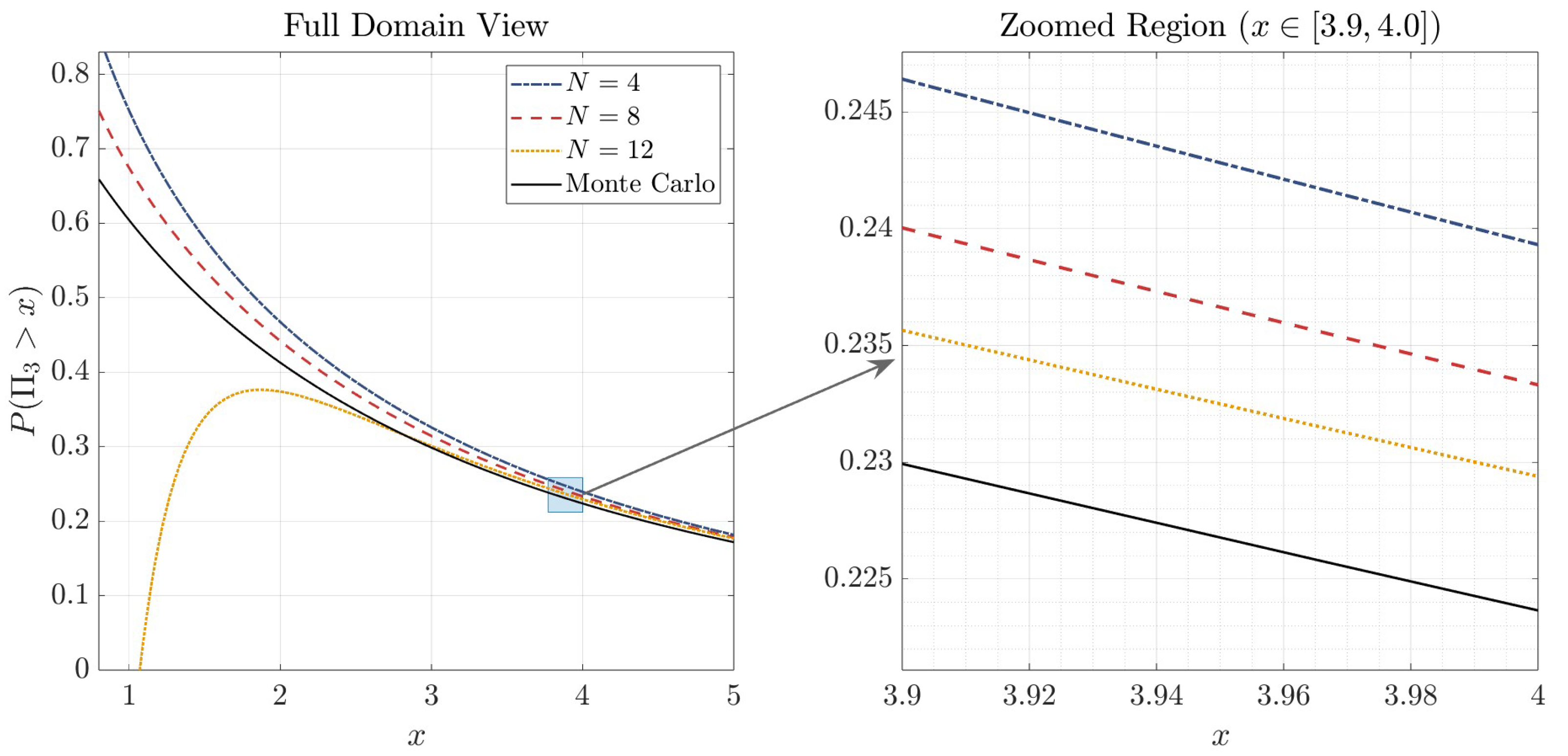
Consider the product ${\Pi }_3={\xi }_1{\xi }_2{\xi }_3$ of three independent random variables ${\xi }_1$, ${\xi }_2$, ${\xi }_3$, each following the Weibull distribution with parameters $\alpha =1.5$ and $\beta =0.5$. According to Theorem 1, for $N=12$, we obtain

$$\begin{array}{cc}\hfill {\overline{F}}_{{\Pi }_3}\left(x\right)& ={\displaystyle \frac{\pi }{\sqrt{3}}}{\mathrm{e}}^{-1.5x^{1/2}}{x}^{1/2}(1+2x^{-1/2}{\mathcal{D}}_{2,3}+4x^{-1}{\mathcal{D}}_{4,3}+8x^{-3/2}{\mathcal{D}}_{6,3}\hfill \\ \hfill & +16x^{-2}{\mathcal{D}}_{8,3}+32x^{-5/2}{\mathcal{D}}_{10,3}+64x^{-3}{\mathcal{D}}_{12,3}+O\left(x^{-13/4}\right)),\hfill \end{array}$$

where

$$\begin{array}{cc}\hfill {\mathcal{D}}_{2,3}& ={\displaystyle \frac{2}{9}},{\mathcal{D}}_{4,3}={\displaystyle \frac{533}{5184}},{\mathcal{D}}_{6,3}=-{\displaystyle \frac{95705}{2239488}},\hfill \\ \hfill {\mathcal{D}}_{8,3}& ={\displaystyle \frac{1532695}{161243136}},{\mathcal{D}}_{10,3}={\displaystyle \frac{233444225}{11609505792}},{\mathcal{D}}_{12,3}=-{\displaystyle \frac{419317617635}{10030613004288}}.\hfill \end{array}$$

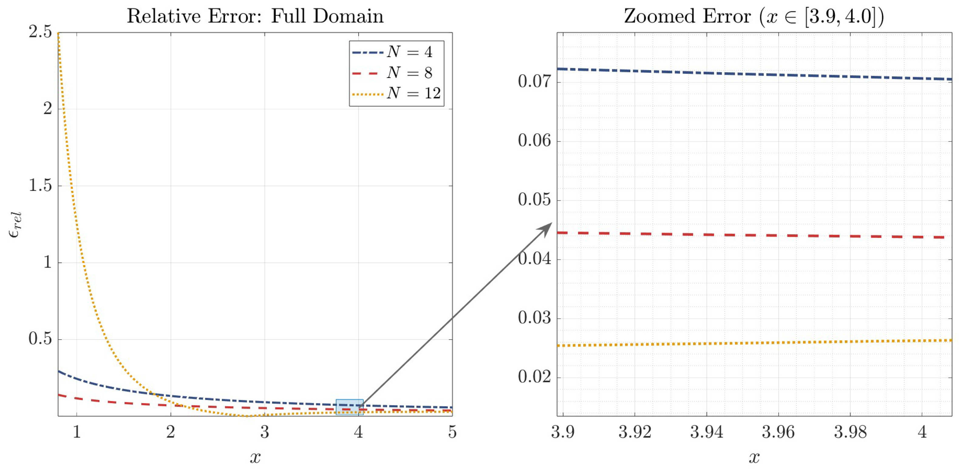
In Figure 1, we present the graphs of the tail function ${\overline{F}}_{{\Pi }_3}\left(x\right)$ obtained by the Monte Carlo simulation and the graphs of the asymptotic approximations of this tail function with two $(N=4)$, four $(N=8)$, and six $(N=12)$ remainder terms. As predicted, the results indicate that approximations with six remainder terms provide the most accurate tail fit, especially for large values of x. However, this higher-order expansion exhibits instability for small x (around $x<2.5$). The relative errors for asymptotic values of the function ${\overline{F}}_{{\Pi }_3}\left(x\right)$ are presented in Figure 2.

Example 2. 

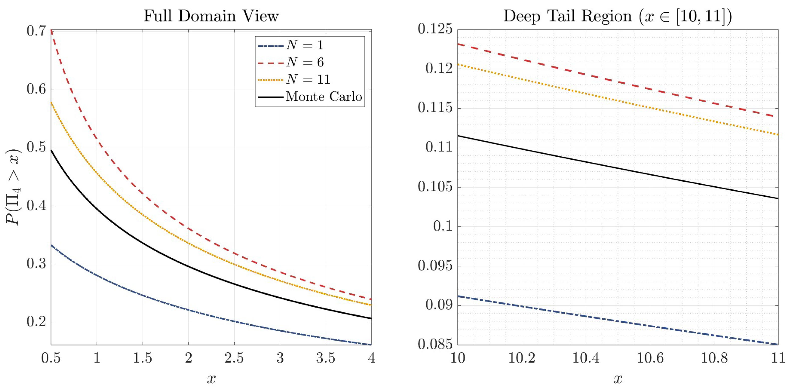
Consider ${\Pi }_4={\xi }_1{\xi }_2{\xi }_3{\xi }_4$ corresponding to four i.i.d. Weibull random variables ${\xi }_i$ with parameters $\alpha =0.9$ and $\beta =0.7$. According to Theorem 1, for $N=11$, we get

$$\begin{array}{cc}\hfill {\overline{F}}_{{\Pi }_4}\left(x\right)& ={\displaystyle \frac{{\left(1.4\pi \right)}^{3/2}}{2}}{\mathrm{e}}^{-2.8x^{9/40}}{x}^{27/80}(1+{\displaystyle \frac{10}{7}}{x}^{-9/40}{\mathcal{D}}_{2,4}+{\displaystyle \frac{100}{49}}{x}^{-9/20}{\mathcal{D}}_{4,4}\hfill \\ & +{\displaystyle \frac{1000}{343}}{x}^{-27/40}{\mathcal{D}}_{6,4}+{\displaystyle \frac{10000}{2401}}{x}^{-9/10}{\mathcal{D}}_{8,4}+{\displaystyle \frac{100000}{16807}}{x}^{-9/8}{\mathcal{D}}_{10,4}+O\left(x^{-27/20}\right)),\hfill \end{array}$$

where

$${\mathcal{D}}_{2,4}={\displaystyle \frac{7}{32}},{\mathcal{D}}_{4,4}={\displaystyle \frac{10147}{55296}},{\mathcal{D}}_{6,4}={\displaystyle \frac{272813}{5308416}},{\mathcal{D}}_{8,4}={\displaystyle \frac{-366867965}{6115295232}},{\mathcal{D}}_{10,4}={\displaystyle \frac{36705411835}{5283615080448}}.$$

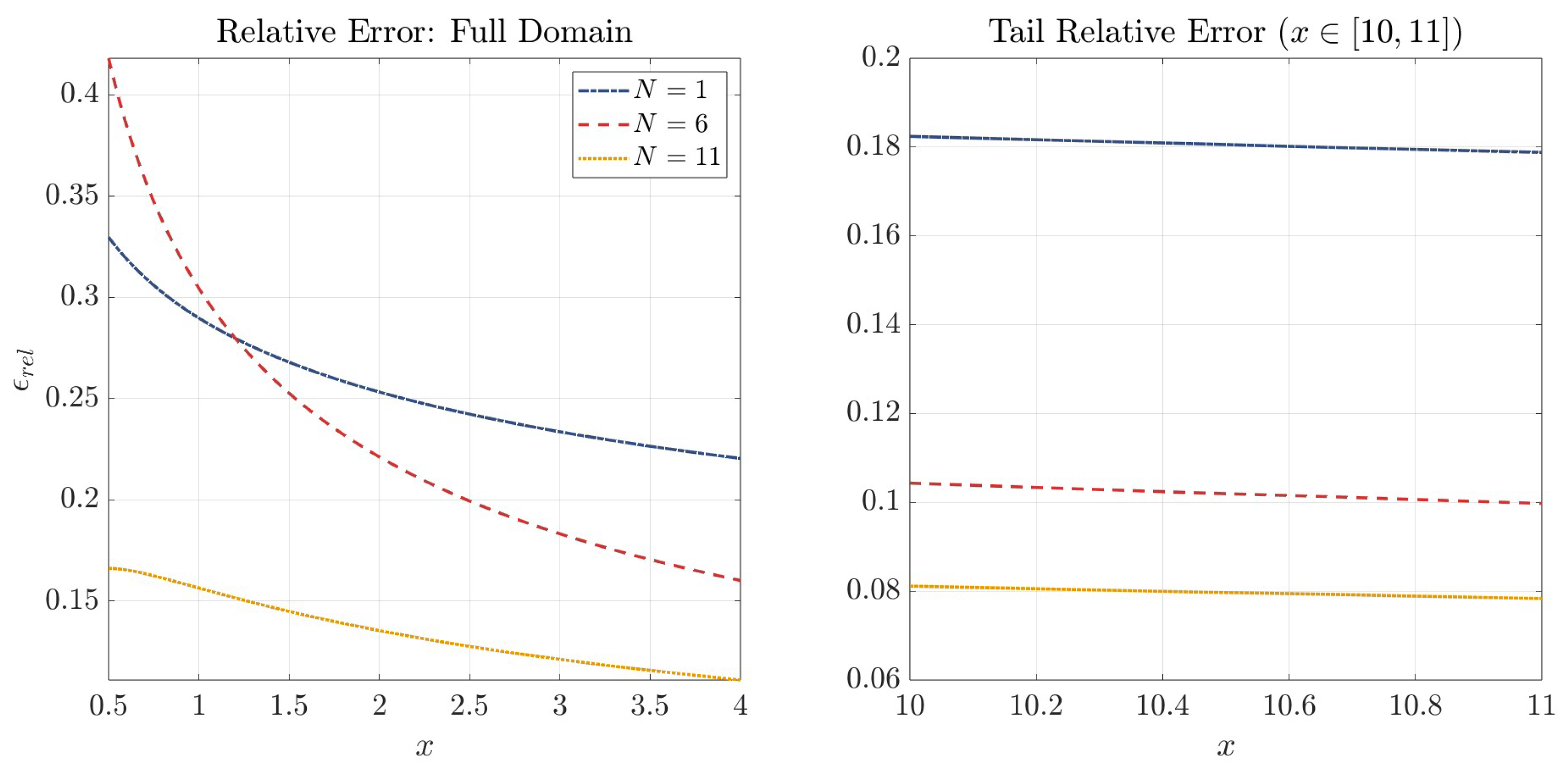
In Figure 3, we present the graphs of the tail function ${\overline{F}}_{{\Pi }_4}\left(x\right)$ obtained by the Monte Carlo simulations and the graphs of the asymptotic approximations of this tail function without $(N=1)$, three $(N=6)$, and five $(N=11)$ remainder terms. It is easy to see that, as in the first example, the values of the asymptotic approximations of the function ${\overline{F}}_{{\Pi }_4}\left(x\right)$ with a larger number of remainder terms are closer to the “true” values of this function. Note that, unlike the first example, the values of the asymptotic approximations are close to the “true” values of the function ${\overline{F}}_{{\Pi }_4}\left(x\right)$ for relatively small x, but for relatively large x the asymptotic approximations in Example 2 are worse than in Example 1. Apparently, this is influenced by the heaviness of the multiplied random variables. This effect can be easily observed in the graphs of Figure 4.

8. Conclusions

In this paper, we examine the asymptotic behavior of the product of identically distributed Weibull random variables. We derived an explicit asymptotic expansion for the tail of the product distribution and provided a recursive procedure for computing the coefficients, which was numerically validated through Monte Carlo simulations. The study illustrates how classical asymptotic techniques, such as the Laplace method, can be adapted to solve problems involving products of random variables. Our results offer insight into the influence of the Weibull shape parameter on the decay rate of the tail distribution. Moreover, the proposed framework is flexible and can be extended to other families of light- and heavy-tailed distributions. These findings have potential applications in reliability theory, risk analysis, and related areas where products of random variables naturally arise. Although we specifically considered i.i.d. Weibull r.v.s, the approach is readily extensible to generalized Weibull-type distributions.

References

1. Chen, Y.; Karagiannidis, G.K.; Lu, H.; Cao, N. Novel approximations to the statistics of products of independent random variables and their applications in wireless communications. IEEE Trans. Veh. Technol. 2012, 61, 443–454. [Google Scholar] [CrossRef]
2. Abo Rahama, Y.; Ismail, M.H.; Hassan, M.S. On the distribution of the product and ratio of products of EGK variates with applications. Telecommun. Syst. 2018, 68, 231–238. [Google Scholar] [CrossRef]
3. Du, H.; Zhang, J.; Peppas, K.P.; Zhao, H.; Ai, B.; Zhang, X. On the distribution of the ratio of products of Fisher–Snedecor F random variables and its applications. IEEE Trans. Veh. Technol. 2020, 69, 1855–1866. [Google Scholar] [CrossRef]
4. Shekhar, S.; Kalyani, S. Product and ratio of two α-κ-μ shadowed random variables and its application to wireless communication. IEEE Access 2025, 13, 190388–190402. [Google Scholar] [CrossRef]
5. Wille, E.C.G. Efficient approximation to Rician and Hoyt product distributions with applications to wireless communication channels. IEEE Wirel. Commun. Lett. 2025, 14, 3254–3258. [Google Scholar] [CrossRef]
6. Chen, Y.; Ng, K.W.; Yuen, K.C. The maximum of randomly weighted sums with long tails in insurance and finance. Stoc. Anal. Appl. 2011, 29, 1033–1044. [Google Scholar] [CrossRef][Green Version]
7. Asimit, A.V.; Hashorva, E.; Kortschak, D. Aggregation of randomly weighted large risks. IMA J. Manag. Math. 2017, 28, 403–419. [Google Scholar] [CrossRef][Green Version]
8. Jaunė, E.; Ragulina, O.; Šiaulys, J. Expectation of the truncated randomly weighted sums with dominatedly varying summands. Lith. Math. J. 2018, 58, 421–440. [Google Scholar] [CrossRef]
9. Gong, Y.; Yang, Y.; Liu, J. On the Kesten-type inequality for randomly weighted sums with applications to an operational risk model. Filomat 2021, 35, 1879–1888. [Google Scholar] [CrossRef]
10. Konstantinides, D.G.; Passalidis, C.D. Background risk model in presence of heavy tails under dependence. Nonlinear Anal. Model. Control 2025, 30, 982–1010. [Google Scholar] [CrossRef]
11. Rekha, A.; Sunder, T.S. Survival function of a component under random strength attenuation. Microelectron. Reliab. 1997, 37, 677–681. [Google Scholar] [CrossRef]
12. Nadarajah, S.; Kotz, S. On the product and ratio of gamma and beta random variables. Allg. Stat. Arch. 2005, 89, 435–449. [Google Scholar] [CrossRef]
13. Coelho, C.A.; Alberto, R.P. On the distribution of the product of independent beta random variables—Applications. In Advances in Statistics—Theory and Applications. Emerging Topics in Statistics and Biostatistics; Ghosh, I., Balakrishnan, N., Ng, H.K.T., Eds.; Springer: Cham, Switzerland, 2021. [Google Scholar]
14. De Carlo, F. Reliability and maintainability in operations management. In Operations Management; Schiraldi, M.M., Ed.; IntechOpen: London, UK, 2013; pp. 81–111. [Google Scholar] [CrossRef]
15. Springer, M.D. The Algebra of Random Variables; John Wiley and Sons: Hoboken, NJ, USA, 1979. [Google Scholar]
16. Galambos, J.; Simonelli, I. Products of Random Variables: Applications to Problems of Physics and to Arithmetical Functions; Taylor and Francis: Boca Raton, FL, USA, 2004. [Google Scholar]
17. Lomnicki, Z.A. On the distribution of products of random variables. J. R. Stat. Soc. Ser. B Stat. Methodol. 1967, 29, 513–524. [Google Scholar] [CrossRef]
18. Lawless, J.F. Statistical Models and Methods for Lifetime Data; Wiley: New York, NY, USA, 1982. [Google Scholar]
19. Abernethy, R.B. The New Weibull Handbook. Reliability and Statistical Analysis for Predicting Life, Safety, Survivability, Risk, Cost, and Warranty Claims, 5th ed.; Robert B. Abernethy: North Palm Beach, FL, USA, 2004. [Google Scholar]
20. Hogg, R.V.; Klugman, S.A. Loss Distributions; Wiley: New York, NY, USA, 1984. [Google Scholar]
21. Li, J.; Liu, J. Claims modeling with three-component composite models. Risks 2023, 11, 196. [Google Scholar] [CrossRef]
22. Mittnik, S.; Rachev, S.T. Stable distributions for asset returns. Appl. Math. Lett. 1989, 2, 301–304. [Google Scholar] [CrossRef]
23. Mittnik, S.; Rachev, S.T. Modelling asset returns with alternative stable distributions. Econom. Rev. 1993, 12, 261–330. [Google Scholar] [CrossRef]
24. Bardley, R.F.; McDonald, J.B.; Mantrala, A. Something new, something old: Parametric models for the size distribution of income. J. Income Distrib. 1996, 6, 91–103. [Google Scholar] [CrossRef]
25. Stoyan, D.; Zhang, Z.X. A stochastic model leading to various particle mass distributions including the RRSB distribution. Granul. Matter 2023, 25, 67. [Google Scholar] [CrossRef]
26. Zhang, Z.T.; Xu, Y.X.; Liao, J.B.; Liu, S.K.; Liu, Z.; Gao, W.H.; Yi, L.W. Study on the particle strength and crushing patterns of coal gangue coarse-grained subgrade fillers. Sustainability 2024, 16, 5155. [Google Scholar] [CrossRef]
27. Medhi, J. Stochastic Models in Queueing Theory, 2nd ed.; Academic Press: Cambridge, MA, USA, 2002. [Google Scholar]
28. Akbash, K.; Matsak, I.; Zakusylo, O. Some limit theorems for extreme values of Lindley-type processes. Lith. Math. J. 2025, 65, 1–13. [Google Scholar] [CrossRef]
29. Johnson, N.L.; Kotz, S.; Balakrishnan, N. Continuous Univariate Distributions, 2nd ed.; Wiley: New York, NY, USA, 1994. [Google Scholar]
30. Kotz, S.; Nadarajah, S. Extreme Value Distributions. Theory and Applications; Imperial College Press: London, UK, 2000. [Google Scholar]
31. Ianculescu, D.; Anghel, C.G. Innovative explicit relations for Weibull distribution parameters based on K-moments. Mathematics 2025, 13, 3473. [Google Scholar] [CrossRef]
32. Tang, Q. From light tails to heavy tails through multiplier. Extremes 2008, 11, 379–391. [Google Scholar] [CrossRef]
33. Arendarczyk, M.; Dȩbicki, K. Asymptotics of supremum distribution of a Gaussian process over a Weibullian time. Bernoulli 2011, 17, 194–210. [Google Scholar] [CrossRef]
34. Dȩbicki, K.; Farkas, J.; Hashorva, E. Extremes of randomly scaled Gumbel risks. J. Math. Anal. Appl. 2018, 458, 30–42. [Google Scholar] [CrossRef]
35. Leipus, R.; Šiaulys, J.; Dirma, M.; Zovė, R. On the distribution-tail behaviour of the product of normal random variables. J. Inequal. Appl. 2023, 2023, 32. [Google Scholar] [CrossRef]
36. Kamarauskas, R.; Šiaulys, J. On the distribution-tail of the product of gamma random variables. Nonlinear Anal. Model. Control 2024, 29, 1180–1199. [Google Scholar] [CrossRef]
37. Bose, A.; Hazra, R.S.; Saha, K. Product of exponentials and spectral radius of random k-circulants. Ann. L’Institute Henri Poincaré 2012, 48, 424–443. [Google Scholar] [CrossRef]
38. Hashorva, E.; Weng, Z. Tail asymptotic of Weibull-type risks. Statistics 2014, 48, 1155–1165. [Google Scholar] [CrossRef]
39. Watson, G.N. The harmonic functions associated with the parabolic cylinder. Proc. Lond. Math. Soc. 1918, 2, 116–148. [Google Scholar] [CrossRef]
40. Wong, R. Asymptotic Approximations of Integrals; Academic Press: Berlin/Heidelberg, Germany, 1989. [Google Scholar]
41. Olver, F.W.J. Asymptotics and Special Functions; A K Peters/CRC Press: Boca Raton, FL, USA, 1997. [Google Scholar]
42. Miller, P.D. Applied Asymptotic Analysis; American Mathematical Society: Providence, RI, USA, 2006. [Google Scholar]
43. Erdélyi, A. Asymptotic Expansions; Dover Publications: New York, NY, USA, 1956. [Google Scholar]
44. De Bruijn, N.G. Asymptotic Methods in Analysis, 2nd ed.; North-Holland: Amsterdam, The Netherlands, 1961. [Google Scholar]
45. Copson, E.T. Asymptotic Expansions; Cambridge University Press: Cambridge, UK, 1965. [Google Scholar]
46. Bender, C.M.; Orszag, S.A. Advanced Mathematical Methods for Scientists and Engineers: Asymptotic Methods and Perturbation Theory; McGraw–Hill: New York, NY, USA, 1978. [Google Scholar]
47. Butler, R.W. Saddlepoint Approximations with Applications; Cambridge University Press: Cambridge, UK, 2007. [Google Scholar]
48. Wojdylo, J. On the coefficients that arise from Laplace’s method. J. Comput. Appl. Math. 2006, 196, 241–266. [Google Scholar] [CrossRef]
49. Wojdylo, J. Computing the Coefficients in Laplace’s Method. SIAM Rev. 2006, 48, 76–96. [Google Scholar] [CrossRef]
Figure 1. Tail probability of product of three i.i.d. Weibull r.v.s with α = 1.5 , β = 0.5 .
Mathematics 14 00736 g001
Figure 2. Relative errors for asymptotic values of function F ¯ Π 3 ( x ) .
Mathematics 14 00736 g002
Figure 3. Tail probability of product of four i.i.d. Weibull r.v.s with parameters α = 0.9 , β = 0.7 .
Mathematics 14 00736 g003
Figure 4. Relative errors for asymptotic values of function F ¯ Π 4 ( x ) .
Mathematics 14 00736 g004
Disclaimer/Publisher’s Note: The statements, opinions and data contained in all publications are solely those of the individual author(s) and contributor(s) and not of MDPI and/or the editor(s). MDPI and/or the editor(s) disclaim responsibility for any injury to people or property resulting from any ideas, methods, instructions or products referred to in the content.