Article

Synchronization of Delay Switched Fractional Cohen–Grossberg Neural Network Models

by
Donal O’Regan
1 and
Snezhana Hristova
2,*
1
School of Mathematical and Statistical Sciences, University of Galway, H91 TK33 Galway, Ireland
2
Faculty of Mathematics and Informatics, University of Plovdiv, Tzar Asen 24, 4000 Plovdiv, Bulgaria
*
Author to whom correspondence should be addressed.
Mathematics 2026, 14(4), 726; https://doi.org/10.3390/math14040726
Submission received: 20 January 2026 / Revised: 9 February 2026 / Accepted: 17 February 2026 / Published: 19 February 2026

Abstract

The Cohen–Grossberg neural network is studied in the case when the dynamics of the neurons are modeled by generalized Caputo fractional derivatives with respect to another function (GCFDF). We consider a time-dependent delay and a switching rule in the model, which specifies when to switch the system at the initially given times. The switching rule is a piecewise constant function, and its points of discontinuity are the lower limits of the applied GCFDF on the corresponding intervals. We develop theoretical tools for GCFDF, starting with an important inequality for estimating that derivative on quadratic functions. We define the global Mittag–Leffler synchronization and obtain sufficient conditions based on the Lyapunov method, using a Razumikhin condition and quadratic functions.

1. Introduction

Fractional derivatives are widely studied and applied, and there are various types of fractional derivatives with different properties. The main common property of fractional derivatives is connected with the memory, which differs from integer order derivatives. These types of derivatives are not only studied theoretically but are also applied in modeling; for example, they are used in the modeling of neural networks. One of the hot research topics in complex systems is synchronization (see, for example, [1,2]). When fractional derivatives are applied, the most appropriate type is Mittag–Leffler synchronization (MLS). We mention MLS [3] for impulsive fractional-order neural networks with delays, Ref. [4] for delayed fractional-order bidirectional associative memory neural networks, Ref. [5] for variable-order fractional reaction-diffusion networks, Ref. [6] for fractional neural networks with time-varying delays and reaction-diffusion terms, Ref. [7] for MLS of fractional-order complex-valued memristive neural networks with time delay, Ref. [8] for MLS of fractional neural networks with distributed delays, Ref. [9] for fractional BAM neural networks with linear feedback controllers, Ref. [10] for delayed fractional memristive neural networks.
One of the most useful models is the Cohen–Grossberg model of neural networks (CGM), which is studied in various forms when modeling the dynamics of neurons. The main difference between the Cohen–Grossberg neural network model (CGM) [11] and other neural network models lies in the system of equations that describes neuronal dynamics. In CGN, the state is multiplied by a gain function, allowing modeling of biological neural saturation. Also, CGM is a generalization of some known models in the literature, such as the Hopfield neural network [12]. Recently, many different generalizations of CGM have been presented, and their properties have been studied. For example, in [13] MLS of fractional memristive CGM with state feedback and impulsive control is studied, and in [14] a coupled delayed fractional reaction-diffusion (CGM) is investigated.
In this paper, we study the synchronization of a special model of Cohen–Grossberg neural network with a variable delay (CGNND). First, for modeling the dynamics of the neurons, we use a generalization of the fractional derivative, the so-called Caputo fractional derivative with respect to another function (studied theoretically in [15] and applied to CGNND in [16]) and its generalization introduced in [17]. Second, we consider the case where a switching rule changes at certain times in the activation functions and in some of the applied coefficients (see, for example, [18]). Note that synchronization of some types of switched fractional models is studied in [19,20]. In this paper, we consider a piecewise-constant switching rule with an initially specified set of CGNND and switching times. We present an algorithm for constructing a solution to the switched CGNND, define Mittag–Leffler synchronization for the model under study, and obtain sufficient conditions. The obtained results generalize several known results in the literature.
The main contributions of this paper could be summarized as follows:
-
A generalization of the classical Cohen–Grossberg neural network model is considered in the case when
-
there is a delay;
-
the dynamic of the neurons is described by a Caputo fractional derivative with respect to another function;
-
there is a switching rule which allows us to describe adequately the change of the dynamics of neurons at some initially given points;
-
Switching times in the model could be finite or infinite;
-
Short memories are considered, i.e., the lower limits of the applied fractional derivative are changing at any switching time;
-
Mittag–Leffler synchronization of the model is studied, and some sufficient conditions are obtained.
-
the basis of the study are quadratic Lyapunov functions and the Razumikhin method.

2. Preliminary Notes on Generalized Caputo Fractional Derivatives with Respect to Another Function

We will present results from the literature on the main definitions and on applied fractional derivatives.
Let a , T : 0 a < T . We will use the following sets of functions:
C 1 ( ( a , T ] , R n ) = { u C ( ( a , T ] , R n ) : u exists   and   it   is   continuous   on ( a , T ] } ,
and
P ( a , T ) = { ψ C 1 ( [ a , T ] , [ 0 , ) ) : ψ ( t ) > 0 , t ( a , T ] } .
Definition 1
([17])). Let q > 0 , ρ > 0 , and the function ψ P ( a , T ) . The generalized fractional integral with respect to another function (FIF) of the function υ : [ a , T ] R is defined by (where the integral exists)
I a q , ψ ρ υ ( t ) = ρ 1 q Γ ( q ) a t ψ ( s ) ρ 1 ψ ( s ) υ ( s ) ψ ( t ) ρ ψ ( s ) ρ 1 q d s , t ( a , T ] .
Definition 2
([17]). Let q ( 0 , 1 ) , ρ > 0 and the function ψ P ( a , T ) . The generalized Caputo fractional derivative with respect to another function (GCFDF) of the function υ : [ a , T ] R is defined by (where the integral exists)
D a q , ψ ρ C υ ( t ) = ρ q Γ ( 1 q ) a t υ ( s ) ( ψ ( t ) ) ρ ( ψ ( s ) ) ρ q d s , t ( a , T ] .
In the case of vector functions the integral FIF and the derivative GCFDF are defined component-wise.
In connection with Definition 2 we will introduce the following set of functions:
C q ( ( a , T ] , ψ , ρ ) = { u C ( ( a , T ] , R n ) : u exists   almost   everywhere   in ( a , T ] and   there   exists   GCFDF   D a q , ψ ρ C u ( t ) for t ( a , T ] } .
We will use the following results for GCFDF.
Lemma 1.
Let ρ > 0 , q ( 0 , 1 ) , ψ P ( a , T ) . Then
D a q , ψ ρ C ψ ( t ) ρ ( ψ ( a ) ) ρ ρ β 1 = Γ ( β ) Γ ( β q ) ψ ( t ) ρ ( ψ ( a ) ρ ρ β q 1 , t ( a , T ] ,
where β > 1 .
Proof. 
Define the function f ( t ) = ψ ( t ) ρ ( ψ ( a ) ) ρ ρ β 1 for t ( a , T ] . Then
f ( t ) = ( β 1 ) ψ ( t ) ρ 1 ψ ( t ) ψ ( t ) ρ ( ψ ( a ) ) ρ ρ β 1 , t ( a , T ] ,
and
D a q , ψ ρ C f ( t ) = ρ q Γ ( 1 q ) a t ( β 1 ) ψ ( s ) ρ 1 ψ ( s ) ψ ( s ) ρ ( ψ ( a ) ) ρ ρ β 1 ( ψ ( t ) ) ρ ( ψ ( s ) ) ρ q d s = ( β 1 ) ρ q + β 1 Γ ( 1 q ) a t ψ ( s ) ρ ( ψ ( a ) ) ρ β 2 ( ψ ( t ) ) ρ ( ψ ( s ) ) ρ q d ψ ( s ) ρ = ( β 1 ) ρ β 1 q Γ ( 1 q ) a t ψ ( s ) ρ ( ψ ( a ) ) ρ β 2 ( ψ ( t ) ) ρ ( ψ ( s ) ) ρ q d ψ ( s ) ρ = ( β 1 ) ρ β 1 q Γ ( 1 q ) ψ ( t ) ρ ( ψ ( a ) ) ρ β 2 q + 1 a t 1 ( ψ ( s ) ρ ( ψ ( a ) ) ρ ) ψ ( t ) ρ ( ψ ( a ) ) ρ q × ψ ( s ) ρ ( ψ ( a ) ) ρ ψ ( t ) ρ ( ψ ( a ) ) ρ β 2 d ( ψ ( s ) ρ ( ψ ( a ) ) ρ ) ψ ( t ) ρ ( ψ ( a ) ) ρ = ( β 1 ) ρ β 1 q Γ ( 1 q ) ψ ( t ) ρ ( ψ ( a ) ) ρ β 1 q 0 1 1 u q u β 2 d u = ( β 1 ) ρ β 1 q Γ ( 1 q ) ψ ( t ) ρ ( ψ ( a ) ) ρ β 2 q B ( 1 q , β 1 ) = ( β 1 ) ρ β 1 q Γ ( 1 q ) ψ ( t ) ρ ( ψ ( a ) ) ρ β 2 q Γ ( 1 q ) Γ ( β 1 q ) Γ ( 1 q + β 1 ) = ( β 1 ) ρ β 1 q Γ ( β 1 ) Γ ( β q ) ψ ( t ) ρ ( ψ ( a ) ) ρ β 1 q = Γ ( β ) Γ ( β q ) ψ ( t ) ρ ( ψ ( a ) ) ρ ρ β 1 q
where u = ψ ( s ) ρ ( ψ ( a ) ) ρ ψ ( t ) ρ ( ψ ( a ) ) ρ and B ( x , y ) = 0 1 t x 1 ( 1 t ) y 1 d t = Γ ( x ) Γ ( y ) Γ ( x + y ) . □
From Lemma 1, we obtain the following result:
Corollary 1.
Let ρ > 0 , q ( 0 , 1 ) , ψ P ( a , T ) and λ R be a constant. Then
D a q , ψ ρ C E q λ ψ ( t ) ρ ( ψ ( a ) ) ρ ρ q = λ E q λ ψ ( t ) ρ ( ψ ( a ) ) ρ ρ q , t ( a , T ] ,
where E q is the Mittag–Leffler function with one parameter.
Proof. 
We note that
E q λ ψ ( t ) ρ ( ψ ( a ) ) ρ ρ q = k = 0 1 Γ ( q k + 1 ) λ k ψ ( t ) ρ ( ψ ( a ) ) ρ ρ k q .
Take the GCFDF on both sides of (3), use Lemma 1 for β = q k + 1 , and obtain
D a q , ψ ρ C E q λ ψ ( t ) ρ ( ψ ( a ) ) ρ ρ q = k = 0 λ k Γ ( q k + 1 ) D a q , ψ ρ C ψ ( t ) ρ ( ψ ( a ) ) ρ ρ q k = k = 1 λ k Γ ( q k + 1 ) Γ ( q k + 1 ) Γ ( q k + 1 q ) ψ ( t ) ρ ( ψ ( a ) ρ ρ q k q = k = 0 λ k + 1 Γ ( q k + 1 ) ψ ( t ) ρ ( ψ ( a ) ρ ρ q k .
From Corollary 1, we have the following result:
Lemma 2.
Let ρ > 0 , q ( 0 , 1 ) , ψ P ( a , T ) and λ R be a constant. The solution of the scalar linear fractional initial value problem with GCFDF
D a q , ψ ρ C u ( t ) = λ u ( t ) , f o r t ( a , T ] , a n d u ( a ) = u 0 ,
is the function
u ( t ) = u 0 E q λ ψ ( t ) ρ ( ψ ( a ) ) ρ ρ q , t [ a , T ] .
Lemma 3
([18]). Let ρ > 0 , q ( 0 , 1 ) , ψ P ( a , T ) , υ : [ a , T ] R , a < T and there exists a point ξ ( a , T ] such that υ ( ξ ) = 0 , and υ ( t ) > ( < ) 0 , for t [ a , ξ ) and the GCFDF D a q , ψ ρ C υ ( t ) | t = ξ exists. Then if lim s ξ υ ( s ) ( ( ψ ( ξ ) ) ρ ( ψ ( s ) ) ρ ) q = 0 we have D a q , ψ ρ C υ ( t ) | t = ξ ( ) 0 .
Remark 1
([18]). In Lemma 3 if u C 1 ( [ a , T ] , R ) then L’Hopital’s rule guarantees that
lim s ξ u ( s ) ( ψ ( ξ ) ) ρ ( ψ ( s ) ) ρ q = lim s ξ u ( s ) ( ψ ( ξ ) ) ρ ( ψ ( s ) ) ρ 1 q q ρ ( ψ ( s ) ) ρ 1 ψ ( s ) = 0 .
Note that from ξ > a and ψ ( s ) > 0 , s [ a , ξ ] it follows that ψ ( ξ ) > 0 .
We could also put other conditions (other than u C 1 ( [ a , T ] , R ) ), for example, instead one could assume lim s ξ u ( s ) exists and is a real number) to guarantee that this limit is zero.
We will prove some new results for scalar functions and their GCFDF, which will be applied in the proofs of the main results in the next sections. Also, they are of value any time GCFDF is studied.
Lemma 4.
Let u C q ( [ a , T ] , R , ψ , ρ ) be such that u 2 C q ( [ a , T ] , R , ψ , ρ ) . Then
D a q , ψ ρ C u 2 ( t ) 2 u ( t ) D a q , ψ ρ C u ( t ) f o r a l l t ( a , T ] ,
where a , T R : 0 a < T .
Proof. 
For any fixed τ ( a , T ] we define the function v t : [ a , T ] [ 0 , ) by
v t ( s ) = u ( τ ) u ( s ) 2 , s [ a , T ] .
Note that v t C q ( [ a , T ] , [ 0 , ) , ψ , ρ ) , v t ( s ) > 0 , s [ a , τ ) and v t ( τ ) = 0 , so v satisfies the assumptions of Lemma 3, and, therefore, D a q , ψ ρ C v t ( τ ) 0 .
Thus,
D a q , ψ ρ C u 2 ( τ ) 2 u ( τ ) D a q , ψ ρ C u ( τ ) = ρ q Γ ( 1 q ) a τ d d σ u 2 ( σ ) 2 u ( τ ) u ( σ ) ( ψ ( τ ) ) ρ ( ψ ( σ ) ) ρ q d σ = ρ q Γ ( 1 q ) a τ 2 u ( σ ) u ( τ ) u ( σ ) ( ψ ( τ ) ) ρ ( ψ ( σ ) ) ρ q d σ = ρ q Γ ( 1 q ) a τ v ( σ ) ( ψ ( τ ) ) ρ ( ψ ( σ ) ) ρ q d σ = D a q , ψ ρ C v ( τ ) 0 .
In the case of non-negative scalar functions we have the following result:
Lemma 5.
Assume the following:
1. 
The function u C q ( [ a , T ] , [ 0 , ) , ψ , ρ ) C ( [ a μ , a ] , [ 0 , ) ) with μ > 0 .
2. 
The function Λ C ( [ μ , 0 ] , ( 0 , 1 ] ) and for any t ( a , T ] such that
max θ [ μ , 0 ] u ( t + θ ) Λ ( θ ) u ( t )
the inequality
D a q , ψ ρ C u ( t ) λ u ( t )
holds with λ > 0 .
  • Then
u ( s ) u ( a ) E q λ ψ ( s ) ρ ( ψ ( a ) ) ρ ρ q f o r a l l s [ a , T ] .
Proof. 
Let ε > 0 be an arbitrary number. We define
η ( s , ε ) = u ( s ) u ( a ) E q λ ψ ( s ) ρ ( ψ ( a ) ) ρ ρ q ε , f o r s [ a , T ] .
According to Condition 1 the function η C q ( [ a , T ] , R , ψ , ρ ) and
D a q , ψ ρ C η ( t , ε ) = D a q , ψ ρ C u ( t ) + λ u ( a ) E q λ ψ ( t ) ρ ( ψ ( a ) ) ρ ρ q , t ( a , T ] .
Since E q λ ψ ( a ) ρ ( ψ ( a ) ) ρ ρ q = 1 , we get η ( a , ε ) = u ( a ) u ( a ) ε < 0 .
We claim
η ( s , ε ) < 0 for all s [ a , T ] .
Assume that (12) is not true on [ a , T ] , i.e., there exists a point ν ( a , T ] such that
η ( s , ε ) < 0 for all s [ a , ν ) and η ( ν , ε ) = 0 .
Note that the function η satisfies the assumptions of Lemma 3 with ξ = ν and u ( . ) = η ( . , ε ) . According to Lemma 3, Remark 1 and the choice of the point ν , we have
D a q , ψ ρ C η ( t , ε ) | t = ν 0 .
We need to consider the following two cases:
Case 1.
Let ν ( μ , T ] . Then for all θ [ μ , 0 ) we have ν + θ > 0 and from 0 < Λ ( θ ) 1 and (13) we have η ( ν + θ , ε ) < 0 and
u ( ν + θ ) Λ ( θ ) < ( u ( a ) E q λ ψ ( ν ) ρ ( ψ ( a ) ) ρ ρ q + ε ) Λ ( θ ) = ( u ( a ) E q λ ψ ( ν ) ρ ( ψ ( a ) ) ρ ρ q + ε ) Λ ( θ ) + η ( ν , ε ) = u ( ν ) u ( a ) E q λ ψ ( ν ) ρ ( ψ ( a ) ) ρ ρ q + ε 1 Λ ( θ ) u ( ν ) .
Inequality (15) proves the Razumikhin-type condition (8) is satisfied for t = ν .
Case 2.
Let ν ( a , μ ] . Then for any θ [ μ , 0 ] there are two possibilities: ν + θ [ a μ , a ] or ν + θ ( a , μ ] .
If ν + θ ( a , μ ] similar to Case 1 and (15), we have
u ( ν + θ ) Λ ( θ ) u ( ν ) .
If ν + θ [ a μ , a ] then applying Λ ( θ ) > 0 , we get
u ( ν + θ ) Λ ( θ ) u ( ν + θ ) u ( a ) < ( u ( a ) + ε ) = η ( ν , ε ) + ( u ( a ) + ε ) = u ( ν ) .
Therefore, the inequality (8) (the Razumikhin-type condition) holds for t = ν in this case.
Therefore, D a q , ψ ρ C u ( ν ) λ u ( ν ) = 0 . Then, applying (11) and Corollary 1, we get
D a q , ψ ρ C η 2 ( ν , ε ) = D a q , ψ ρ C u ( ν ) λ u ( a ) E q λ ψ ( ν ) ρ ( ψ ( a ) ) ρ ρ q λ E q λ ψ ( ν ) ρ ( ψ ( a ) ) ρ ρ q λ u ( a ) E q λ ψ ( ν ) ρ ( ψ ( a ) ) ρ ρ q < 0 .
Now (17) contradicts (14), proving (12). Since (12) is satisfied for an arbitrary ε after taking the limit as ε 0 , we get
η ( s , 0 ) = u ( s ) u ( a ) E q λ ψ ( s ) ρ ( ψ ( a ) ) ρ ρ q 0
which implies (10). □
Remark 2.
Condition 2 of Lemma 5 is a Razumikhin condition. Note, inequality (9) is not satisfied for all points t ( a , T ] but only for those satisfying the inequality (8). This is very important in the application of Lyapunov functions to study stability properties of any system with delays.
Denote R + n = [ 0 , ) × [ 0 , ) × [ 0 , ) .
Corollary 2.
Assume the following:
1. 
The function x C q ( [ a , T ] , R n , ψ , ρ ) C ( [ a μ , a ] , R n ) and x 2 C q ( [ a , T ] , R + n , ψ , ρ ) C ( [ a μ , a ] , R + n ) where x = ( x 1 , x 2 , , x n ) , x 2 = ( x 1 2 , x 2 2 , , x n 2 ) , μ > 0 .
2. 
The function Λ C ( [ μ , 0 ] , ( 0 , 1 ] ) is such that for any t ( a , T ] for which
max θ [ μ , 0 ] Λ ( θ ) i = 1 n x i 2 ( t + θ ) ) i = 1 n x i 2 ( t )
the inequality
D a q , ψ ρ C i = 1 n x i ( t ) 2 λ i = 1 n x i ( t ) 2
holds.
  • Then
i = 1 n x i 2 ( s ) i = 1 n x i ( a ) 2 E q λ ψ ( s ) ρ ( ψ ( a ) ) ρ ρ q f o r s [ a , T ] .
Proof. 
Define the function U ( t ) = i = 1 n x i ( t ) 2 for t [ a μ , T ] .
Then U C q ( [ a , T ] , [ 0 , ) , ψ , ρ ) C ( [ a μ , a ] , [ 0 , ) ) .
Let a point t ( a , T ] be such that the inequality (18) holds (the Razumikhin-type condition), i.e., max θ [ μ , 0 ] Λ ( θ ) U ( t + θ ) ) U ( t ) . According to inequality (19), we get
D a q , ψ ρ C U ( t ) = i = 1 m D a q , ψ ρ C x i 2 ( t ) λ i = 1 m x i 2 ( t ) = λ U ( t ) .
From Lemma 5 with u ( . ) = U ( . ) it follows that U ( s ) U ( a ) E q λ ψ ( s ) ρ ( ψ ( a ) ) ρ ρ q for s [ a , T ] , i.e., inequality (20) holds. □

3. Description of the Switched Fractional Cohen–Grossberg Neural Networks Models

Let m be a given number/infinity and M = { 0 , 1 , 2 , , m 1 } and L = { 1 , 2 , , N } where m is the number of subsystems, and N is the number of neurons in the network.
Let the switching times { ξ i } be given such that 0 = ξ 0 ξ 1 < ξ 2 < ξ 3 < < ξ m and if m = then lim i ξ i = .
The switching rule (sometimes called a switching signal) σ : [ 0 , ) M : σ ( t ) = C k for t [ ξ k , ξ k + 1 ) , k M , where C k M are given constants.
Remark 3.
If m = then the switching point ξ m = .
Remark 4.
The switching rule is discontinuous at points ξ i , and it is activated at time ξ k , k = 1 , 2 , , m 1 , when the C k 1 -th subsystem is activated. Also, the applied fractional derivative changes its lower limit at the switching times ξ k , k M .
Note that the presence of a switching rule in a system can significantly change the behavior of the state variable. We will illustrate the behavior of both the switching rule and the applied fractional derivative on a simple scalar example.
Example 1.
Consider the Mittag–Leffler function h ( t ) = E q ψ ( t ) ρ ( ψ ( a ) ) ρ ρ q , which is deeply connected with the solutions of linear fractional differential equations with GCFDF.
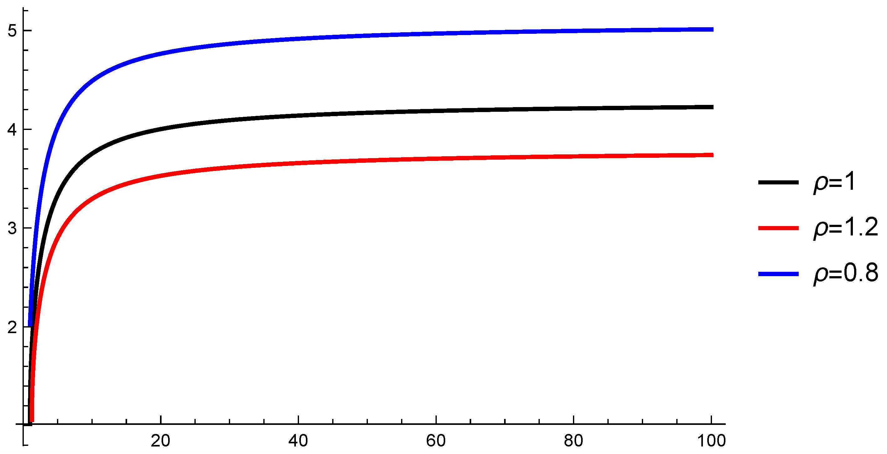
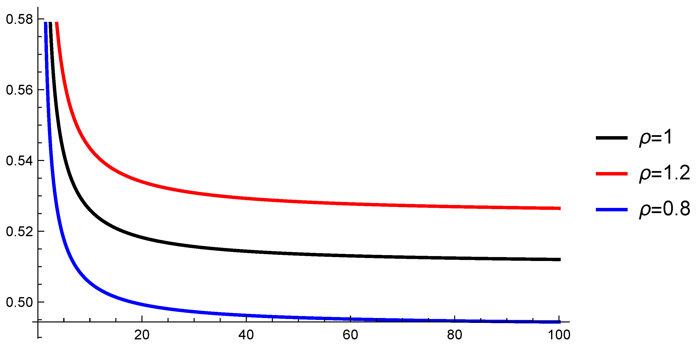
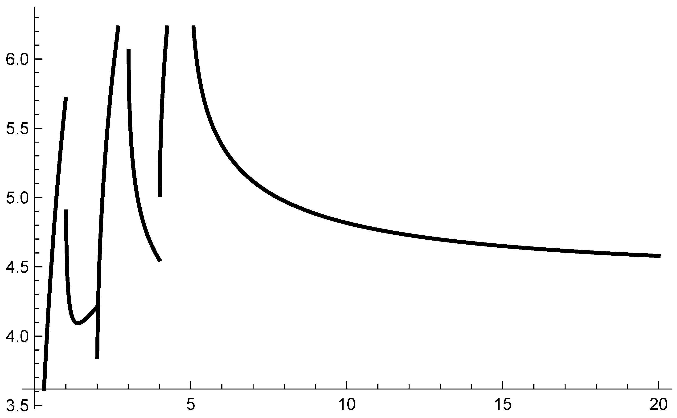
Let a = 1 , T < and q = 0.3 . The value of ρ > 0 does not change significantly the behavior of h ( t ) . However the type of the function ψ P ( 0 , T ) has a huge influence (see Figure 1 and Figure 2 with ψ ( t ) = e t P ( 0 , T ) and ψ = t t + 1 P ( 0 , T ) , respectively).
Consider the Mittag–Leffler function g ( t ) = E q ψ ( t ) ρ ( ψ ( a ) ) ρ ρ q with a = 1 , T < and q = 0.3 . If the function ψ ( t ) = e t P ( 0 , T ) , then the function g ( t ) approaches zero for any value of ρ (see Figure 3). If the function ψ = t t + 1 P ( 0 , T ) then the function g ( t ) decreases, but it does not approach zero (for example, if ρ = 1.2 then lim t g ( t ) = 0.47072 , see Figure 4).
Now consider the linear scalar fractional differential equation with GCFDF (5) with a = 1 , T < , q = 0.3 , ρ = 0.8 , u 0 = 1 , λ = 1 . According to Lemma 2 its solution is u ( t ) = E q ψ ( t ) ρ ( ψ ( 1 ) ) ρ ρ q , t [ 1 , T ] The solutions are increasing functions (see Figure 1 and Figure 2) but in the case ψ ( t ) = e t P ( 0 , T ) the solutions are approaching ∞. In the case ψ = t t + 1 P ( 0 , T ) , the solution is an increasing bounded function. Therefore, the applied function ψ in the fractional derivative has a huge influence on the behavior of the solutions.
Consider (5) with a = 1 , T < , q = 0.3 , ρ = 0.8 , u 0 = 1 , λ = 1 . According to Lemma 2 its solution is u ( t ) = E q ψ ( t ) ρ ( ψ ( 1 ) ) ρ ρ q , t [ 1 , T ] The solutions are decreasing functions (see Figure 1 and Figure 2) but in the case ψ ( t ) = e t P ( 0 , T ) the solutions are approaching 0. In the case ψ = t t + 1 P ( 0 , T ) , the solution is a decreasing function but not approaching 0.
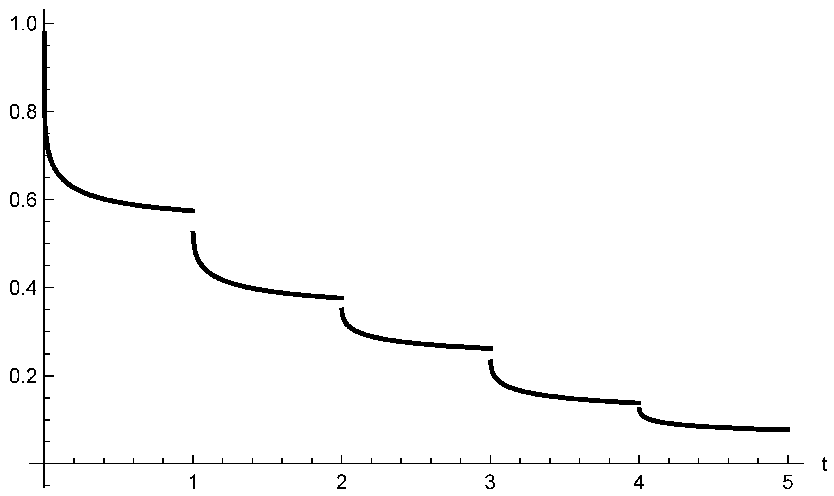
Now consider a switched linear scalar fractional differential equation with GCFDF. Let m = 5 and the subsystems are defined by (5) with a = 0 , q = 0.3 , ρ = 0.8 , u 0 = 1 , and various λ = ( 1 ) k where k is the number of the subsystem.
Let the switching times be ξ k = k , k = 1 , 2 , 3 , 4 , and the switching rule is σ ( t ) = k , t [ ξ k , ξ k + 1 ) , k = 1 , 2 , 3 , 4 , 5 .
Then the switching system will be
D a 0.3 , ψ 0.8 C u ( t ) = ( 1 ) k u ( t ) , f o r t ( ξ k , ξ k + 1 ] , k = 0 , 1 , 2 , 3 , 4 , D a q , ψ ρ C u ( t ) = u ( t ) , f o r t > ξ 5 , u ( 0 ) = 1 ,
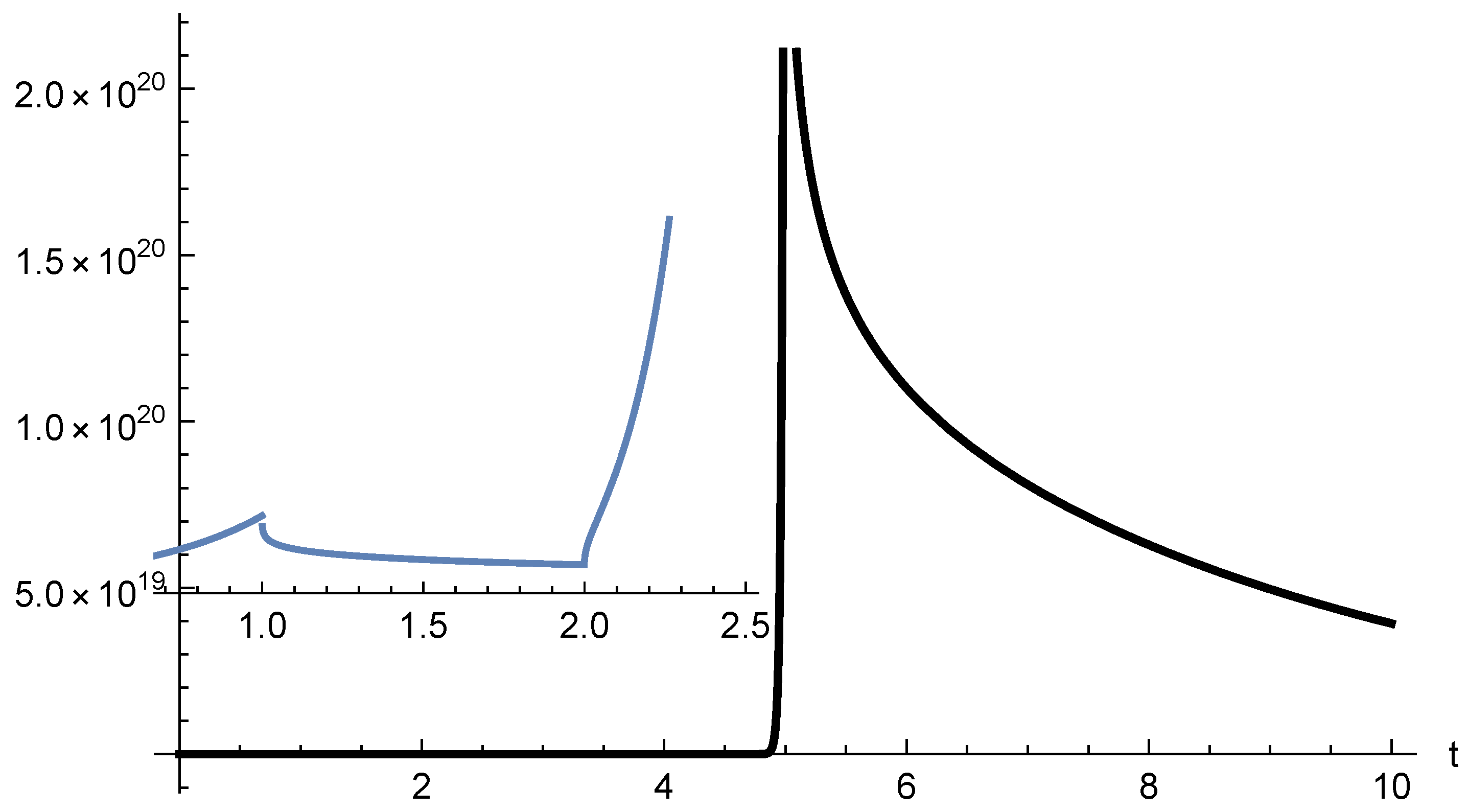
Consider the function ψ ( t ) = e t . The solution of the switched Equation (21) is given in Figure 5. It is seen that since the initial equation, defined by the first subsystem with λ = 1 is unstable, i.e., approaches infinity (see Figure 1), because of the switching rule, the solution could approach zero (see Figure 5).
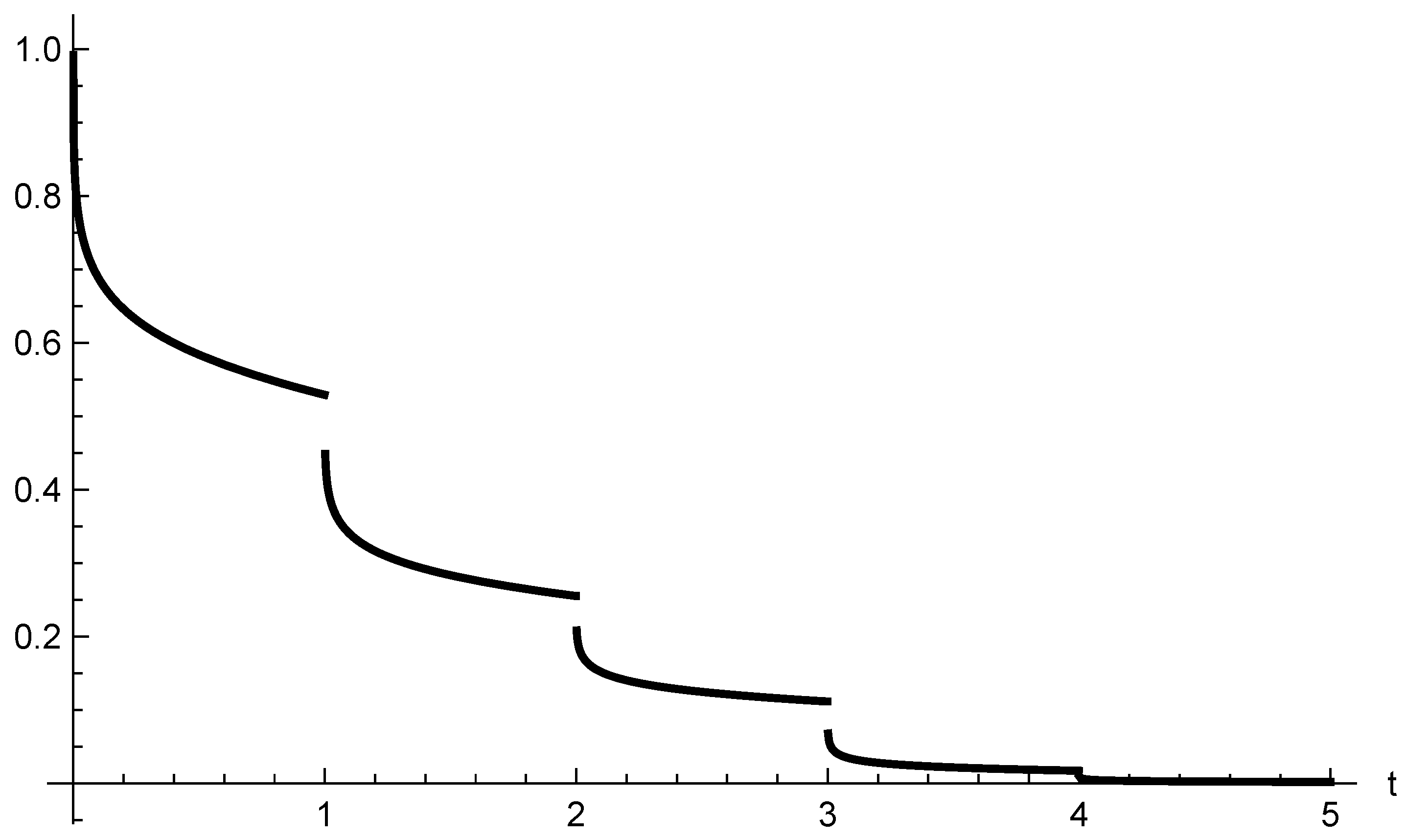
Consider the function ψ ( t ) = t t + 1 . The solution of the switched Equation (21) is given in Figure 6. It is seen that since the initial equation, defined by the first subsystem with λ = 1 , is increasing bounded (see Figure 2), because of the switching rule, the solution could be decreasing (see Figure 6).
Therefore, the above examples show that both the switching rule and the applied function in the fractional derivative can significantly change the behavior of the solution. It allows us to use the appropriate function ψ for the fractional derivative and the appropriate switching rule to adequately model the real situation studied in the neural network.
Remark 5.
Note the classical Caputo derivative is a special case of GCFDF with ψ ( t ) = t whose behavior is similar to the function ψ = e t , considered in Example 1, and the behavior of the solutions when the classical Caputo derivative is applied is similar to the case of ψ = e t and Figure 1, Figure 3 and Figure 5.
Now we will set up the switched studied model, and we will explain in detail its solution.
Consider the initial value problem (IVP) for the delay switched fractional Cohen–Grossberg neural network models with GCFDF (DSCDM):
D ξ k q , ψ ρ C u i ( t ) = d i ( u i ( t ) ) c i ( u i ( t ) ) j = 1 n a i j C k ( t ) f j C k ( u j ( t ) ) j = 1 n b i j C k ( t ) g j C k ( u j ( t h ( t ) ) ) I i , for t ( ξ k , ξ k + 1 ] , k M , i L u i ( θ ) = G i ( θ ) , θ [ μ , 0 ] , i L ,
where u ( t ) = ( u 1 ( t ) , u 2 ( t ) , , u N ( t ) ) T denotes the variable neuron’s state at time t; d i ( . ) , i L is the amplification function of the i-th neuron; c i ( . ) , i L is a well-behaved function; f j k ( . ) , g j k ( . ) , k M , j L are the activation functions of the j-th neuron; A k = { a i j k ( t ) } i , j L , B k = { b i j k ( t ) } i , j L , k M are neural connection memristive weights, C k M is the number of the neural connection memristive weights and the activation functions acting on the interval ( ξ k , ξ k + 1 ] ; G : [ μ , 0 ] R n is the initial function; I i is the external input; h : [ 0 , ) [ 0 , μ ] is the delay.
Remark 6.
If m < then the last interval ( ξ m 1 , ξ m ] in DSCDM (22) is changed to ( ξ m 1 , ) .
Remark 7.
If at a point ξ k , k = 1 , 2 , , m 1 , the equality C k 1 = C k holds, then the switching rule is not activated at the point ξ k , and the system is not changed, i.e., we have to ignore the point ξ k in DSCDM (22). By relabeling the points { ξ i } , we could obtain the case when C k 1 C k for all k = 1 , 2 , , m 1 and the switching rule is activated at all points ξ k , k = 1 , 2 , , m 1 .
According to Remark 7, without loss of generality, we assume that C k 1 C k for all k = 1 , 2 , , m 1 .
In this paper, we will use the following assumption:
(A).
For any k M and any initial function Φ C ( [ μ , 0 ] , R N ) , Φ = ( Φ 1 , Φ 2 , , Φ N ) , the delay fractional Cohen–Grossberg neural networks model (DCDM)
D ξ k q , ψ ρ C u i ( t ) = d i ( u i ( t ) ) ( c i ( u i ( t ) ) j = 1 n a i j C k ( t ) f j C k ( u j ( t ) ) j = 1 n b i j C k ( t ) g j C k ( u j ( t h ( t ) ) ) I i ) , for t ( ξ k , ξ k + 1 ] , k M , i L u i ( ξ k + θ ) = Φ i ( θ ) , θ [ μ , 0 ] , i L
has a solution u C q ( [ ξ k , ξ k + 1 ] , R N , ψ , ρ ) C ( [ ξ k h , ξ k ] , R N ) .
We will give a detailed description of the DSCDM (22), assuming condition (A) holds.
Let t [ ξ 0 , ξ 1 ] . Since σ ( s ) = 0 , s [ 0 , ξ 1 ] , the DSCDM (22) reduces to the following DCDM
D 0 q , ψ ρ C u i ( t ) = d i ( u i ( t ) ) c i ( u i ( t ) ) j = 1 n a i j 0 ( t ) f j 0 ( u j ( t ) ) j = 1 n b i j 0 ( t ) g j 0 ( u j ( t h ( t ) ) ) I i , for t ( 0 , ξ 1 ] , i L u i ( θ ) = G i ( θ ) , θ [ μ , 0 ] , i L .
According to assumption (A) with C k = 0 and Φ i ( t ) = G i ( t ) for t [ μ , 0 ] , DCDM (23) has a solution u ( 0 ) ( t ) C q ( [ 0 , ξ 1 ] , R N , ψ , ρ ) C ( [ μ , 0 ] , R N ) .
At time ξ 1 , the switching rule σ ( t ) is activated and the system of equations is changed, i.e., since σ ( t ) = C 1 M on [ ξ 1 , ξ 2 ) , the DSCDM (22) is reduced to the following DCDM
D ξ 1 q , ψ ρ C u i ( t ) = d i ( u i ( t ) ) c i ( u i ( t ) ) j = 1 n a i j C 1 ( t ) f j C 1 ( u j ( t ) ) j = 1 n b i j C 1 ( t ) g j C 1 ( u j ( t h ( t ) ) ) I i , for t ( ξ 1 , ξ 2 ] , i L u i ( θ ) = u i ( 0 ) ( θ ) , θ [ ξ 1 μ , ξ 1 ] , i L .
According to assumption (A) with C k = C 1 and Φ i ( t ) = u i ( 0 ) ( t ) for t [ μ , 0 ] , DCDM (24) has a solution u ( 1 ) ( t ) C q ( [ ξ 1 , ξ 2 ] , R N , ψ , ρ ) C ( [ ξ 1 μ , ξ 1 ] , R N ) .
From the second equation of (24), i.e., u i ( θ ) = u i ( 0 ) ( θ ) , θ [ ξ 1 μ , ξ 1 ] , it follows that u i ( 1 ) ( ξ 1 ) = u i ( 0 ) ( ξ 1 ) , i L . Therefore, the solution of DSCDM (22) is continuous at ξ 1 .
At time ξ 2 , the switching rule σ ( t ) = C 2 M is activated, and the system of equations is changed, i.e., DSCDM (22) is reduced to the following DCDM
D ξ 2 q , ψ ρ C u i ( t ) = d i ( u i ( t ) ) c i ( u i ( t ) ) j = 1 n a i j C 2 ( t ) f j C 2 ( u j ( t ) ) j = 1 n b i j C 2 ( t ) g j C 2 ( u j ( t h ( t ) ) ) I i , for t ( ξ 2 , ξ 3 ] , i L u i ( θ ) = u i ( 1 ) ( θ ) , θ [ ξ 2 μ , ξ 2 ] , i L .
According to assumption (A) with C k = C 2 and Φ i ( t ) = u i ( 1 ) ( t ) for t [ μ , 0 ] , DCDM (25) has a solution u ( 2 ) ( t ) C q ( [ ξ 2 , ξ 3 ] , R N , ψ , ρ ) C ( [ ξ 2 μ , ξ 2 ] , R N ) .
From the second equation of (25), i.e., u i ( θ ) = u i ( 1 ) ( θ ) , θ [ ξ 2 μ , ξ 2 ] , it follows that u i ( 2 ) ( ξ 2 ) = u i ( 1 ) ( ξ 2 ) , i L . Therefore, the solution of DSCDM (22) is continuous at ξ 2 .
Continue this process for any k M we obtain the solution of DSCDM (22)
-
for m < ,
u ( t ) = u ( 0 ) ( t ) , for t [ 0 , ξ 1 ] , u ( 1 ) ( t ) , for t ( ξ 1 , ξ 2 ] u ( 2 ) ( t ) , for t ( ξ 2 , ξ 3 ] u ( m 1 ) ( t ) , for t ( ξ m 1 , ] ;
-
for m = ,
u ( t ) = u ( 0 ) ( t ) , for t [ 0 , ξ 1 ] , u ( 1 ) ( t ) , for t ( ξ 1 , ξ 2 ] u ( 2 ) ( t ) , for t ( ξ 2 , ξ 3 ] .
Remark 8.
The equalities u i ( θ ) = u i ( k 1 ) ( θ ) , θ [ ξ k μ , ξ k + 2 ] , k M , show that u i ( k ) ( ξ k ) = u i ( k 1 ) ( ξ k ) , i L , k M . Therefore, the solution u ( t ) of DSCDM (22) is continuous at any switching time ξ k , k = 1 , 2 , 3 , . Also, for any k = 1 , 2 , , m 1 the equality u ( k ) ( θ ) = u ( k 1 ) ( θ ) holds for θ [ ξ k h , ξ k ] .
Define the set
C ξ q ( [ 0 , ) , ψ , ρ ) = i = 0 m 1 C q ( [ ξ i , ξ i + 1 ] , R N , ψ , ρ ) .
We consider the DSCDM (22) as a driven system and the following system as a response system (RDSCDM)
D ξ k q , ψ ρ C u i ( t ) = d i ( u i ( t ) ) ( c i ( u i ( t ) ) j = 1 n a i j C k ( t ) f j C k ( u j ( t ) ) j = 1 n b i j C k ( t ) g j C k ( u j ( t h ( t ) ) ) I i ) + Θ i C k ( t ) for t ( ξ k , ξ k + 1 ] , k M , i L u i ( θ ) = Ψ i ( θ ) , θ [ μ , 0 ] , i L ,
where Θ i C k ( t ) is the input continuous control on the interval t ( ξ k , ξ k + 1 ] , k M .
Let u C ξ q ( [ 0 , ) , R N , ψ , ρ ) C ( [ μ , 0 ] , R N ) and v C ξ q ( [ 0 , ) , R N , ψ , ρ ) C ( [ μ , 0 ] , R N ) be solutions of (22) and (28), respectively. Define the synchronization error e i ( t ) = u i ( t ) v i ( t ) , t μ , i L , and the control gains
Θ i C k ( t ) = T i C k e i ( t ) , for t ( ξ i , ξ i + 1 ] , i L , k M ,
where T i C k are constants.
We now introduce the following assumptions, which we will need in Theorem 1.
(H1).
The functions a i , j p , b i , j p C ( [ 0 , ) , R ) , i , j L , p M , and there exist positive numbers K p , K p , p M such that | a i , j p ( t ) | K p and | b i , j p ( t ) | K p for t 0 .
(H2).
There exist positive constants d ˜ i , d ^ i , i L , such that the amplification function satisfy the following:
0 < d ^ i d i ( x ) d ˜ i < , | d i ( y ) d i ( x ) | D i | y x | , x , y R , i L .
(H3).
For well behaved functions c i ( x ) and amplification functions d i ( x ) there exist positive constants A i , such that
d i ( y ) c i ( y ) d i ( x ) c i ( x ) y x A i , i L , x , y R , x y .
(H4).
All activation functions f ( k ) , g ( k ) C ( R , R ) , k M , are bounded, i.e., there exist constants S j k , S j k > 0 such that | f j k ( x ) | S j k , | g j k ( x ) | S j k , x R , j L , k M and are Lipschitzian with constants F j k , F j k > 0 , i.e.,
| f j k ( y ) f j k ( x ) | F j k | y x | , | g j k ( y ) g j k ( x ) | F j k | y x | , y , x R , j L , k M .
(H5)
Any solutions u , v C ξ q ( [ 0 , ) , R N , ψ , ρ ) C ( [ μ , 0 ] , R N ) of DSFDE (22) and RDSFDE (28), respectively, are such that u 2 , v 2 C ξ q ( [ 0 , ) , R N , ψ , ρ ) C ( [ μ , 0 ] , R N ) with u = ( u 1 , u 2 , , u N ) , u 2 = ( u 1 2 , u 2 2 , , u N 2 ) , v = ( v 1 , v 2 , , v N ) , v 2 = ( v 1 2 , v 2 2 , , v N 2 ) .
Remark 9.
Assumption (H1) guarantees the boundedness of the time variable coefficients of the activation functions, which is a natural restriction, and it does not allow the activation of neurons to be too big. Assumption (H2) concerns the amplification function, its positiveness, and the Lipschitz property (compare with [11]). Assumption (H3) is a standard assumption about well-behaved functions and amplification functions. Assumption (H4) concerns the activation functions. We consider the case of continuous, bounded, and Lipschitz activation functions. The strongest condition is (H5), which is connected with the application of the quadratic Lyapunov function. In most papers applying a quadratic Lyapunov function to study neural network models, this condition is missing, but not all solutions are quadratically differentiable, especially when a fractional derivative is used.

4. Main Results

4.1. Some Preliminary Results for Delay Switched Models with GCFDF

Lemma 6.
Assume the following:
1. 
The functions u , v C ξ q ( [ 0 , ) , R N , ψ , ρ ) C ( [ μ , 0 ] , R N ) are solution of DSFDE (22) and RDSFDE (28), respectively, such that u 2 , v 2 C ξ q ( [ 0 , ) , R N , ψ , ρ ) C ( [ μ , 0 ] , R N ) with u = ( u 1 , u 2 , , u N ) , u 2 = ( u 1 2 , u 2 2 , , u N 2 ) , v = ( v 1 , v 2 , , v N ) , v 2 = ( v 1 2 , v 2 2 , , v N 2 ) .
2. 
The function Λ C ( [ μ , 0 ] , ( 0 , 1 ] ) is such that for any t ( ξ k , ξ k + 1 ] , k M for which
max θ [ μ , 0 ] Λ ( θ ) i = 1 N e i 2 ( t + θ ) i = 1 N e i 2 ( t )
the inequality
D ξ k q , ψ ρ C i = 1 N e i 2 ( t ) λ C k i = 1 N e i 2 ( t )
holds where λ C k > 0 are constants, e i ( t ) = u i ( t ) v i ( t ) , t [ 0 , ) , i L , is the synchronization error.
  • Then
i = 1 N e i 2 ( t ) i = 1 N e i 2 ( 0 ) i = 0 k 1 E q λ C i ψ ( ξ i + 1 ) ρ ( ψ ( ξ i ) ) ρ ρ q × E q λ C k ψ ( t ) ρ ( ψ ( ξ k ) ) ρ ρ q f o r t ( ξ k , ξ k + 1 ] , k M .
Proof. 
We will use induction.
Consider the interval [ 0 , ξ 1 ] . From condition 2 for k = 0 and Corollary 2 with a = 0 , T = ξ 1 , n = N , x ( . ) = e ( . ) , λ = λ C 0 , we obtain
i = 1 N e i 2 ( s ) i = 1 N e i ( 0 ) 2 E q λ C 0 ψ ( s ) ρ ( ψ ( 0 ) ) ρ ρ q for all s [ 0 , ξ 1 ] .
Consider the interval ( ξ 1 , ξ 2 ] . From condition 2 for k = 1 , and Corollary 2 with a = ξ 1 , T = ξ 2 , n = N , x ( . ) = e ( . ) , λ = λ C 1 and inequality (33) for s = ξ 1 we obtain that
i = 1 N e i 2 ( s ) i = 1 N e i ( ξ 1 ) 2 E q λ C 1 ψ ( s ) ρ ( ψ ( ξ 1 ) ) ρ ρ q i = 1 N e i ( 0 ) 2 E q λ C 0 ψ ( ξ 1 ) ρ ( ψ ( 0 ) ) ρ ρ q E q λ C 1 ψ ( s ) ρ ( ψ ( ξ 1 ) ) ρ ρ q for all s [ ξ 1 , ξ 2 ] .
Following inductively this procedure we have inequality (32). □
Remark 10.
Condition 2 of Lemma 6 is a modified Razumikhin condition. Note, inequality (6) is not satisfied for all points t ( ξ k , ξ k + 1 ] , k M , but only for those satisfying the inequality (30). This is very important in the application of Lyapunov functions to study stability properties of any system with delays.

4.2. Global Mittag–Leffler Synchronization

Definition 3.
The DSCDM (22) and the RDSCDM (28) are globally Mittag–Leffler synchronized if there exist constants L p , p M , and K , β > 0 such that for any initial functions G , Ψ C ( [ μ , 0 ] , R N ) and any solutions x ( t ; G ) C ξ q ( [ 0 , ) , R N , ψ , ρ ) C ( [ μ , 0 ] , R N ) and y ( t ; Ψ ) C ξ q ( [ 0 , ) , R N , ψ , ρ ) C ( [ μ , 0 ] , R N ) of DSCDM (22) and RDSCDM (28), respectively, the inequality
| | x ( t ; G ) y ( t ; Ψ ) | | K | | G Ψ | | 0 E q L C k ψ ( t ) ρ ( ψ ( ξ k ) ) ρ ρ q β × j = 0 k 1 E q L C j ψ ( ξ j + 1 ) ρ ( ψ ( ξ j ) ) ρ ρ q β , t ( ξ k , ξ k + 1 ] , k M ,
holds, where | | x | | = i = 1 N x i 2 , x R N , x = ( x 1 , x 2 , , x N ) .
The continuous state feedback controller Θ ( t ) , defined by (29), will be designed to enable the controlled models (22) and (28) to synchronize.
Theorem 1.
Suppose the following conditions are fulfilled:
1. 
Assumptions (A), (H1)–(H5) are satisfied.
2. 
The constants T i p , i L , p M , in the state feedback controller defined by (29) is such that for any p M the inequalities
2 D i | I i | + 2 T i p + K p ( D i j = 1 N S j p + S j p + d ˜ i j = 1 N F j p + F j p + F i p j = 1 N d ˜ j ) + K p max i I F i p k = 1 N d ˜ k 2 A i γ p , i I
hold where γ p ( 0 , 2 min i I A i ] , p M is a constant.
Then the driven system (22) and the response system (28) are globally Mittag–Leffler synchronized under the control (29).
Proof. 
Let the initial functions G , Ψ C ( [ μ , 0 ] , R N ) . From condition (A) and the description of the solutions in Section 4.1 there exists a solution u C ξ q ( [ 0 , ) , R N , ψ , ρ ) C ( [ μ , 0 ] , R N ) of DSCDM (22) and a solution v C ξ q ( [ 0 , ) , R N , ψ , ρ ) C ( [ μ , 0 ] , R N ) of RDSCDM (28) with the given initial functions G , Ψ . The synchronization error is e C ( [ μ , 0 ] , R N ) : e ( t ) = u ( t ) v ( t ) .
Let t ( ξ k , ξ k + 1 ] , k M be a point such that
sup θ [ μ , 0 ] i + 1 N e i 2 ( t + θ ) i = 1 N e i 2 ( t ) .
Then according to Lemma 4 with a = ξ k , T = ξ k + 1 and conditions (H2), (H3), and (H4) we get
D q , ρ ξ k C i = 0 N e i ( t ) 2 2 i = 1 N e i ( t ) ( D q , ρ ξ k C e i ) ( t ) = 2 i = 1 N e i ( t ) D α , ρ ξ k C u i ( t ) D α , ρ ξ k C v i ( t ) 2 i = 1 N A i + D i | I i | + T i C k e i 2 ( t ) + 2 i = 1 N e i ( t ) j = 1 N | a i j C k ( t ) | | d i ( v i ( t ) ) | f j C k ( v j ( t ) ) f j C k ( u j ( t ) ) + 2 i = 1 N e i ( t ) j = 1 N | a i j C k ( t ) | | d i v i ( t ) d i u i ( t ) | | f j C k ( u j ( t ) ) | + 2 i = 1 N e i ( t ) j = 1 N | b i j C k ( t ) | | d i ( v i ( t ) ) | g j C k ( v j ( t h ( t ) ) ) g j C k ( u j ( t h ( t ) ) ) + 2 i = 1 N e i ( t ) j = 1 N | b i j C k ( t ) | | d i v i ( t ) d i u i ( t ) | | g j C k ( u j ( t h ( t ) ) ) | 2 i = 1 N ( A i + D i | I i | + T i C k + j = 1 N | a i j C k ( t ) | D i S j C k + j = 1 N | b i j C k ( t ) | D i S j C k ) e i 2 ( t ) + 2 i = 1 N j = 1 N | a i j C k ( t ) | d ˜ i F j C k | e i ( t ) | | e j ( t ) | + 2 i = 1 N j = 1 N | b i j C k ( t ) | d ˜ i F j C k | e i ( t ) | | e j ( t h ( t ) ) | .
Apply condition (H1) and the inequality 2 a b a 2 + b 2 to (37) to obtain
D q , ρ ξ k C i = 0 N e i ( t ) 2 2 i = 1 N A i + D i | I i | + T i C k + j = 1 N | a i j C k ( t ) | D i S j C k + | b i j C k ( t ) | D i S j C k e i 2 ( t ) + i = 1 N j = 1 N | a i j C k ( t ) | d ˜ i F j C k + | b i j C k ( t ) | d ˜ i F j C k e i 2 ( t ) + i = 1 N j = 1 N | a i j C k ( t ) | d ˜ i F j C k e j 2 ( t ) + i = 1 N j = 1 N | b i j C k ( t ) | d ˜ i F j C k e j 2 ( t h ( t ) ) i = 1 N [ 2 A i + D i | I i | + T i C k + K C k ( D i j = 1 N S j C k + S j C k + d ˜ i j = 1 N F j C k + F j C k + F i C k j = 1 N d ˜ j ) ] e i 2 ( t ) + K C k max i I F i C k k = 1 N d ˜ k i = 1 N e i 2 ( t h ( t ) ) .
From the choice of the point t and inequality (38) we have
D q , ρ ξ k C i = 0 N e i ( t ) 2 i = 1 N [ 2 A i + D i | I i | + T i C k + K C k ( D i j = 1 N S j C k + S j C k + d ˜ i j = 1 N F j C k + F j C k + F i C k j = 1 N d ˜ j ) + K C k max i I F i C k k = 1 N d ˜ k ] e i 2 ( t ) γ C K j = 1 N e i 2 ( t ) .
From inequalities (36) and (39) it follows that condition 2 of Lemma 6 is satisfied with Λ 1 , λ C k = γ C k . Condition (H5) guarantees condition 1 of Lemma 6. According to Lemma 6 we have
i = 1 N e i 2 ( t ) i = 1 N e i 2 ( 0 ) i = 0 k 1 E q γ C i ψ ( ξ i + 1 ) ρ ( ψ ( ξ i ) ) ρ ρ q × E q γ C k ψ ( t ) ρ ( ψ ( ξ k ) ) ρ ρ q for t ( ξ k , ξ k + 1 ] , k M .
Therefore, the DSCDM (22) and the RDSCDM (28) are globally Mittag–Leffler synchronized with K = 1 , L C k = γ C k , β = 0.5 , and G ( Θ ) = u ( Θ ) , Ψ ( Θ ) = v ( Θ ) , Θ [ μ , 0 ] . □

5. Example

Let q = 0.3 , ρ = 0 , 8 .
Let the switching time be ξ i = i , i = 1 , 2 , , m = 3 , i.e., three Cohen–Grossberg neural network models with different neural-connection memristive weights and different activation functions are given. The switching rule σ ( t ) = C k for t [ ξ k , ξ k + 1 ) , k = 1 , 2 , will switch at initially given times between these three different models to describe the situation more adequately. Let N = 4 , i.e., four neurons are in the network. Let C 3 k = 2 , C 3 k + 1 = 0 and C 3 k + 2 = 1 .
Let the delay h ( t ) = e t , t 0 , and the activation functions be f 1 k = f 2 k = f 3 k = f 4 k = f k , k = 0 , 1 , 2 and g 1 k = g 2 k = g 3 k = g 4 k = g k , k = 0 , 1 , 2 , where
f 0 ( u ) = 0.1 u 2 u 2 + 1 , f 1 ( u ) = 0.1 u 2 u 2 + 10 , f 2 ( u ) = 0.1 u 2 u 2 + 50 g 0 ( u ) = 0.1 e u e u e u + e u , g 1 ( u ) = 0.1 e u 10 e u e u + e u , g 2 ( u ) = 0.1 e u 0.1 e u e u + e u , u R .
Therefore, μ = 1 , S i k = 0.1 , i = 1 , 2 , 3 , 4 , k = 0 , 1 , 2 , F i 0 = 0.066 , F i 1 = 0.021 , F i 2 = 0.01 and S i k = 0.1 , i = 1 , 2 , 3 , 4 , k = 0 , 2 , S i 2 = 1 , i = 1 , 2 , 3 , 4 F i 0 = 0.1 , F i 1 = 0.56 , F i 2 = 0.055 ,   i = 1 , 2 , 3 , 4 . Let q = 0.3 , ρ = 0.8 .
Let I i = 0 and the functions | a i j k ( t ) | K k = 0.1 , | a i j k ( t ) | K k = 0.2 , i , j = 1 , 2 , 3 , 4 , k = 0 , 1 , 2 , t 0 .
Let c i ( u ) = 1.5 u + sin ( u ) , i = 1 , 2 , 3 , 4 , d i ( u ) = 1 + 1 1 + u 2 , i = 1 , 2 , 3 , 4 , with d ^ i = 1 , d ˜ i = 2 and D i = 0.67 . Then d i ( y ) c i ( y ) d i ( x ) c i ( x ) y x = ( 1 + 1 1 + y 2 ) ( 1.5 y + sin ( y ) ) ( 1 + 1 1 + x 2 ( 1.5 x + sin ( x ) ) y x A i = 5 .
Case 1. Let ψ ( u ) = e u P ( 0 , ) be the function in the applied GCFDF.
Let the control gain be Θ i p ( t ) = T i p e i ( t ) = T e i ( t ) , i = 1 , 2 , 3 , 4 , p = 0 , 1 , 2 , with T = 4 .
Thus, the inequalities (35) are reduced to
8 + 0.1 ( 0.67 j = 1 , 2 , 3 , 4 0.1 + 0.1 + 2 j = 1 , 2 , 3 , 4 0.066 + 0.1 + 0.066 j = 1 , 2 , 3 , 4 2 ) + 0.2 0.1 k = 1 , 2 , 3 , 4 2 8.38848 10 γ , 8 + 0.1 ( 0.67 j = 1 , 2 , 3 , 4 0.1 + 1 + 2 j = 1 N 0.021 + 0.1 + 0.021 j = 1 , 2 , 3 , 4 2 ) + 0.2 0.1 k = 1 , 2 , 3 , 4 2 7.7516 10 γ , 8 + 0.1 ( 0.67 j = 1 , 2 , 3 , 4 0.1 + 0.1 + 2 j = 1 , 2 , 3 , 4 0.01 + 0.055 + 0.01 j = 1 , 2 , 3 , 4 2 ) + 0.2 0.055 k = 1 , 2 , 3 , 4 2 8.2736 10 γ ,
with γ = 1.5 .
Therefore, the conditions of Theorem 1 are satisfied and then the driven system (22) and its corresponding response system (28) in this special case are globally Mittag–Leffler synchronized under the defined above control, i.e., the inequality
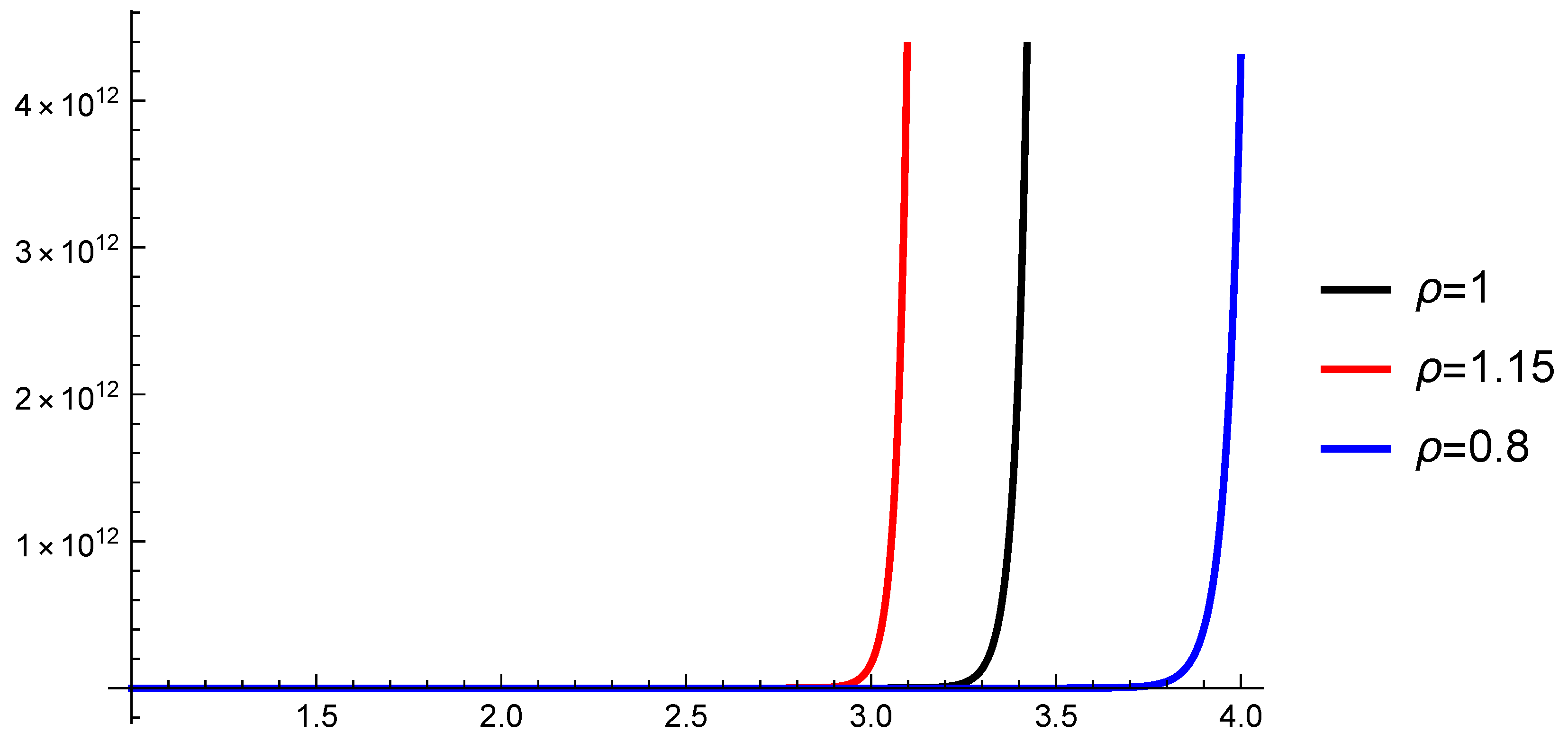
x ( t ) y ( t ) = i = 1 4 ( x ( t ) y ( t ) ) 2 = max θ [ 1 , 0 ] i = 1 4 ( x i ( θ ) y i ( θ ) ) 2 i = 0 k 1 E 0.3 1.5 2 0.3 1 e 0.5 0.3 e 0.15 i × E 0.3 1.5 2 0.3 e 0.5 t e 0.5 k 0.3 , t ( k , k + 1 ] , k = 0 , 1 , 2 ,
holds where x ( . ) is a solution of the driven system (22) and y ( . ) is a solution of the corresponding response system (28).
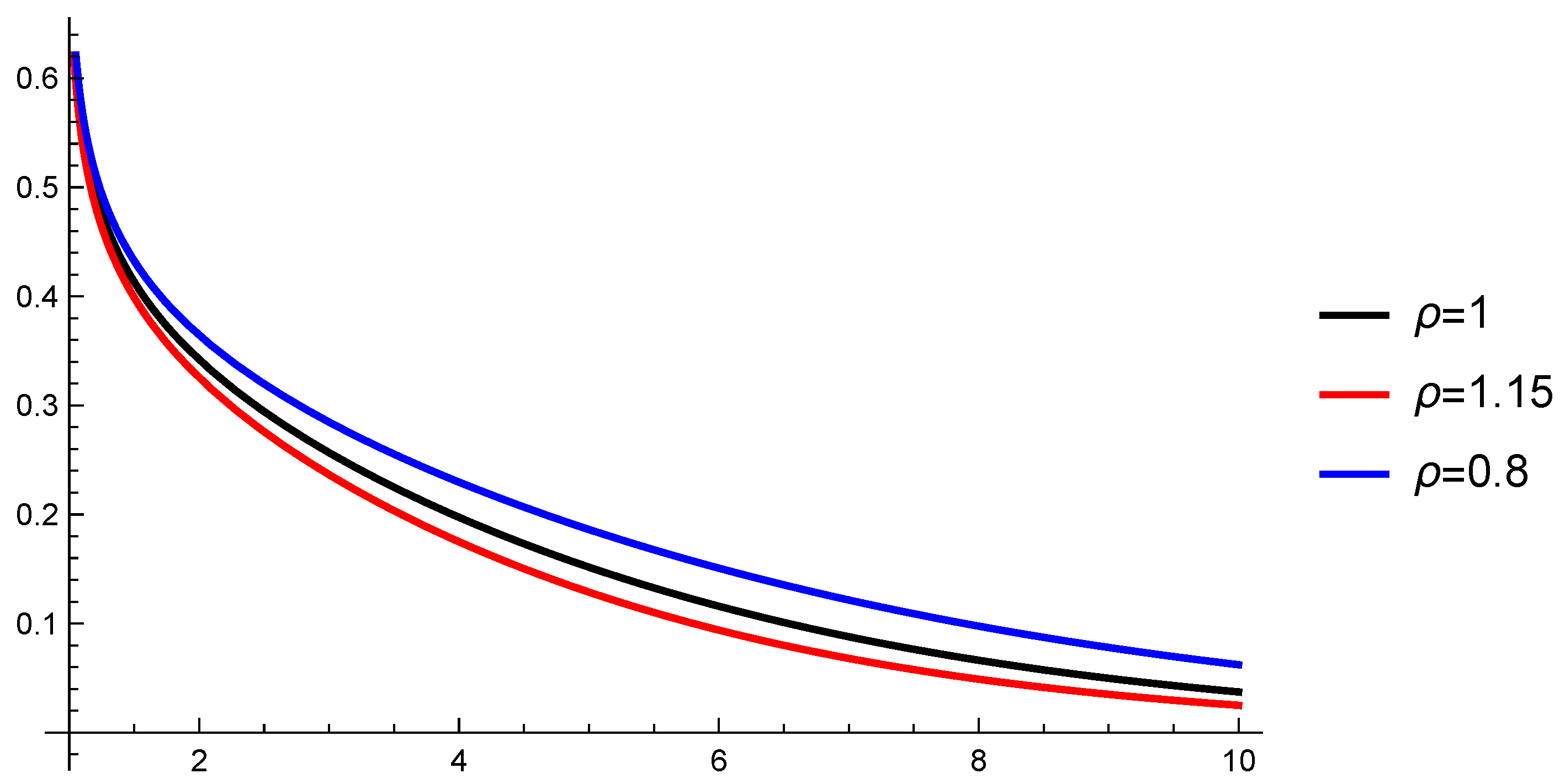
The graph of the estimate (42) of i = 1 4 ( x ( t ) y ( t ) ) 2 with
max θ [ 1 , 0 ] i = 1 4 ( x i ( θ ) y i ( θ ) ) 2 = 1
is given in Figure 7.
Case 2. Let ψ ( u ) = u u + 1 P ( 0 , ) be the function in the applied GCFDF.
Then, similar to Case 1, the conditions of Theorem 1 are satisfied and then the driven system (22) and its corresponding response system (28) in this special case are globally Mittag–Leffler synchronized under the defined above control, i.e., the inequality
x ( t ) y ( t ) = i = 1 4 ( x ( t ) y ( t ) ) 2 = max θ [ 1 , 0 ] i = 1 4 ( x i ( θ ) y i ( θ ) ) 2 i = 0 k 1 E 0.3 1.5 2 0.3 ( i + 1 i + 2 ) 0.8 ( i i + 1 ) 0.8 0.8 0.3 × E 0.3 1.5 2 0.3 ( t t + 1 ) 0.8 ( k k + 1 ) 0.8 0.8 0.3 , t ( k , k + 1 ] , k = 0 , 1 , 2 ,
holds where x ( . ) is a solution of the driven system (22) and y ( . ) is a solution of the corresponding response system (28).
The graph of the estimate (43) of i = 1 4 ( x ( t ) y ( t ) ) 2 with
max θ [ 1 , 0 ] i = 1 4 ( x i ( θ ) y i ( θ ) ) 2 = 1
is given in Figure 8.
6. Conclusions

In this paper, a delay switched memristive fractional Cohen–Grossberg neural network is considered. The switched rule allows us to use one of the initially given sets of models with different activation functions. The switching times are specified initially and determine not only the model switching times but also the lower bounds of the applied fractional derivatives. To be more general, we consider the generalized Caputo fractional derivative with respect to another function. We consider a continuous controller, define generalized Mittag–Leffler synchronization, and obtain some sufficient conditions. The results are significant for various applications in engineering and technology. The above example illustrates that if all models in the initially given set are Mittag–Leffler synchronized, then a switching rule that changes one model at certain moments to another preserves the property.
It would be interesting to extend our results to the various switching models of neural networks. This topic goes beyond the scope of this paper and will be a challenging issue for future research.

Author Contributions

Conceptualization, D.O. and S.H.; methodology, D.O. and S.H.; formal analysis, D.O. and S.H.; writing—original draft preparation, D.O. and S.H.; writing—review and editing, D.O. and S.H. All authors have read and agreed to the published version of the manuscript.

Funding

The research was partially funded by the Bulgarian National Science Fund under Project KP-06-N62/1.

Institutional Review Board Statement

Not applicable.

Informed Consent Statement

Not applicable.

Data Availability Statement

The original contributions presented in this study are included in the article. Further inquiries can be directed to the corresponding author.

Conflicts of Interest

The authors declare no conflicts of interest.

References

  1. Zhang, W.; Wu, R.; Cao, J.; Alsaedid, A.; Hayat, T. Synchronization of a class of fractional-order neural networks with multiple time delays by comparison principles. Nonlinear Anal. Modell. Control 2017, 22, 636–645. [Google Scholar] [CrossRef]
  2. Hu, T.; He, Z.; Zhang, X.; Zhong, S. Global synchronization of time-invariant uncertainty fractional-order neural networks with time delay. Neurocomputing 2019, 339, 45–58. [Google Scholar] [CrossRef]
  3. Rifhat, R.; Muhammadhaji, A.; Teng, Z. Global Mittag–Leffler synchronization for impulsive fractional-order neural networks with delays. Intern. J. Nonlinear Sci. Numer. Simul. 2018, 19, 205–213. [Google Scholar] [CrossRef]
  4. Ding, X.; Cao, J.; Zhao, X.; Alsaadi, E. Mittag–Leffler synchronization of delayed fractional-order bidirectional associative memory neural networks with discontinuous activations: State feedback control and impulsive control schemes. Proc. A 2017, 473, 20170322. [Google Scholar] [CrossRef] [PubMed]
  5. Jebril, I.H.; Batiha, I.M.; Momani, S.; Biswas, A. Control Strategies for Mittag–Leffler Synchronization in Variable-Order Fractional Fitz Hugh-Nagumo Reaction-Diffusion Networks. Contemp. Math. 2026, 6, 6414–6443. [Google Scholar]
  6. Stamova, I.; Stamov, G. Mittag–Leffler synchronization of fractional neural networks with time-varying delays and reaction-diffusion terms using impulsive and linear controllers. Neural Netw. 2017, 96, 22–32. [Google Scholar] [CrossRef] [PubMed]
  7. Wang, G.; Ding, Z.; Li, S.; Yang, L.; Jiao, R. Finite-time Mittag–Leffler synchronization of fractional-order complex-valued memristive neural networks with time delay. Chin. Phys. B 2022, 31, 100201. [Google Scholar] [CrossRef]
  8. Agarwal, R.; Hristova, S.; O’Regan, D. Global Mittag–Leffler synchronization for neural networks modeled by impulsive Caputo fractional differential equations with distributed delays. Symmetry 2018, 10, 473. [Google Scholar] [CrossRef]
  9. Yazhini, M.; Samidurai, R. Global Mittag–Leffler synchronization of fractional-order complex-valued BAM neural networks with linear feedback controllers. Int. J. Dynam. Control 2025, 13, 398. [Google Scholar] [CrossRef]
  10. Fan, Y.; Huang, X.; Wang, Z.; Xia, J.; Li, Y. Global Mittag–Leffler synchronization of delayed fractional-order memristive neural networks. Adv. Differ. Equ. 2018, 2018, 338. [Google Scholar] [CrossRef]
  11. Cohen, M.A.; Grossberg, S. Absolute stability and global pattern formation and parallel memory storage by competitive neural networks. IEEE Trans. Syst. Man Cybern. 1983, SMC-13, 815–821. [Google Scholar] [CrossRef]
  12. Hopfield, J.J. Neurons with graded response have collective computational properties like those of two-stage neurons. Proc. Natl. Acad. Sci. USA 1984, 81, 3088–3092. [Google Scholar] [CrossRef] [PubMed]
  13. Zhang, L.; Yang, Y.; Xu, X. Synchronization analysis for fractional order memristive Cohen–Grossberg neural networks with state feedback and impulsive control. Phys. A Stat. Mech. Appl. 2018, 506, 644–660. [Google Scholar] [CrossRef]
  14. Kao, Y.; Cao, Y.; Chen, X. Global Mittag–Leffler synchronization of coupled delayed fractional reaction-diffusion Cohen–Grossberg neural networks via sliding mode control. Chaos 2022, 32, 113123. [Google Scholar] [CrossRef] [PubMed]
  15. Almeida, R. A Caputo fractional derivative of a function with respect to another function. Commun. Nonl. Sci. Numer. Simul. 2017, 44, 460–481. [Google Scholar] [CrossRef]
  16. Agarwal, R.; Hristova, S.; O’Regan, D. Cohen–Grossberg neural network delay models with fractional derivatives with respect to another function-Theoretical bounds of the solutions. Axioms 2024, 13, 605. [Google Scholar] [CrossRef]
  17. Nieto, J.J.; Alghnmi, M.; Ahmad, B.; Alsaedi, A.; Alharbi, B. On fractional integrals and derivatives of a functions with respect to another function. Fractals 2023, 31, 2340066. [Google Scholar] [CrossRef]
  18. Agarwal, R.P.; Hristova, S.; O’Regan, D. Stability of nonlinear switched fractional differential equations with short memory. Fractal Fract. 2025, 9, 598. [Google Scholar] [CrossRef]
  19. Sayed, W.S.; Henein, M.R.; Abd-El-Hafiz, S.K.; Radwan, A.G. Generalized dynamic switched synchronization between combinations of fractional-order chaotic systems. Complexity 2017, 2017, 9189120. [Google Scholar] [CrossRef]
  20. Pan, G.; Pang, D.; Liu, S. Synchronization analysis of fractional delayed dynamical networks under switching topology. Phys. Scr. 2025, 100, 025218. [Google Scholar] [CrossRef]
Figure 1. Graph of the function E 0.3 ( ( e t ρ e ρ ρ ) 0.3 ) .
Mathematics 14 00726 g001
Figure 2. Graph of the function E 0.3 ( t t + 1 1 2 ) ρ ρ 0.3 .
Mathematics 14 00726 g002
Figure 3. Graph of the function E 0.3 ( ( e t ρ e ρ ρ ) 0.3 ) .
Mathematics 14 00726 g003
Figure 4. Graph of the function E 0.3 ( t t + 1 1 2 ) ρ ρ 0.3 .
Mathematics 14 00726 g004
Figure 5. Graph of the solution of (21) with ψ ( t ) = e t .
Mathematics 14 00726 g005
Figure 6. Graph of the solution of (21) with ψ ( t ) = t t + 1 .
Mathematics 14 00726 g006
Figure 7. Graph of the estimate of (42) with ψ ( t ) = e t .
Mathematics 14 00726 g007
Figure 8. Graph of the estimate (43) with ψ ( t ) = t t + 1 .
Mathematics 14 00726 g008
Disclaimer/Publisher’s Note: The statements, opinions and data contained in all publications are solely those of the individual author(s) and contributor(s) and not of MDPI and/or the editor(s). MDPI and/or the editor(s) disclaim responsibility for any injury to people or property resulting from any ideas, methods, instructions or products referred to in the content.