Intelligent Inversion of Deep In Situ Stress Fields Based on the ABC-SVR Algorithm

Abstract

Accurate inversion of the deep initial in situ stress field is a fundamental prerequisite for stability analysis of surrounding rock in underground engineering, roadway support design, and prevention and control of dynamic disasters. To address the problems of scarce in situ stress measurements in deep mining areas, the inability of conventional regression methods to capture the nonlinear characteristics of complex tectonic stress fields, and the tendency of traditional inversion algorithms to fall into local optima and overfitting, this paper proposes an intelligent inversion method based on support vector regression optimized by the artificial bee colony algorithm (ABC-SVR). The artificial bee colony algorithm is employed to adaptively optimize the core parameters of the SVR model, thereby enabling high-precision inversion of complex deep stress fields. Comparing the results with acoustic emission tests demonstrated that the ABC-SVR model significantly outperforms conventional SVR and backpropagation neural networks across various performance metrics. The inversion results show high consistency with the measured data, achieving a root mean square error (RMSE) of 1.25, a mean absolute percentage error (MAPE) of 4.16%, and a coefficient of determination (R²) of 0.908. This method can rapidly reconstruct high-precision initial in situ stress fields in deep unmined regions, providing highly reliable boundary conditions for numerical simulations and demonstrating significant engineering application potential.

1. Introduction

Deep in situ rock stress is a fundamental prerequisite for mining scheme design, parameter determination, ground pressure analysis, and safety monitoring. This is particularly critical for deep mining areas characterized by high tectonic stress fields, as the stress state directly impacts the stability of underground engineering structures and the surrounding rock [1,2,3]. At present, the mining depth of many mines worldwide exceeds 1000 m or even greater. For instance, the maximum mining depth of the Mponeng Gold Mine in South Africa has surpassed 4000 m, and the Kidd Creek Mine in Canada reaches approximately 3000 m deep [4]. Similarly, several mines in China, such as the Hongtoushan Copper Mine and the Dongguashan Copper Mine, have also exceeded a depth of 1000 m [5]. With increasing mining depth, the challenges of high in situ stress, high temperature, and strong mining disturbance have become prominent [6,7,8]. Under such deep, high-stress conditions, disturbances caused by mining operations can easily trigger accidents such as rockburst and roof collapses [9,10,11]. The reconstruction of in situ stress field provides not only boundary conditions for numerical simulation, but also a critical basis for practical stress control and pressure relief [12,13]. Consequently, accurately determining the distribution characteristics of in situ stress in deep mining areas is of paramount importance.

At present, the primary methods for obtaining in situ stress distribution data can be broadly classified into traditional field measurements and numerical inversion methods [14,15]. These field measurement techniques mainly include hydraulic fracturing, overcoring, and acoustic emission methods [16,17,18]. Although field measurements can accurately determine the stress state at specific monitoring points, they are associated with high costs, long implementation periods, and difficulties in deploying high-density measurement points over large, deep regions. Consequently, the resulting datasets are often sparse. However, relying solely on a limited number of discrete measurement points makes it difficult to accurately characterize the complex in situ stress field distribution of an entire mining area [19,20,21]. To overcome the limitations posed by scarce measured data, numerical inversion methods for in situ stress have been developed. These methods aim to reconstruct the in situ stress field using limited measurement points to accurately determine the stress distribution within underground rock masses. Early inversion methods predominantly employed multivariate linear regression analysis. By assuming a linear relationship between in situ stress and factors such as burial depth and spatial coordinates, these methods establish linear statistical models relating self-weight stress and tectonic stress [22,23]. For instance, Liang et al. [24] established a 3D geological model of a mining area and obtained the deep stress field through multivariate linear regression inversion. Chen et al. [25] analyzed the in situ stress characteristics near a tunnel fault zone using multivariate linear regression and FLAC^3D software. Li et al. [26] proposed an improved stress inversion method based on least squares regression, which effectively enhanced prediction accuracy in stress anomaly regions.

In recent years, driven by rapid advances in artificial intelligence and big data technologies, machine learning algorithms have been increasingly applied in the field of geotechnical engineering [27,28]. For instance, Zhang and Yin [29] determined horizontal in situ stress by coupling an artificial neural network (ANN) with a genetic algorithm (GA), utilizing data from hydraulic fracturing tests. Li et al. [30] obtained in situ stress field measurements by applying boundary loads using finite element software in combination with a backpropagation (BP) neural network and validated the results against those obtained from multivariate linear regression. In the Sejila region, Fu et al. [31] established the initial in situ stress field by combining numerical simulation with support vector regression (SVR). To address the nonlinear characteristics of the stress field around a hydropower station tunnel, Wang et al. [32] fused long short-term memory (LSTM) with an attention neural network, which significantly enhanced inversion accuracy. Li et al. [33] achieved an accurate in situ stress field measurement by optimizing the boundary conditions of numerical models using BP neural networks and a genetic algorithm (GA). Garavand and Hadavimoghaddam [34] employed four algorithms, including XGBoost, LightGBM, Catboost, and Adaboost, to estimate in situ stress combined with rock plastic behavior and compared the results of the four methods. Xiang et al. [35] developed a backpropagation neural network (BPNN)-based model to achieve high-precision prediction of the maximum and minimum horizontal principal stresses using cross-scale caving characteristics. Mustafa et al. [36] achieved high-precision prediction of in situ stress fields by integrating petrophysical theory with an integrated framework based on machine learning and deep learning.

Although previous studies have achieved fruitful results, a critical gap remains unresolved: how to achieve high-precision stress inversion with limited measured data and under complex geological conditions. Traditional multiple regression methods rely on linear assumptions and fail to capture the nonlinear characteristics of deep tectonic stress fields. In contrast, neural networks (e.g., BP-ANN) exhibit strong nonlinear mapping ability but are based on empirical risk minimization (ERM). However, datasets in deep mining engineering are usually small, which often leads to overfitting and trapping in local optima.

To address the engineering challenges of scarce in situ stress test samples and complex tectonic stress field distribution in the deep mining area of a certain mine, this paper proposes an intelligent inversion algorithm model for measuring in situ stress fields based on support vector regression (SVR) optimized with the artificial bee colony (ABC) algorithm. Traditional parameter selection methods for SVR (e.g., grid search) suffer from low computational efficiency and lack of global search capability. Therefore, the ABC algorithm is introduced to automatically identify the globally optimal parameters of SVR. This hybrid ABC-SVR strategy combines the small-sample robustness of SVR and the global optimization efficiency of ABC, ensuring accuracy and stability. Based on the geological characteristics of the study area, a three-dimensional numerical model was established. By integrating measured acoustic emission-based in situ stress data from key deep locations, a training sample library incorporating different boundary conditions was constructed using FLAC^3D numerical simulations. On this basis, the artificial bee colony algorithm was introduced to adaptively optimize the key parameters of the SVR model, thereby enhancing the generalization capability and fitting performance of the inversion model for nonlinear stress fields. This study is intended to provide a new theoretical method for refined inversion of in situ stress fields for deep areas with few samples and to offer reliable data support for the design of deep mining approaches and the prevention and control of dynamic disasters in mines.

2. Principle and Method of In Situ Stress Inversion

2.1. Support Vector Regression

Support vector machine (SVM) is a machine-learning method based on statistical learning theory [37]. SVM follows the principle of structural risk minimization (SRM), which minimizes the training error while maximizing the model margin to reduce the upper bound of the model’s generalization error. Therefore, SVM exhibits distinct advantages in addressing small-sample and nonlinear classification problems. Support vector regression (SVR) is the form of SVM applied to the field of regression prediction.

2.1.1. SVR Basic Model and ε-Insensitive Loss Function

Let the numerical simulation training sample set for in situ stress inversion be $T=\{(x_i,y_i)|i=1,2,\dots ,l\}$, where $x_i\in R^n$ denotes the input vector, $y_i\in R^n$ denotes the output target value, $l$ represents the number of samples. The goal of SVR is to find a nonlinear mapping $\varphi (x)$, which maps the low-dimensional space to a high-dimensional feature space, and then construct a linear regression function in this space

$$f(x)={\omega }^T\cdot \varphi (x)+b$$

(1)

where $\omega$ denotes the weight vector, $b$ denotes the bias term, and $\varphi (x)$ denotes the nonlinear mapping function that maps the input to the high-dimensional feature space.

To determine $\omega$ and $b$, SVR introduces the ε-insensitive loss function: when the deviation between the predicted value $f(x)$ and the true value y is less than ε, the loss is ignored; otherwise, the loss is calculated. Based on the SRM principle, the optimization problem of SVR can be formulated as minimizing the following objective function:

$${\min }_{\omega ,b,\xi ,{\xi }^{*}}{\displaystyle \frac{1}{2}}\Vert \omega {\Vert }^2+C{\displaystyle \sum _{i=1}^l\left({\xi }_i+{\xi }_i^{*}\right)}$$

(2)

The constraint conditions are

$$\left\{\begin{array}{l}{y}_i-\left({\omega }^T\cdot \varphi (x_i)+b\right)\le \epsilon +{\xi }_i\hfill \\ \left({\omega }^T\cdot \varphi (x_i)+b\right)-y_i\le \epsilon +{\xi }_i^{*}\hfill \\ {\xi }_i,{\xi }_i^{*}\ge 0, i=1,2,\dots ,l\hfill \end{array}\right.$$

(3)

where $\Vert \omega {\Vert }^2$ represents the complexity of the model: the smaller its value, the smoother the model. C is the Penalty Factor, which is used to balance the weight between model complexity and training error, and ${\xi }_i$ and ${\xi }_i^{*}$ are slack variables, which are used to tolerate the errors of some sample points exceeding ε.

2.1.2. Dual Problem and Kernel Function

Introduce Lagrange multipliers ${\alpha }_i$ and ${\alpha }_i^{*}$ and apply the Karush–Kuhn-–Tucker (KKT) conditions to convert the aforementioned primal optimization problem into a dual problem for resolution. The finally derived nonlinear regression function is expressed as follows:

$$f(x)={\displaystyle \sum _{i=1}^l\left({\alpha }_i-{\alpha }_i^{*}\right)}K(x_i,x)+b$$

(4)

where $K(x_i,x)=\varphi {(x_i)}^T\cdot \varphi (x)$ is the kernel function, which directly calculates the inner product of the high-dimensional space in the original space.

The radial basis function (RBF) kernel is adopted in this paper, owing to its strong nonlinear mapping capability and relatively few parameters:

$$K(x_i,x_j)=\exp (-\gamma \Vert x_i-x_j{\Vert }^2)$$

(5)

where γ is the kernel parameter, which controls the width of the distribution of samples in the feature space.

2.2. Artificial Bee Colony

The artificial bee colony (ABC) algorithm is a kind of swarm intelligence optimization algorithm proposed by Karaboga and Bastur [38]. By simulating the foraging behavior of bee colonies, this algorithm achieves global search of the solution space through information sharing and cooperation among individual bees [39].

2.2.1. Bee Colony Roles and Mechanisms

The artificial bee colony (ABC) algorithm divides the bee colony into three categories:

• Employed Bees: They are responsible for searching for food sources and recording their location information, and their number usually accounts for half of the total bee colony.
• Onlooker Bees: They stay inside the hive and select food sources to exploit with a certain probability according to the food source information shared by employed bees (usually via the waggle dance).
• Scout Bees: When a food source is not updated after multiple exploitation attempts (i.e., falling into a local optimum), the food source will be abandoned, and the corresponding employed bees will be transformed into scout bees to search for new food sources randomly.

2.2.2. Search Process

Assume the dimension of the solution space is D (in this study, D = 2, corresponding to C and γ), and the number of food sources is SN.

1.

Initialization Phase: Randomly generate SN initial solutions $X_i(i=1,\dots ,SN)$:

$$x_{ij}=x_{\min ,j}+\mathrm{rand}(0,1)(x_{\max ,j}-x_{\min ,j})$$

(6)

where $j\in \{1,\dots ,D\}$.

2.

Employed Bee Phase: Employed bees perform neighborhood search near the current food source $X_i$ to generate a new solution $V_i$:

$$v_{ij}=x_{ij}+{\varphi }_{ij}(x_{ij}-x_{kj})$$

(7)

where $k\in \{1,\dots ,SN\}$ is a randomly selected neighbor, and ${\varphi }_{ij}$ is a random number within [−1, 1]. If the fitness of the new solution $X_i$ is better than that of $V_i$, update greedily; otherwise, retain the original solution.

3.

Onlooker Bee Phase: Onlooker bees select food sources according to the probability $P_i$. The higher the fitness of a food source, the greater the probability of being selected:

$$P_i={\displaystyle \frac{fi{t}_i}{{\displaystyle \sum _{n=1}^{SN}f}i{t}_n}}$$

(8)

4.

Scout Bee Phase: If a food source has not been improved after a limited number of cycles, discard this solution, and the scout bee will randomly generate a new solution using the initialization formula.

2.3. ABC-SVR Algorithm

The prediction accuracy of the SVR model is highly dependent on the selection of two key parameters:

• Penalty factor C: Determines the model’s tolerance for training errors.
• Kernel parameter γ: Determines the distribution characteristics of data mapped to a high-dimensional space and the influence range of a single sample.

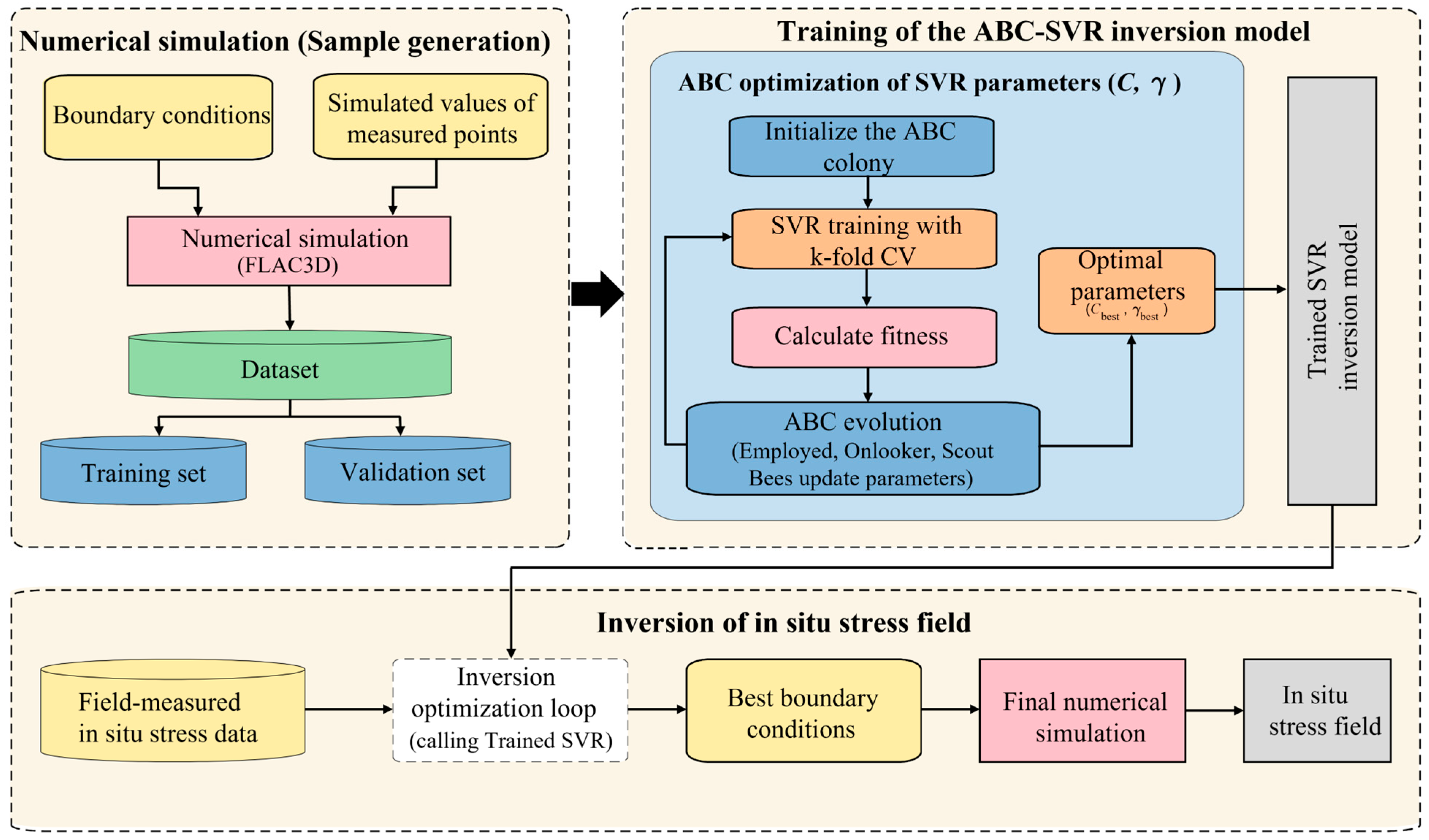
Due to the high nonlinearity of the deep in situ stress field and the scarcity of measured in situ stress samples, it is difficult to determine the optimal (C, γ) combination relying on manual experience or the trial-and-error method. Therefore, this study introduces the artificial bee colony (ABC) algorithm for adaptive parameter optimization. The ABC-SVR inversion model constructed in this study aims to automatically determine the optimal parameter combination of SVR through the global search capability of the ABC algorithm, so as to establish high-precision nonlinear mapping between boundary conditions and measured point stresses. The flowchart of the ABC-SVR algorithm is shown in Figure 1.

The specific steps for intelligent inversion of the in situ stress field using ABC-SVR are as follows:

• Based on the geological survey data of the engineering area, combined with the topographic and geomorphic conditions, use modeling software to establish a refined 3D geological model of the study area and determine the rock mass mechanical parameters.
• Refer to the results of historical in situ stress tests and supplementary in situ stress tests to obtain the general distribution law of the in situ stress field, determine the boundary condition parameters of the calculation model, and design multiple sets of orthogonal experimental schemes to make the boundary loads vary within a reasonable range.
• Take each set of constructed boundary conditions as the boundary conditions for one calculation simulation and obtain the calculated in situ stress values of the measured points corresponding to each set of boundary conditions.
• Use the artificial bee colony (ABC) algorithm to perform adaptive optimization on the parameters of the support vector regression (SVR) model, determine the optimal (C, γ) combination, and establish a high-precision intelligent inversion model.
• Extract the in situ stress values corresponding to the coordinates of the on-site measured points calculated under each combination of boundary conditions as the input values of the model network, and take the boundary conditions as the output values of the model network to train the model.
• Based on the optimal boundary conditions obtained by model inversion, substitute them into the model for forward calculation to obtain the in situ stress values of each measured point obtained by inversion.

3. Engineering Background and Data Acquisition

3.1. Engineering Overview

The mining area is located in a transitional slope zone between the Yunnan–Guizhou Plateau and the Guangxi Karst Basin, characterized by low-to-moderate mountainous terrain with shallow dissection, steep slopes, and well-developed gullies. The topography is high in the central part and low in the surrounding areas, and the geomorphology is of the structural erosion type. The mountain ranges generally strike in the northwest direction, with an elevation ranging from 760 m to 900 m, a relative height difference of 150 m to 200 m, a maximum peak elevation of 981 m, a minimum valley elevation of 620 m, and a slope gradient of 30° to 40°. With the extension of the mine’s service life, the main subsequent mining areas have gradually extended to depths below the −250 m level. As the mining depth increases, the problem of high in situ stress in deep rock masses has become increasingly prominent. Analysis of historical deep in situ stress test data shows that the lateral pressure coefficients in deep areas are all greater than 1, indicating that the horizontal tectonic stress in the deep part of this area is higher than the self-weight stress, which is characterized by a distinct tectonic stress field dominated by tectonic stress. Deep mining exerts significant disturbance on the in situ stress of the rock mass in the mining area, seriously disrupting the equilibrium state of the stress field in deep rock masses. This has led to frequent occurrences of goaf roof collapse and roadway caving accidents underground, and the intense ground pressure behavior poses a severe threat to the safety of deep mining operations.

3.2. In Situ Stress Measurement

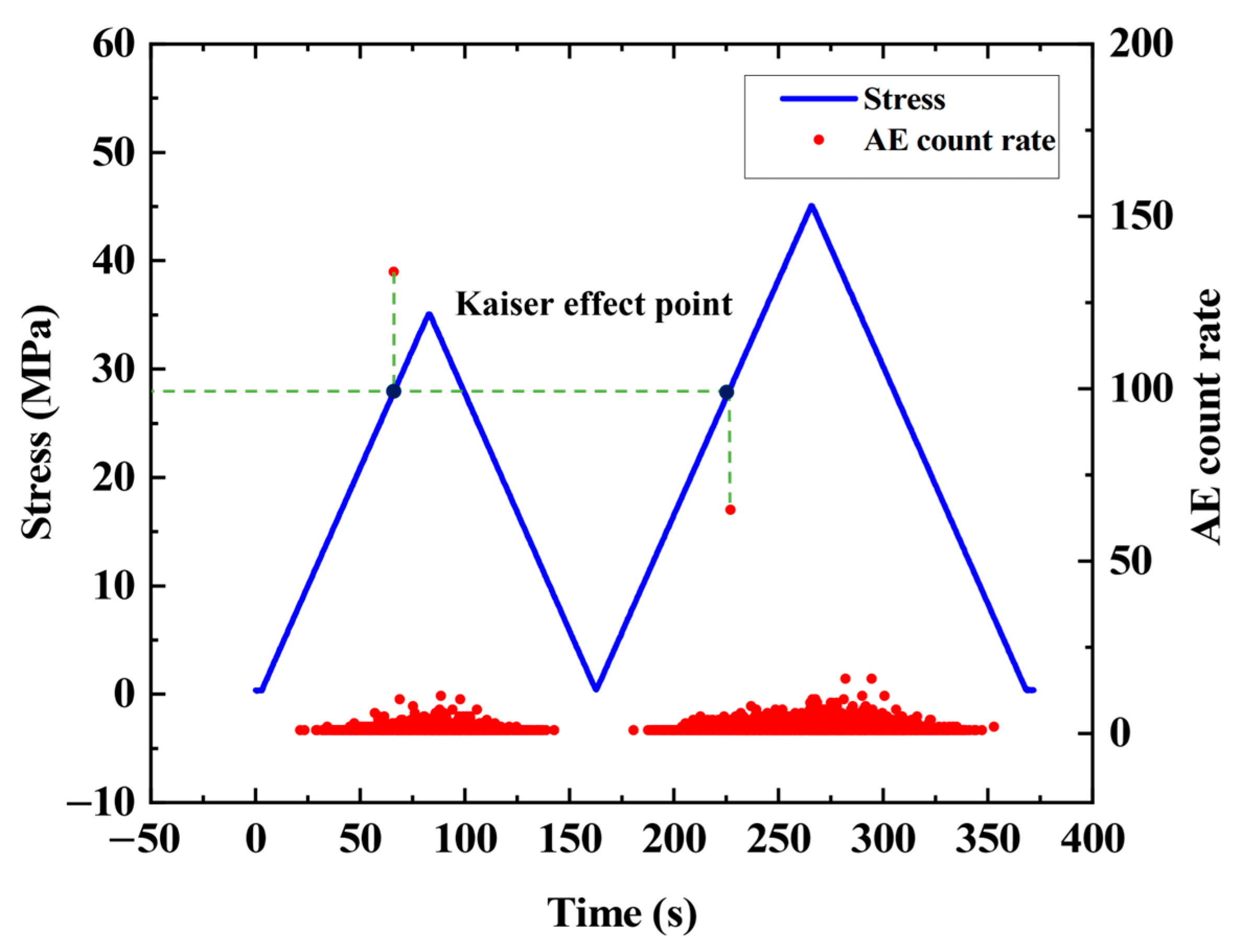
To more accurately investigate the distribution patterns of the in situ stress field in the deep mining area of a certain mine, this study conducted supplementary tests focusing on depths between −250 m and −300 m, based on previous in situ stress measurement results obtained via the stress relief method at the −215 m level (numbered 1). Given the complex geological environment of deep mines, high in situ stress leads to severe borehole deformation and core fracturing, which renders traditional methods such as the hydraulic fracturing method or the overcoring stress relief method difficult to implement in deep zones and results in low drilling success rates. Therefore, the acoustic emission (AE) method was adopted for in situ stress measurement in this study. This method is based on the Kaiser effect of rocks, namely the characteristic that rocks have a “memory” of their stress history: when a rock specimen is loaded beyond the maximum stress level it has previously experienced, acoustic emission signals increase significantly. By monitoring the characteristic point of the Kaiser effect through laboratory uniaxial compression tests, the in situ normal stress in this direction can be determined. Although the AE method provides a feasible stress measurement scheme for deep regions, its limitations and potential uncertainties must be acknowledged. First, the identification of Kaiser effect points relies on the memory of the historical maximum stress, which can be affected by the degree of rock damage and time delay. Therefore, we preferentially selected intact core samples to avoid the influence of pre-existing microcracks on signal quality.

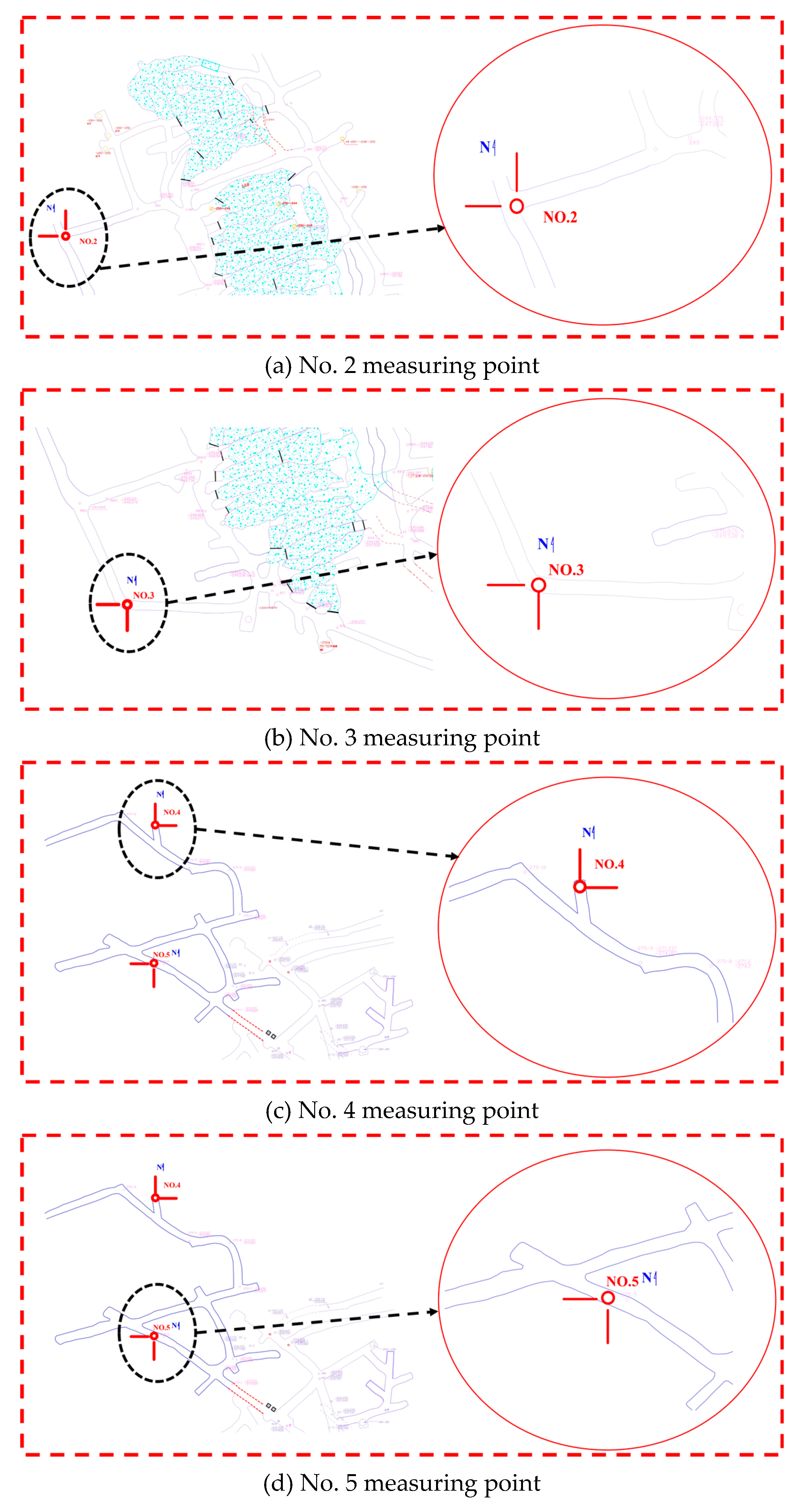
To ensure the reliability and representativeness of the test data, the layout of measuring points followed the following principles: (1) areas with faults, fractured zones, or abrupt lithological changes should be avoided; instead, homogeneous and intact rock masses were selected to ensure high-quality core sampling; (2) roadway excavation disturbance zones and stress concentration distortion zones should be avoided to ensure that the measured data reflect the in situ rock stress state. Based on the above principles, the on-site sampling of this study was mainly carried out at two key levels of −250 m and −275 m, with a total of four measuring points (numbered 2, 3, 4, 5) arranged in the drift outside the ore vein. To obtain the in situ stress state of each measuring point, borehole coring was performed along two horizontal directions (or their opposite directions) of 0° and 90° at each measuring point, with the true north direction set as the 0° reference. The sampling position and drilling direction of acoustic emission in situ stress test are shown in Figure 2.

The PCI-2 acoustic emission testing system was utilized for acoustic emission (AE) signal acquisition in laboratory experiments. During the experiment, the load variation and AE signals of rock specimens under uniaxial compression were monitored and collected synchronously, with AE count rate and amplitude selected as the key characteristic parameters to identify the Kaiser effect points. Based on the stress values corresponding to the Kaiser effect points of rock cores sampled in different directions, the magnitude and direction of the principal stress at each measuring point were obtained through calculation. Given that AE signals are susceptible to environmental noise, a rigorous manual inspection method was adopted to ensure data reliability. Instead of automated statistical filtering, we relied on expert experience to identify the Kaiser effect points by analyzing the slope changes in the cumulative AE count curve. Any ambiguous signals or data points that did not exhibit clear Kaiser effect characteristics were discarded from the dataset to ensure the physical validity of the training samples. The acoustic emission signal test diagrams of rock specimens and the in situ stress measurement results are presented in Figure 3 and

Table 1. Actual measurement of in situ stress.

Test No.	Level (m)	Depth (m)	${\mathit{\sigma }}_{\mathit{x}}$(MPa)	${\mathit{\sigma }}_{\mathit{y}}$(MPa)	${\mathit{\sigma }}_{\mathit{z}}$(MPa)
1	−215	990	21.23	30.61	20.22
2	−250	1025	24.61	29.39	22.31
3	−250	1025	24.91	29.21	22.46
4	−275	1050	24.64	31.27	24.06
5	−275	1050	25.13	31.87	24.52

, respectively.

4. In Situ Stress Field Inversion Model Construction

4.1. 3D Numerical Model Establishment

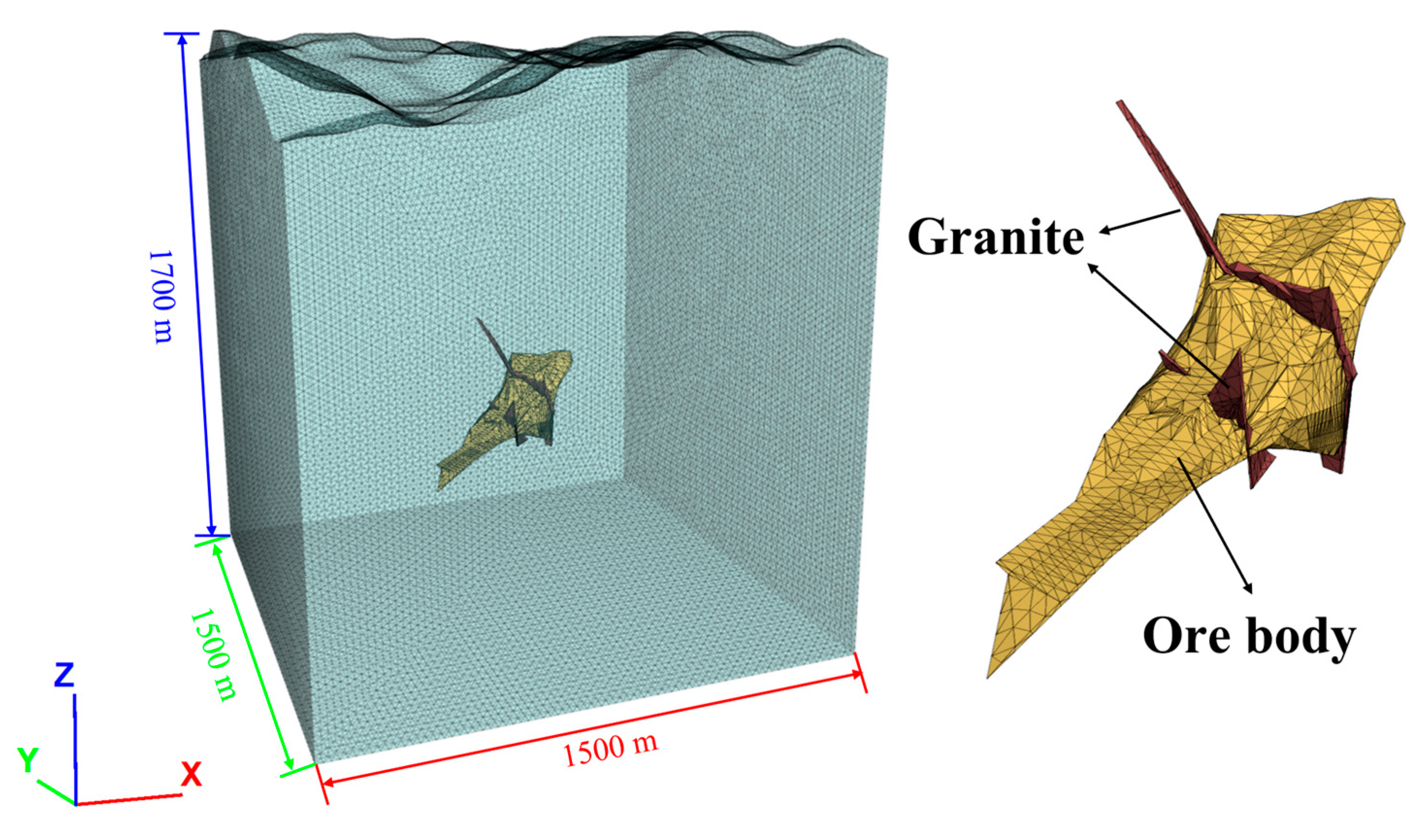
FLAC^3D was employed as the numerical simulation platform. Combined with the topography, geomorphology, and geological structure of the mining area, a three-dimensional geological model of the deep ore body and surrounding rock was established using MIDAS and 3DMine software, with model dimensions of 1500 m × 1500 m × 1700 m. To improve the calculation accuracy, the meshes of the mining area and in situ stress measurement points were further refined, with a minimum mesh density of 1 m. The overall model consists of 502,166 nodes and 2,883,282 elements. Although deep rock masses exhibit anisotropy, it is extremely difficult to obtain accurate large-scale anisotropic parameters. The use of poorly constrained parameters would introduce additional errors into the numerical results. Moreover, as disturbances induced by underground roadway excavation and mining operations are not considered in this study, an isotropic elastic constitutive model is employed. The established three-dimensional geological model is shown in Figure 4, and the physical and mechanical parameters of the rock mass are listed in

Table 2. Mechanical parameters of rock mass.

Rock Type	Volume Modulus (GPa)	Shear Modulus (GPa)	Density (g/cm3)	Cohesion (MPa)	Internal Friction Angle (°)	Tensile Strength (MPa)	Poisson’s Ratio
Surrounding rock	17.93	10.76	2.70	4.03	42.05	0.63	0.31
Ore	21.26	13.38	4.40	4.65	43.34	0.93	0.24
Granite	26.58	16.51	2.62	8.41	48.59	2.72	0.10

. These parameters were derived from laboratory tests on intact rock specimens and subsequently adjusted using the Hoek–Brown strength criterion and the Geological Strength Index (GSI) based on field geological surveys. This reduction method ensures that the numerical model accurately reflects the mechanical behavior of the fractured rock mass in the deep mining area.

4.2. Model Boundary Conditions and Training Sample Construction

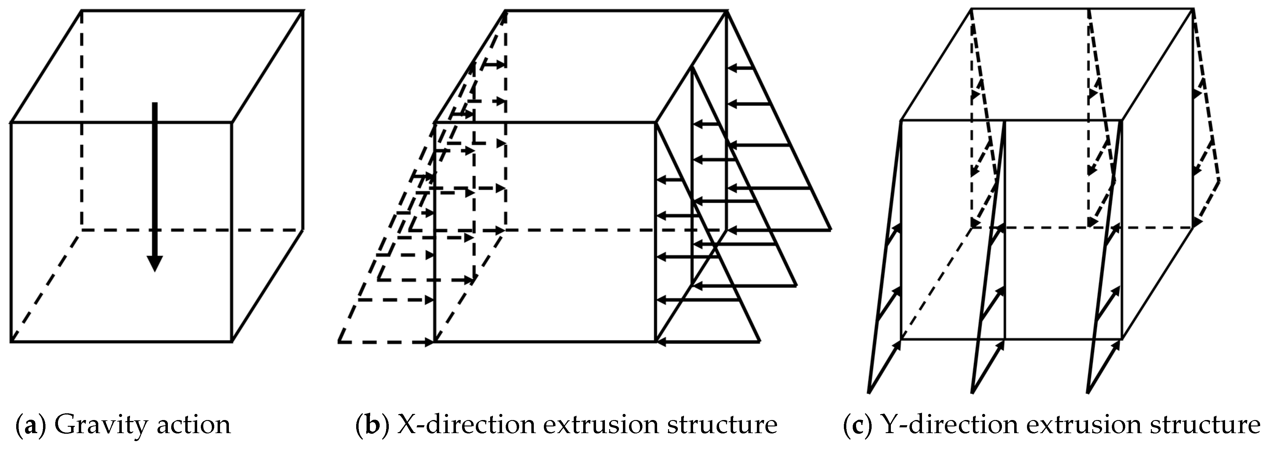
Deep in situ stress fields are mainly formed by superposition of the self-weight stress field and the tectonic stress field of the surrounding rock. Different combinations of boundary condition loads were set in the FLAC^3D numerical simulation to simulate historical tectonic movements. The main influencing factors considered in the in situ stress field inversion research of this paper include: (1) gravitational stress; (2) horizontal tectonic compression in the x-direction; and (3) horizontal tectonic compression in the y-direction. The schematic diagram of boundary condition loads is shown in Figure 5.

Considering the inhomogeneity and depth gradient effect of deep horizontal tectonic stress, horizontally graded stresses were applied to the x-direction and y-direction side boundaries of the model, respectively. According to the results of previous in situ stress measurements in the mine, the relational equations between the deep horizontal principal stresses and the burial depth are expressed as follows:

$$\left\{\begin{array}{l}{\sigma }_x=0.017\cdot H+2.77 (\mathrm{MPa})\hfill \\ {\sigma }_y=0.040\cdot H-0.55 (\mathrm{MPa})\hfill \end{array}\right.$$

(9)

To meet the training requirements of the model, an orthogonal experimental design was adopted to construct the training sample set for the ABC-SVR intelligent inversion algorithm model. A total of 40 sets of boundary conditions were established based on the gravity correction coefficient $K_v$, x-direction gradient stress correction coefficient $K_x$ and y-direction gradient stress correction coefficient $K_y$. The gravity correction coefficient was set within a range of ±20%, while the x-direction and y-direction gradient stress correction coefficients were set within a range of ±30%. The parameters of each set of boundary conditions are listed in

Table 3. Orthogonal design table.

Number	${\mathit{K}}_{\mathit{v}}$	${\mathit{K}}_{\mathit{x}}$	${\mathit{K}}_{\mathit{y}}$
1	1.09	1.22	1.19
2	0.87	0.92	1.20
3	1.05	1.00	1.12
4	0.96	1.05	1.15
5	0.89	1.24	0.76
6	1.20	1.12	0.80
7	1.02	0.90	0.86
8	1.03	0.97	1.30
9	1.06	1.27	0.87
10	1.10	0.83	1.23
11	0.95	1.07	0.83
12	1.07	0.89	1.04
13	0.84	0.84	0.73
14	0.88	1.20	0.91
15	0.94	0.73	0.78
16	0.98	0.82	0.96
17	1.13	1.09	1.07
18	0.99	1.30	1.10
19	0.82	1.26	1.05
20	1.14	1.02	0.99
21	0.86	0.72	1.01
22	1.19	0.93	0.95
23	0.98	1.14	0.90
24	1.09	1.04	0.74
25	1.15	0.87	0.75
26	1.12	1.19	1.02
27	1.03	1.18	0.70
28	0.82	1.10	1.28
29	0.84	1.12	0.97
30	1.05	0.70	0.93
31	0.92	1.15	1.22
32	0.94	0.98	1.18
33	0.80	0.95	0.82
34	1.17	1.24	1.24
35	0.88	0.86	1.12
36	0.91	0.78	1.08
37	1.00	0.75	1.26
38	1.18	0.80	1.16
39	0.91	1.00	0.89
40	1.11	0.77	0.85

.

4.3. Data Normalization Processing

Based on the numerical simulation scheme designed via orthogonal experiment, a program was written in FISH language within FLAC^3D to extract the calculated stress values at the coordinates of measured points corresponding to each set of boundary conditions in the calculation model. A sample library was established where boundary conditions were set as the input values of the model, and the corresponding stress values at measured points were set as the output values. Since there are significant differences in the dimensions of input and output parameters designed in the dataset, directly using raw data tends to reduce the generalization ability of the model and the optimization convergence speed of the ABC algorithm. To eliminate the influence of dimensions, the data need to be standardized as a preprocessing step. This study adopted the min-max normalization method, which linearly maps the input and output parameters to a dimensionless interval of [0, 1]. Its calculation formula is expressed as follows:

$$x^{\prime }={\displaystyle \frac{x-x_{\min }}{x_{\max }-x_{\min }}}$$

(10)

where $\mathrm{x}$ and ${\mathrm{x}}^{\prime }$ are the variable values before and after normalization, respectively; and ${\mathrm{x}}_{\max }$ and ${\mathrm{x}}_{\min }$ are the maximum and minimum values in the sample library before normalization, respectively.

After the model training and prediction were completed, the normalized output data were inversely normalized back to the original physical scale (MPa).

5. In Situ Stress Inversion Analysis

5.1. Model Training Parameter Setting

The establishment of the ABC-SVR model requires the setting of relevant parameters, such as population size and number of iterations. Based on simulation analysis of the experimental data, the ABC algorithm was used to optimize the penalty parameter C and kernel function parameter γ. The population size of the ABC algorithm was set to 30 based on a preliminary sensitivity analysis. Tests with population sizes ranging from 10 to 50 indicated that a size of 30 offered the best trade-off between convergence speed and solution diversity. Increasing the population beyond 30 did not significantly improve the MSE but increased the computational cost, the maximum number of iterations to 100, and the limit value to 50. The search space boundaries of the SVR algorithm were set as follows: penalty factor C: [1, 1000], kernel parameter γ: [0.1, 100].

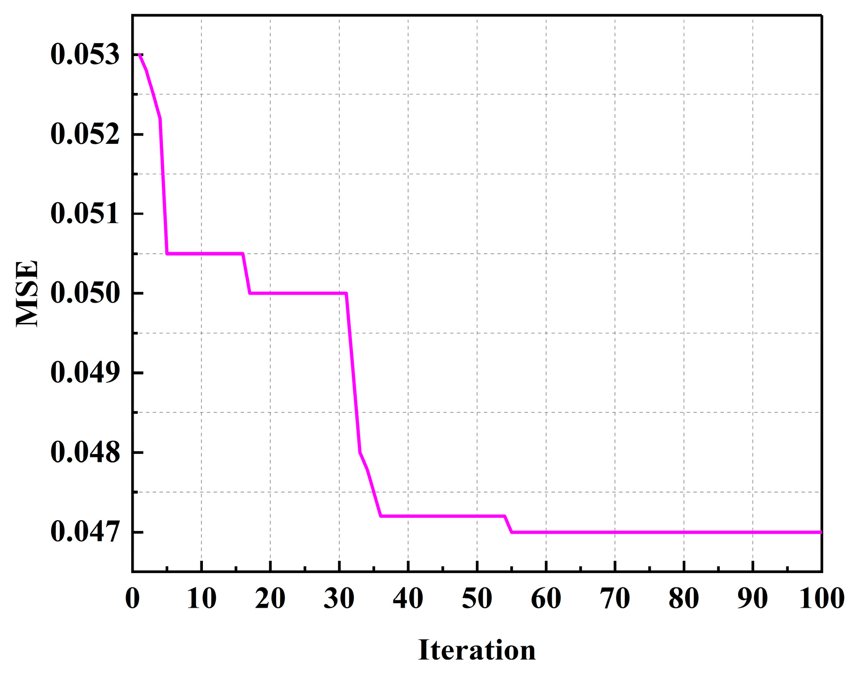
The mean squared error (MSE) of the training set with five-fold cross-validation was used as the fitness function. It should be noted that five-fold cross-validation was strictly used for hyperparameter tuning (i.e., identifying the optimal penalty factor C and kernel parameter γ) rather than for model averaging. Once the optimal parameter combination was determined via the cross-validation process, the final ABC-SVR model was retrained on the entire training set to maximize information utilization and prediction performance, and Figure 6 shows the fitness convergence curve of the ABC algorithm during the parameter optimization process. As can be seen from the figure, the MSE of the model decreased rapidly at the initial stage of iteration, indicating that the model quickly found a relatively good solution region in the early training stage. A plateau period appeared subsequently, which means the algorithm was trapped in a local optimum and was searching for a better solution in the surrounding area through “onlooker bees” or “scout bees”. Following this, the curve dropped sharply again, demonstrating that the algorithm found a better combination of parameters. When the number of iterations reached 55, the curve became stable and finally achieved steady convergence, with the MSE stabilizing at approximately 0.047. This indicates that the ABC algorithm is a feasible parameter optimization algorithm that can prevent the SVR algorithm from falling into local optima. The optimal parameters of the ABC-SVR model were finally determined as C = 124.56, γ = 0.48.

5.2. Boundary Condition Inversion Result Analysis

5.2.1. Inversion Result Analysis

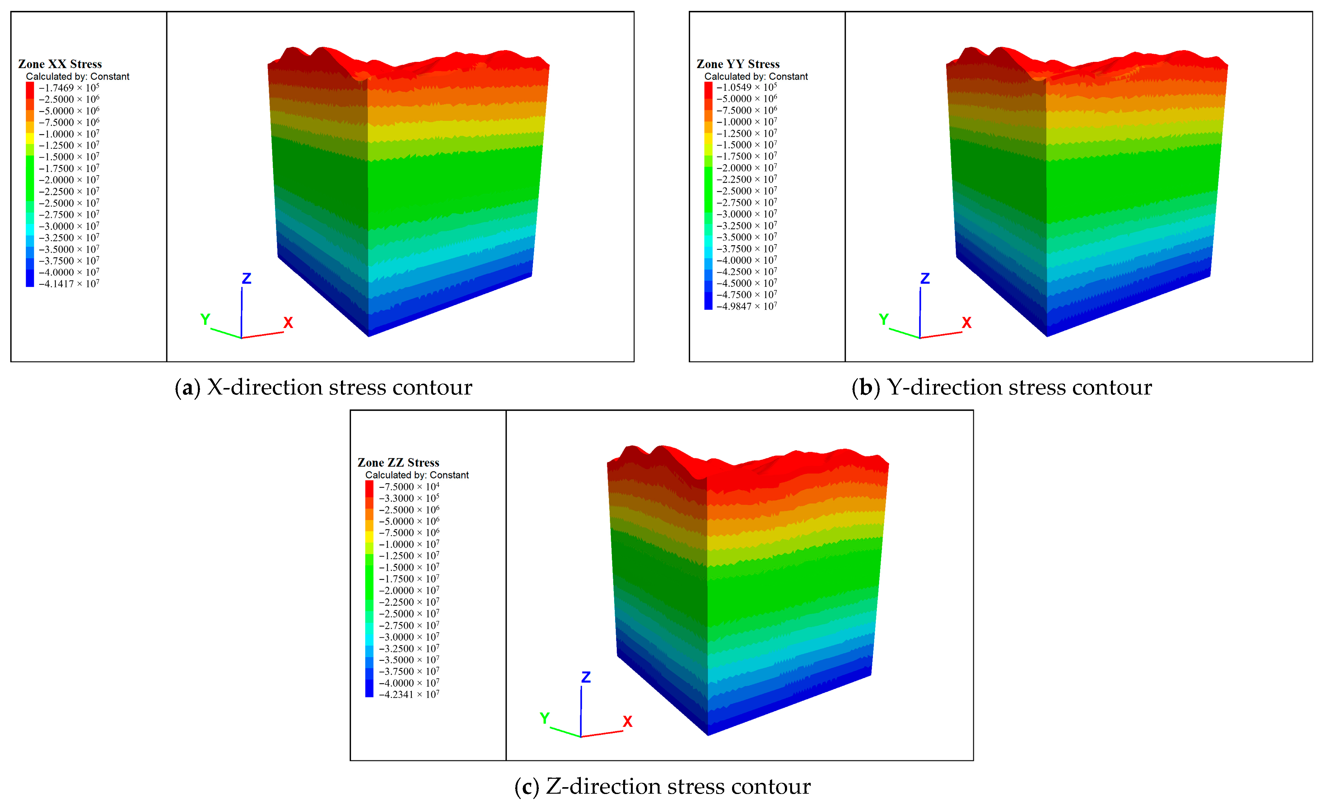
To verify the inversion advantages of the ABC-SVR inversion model in deep areas with few samples, a comparative experiment was conducted among this model, grid search-based SVR [40], and a standard BP neural network. Inversion calculations were performed using the in situ stress data for five measured points. The optimal boundary load correction coefficients obtained using each algorithm are listed in

Table 4. Inversion results of boundary condition parameters.

Model	${\mathit{K}}_{\mathit{v}}$	${\mathit{K}}_{\mathit{x}}$	${\mathit{K}}_{\mathit{y}}$
ABC-SVR	1.02	1.18	0.86
SVR	1.05	1.09	0.95
BP	1.08	1.26	0.78

. To evaluate the effectiveness of the inverted boundary conditions, the boundary condition parameters obtained via inversion were converted into boundary loads, which were then imported into the FLAC^3D calculation model. The overall stress field was derived through model inversion, and the 3D contour maps of principal stresses are shown in Figure 7.

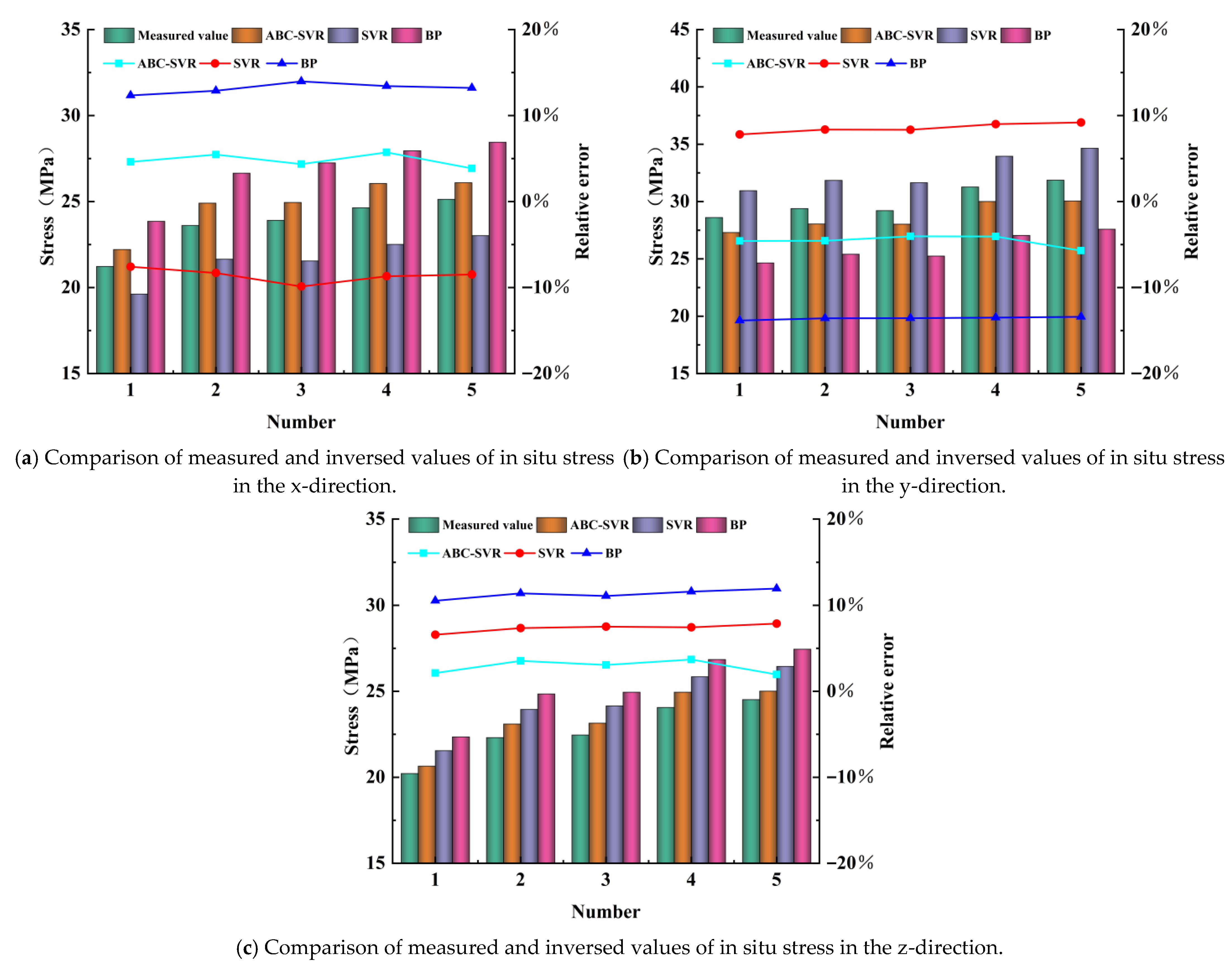
The inverted stress values of five measuring points were extracted, and a comparison of the measured values and the inverted stress values predicted by the three algorithms are presented in

Table 5. Comparison of inversion values and measured values.

Test No.	Method	X-Direction Stress		Y-Direction Stress		Z-Direction Stress
		${\mathit{\sigma }}_{\mathbf{x}}$ (MPa)	Relative Error (%)	${\mathit{\sigma }}_{\mathbf{y}}$ (MPa)	Relative Error (%)	${\mathit{\sigma }}_{\mathbf{z}}$ (MPa)	Relative Error (%)
1	Measured	21.23	0	28.61	0	20.22	0
	ABC-SVR	22.21	4.62	27.30	−4.58	20.65	2.13
	SVR	19.62	−7.58	30.95	8.18	21.55	6.58
	BP	23.85	12.34	24.65	−13.84	22.35	10.53
2	Measured	23.61	0	29.39	0	22.31	0
	ABC-SVR	24.91	5.46	28.05	−4.56	23.10	3.54
	SVR	21.65	−8.30	31.85	8.37	23.95	7.35
	BP	26.65	12.88	25.41	−13.58	24.85	11.39
3	Measured	23.91	0	29.21	0	22.46	0
	ABC-SVR	24.95	4.35	28.03	−4.04	23.15	3.07
	SVR	21.55	−9.87	31.65	8.35	24.15	7.52
	BP	27.25	13.97	25.25	−13.56	24.95	11.09
4	Measured	24.64	0	31.27	0	24.04	0
	ABC-SVR	26.05	5.72	30.01	−4.06	24.95	3.70
	SVR	22.51	−8.69	33.95	8.57	25.85	7.44
	BP	27.95	13.43	27.05	−13.49	26.85	11.59
5	Measured	25.13	0	31.87	0	24.52	0
	ABC-SVR	26.10	3.86	30.05	−5.71	25.01	1.96
	SVR	23.02	−8.48	34.65	8.72	26.45	7.87
	BP	28.45	13.21	27.59	−13.40	27.45	11.95

and Figure 8.

From a macroscopic perspective, the measured in situ stress data indicate that the deep in situ stress field of this mining area exhibits a depth-gradient distribution pattern; namely, all three principal stress components show a tendency to increase with increasing depth. By comparing the inversion results, it can be found that all three algorithms have captured this pattern, which demonstrates that, after training with the same training samples, the selected machine learning models can all correctly learn the correlation mechanism between boundary loads and deep in situ stresses.

Although the inversion trends are consistent, the inversion accuracy of different algorithms varies significantly. As can be seen from Table 5, both the ABC-SVR and SVR algorithms achieve favorable performance in in situ stress inversion. The relative error between the in situ stress results inverted by the ABC-SVR algorithm and the measured values ranges from 1.96% to 5.72%, with an average relative error of 4.16%, indicating optimal inversion performance. The relative error between the measured point stress values inverted by the traditional SVR algorithm and the measured values ranges from 6.58% to 9.87%, with an average relative error of 8.12%, ranking second in terms of performance. The inversion results of the BP neural network are the worst; the relative error between the inverted measured point stress values and the measured values ranges from 10.53% to 13.84%, with an average relative error of 12.71%. This indicates that the BP neural network is prone to falling into local optimal solutions under small-sample conditions, resulting in overfitting and underfitting of the algorithm model in nonlinear mapping. In contrast, the SVR optimized by ABC significantly improves the inversion prediction accuracy compared with the traditional SVR and BP neural network and can exhibit stronger generalization ability under small-sample conditions.

It is worth noting that a comparison of the error results of each component reveals that the inversion errors of the three algorithm models for the vertical stress component are all lower than those for the horizontal principal stresses. Taking the ABC-SVR algorithm with the lowest average relative error as an example, its error for the vertical stress component is only in the range of 1.96% to 3.70%. The reason for this phenomenon is that the vertical stress of the deep rock mass is mainly dominated by the self-weight of the overlying strata, and its magnitude has a relatively strict linear relationship with depth. Therefore, both SVR and BP neural networks can converge rapidly during the training process of learning this mapping relationship and achieve relatively high fitting accuracy. In contrast, the genesis of horizontal principal stress is more complex; it is not only affected by the lateral pressure induced by rock mass self-weight, but also by multiple factors such as geological tectonic movements and rock mass anisotropy, often exhibiting high nonlinearity and discreteness with changes in depth. However, the established three-dimensional numerical model has simplified the stratum and geological structures, thus increasing the difficulty for the inversion model to find the optimal solution. Among the three models, the ABC-SVR algorithm can still maintain a small inversion error in the inversion of horizontal principal stress, which further proves its advantages in dealing with strong nonlinear mapping problems.

5.2.2. Model Performance Evaluation

To quantitatively evaluate the effectiveness and reliability of different intelligent algorithms in the inversion of deep and complex in-situ stress fields, three performance metrics, namely the mean absolute percentage error (MAPE), root mean square error (RMSE), and coefficient of determination (R²), were selected in this study for a comprehensive evaluation of the inversion performance of each algorithm model. Their mathematical expressions are given as follows:

$$\mathrm{MAPE}={\displaystyle \frac{1}{n}}{\displaystyle \sum _{i=1}^n\left|\frac{y_i-y_p}{y_i}\right|}$$

(11)

$$\mathrm{RMSE}=\sqrt{{\displaystyle \frac{1}{n}}\times {\displaystyle \sum _{i=1}^n{(y_i-y_p)}^2}}$$

(12)

$${\mathrm{R}}^2={\displaystyle \frac{{\displaystyle \sum _{i=1}^n{(y_i-y_{\mathrm{mean}})}^2}-{\displaystyle \sum _{i=1}^n{(y_i-y_p)}^2}}{{\displaystyle \sum _{i=1}^n{(y_i-y_{\mathrm{mean}})}^2}}}$$

(13)

where $n$ is the number of samples of the measured in situ stress values, and $y_i$, $y_p$, and $y_{mean}$ are the measured value, inverted value, and average value of in situ stress, respectively.

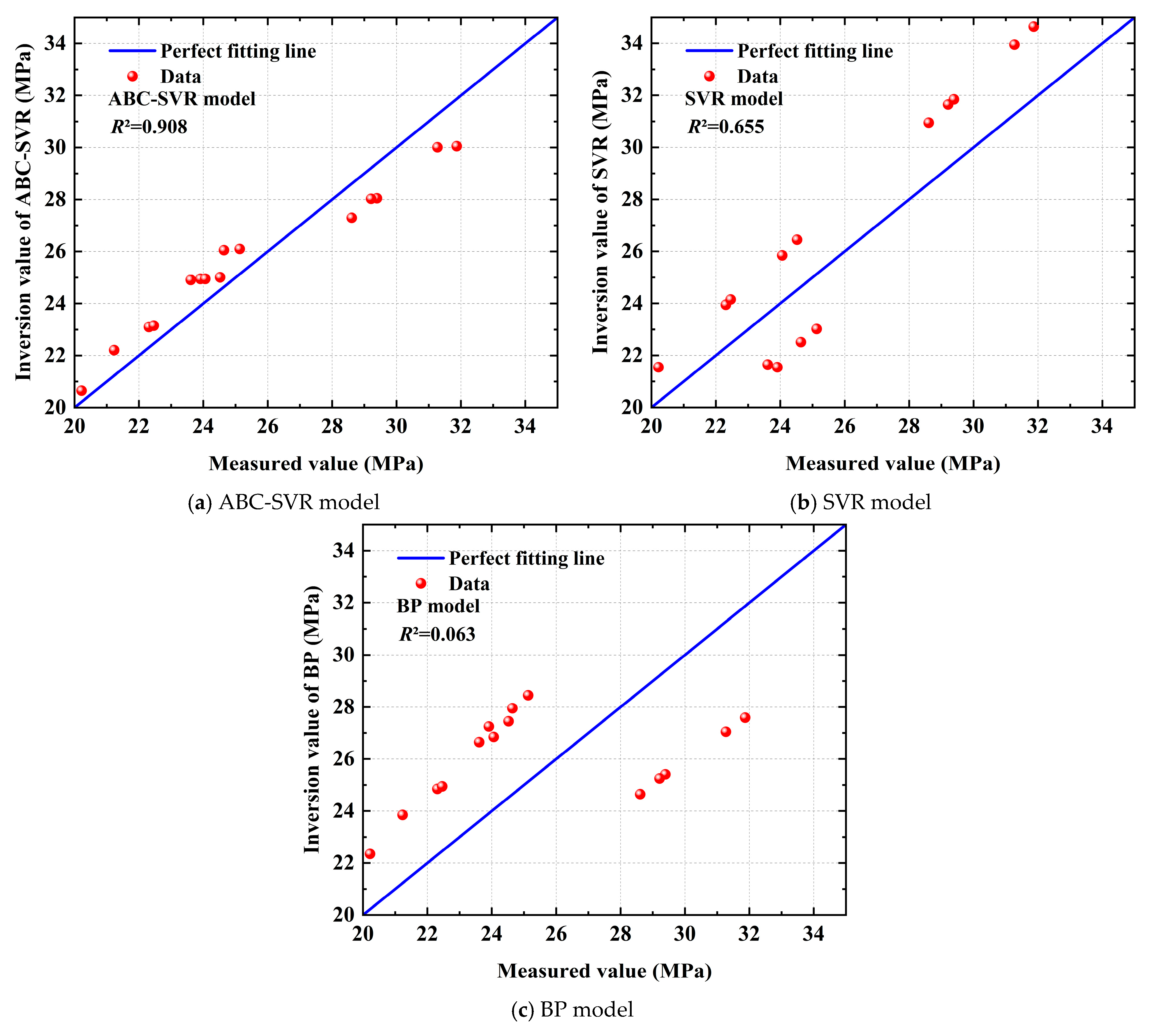
The inversion performance of the three intelligent algorithm models is presented in

Table 6. Performance comparison of the three different models.

Evaluation Indicator	ABC-SVR	SVR	BP
R2	0.908	0.655	0.063
RMSE	1.25	2.31	3.58
MAPE	4.16	8.12	12.71

. The mean absolute percentage error (MAPE) reflects the deviation degree of the model inversion values relative to the measured values, directly embodying the engineering reliability of the inversion results. The MAPE of ABC-SVR is 4.16%, which is superior to that of SVR (8.12%) and BP (12.71%). The root mean square error (RMSE) is commonly used to measure the robustness of the model; the RMSE of ABC-SVR is 1.25, which is significantly lower than that of SVR (2.31) and BP (3.58). Figure 9 shows the correlation between the inversion results and measured values of the ABC-SVR, SVR, and BP models. Due to the small depth span of each measuring point, the measured in situ stress values do not change significantly, and there is no large magnitude jump, resulting in a small total variance of the data itself. The R² index exhibits extremely high sensitivity to prediction residuals. Although the relative errors of the comparative algorithms SVR and BP neural network are within a certain range (8.12% and 12.71%), their failure to capture minor fluctuations in the data leads to extremely small values of the coefficient of determination R². In contrast, the ABC-SVR still achieves excellent performance with R² = 0.908 under the harsh conditions of small total variance of measured data and strong nonlinearity, which fully demonstrates the model’s excellent ability to sensitively capture minor stress changes.

Combined with the performance evaluation results of R², RMSE, and MAPE, the ABC-SVR model exhibits excellent performance in the in situ stress inversion measurement of deep mining areas with few samples, and is thus a high-precision inversion method for deep complex geological environments.

6. Discussion

Due to the limited number of measured samples and the fact that the in situ stress field is affected by multiple factors such as geological tectonic movements and surrounding rock conditions, certain errors still exist in the inversion prediction results. The training samples required for in situ stress field inversion using machine-learning algorithms are derived from numerical simulation calculations, while the established 3D numerical model has simplified the strata and geological structures. Therefore, constructing a more refined 3D numerical model that conforms to actual geological structural conditions to obtain more realistic training samples is a key step to improve inversion accuracy, and it is also a research focus for in situ stress field inversion in the future.

7. Conclusions

To address the challenges of high inversion difficulty caused by limited measured in situ stress samples and complex tectonic stress in deep mining areas, this study proposes an in situ stress field inversion model based on support vector regression optimized by the artificial bee colony algorithm. Combining the ABC-SVR intelligent inversion algorithm with the 3D numerical simulation method, the intelligent inversion of the initial in situ stress field in the deep mining area of a mine was successfully realized. Through comparative studies with the traditional SVR and BP neural network algorithms, as well as verification using measured in situ stress data, the main conclusions are drawn as follows:

(1)

To address the issues of severe deformation and low drilling success rate in high-stress deep zones, an acoustic emission method based on the Kaiser effect was successfully employed to measure in situ stress at monitoring points. By adhering to strict sampling principles and conducting manual Kaiser effect point verification, reliable in situ stress data were obtained, providing a solid physical foundation for subsequent stress field inversion.

(2)

The inversion results show that the predicted values of in situ stress obtained by the ABC-SVR algorithm are in good agreement with the measured in situ stress results. The model achieves an RMSE of 1.25, a coefficient of determination R² of 0.908, and a mean absolute percentage error (MAPE) of 4.16%. All performance metrics are significantly superior to those of the traditional SVR and BP neural network algorithms, demonstrating the high-precision advantage of this method for deep in situ stress inversion.

(3)

For in situ stress inversion measurement of deep mining areas, the artificial bee colony algorithm can realize parameter optimization of the SVR model, improve its generalization ability, and avoid falling into local optimal solutions. The inversion results can provide reliable initial in situ stress field data support for mining design and deep mine roadway support, and thus have significant practical engineering value.

References

1. Deng, R.Q.; Zhang, Y.; Wu, D.; Lv, J.K.; Jing, Y.N.; Zhen, Z.; Shi, P. Inversion of In-situ stress field in near-fault coal mining area by coupling numerical simulation with deep learning. Geomat. Nat. Hazards Risk 2025, 16, 13. [Google Scholar] [CrossRef]
2. Hao, Y.; Liu, C.H.; Wu, Y.; Pu, H.; Zhang, K.; Shen, L.L. Analysis of Stress and Deformation on Surrounding Rock Mass of a Trapezoidal Roadway in a Large Inclination Coal Seam and Novel High Yielding Prop Support: A Case Study. Mathematics 2023, 11, 319. [Google Scholar] [CrossRef]
3. Zhao, Y.; Zhao, G.Y.; Zhou, J.; Cai, X.; Ma, J. Mining Stress Evolution Law of Inclined Backfilled Stopes Considering the Brittle-Ductile Transition in Deep Mining. Mathematics 2022, 10, 1308. [Google Scholar] [CrossRef]
4. Li, P.; Cai, M.F. Challenges and new insights for exploitation of deep underground metal mineral resources. Trans. Nonferrous Met. Soc. China 2021, 31, 3478–3505. [Google Scholar] [CrossRef]
5. Liu, X.F.; Wang, E.Y. Study on characteristics of EMR signals induced from fracture of rock samples and their application in rockburst prediction in copper mine. J. Geophys. Eng. 2018, 15, 909–920. [Google Scholar] [CrossRef]
6. Ranjith, P.G.; Zhao, J.; Ju, M.H.; De Silva, R.V.S.; Rathnaweera, T.D.; Bandara, A. Opportunities and Challenges in Deep Mining: A Brief Review. Engineering 2017, 3, 546–551. [Google Scholar] [CrossRef]
7. Fairhurst, C. Some Challenges of Deep Mining. Engineering 2017, 3, 527–537. [Google Scholar] [CrossRef]
8. Zhang, W.; Zhang, Y.D.; Zhu, Y.C.; Tang, J.J.; Cheng, L.T.; Suo, Z.L. Integrated Collaborative Control of “Shielding-Filling-Grouting” of 1 km Deep Large-Section Roadways: A Case Study. Minerals 2022, 12, 854. [Google Scholar] [CrossRef]
9. Li, P.; Cai, M.F.; Miao, S.J.; Ren, F.H.; Gorjian, M.; Peng, C. Mechanism, prevention, and control of mining-induced dynamic disasters in underground metal mines in China: Challenges and solutions. J. Cent. South Univ. 2024, 31, 2549–2606. [Google Scholar] [CrossRef]
10. Shi, K.Y.; Liu, Y.; Liang, W.Z. An Extended ORESTE Approach for Evaluating Rockburst Risk under Uncertain Environments. Mathematics 2022, 10, 1699. [Google Scholar] [CrossRef]
11. Liu, Z.; Chen, J.H.; Zhao, Y.K.; Yang, S. A Novel Method for Predicting Rockburst Intensity Based on an Improved Unascertained Measurement and an Improved Game Theory. Mathematics 2023, 11, 1862. [Google Scholar] [CrossRef]
12. Bondarenko, V.; Kovalevska, I.; Krasnyk, V.; Chernyak, V.; Haidai, O.; Sachko, R.; Vivcharenko, I. Methodical principles of experimental-analytical research into the influence of pre-drilled wells on the intensity of gas-dynamic phenomena manifestations. Min. Miner. Deposits 2024, 18, 67–81. [Google Scholar] [CrossRef]
13. Symanovych, H.; Lisovytska, I.; Odnovol, M.; Ahaiev, R.; Poimanov, S. Rationale and modeling of technology for complex bottom-hole zone de-stressing of gas-dynamically active rock mass. Min. Miner. Deposits 2024, 18, 83–92. [Google Scholar] [CrossRef]
14. Zhao, X.G.; Wang, J.; Cai, M.; Ma, L.K.; Zong, Z.H.; Wang, X.Y.; Su, R.; Chen, W.M.; Zhao, H.G.; Chen, Q.C.; et al. In-situ stress measurements and regional stress field assessment of the Beishan area, China. Eng. Geol. 2013, 163, 26–40. [Google Scholar] [CrossRef]
15. Shi, X.C.; Zhang, J.X.; Li, G.Q. Characteristics of in situ stress field in the Huainan mining area, China and its control factors. Environ. Earth Sci. 2021, 80, 18. [Google Scholar] [CrossRef]
16. Jing, W.; Zhou, J.; Yuan, L.; Jin, R.C.; Jing, L.W. Deformation and Failure Mechanism of Surrounding Rock in Deep Soft Rock Tunnels Considering Rock Rheology and Different Strength Criteria. Rock Mech. Rock Eng. 2024, 57, 545–580. [Google Scholar] [CrossRef]
17. Liu, B.; Zhu, Y.G.; Liu, Q.S.; Liu, X.W. A Novel in Situ Stress Monitoring Technique for Fracture Rock Mass and Its Application in Deep Coal Mines. Appl. Sci. 2019, 9, 3742. [Google Scholar] [CrossRef]
18. Ma, C.D.; Tan, G.S.; Li, X.B.; Xu, J.Q.; Chen, J.Z. Core Orientation Technology Based on Drilling Trajectory Projection and Its Application in In Situ Stress Measurement of the Deepest Shaft in China. Minerals 2022, 12, 521. [Google Scholar] [CrossRef]
19. Bao, T.; Burghardt, J. A Bayesian Approach for In-Situ Stress Prediction and Uncertainty Quantification for Subsurface Engineering. Rock Mech. Rock Eng. 2022, 55, 4531–4548. [Google Scholar] [CrossRef]
20. Han, Z.Q.; Wang, C.Y.; Wang, Y.T.; Wang, C. Borehole Cross-Sectional Shape Analysis under in Situ Stress. Int. J. Geomech. 2020, 20, 6. [Google Scholar] [CrossRef]
21. Yan, H.C.; Liu, H.Z.; Li, Y.; Zhuo, L.; Xiao, M.L.; Chen, K.P.; Wu, J.M.; Pei, J.L. Inversion Analysis of the In Situ Stress Field around Underground Caverns Based on Particle Swarm Optimization Optimized Back Propagation Neural Network. Appl. Sci. 2023, 13, 4697. [Google Scholar] [CrossRef]
22. Yu, R.S.; Tan, Z.S.; Gao, J.P.; Wang, X.Y.; Zhao, J.P. Inversion and Analysis of the Initial Ground Stress Field of the Deep-Buried Tunnel Area. Appl. Sci. 2022, 12, 8986. [Google Scholar] [CrossRef]
23. Zhang, Z.Q.; Gong, R.K.; Zhang, H.; Lan, Q.N.; Tang, X. Initial ground stress field regression analysis and application in an extra-long tunnel in the western mountainous area of China. Bull. Eng. Geol. Environ. 2021, 80, 4603–4619. [Google Scholar] [CrossRef]
24. Liang, J.; Zhu, Q.J.; Sui, L.K.; Duan, L.; Wang, D.C. Research on Elaborate Construction of Complex 3D Geological Model and In-Situ Stress Inversion. Geotech. Geol. Eng. 2024, 42, 1373–1388. [Google Scholar] [CrossRef]
25. Chen, B.; Ren, Q.Y.; Wang, F.F.; Zhao, Y.C.; Liu, C.D. Inversion Analysis of In-Situ Stress Field in Tunnel Fault Zone Considering High Geothermal. Geotech. Geol. Eng. 2021, 39, 5007–5019. [Google Scholar] [CrossRef]
26. Li, Y.; Guo, Y.H.; Zhu, W.S.; Li, S.C.; Zhou, H. A modified initial in-situ Stress Inversion Method based on FLAC3D with an engineering application. Open Geosci. 2015, 7, 824–835. [Google Scholar] [CrossRef]
27. Zhang, J.G.; Li, P.T.; Yin, X.; Wang, S.; Zhu, Y.G. Back Analysis of Surrounding Rock Parameters in Pingdingshan Mine Based on BP Neural Network Integrated Mind Evolutionary Algorithm. Mathematics 2022, 10, 1746. [Google Scholar] [CrossRef]
28. Li, J.H.; Sun, W.Z.; Su, G.S.; Zhang, Y. An Intelligent Optimization Back-Analysis Method for Geomechanical Parameters in Underground Engineering. Appl. Sci. 2022, 12, 5761. [Google Scholar] [CrossRef]
29. Zhang, S.K.; Yin, S.D. Determination of in situ stresses and elastic parameters from hydraulic fracturing tests by geomechanics modeling and soft computing. J. Pet. Sci. Eng. 2014, 124, 484–492. [Google Scholar] [CrossRef]
30. Li, X.P.; Zhou, X.J.; Xu, Z.X.; Feng, T.; Wang, D.; Deng, J.H.; Zhang, G.Z.; Li, C.B.; Feng, G.; Zhang, R.; et al. Inversion Method of Initial In Situ Stress Field Based on BP Neural Network and Applying Loads to Unit Body. Adv. Civ. Eng. 2020, 2020, 15. [Google Scholar] [CrossRef]
31. Fu, H.L.; Li, J.; Li, G.L.; Chen, J.J.; An, P.T. Determination of In Situ Stress by Inversion in a Superlong Tunnel Site Based on the Variation Law of Stress—A Case Study. KSCE J. Civ. Eng. 2023, 27, 2637–2653. [Google Scholar] [CrossRef]
32. Wang, J.X.; Zhang, L.M.; Sun, J.Y. Inversion Analysis of Stress Fields Based on the LSTM-Attention Neural Network. Appl. Sci. 2025, 15, 9567. [Google Scholar] [CrossRef]
33. Li, G.; Hu, Y.; Li, Q.B.; Yin, T.; Miao, J.X.; Yao, M.D. Inversion Method of In-situ Stress and Rock Damage Characteristics in Dam Site Using Neural Network and Numerical Simulation-A Case Study. IEEE Access 2020, 8, 46701–46712. [Google Scholar] [CrossRef]
34. Garavand, A.; Hadavimoghaddam, F. In situ stress assessment based on plastic behavior of borehole breakouts and machine learning. Int. J. Numer. Anal. Methods Geomech. 2023, 47, 241–260. [Google Scholar] [CrossRef]
35. Xiang, Z.; Kang, W.-H.; Ji, Y.; Si, G.; Canbulat, I.; Lin, H.; Oh, J. Estimation of in-situ horizontal stresses based on multiscale borehole breakout data via machine learning: Model development, validation and application. Geophys. J. Int. 2025, 242, ggaf144. [Google Scholar] [CrossRef]
36. Mustafa, A.; Lu, G.Y.; Bunger, A.P. Integration of the Biot-Gassmann Fluid Substitution Method and Machine Learning-Based Velocity-Stress Relationship for Estimating In Situ Stresses. ACS Omega 2026, 11, 7841–7860. [Google Scholar] [CrossRef]
37. Lin, Y.; Zhou, K.; Li, J.L. Prediction of Slope Stability Using Four Supervised Learning Methods. IEEE Access 2018, 6, 31169–31179. [Google Scholar] [CrossRef]
38. Karaboga, D.; Basturk, B. A powerful and efficient algorithm for numerical function optimization: Artificial bee colony (ABC) algorithm. J. Glob. Optim. 2007, 39, 459–471. [Google Scholar] [CrossRef]
39. Taheri, K.; Hasanipanah, M.; Golzar, S.B.; Abd Majid, M.Z. A hybrid artificial bee colony algorithm-artificial neural network for forecasting the blast-produced ground vibration. Eng. Comput. 2017, 33, 689–700. [Google Scholar] [CrossRef]
40. Yao, L.; Fang, Z.P.; Xiao, Y.Q.; Hou, J.J.; Fu, Z.J. An Intelligent Fault Diagnosis Method for Lithium Battery Systems Based on Grid Search Support Vector Machine. Energy 2021, 214, 11. [Google Scholar] [CrossRef]
Figure 1. Flowchart of ABC-SVR algorithm.
Mathematics 14 00724 g001
Figure 2. Measuring point position.
Mathematics 14 00724 g002
Figure 3. Typical AE signal characteristics and identification of the Kaiser effect point during uniaxial compression testing.
Mathematics 14 00724 g003
Figure 4. Three-dimensional numerical model.
Mathematics 14 00724 g004
Figure 5. Diagram of boundary conditions.
Mathematics 14 00724 g005
Figure 6. Parameter optimization of ABC-SVR inversion model.
Mathematics 14 00724 g006
Figure 7. Stress contours in different directions.
Mathematics 14 00724 g007
Figure 8. Comparison of measured and inversed ground stress values.
Mathematics 14 00724 g008
Figure 9. Correlation analysis between inversion values and measured values.
Mathematics 14 00724 g009