Analytical Non-Decoupled Solution and Dispersion Characteristics of Rayleigh Waves in Multi-Layered Vertical Transverse Isotropic Media

Abstract

Seismic wavefield simulation is the primary technique used to study the effects of vertical transverse isotropy (VTI) on the propagation of Rayleigh waves. However, conventional Rayleigh wave dispersion equations are based on isotropic assumptions and cannot be applied to the dispersion characteristics of multi-layered VTI media. Based on the Rayleigh wave potential functions in VTI media, this study derives inhomogeneous wave equations governing the Rayleigh wave potentials. These equations exhibit a distinctive duality; the particular solution associated with the inhomogeneous term in the P-wave equation coincides exactly with the solution of the homogeneous SV-wave equation. Compared to existing methods, the solution to the wave equations does not require decoupling. Using conventional exponential-form potential function solutions, this study realizes the analytical computation of Rayleigh wave inhomogeneous wave equations in VTI media and establishes a dispersion equation for multi-layered VTI media. The reliability of the method is verified through mathematical back substitution and numerical validation. To further explore the dispersion characteristics of Rayleigh waves in VTI media, a three-layered model is designed, and the dispersion response features under different VTI parameters are computed, indicating the high sensitivity of the dispersion curves to changes in any of the five VTI parameters. This paper presents a non-decoupled recursive analytical method for computing Rayleigh wave wavefields and dispersion curves in VTI media. The approach requires solving only a second-order inhomogeneous boundary-value differential equation and adopts the standard exponential potential representation used for isotropic media. This makes the method more practical and yields a fast, convenient algorithm for seismic parameter inversion and data processing in VTI media.

1. Introduction

Seismic anisotropy is ubiquitous in geological formations and has long been recognized as a key factor controlling seismic wave propagation and recorded wave fields [1]. Among the various anisotropic models, vertical transverse isotropy (VTI) is one of the most widely used because it captures the effective behavior of finely-layered sediments and shale sequences. A VTI medium is isotropic within any horizontal plane but exhibits different elastic properties in the vertical direction [2,3,4]. Such directional dependence influences the phase and group velocities, polarization, moveout, and amplitude behavior, thereby affecting the imaging, inversion, and interpretation of subsurface structures and properties. The impact of anisotropy on seismic wavefields has been extensively investigated using numerical and semi-analytical methods [5,6,7,8]. Early theoretical work established the fundamental effects of VTI anisotropy on elastic wave propagation [9], and subsequent studies further developed an elasto-dynamics framework for transversely isotropic media [10]. More recently, attention has also been directed toward surface wave behavior in anisotropic settings. Ji et al. examined the characteristics of Rayleigh wave dispersion curves in VTI media [11].

Conventional dispersion equations for Rayleigh waves are typically developed under the assumption of isotropic layering or simplified half-space models [12,13,14]. Although these formulations have been effective for many practical applications, they are not always adequate for sedimentary basins and shale-dominated sequences, where VTI anisotropy can be pronounced and significantly modify the surface wave velocities and modal behavior [15]. More recently, Rahimian et al. derived an analytical solution for the elasto-dynamic response of a three-dimensional VTI half-space subjected to a general time-harmonic surface load, providing an important basis for understanding wave excitation and propagation in anisotropic media [16]. Building on this line of work, Khojasteh et al. developed Hankel-type integral transform techniques and derived dynamic Green’s functions for layered VTI media, enabling the efficient evaluation of displacement and stress fields in stratified anisotropic settings [17,18,19]. However, these studies did not explicitly investigate Rayleigh wave generation, propagation, and dispersion in layered VTI systems. In particular, the computation of surface wave modal solutions and associated dispersion curves for layered VTI media has not been presented, leaving the influence of VTI layering on Rayleigh wave dispersion insufficiently characterized.

Decoupling P- and S-waves is a crucial step in deriving surface wave dispersion equations. Many existing methods perform this decoupling using Hankel-type integral transforms formulated in cylindrical coordinates [20,21,22]. However, these transforms rely on intricate potential functions and lengthy derivations. For the dispersion curves, these methods build the dispersion equation by setting the determinant of the boundary equation coefficient matrix to zero. As the number of layer interfaces increases, the matrix order rises quickly and computations slow dramatically. Although Khojasteh et al. [17,18,19]. proposed a recursive Green’s function algorithm for multilayered media, it did not address surface wave dispersion, thereby limiting their practicality for complex multi-layered systems. In addition, Hankel transform solutions typically rely on special function representations that do not match the conventional exponential form of potential functions commonly used in seismic exploration. This mismatch complicates the incorporation of analytical results into standard processing and modeling workflows, reduces numerical efficiency, and makes implementation and parameter tuning less straightforward for practitioners working with arbitrary multi-layered VTI media.

In this study, the Rayleigh wave dispersion equation is derived from the equilibrium equations for VTI media. By employing conventional exponential potential functions for the seismic wavefield and solving the inhomogeneous equations directly, analytical expressions are obtained for both the Rayleigh wavefield and its dispersion relation in VTI media. Accordingly, this paper derives a nonhomogeneous wave equation for Rayleigh wave potentials from the five-parameter equilibrium equations for VTI media and proposes a non-decoupled algorithm for computing Rayleigh wave wavefields. A dispersion equation for VTI media is also formulated. This method requires no explicit decoupling of the wave equations, reduces the problem to a pair of first-order equations, offers fast computation, and provides an efficient algorithm for seismic parameter inversion in VTI media.

2. Seismic Wave Equations in VTI Media

2.1. Wave Equations in VTI Media

Assume that a propagation plane is perpendicular to the y-axis. Both the P- and SV-waves propagate in this plane. The VTI media exhibit distinct lithological parameters in the vertical direction, and their anisotropic properties can be described using five elastic parameters [20,21], the plane of wave propagation passing through the symmetry axis of the VTI medium. The seismic wave equations can be expressed as follows:

$$\rho {\displaystyle \frac{{\partial }^{2}u}{\partial t^2}}=\left({\lambda }_{\mathbf{/}\mathbf{/}}+2{\mu }_{\mathbf{/}\mathbf{/}}\right){\displaystyle \frac{{\partial }^{2}u}{\partial x^2}}+{\mu }^{\ast }{\displaystyle \frac{{\partial }^{2}u}{\partial z^2}}+\left({\lambda }_{\mathbf{\perp }}+{\mu }^{\ast }\right){\displaystyle \frac{{\partial }^{2}w}{\partial x\partial z}},$$

(1a)

$$\rho {\displaystyle \frac{{\partial }^{2}w}{\partial t^2}}=\left({\lambda }_{\mathbf{\perp }}+{\mu }^{\ast }\right){\displaystyle \frac{{\partial }^{2}u}{\partial x\partial z}}+{\mu }^{\ast }{\displaystyle \frac{{\partial }^{2}w}{\partial x^2}}+\left({\lambda }_{\mathbf{\perp }}+2{\mu }_{\mathbf{\perp }}\right){\displaystyle \frac{{\partial }^{2}w}{\partial z^2}},$$

(1b)

where $u$ and $w$ denote the particle displacements in the z- and x-directions, respectively; ${\lambda }_{\mathbf{/}\mathbf{/}}$, ${\mu }_{\mathbf{/}\mathbf{/}}$, ${\lambda }_{\mathbf{\perp }}$, and ${\mu }_{\mathbf{\perp }}$ are the horizontal and vertical Lamé parameters, respectively; ${\mu }^{\ast }$ is the shear Lamé parameter; and $\rho$ is the density of the medium. The stiffness matrix can be expressed as

$$C=\left[\begin{array}{cccccc}{c}_{11}& c_{12}& c_{13}& 0& 0& 0\\ c_{12}& c_{22}& c_{23}& 0& 0& 0\\ c_{13}& c_{23}& c_{33}& 0& 0& 0\\ 0& 0& 0& c_{44}& 0& 0\\ 0& 0& 0& 0& c_{55}& 0\\ 0& 0& 0& 0& 0& c_{66}\end{array}\right],$$

(1c)

where $c_{11}=c_{22}={\lambda }_{\mathbf{/}\mathbf{/}}+2{\mu }_{\mathbf{/}\mathbf{/}}$, $c_{12}={\lambda }_{\mathbf{/}\mathbf{/}}$, $c_{13}=c_{23}={\lambda }_{\mathbf{\perp }}$, $c_{33}={\lambda }_{\mathbf{\perp }}+2{\mu }_{\mathbf{\perp }}$, $c_{44}=c_{55}={\mu }^{\ast }$, and $c_{66}={\mu }_{\mathbf{\perp }}$. Within a single VTI layer, differences in the layer parameters along x and z cause seismic waves to produce distinct particle displacements u and w in those directions. The differential wave Equation (1) describe this behavior for particle motion in VTI media. Equation (1) shows a certain duality between the x- and z-displacement equations because the layer parameters are homogeneous along either the x or z direction within the layer. Nevertheless, directional parameters mutually affect displacements; for example, the third term on the right-hand side of Equation (1a) and the first term of Equation (1b) introduce coupling between motions in the two vibration directions.

2.2. Wave Equations for the Potential Function in VTI Media

For P- and SV-waves, ${\psi }_y=\psi$, the relationship between the displacement and the seismic wave potential function [3,21] is as follows:

$$u={\displaystyle \frac{\partial \phi }{\partial x}}-{\displaystyle \frac{\partial \psi }{\partial z}},$$

(2a)

$$w={\displaystyle \frac{\partial \phi }{\partial z}}+{\displaystyle \frac{\partial \psi }{\partial x}},$$

(2b)

where $\phi$ denotes the scalar potential function of the P-wave. The wave equations in terms of the potential functions in VTI media can be written as follows:

$$\rho {\displaystyle \frac{{\partial }^2}{\partial t^2}}\left({\displaystyle \frac{\partial \phi }{\partial x}}-{\displaystyle \frac{\partial \psi }{\partial z}}\right)=a_1{\displaystyle \frac{{\partial }^3\phi }{\partial x^3}}+a_2{\displaystyle \frac{{\partial }^3\phi }{\partial x\partial z^2}}-a_3{\displaystyle \frac{{\partial }^3\psi }{\partial x^2\partial z}}-{\mu }^{\ast }{\displaystyle \frac{{\partial }^3\psi }{\partial z^3}},$$

(3a)

$$\rho {\displaystyle \frac{{\partial }^2}{\partial t^2}}\left({\displaystyle \frac{\partial \phi }{\partial z}}+{\displaystyle \frac{\partial \psi }{\partial x}}\right)=b_1{\displaystyle \frac{{\partial }^3\phi }{\partial x^2\partial z}}+b_2{\displaystyle \frac{{\partial }^3\phi }{\partial z^3}}+b_3{\displaystyle \frac{{\partial }^3\psi }{\partial x\partial z^2}}+{\mu }^{\ast }{\displaystyle \frac{{\partial }^3\psi }{\partial x^3}},$$

(3b)

where $a_1={\lambda }_{\mathbf{/}\mathbf{/}}+2{\mu }_{\mathbf{/}\mathbf{/}}$, $a_2={\lambda }_{\mathbf{\perp }}+2{\mu }^{\ast }$, $a_3={\lambda }_{\mathbf{/}\mathbf{/}}+2{\mu }_{\mathbf{/}\mathbf{/}}-{\lambda }_{\mathbf{\perp }}-{\mu }^{\ast }$, $b_1={\lambda }_{\mathbf{\perp }}+2{\mu }^{\ast }=a_2$, $b_2={\lambda }_{\mathbf{\perp }}+2{\mu }_{\mathbf{\perp }}$, and $b_3=2{\mu }_{\mathbf{\perp }}-{\mu }^{\ast }$.

Substituting the P- and SV-wave potentials into the differential Equation (1) forms Equation (3). In Equations (3a) and (3b), they contain both the P-wave potential $\phi$ and the SV-wave potential $\psi$. Then, Equation (3) is called a coupled (non-decoupled) differential equation. Conversely, if Equation (3a) contains only $\phi$ and Equation (3b) contains only $\psi$, the equations are decoupled at this point.

2.3. Derivation of the Inhomogeneous Differential Potential Functions in VTI Media

The surface wave potential functions in anisotropic media are as follows:

$$\phi =\phi \left(z\right)e^{i\left(k_{x}x-\omega t\right)},$$

(4a)

$$\psi =\psi \left(z\right)e^{i\left(k_{x}x-\omega t\right)},$$

(4b)

where $k_x={\displaystyle \frac{\omega }{c}}$ denotes the wavenumber, $c$ is the phase velocity of a Rayleigh wave, and $\omega$ is the angular frequency. Substituting the potential function (Equation (4)) into the wave equation (Equation (3)), the following is obtained:

$${\displaystyle \frac{{\partial }^2\phi \left(z\right)}{\partial z^2}}+{\lambda }_p^2\phi \left(z\right)=-{\displaystyle \frac{\partial }{\partial z}}\left\{{\displaystyle \frac{-{\omega }^2\rho +a_3{k}_x^2}{i{k}_x{a}_2}}\psi \left(z\right)-{\displaystyle \frac{{\mu }^{\ast }}{i{k}_x{a}_2}}{\displaystyle \frac{{\partial }^2\psi \left(z\right)}{\partial z^2}}\right\}=f\left(\psi \right),$$

(5a)

$${\displaystyle \frac{{\partial }^2\psi \left(z\right)}{\partial z^2}}+{\lambda }_s^2\psi \left(z\right)={\displaystyle \frac{\partial }{\partial z}}\left\{{\displaystyle \frac{-{\omega }^2\rho +b_1{k}_x^2}{i{k}_x{b}_3}}\phi \left(z\right)-{\displaystyle \frac{b_2}{i{k}_x{b}_3}}{\displaystyle \frac{{\partial }^2\phi \left(z\right)}{\partial z^2}}\right\}=f\left(\phi \right),$$

(5b)

where

$${\lambda }_p^2={\displaystyle \frac{{\omega }^2\rho -a_1{k}_x^2}{a_2}}=k_x^2{\displaystyle \frac{\rho c^2-a_1}{a_2}},$$

(6a)

$${\lambda }_s^2={\displaystyle \frac{{\omega }^2\rho -{\mu }^{\ast }{k}_x^2}{b_3}}=k_x^2{\displaystyle \frac{\rho c^2-{\mu }^{\ast }}{b_3}}.$$

(6b)

The right-hand side of Equation (5) can be treated as the inhomogeneous terms of the wave equation (Equation (6b)). The corresponding homogeneous equations for the second-order system are as follows:

$${\displaystyle \frac{{\partial }^2\phi \left(z\right)}{\partial z^2}}+{\lambda }_p^2\phi \left(z\right)=0,$$

(7a)

$${\displaystyle \frac{{\partial }^2\psi \left(z\right)}{\partial z^2}}+{\lambda }_s^2\psi \left(z\right)=0,$$

(7b)

The nonhomogeneous term on the right-hand side of Equation (5a) is a function of the general solution $f\left(\psi \right)$ for Equation (7b), and the nonhomogeneous term in Equation (5b) is a function of the general solution $f\left(\phi \right)$ for Equation (7a). For clarity, Equation (5) can be rewritten as follows:

$${\displaystyle \frac{{\partial }^2\Omega \left(z\right)}{\partial z^2}}+{\lambda }_p^2\Omega \left(z\right)=f\left(\psi \right),$$

(8a)

$${\displaystyle \frac{{\partial }^2\Psi \left(z\right)}{\partial z^2}}+{\lambda }_s^2\Psi \left(z\right)=f\left(\phi \right).$$

(8b)

Thus, the solution for Equation (1) is transformed into solving nonhomogeneous Equation (8), where the general solution is constructed from the basis functions given by the separable solutions of homogeneous Equation (7).

3. General Solution of Rayleigh Waves in Multi-Layered VTI Media

In VTI media, the general solution of homogeneous Equation (7) for the displacement function of seismic waves in the j-th layer is as follows:

$${\phi }_j\left(x,z,t\right)=\left(A_j{e}^{i{\gamma }_{pj}{k}_{x}z}+B_j{e}^{-i{\gamma }_{pj}{k}_{x}z}\right)e^{i\left(k_{x}x-\omega t\right)},$$

(9a)

$${\psi }_j\left(x,z,t\right)=\left(C_j{e}^{i{\gamma }_{sj}{k}_{x}z}+D_j{e}^{-i{\gamma }_{sj}{k}_{x}z}\right)e^{i\left(k_{x}x-\omega t\right)},$$

(9b)

where $A_j$, $B_j$, $C_j$, and $D_j$ are the undetermined coefficients for P- and SV-waves. ${\gamma }_{pj}={\displaystyle \frac{{\lambda }_{pj}}{k_x}}=\sqrt{{\displaystyle \frac{{\rho }_j{c}^2-a_{1j}}{a_{2j}}}}$ and ${\gamma }_{sj}={\displaystyle \frac{{\lambda }_{sj}}{k_x}}=\sqrt{{\displaystyle \frac{{\rho }_j{c}^2-{\mu }_j^{\ast }}{b_{3j}}}}$. To ensure the existence of surface waves, the phase velocity c must satisfy ${\rho }_j{c}^2<a_{j11}$ and ${\rho }_j{c}^2<{\mu }_j^{\ast }$.

Substituting Equation (9) into the right-hand side of Equation (8) obtains the following:

$${\displaystyle \frac{{\partial }^2\Omega \left(z\right)}{\partial z^2}}+{\lambda }_p^2\Omega \left(z\right)={\displaystyle \frac{{\eta }_{sj}}{i{k}_x}}{\displaystyle \frac{\partial {\psi }_j\left(z\right)}{\partial z}},$$

(10a)

$${\displaystyle \frac{{\partial }^2\Psi \left(z\right)}{\partial z^2}}+{\lambda }_s^2\Psi \left(z\right)={\displaystyle \frac{{\eta }_{pj}}{i{k}_x}}{\displaystyle \frac{\partial {\phi }_j\left(z\right)}{\partial z}},$$

(10b)

where

$${\eta }_{sj}={\displaystyle \frac{1}{a_{2j}}}\left[{\omega }^2{\rho }_j-a_{3j}{k}_x^2-{\mu }^{\ast }{\left(k_x{\gamma }_{sj}\right)}^2\right],$$

(11a)

$${\eta }_{pj}={\displaystyle \frac{1}{b_{3j}}}\left[-{\omega }^2{\rho }_j+b_{1j}{k}_x^2+b_{2j}{\left(k_x{\gamma }_{pj}\right)}^2\right].$$

(11b)

The general solution to homogeneous Equation (10) is the general solution to Equation (7), which includes $\Omega \left(z\right)=\phi \left(z\right)$ and $\Psi \left(z\right)=\psi \left(z\right)$.

The particular solutions of differential Equation (10) are as follows:

$${\Omega }_j^{\ast }\left(x,z,t\right)=\left(A_j^{\ast }{e}^{i{\gamma }_{sj}{k}_{x}z}+B_j^{\ast }{e}^{-i{\gamma }_{sj}{k}_{x}z}\right) e^{i\left(k_{x}x-\omega t\right)},$$

(12a)

$${\Psi }_j^{\ast }\left(x,z,t\right)=\left(C_j^{\ast }{e}^{i{\gamma }_{pj}{k}_{x}z}+D_j^{\ast }{e}^{-i{\gamma }_{pj}{k}_{x}z}\right) e^{i\left(k_{x}x-\omega t\right)}.$$

(12b)

Substituting the particular solutions ${\Omega }_j^{\ast }$ and ${\Psi }_j^{\ast }$ into Equation (10) results in the following:

$$\left({\lambda }_{pj}^2-{\gamma }_{sj}^2{k}_x^2\right)\left(A_j^{\ast }{e}^{i{\gamma }_{sj}{k}_{x}z}+B_j^{\ast }{e}^{-i{\gamma }_{sj}{k}_{x}z}\right)={\eta }_{sj}{\gamma }_{sj}\left(C_j{e}^{i{\gamma }_{sj}{k}_{x}z}-D_j{e}^{-i{\gamma }_{sj}{k}_{x}z}\right),$$

(13a)

$$\left({\lambda }_{sj}^2-{\gamma }_{pj}^2{k}_x^2\right)\left(C_j^{\ast }{e}^{i{\gamma }_{pj}{k}_{x}z}+D_j^{\ast }{e}^{-i{\gamma }_{pj}{k}_{x}z}\right)={\gamma }_{pj}{\eta }_{pj}\left(A_j{e}^{i{\gamma }_{pj}{k}_{x}z}-B_j{e}^{-i{\gamma }_{pj}{k}_{x}z}\right).$$

(13b)

Matching coefficients of the same functional terms gives the following:

$$A_j^{\ast }={\Im }_{sj}{C}_j,$$

(14a)

$$B_j^{\ast }=-{\Im }_{sj}{D}_j,$$

(14b)

$$C_j^{\ast }={\Im }_{pj}{A}_j,$$

(14c)

$$D_j^{\ast }=-{\Im }_{pj}{B}_j,$$

(14d)

$${\Im }_{sj}={\displaystyle \frac{{\eta }_{sj}{\gamma }_{sj}}{\left({\lambda }_{pj}^2-{\gamma }_{sj}^2{k}_x^2\right)}}={\displaystyle \frac{{\eta }_{sj}{\gamma }_{sj}}{k_x^2\left({\gamma }_{pj}^2-{\gamma }_{sj}^2\right)}},$$

(14e)

$${\Im }_{pj}={\displaystyle \frac{{\eta }_{pj}{\gamma }_{pj}}{\left({\lambda }_{sj}^2-{\gamma }_{pj}^2{k}_x^2\right)}}={\displaystyle \frac{{\eta }_{pj}{\gamma }_{pj}}{k_x^2\left({\gamma }_{sj}^2-{\gamma }_{pj}^2\right)}}.$$

(14f)

Thus, the particular solutions expressed by the general solution of the homogeneous equations are as follows:

$${\Omega }_j^{\ast }\left(x,z,t\right)={\displaystyle \frac{{\Im }_{sj}}{i{k}_x{\gamma }_s}}{\displaystyle \frac{\partial {\psi }_j}{\partial z}},$$

(15a)

$${\Psi }_j^{\ast }\left(x,z,t\right)={\displaystyle \frac{{\Im }_{pj}}{i{k}_x{\gamma }_p}}{\displaystyle \frac{\partial {\phi }_j}{\partial z}}.$$

(15b)

The general solutions of the non-homogeneous seismic wave in Equation (10) in the j-th layer are as follows:

$${\Omega }_j\left(x,z,t\right)={\phi }_j\left(x,z,t\right)+{\Omega }_j^{\ast }\left(x,z,t\right)={\phi }_j+{\displaystyle \frac{{\Im }_{sj}}{i{k}_x{\gamma }_s}}{\displaystyle \frac{\partial {\psi }_j}{\partial z}},$$

(16a)

$${\Psi }_j\left(x,z,t\right)={\psi }_j\left(x,z,t\right)+{\Psi }_j^{\ast }\left(x,z,t\right)={\psi }_j+{\displaystyle \frac{{\Im }_{pj}}{i{k}_x{\gamma }_p}}{\displaystyle \frac{\partial {\phi }_j}{\partial z}}.$$

(16b)

4. Recursive Solution of Rayleigh Waves in Multi-Layered VTI Media

4.1. Establishment of Rayleigh Wave Recursive Equations

The tangential and normal displacements at layer interfaces can be represented by displacement functions as follows:

$$u=\left(i{k}_x{\phi }_j+{\displaystyle \frac{{\Im }_{sj}}{{\gamma }_s}}{\displaystyle \frac{\partial {\psi }_j}{\partial z}}\right)-{\displaystyle \frac{\partial {\psi }_j}{\partial z}}-{\Im }_{pj}i{k}_x{\gamma }_p{\phi }_j=h_{xj}{k}_x{\phi }_j+h_{zj}{\displaystyle \frac{\partial {\psi }_j}{\partial z}},$$

(17a)

$$w=\left({\displaystyle \frac{\partial {\phi }_j}{\partial z}}+{\Im }_{sj}i{k}_x{\gamma }_s{\psi }_j\right)+\left({\psi }_{j}i{k}_x+{\displaystyle \frac{{\Im }_{pj}}{{\gamma }_p}}{\displaystyle \frac{\partial {\phi }_j}{\partial z}}\right)=D_{xj}{k}_x{\psi }_j+D_{zj}{\displaystyle \frac{\partial {\phi }_j}{\partial z}},$$

(17b)

where $h_{xj}=i\left(1-{\Im }_{pj}{\gamma }_p\right)$, $h_{zj}={\displaystyle \frac{{\Im }_{sj}}{{\gamma }_s}}-1$, $D_{xj}=i\left({\Im }_{sj}{\gamma }_s+1\right)$ and $D_{zj}=1+{\displaystyle \frac{{\Im }_{pj}}{{\gamma }_p}}$.

The interface tangential stress ${\sigma }_{zxj}$ and normal stress ${\sigma }_{zzj}$ are as follows:

$${\sigma }_{xz}={\mu }^{\ast }\left({\displaystyle \frac{\partial u}{\partial z}}+{\displaystyle \frac{\partial w}{\partial x}}\right)=2k_x\left({\chi }_{xj}{k}_x{\psi }_j+{\chi }_{zj}{\displaystyle \frac{\partial {\phi }_j}{\partial z}}\right),$$

(18a)

$${\sigma }_{zz}={\lambda }_{\mathbf{\perp }}{\displaystyle \frac{\partial u}{\partial x}}+\left({\lambda }_{\mathbf{\perp }}+2{\mu }_{\mathbf{\perp }}\right){\displaystyle \frac{\partial w}{\partial z}}=k_x\left({\kappa }_{xj}{k}_x{\phi }_j+{\kappa }_{zj}{\displaystyle \frac{\partial {\psi }_j}{\partial z}}\right),$$

(18b)

where

$${\chi }_{xj}=-{\mu }^{\ast }\left({\displaystyle \frac{1-{\gamma }_s^2}{2}}+{\Im }_{sj}{\gamma }_s\right),$$

(19a)

$${\chi }_{zj}=i{\mu }^{\ast }{\displaystyle \frac{2{\gamma }_p+\left(1-{\gamma }_p^2\right){\Im }_{pj}}{2{\gamma }_p}}$$

(19b)

$${\kappa }_{xj}=-\left({\lambda }_{\mathbf{\perp }}+b_2{\gamma }_p^2+2{\mu }_{\mathbf{\perp }}{\Im }_{pj}{\gamma }_p\right),$$

(19c)

$${\kappa }_{zj}=i{\displaystyle \frac{2{\mu }_{\mathbf{\perp }}{\gamma }_s+\left({\lambda }_{\mathbf{\perp }}+b_2{\gamma }_s^2\right){\Im }_{sj}}{{\gamma }_s}}.$$

(19d)

The z-directional potential vector for the j-th layer is ${\mathit{\Phi }}_j={\left[k_j{\phi }_j\left(z\right),k_j{\psi }_j\left(z\right),{\displaystyle \frac{\partial {\phi }_j\left(z\right)}{\partial z}},{\displaystyle \frac{\partial {\psi }_j\left(z\right)}{\partial z}}\right]}_{z_j}^T$. The displacement stress vector is ${\mathit{\Gamma }}_j={\left[\begin{array}{cccc}{u}_j& w_j& {\sigma }_{zxj}& {\sigma }_{zzj}\end{array}\right]}^T$. Equations (17) and (18) can be expressed as ${\mathit{\Gamma }}_j={\mathit{S}}_j{e}^{i(k_{x}x-\omega t)}$ and ${\mathit{S}}_j={\mathit{M}}_j{\mathit{\Phi }}_j$, respectively. The displacement stress functions ${\mathit{S}}_j^u$ and ${\mathbf{S}}_j^d$ in the z-direction at the upper and lower interfaces of the j-th layer are expressed as follows [21,22]:

$${\mathit{S}}_j^u={\mathit{M}}_j{\mathit{\delta }}_j{\mathit{N}}_j{\mathit{S}}_j^d,$$

(20)

where ${\mathit{N}}_j={\mathit{M}}_j^{-1}$, $p_j={\gamma }_{pj}{k}_x{h}_j$, and $q_j={\gamma }_{sj}{k}_x{h}_j$. $h_j$ is the thickness of the transverse isotropic formation. The matrices ${\mathit{M}}_j$ and ${\mathit{\delta }}_j$ are defined as follows:

$${\mathit{M}}_j=\left[\begin{array}{cccc}{h}_{xj}& 0& 0& h_{zj}\\ 0& D_{xj}& D_{zj}& 0\\ 0& {\chi }_{xj}& {\chi }_{zj}& 0\\ {\kappa }_{xj}& 0& 0& {\kappa }_{zj}\end{array}\right],$$

(21a)

$${\mathit{\delta }}_j=\left[\begin{array}{cccc}\cos p_j& 0& -\sin p_j\mathbf{/}{\gamma }_{pj}& 0\\ 0& \cos q_j& 0& -\sin q_j\mathbf{/}{\gamma }_{sj}\\ {\gamma }_{pj}\sin p_j& 0& \cos p_j& 0\\ 0& {\gamma }_s\sin q_j& 0& \cos q_j\end{array}\right].$$

(21b)

At the interface between the j-th and (j + 1)-th layers, the displacement and stress continuity condition is ${\left.{\mathit{\Gamma }}_j\right|}_{z_j}={\left.{\mathit{\Gamma }}_{j+1}\right|}_{z_j}$, and the recursive equations are given as follows:

$${\left.{\mathit{S}}_j^u\right|}_{z_j}={\mathit{M}}_j{\left.{\mathit{\delta }}_j{\mathit{N}}_j{\mathit{S}}_j^d\right|}_{z_{j+1}}={\mathit{M}}_j{\left.{\mathit{\delta }}_j{\mathit{N}}_j{\mathit{S}}_{j+1}^u\right|}_{z_{j+1}}={\mathit{T}}_j{\left.{\mathit{S}}_{j+1}^u\right|}_{z_{j+1}},$$

(22a)

$${\mathit{T}}_j=\mathit{T}\left(j,j+1\right)={\mathit{M}}_j{\mathit{\delta }}_j{\mathit{N}}_j.$$

(22b)

Suppose n layers exist in total. At the bottom of the n-th layer, $z\to \infty$, considering the radiation boundary conditions $B_n=0$ and $D_n=0$. The wave functions become ${\phi }_n(z)=A_n{e}^{i{\gamma }_{pn}{k}_{x}z}$ and ${\psi }_n(z)=C_n{e}^{i{\gamma }_{sn}{k}_{x}z}$, and the displacement and stress vectors are simplified as follows:

$${\mathit{S}}_n\left(z_n\right)=\mathit{J}{\mathit{S}}_n^u,$$

(23)

where

$$\mathit{J}={\left[\begin{array}{cccc}{h}_{xj}& D_{zj}i{\gamma }_{pn}& {\chi }_{zj}i{\gamma }_{pn}& {\kappa }_{xj}\\ h_{zj}i{\gamma }_{sn}& D_{xj}& {\chi }_{xj}& {\kappa }_{zj}i{\gamma }_{sn}\end{array}\right]}^T,$$

(24a)

$${\mathit{S}}_n^u={\left[\begin{array}{cc}{\left.k_x{\varphi }_n\left(z\right)\right|}_{z_n}& {\left.k_x{\psi }_n\left(z\right)\right|}_{z_n}\end{array}\right]}^T,$$

(24b)

and $\mathit{J}$ is the bottom-layer transfer matrix.

4.2. Dispersion Equations and Recursive Solutions for Rayleigh Wave in Multilayered VTI Media

The total transfer matrices across all layers from 1 to n are as follows:

$${\mathit{S}}_1^u=\mathit{T}\left(1,n-1\right)\mathit{J}{\mathit{S}}_n^u=\mathit{T}\mathit{J}{\mathit{S}}_n^u=\mathit{Q}{\mathit{S}}_n^u,$$

(25a)

$$\mathit{Q}=\mathit{T}\mathit{J},$$

(25b)

$$T=T\left(1,n-1\right)=T_1\cdots T_{n-1}.$$

(25c)

Using the zero tangential and normal stress conditions at the top surface, the following is obtained:

$${\mathit{I}}_2{\mathit{S}}_1^u={\mathit{I}}_2\mathit{T}\mathit{J}{\mathit{S}}_n^u=0,$$

(26)

where ${\mathit{I}}_2=\left[\begin{array}{cccc}0& 0& 1& 0\\ 0& 0& 0& 1\end{array}\right]$. Equation (26) is a homogeneous system of two linear equations in ${\mathit{S}}_n^u$. The condition for a non-zero solution is that the determinant of the coefficient matrix is equal to zero, which yields the following:

$$D\left(c,f\right)=\left|{\mathit{I}}_2\mathit{T}\mathit{J}\right|=0,$$

(27)

Equation (27) shows the dispersion relation for seismic waves in multi-layered VTI media. The computation of the dispersion equations can be summarized as the following steps:

(1)

Construct a VTI geological model and compute the transfer matrix elements using Equations (21) and (24);

(2)

Using Equation (15), relate the undetermined coefficients of the inhomogeneous wave Equation (8) to those of the homogeneous wave Equation (7);

(3)

Use Equation (16) to express the undetermined coefficients of the solution to the inhomogeneous wave Equation (8) uniformly in terms of the undetermined coefficients of the homogeneous Equation (7);

(4)

With the result from step 3, derive the recurrence relations between the first and n-th layers via recurrence Formulas (22) and (23), as shown in Equation (25);

(5)

Construct a linear system for the undetermined coefficients using Equation (26), and establish the dispersion equation using Equation (27);

(6)

Solve the dispersion Equation (27) to obtain the dispersion curves.

Furthermore, if a point source on the surface generates a stress vector ${\mathit{S}}_0^{*}={\left[\begin{array}{cc}0& P_{z1}^{*}\end{array}\right]}^T$, it follows that

$${\mathit{I}}_2{\mathit{S}}_1^u={\mathit{I}}_2\mathit{T}\mathit{J}=\mathit{Q}{\mathit{S}}_n^u={\mathit{S}}_0^{*},$$

(28)

where $\mathit{Q}=\mathit{T}\mathit{J}$. Equation (28) represents a linear nonhomogeneous system with a unique solution. The wavenumber-dependent displacement stress vectors $k_n{\left.{\phi }_n\left(z\right)\right|}_{z_n}$ and ${\left.k_n{\psi }_n\left(z\right)\right|}_{z_n}$ can be solved. Using recursive Equation (22), the displacements and stresses at any interface can be calculated for VTI media.

5. Numerical Verification

A solution is unique and correct when it satisfies the wave equation, displacement boundary conditions, and stress continuity of the seismic wavefield. A common mathematical method for verifying the correctness is to substitute the obtained solution into the original equation and check if the equation holds. Substitute the solutions into the seismic wave equations and boundary conditions and check whether the solution satisfies both. If both are satisfied, the algorithm is verified.

Substituting the general solution (Equation (16)) into the left-hand side of Equation (10), yields the following:

$${\displaystyle \frac{{\partial }^2\Omega \left(z\right)}{\partial z^2}}+{\lambda }_p^2\Omega \left(z\right)={\displaystyle \frac{1}{i{k}_x{\gamma }_s}}{\displaystyle \frac{{\eta }_{sj}{\gamma }_{sj}}{k_x^2\left({\gamma }_{pj}^2-{\gamma }_{sj}^2\right)}}\left(-{\left(k_x{\gamma }_s\right)}^2+{\left(k_x{\gamma }_p\right)}^2\right){\displaystyle \frac{\partial {\psi }_j}{\partial z}}={\displaystyle \frac{{\eta }_{sj}}{i{k}_x}}{\displaystyle \frac{\partial {\psi }_j}{\partial z}}.$$

(29a)

The left- and right-hand sides of Equation (10a) are identical, ensuring equality.

Similarly, substituting the general solution ${\Psi }_j\left(z\right)$ into Equation (10b) gives the following:

$$\left({\displaystyle \frac{{\partial }^2{\Psi }_j\left(z\right)}{\partial z^2}}+{\lambda }_{sj}^2\Psi \left(z\right)\right)={\displaystyle \frac{1}{i{k}_x{\gamma }_p}}{\displaystyle \frac{{\eta }_{pj}{\gamma }_{pj}}{k_x^2\left({\gamma }_{sj}^2-{\gamma }_{pj}^2\right)}}\left(-{\left(k_x{\gamma }_p\right)}^2+{\lambda }_{sj}^2\right){\displaystyle \frac{\partial {\phi }_j}{\partial z}}={\displaystyle \frac{{\eta }_{pj}}{i{k}_x}}{\displaystyle \frac{\partial {\phi }_j}{\partial z}}.$$

(29b)

The left- and right-hand sides of Equation (10b) are identical. The general solution of (Equation (16)) satisfies the Rayleigh wave equation Equation (10).

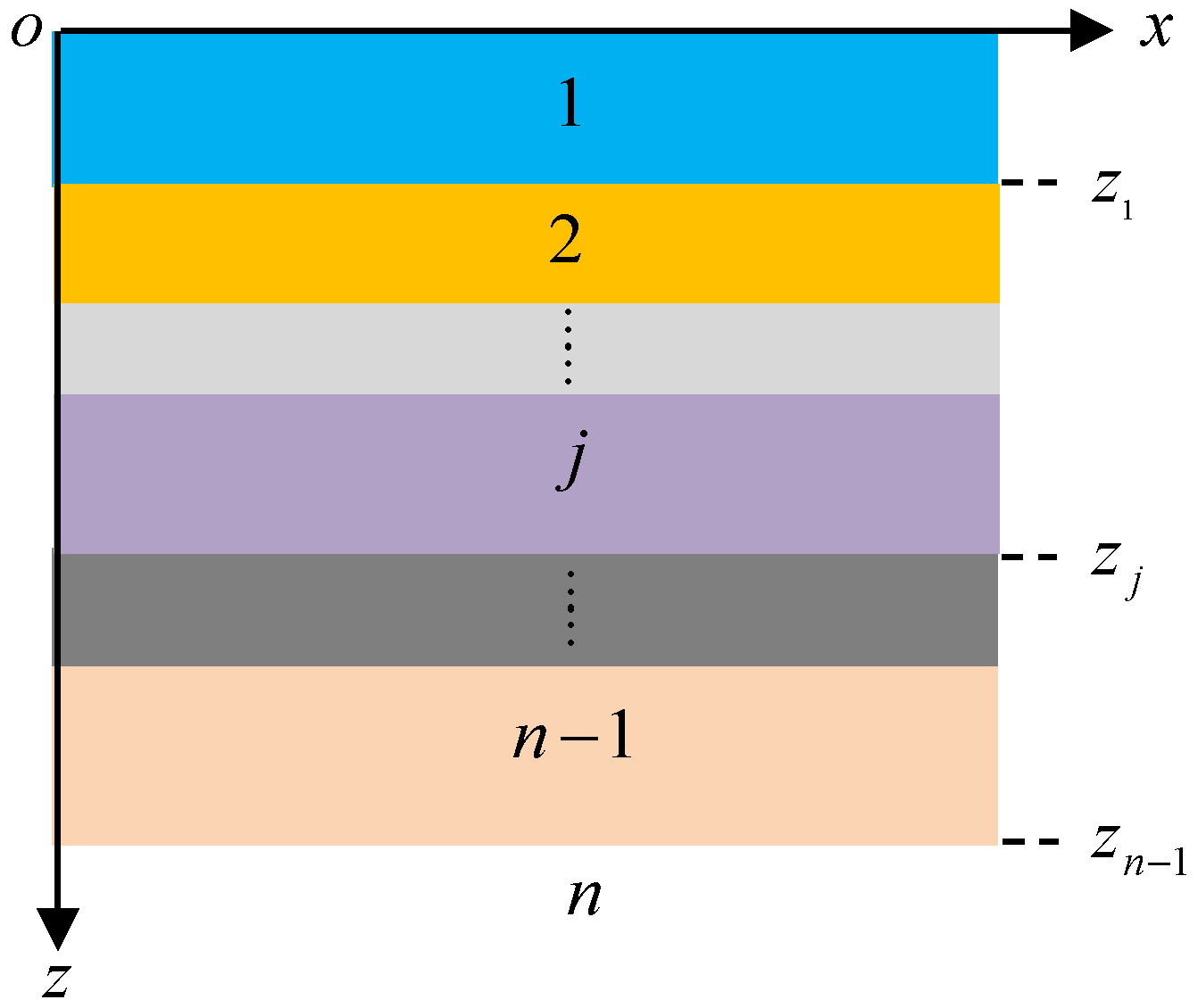
To validate this method, a two-layer arbitrary dipping model was designed (Figure 1). The parameters of each layer are listed in

Table 1. Parameters of Model 1.

Layer	h (m)	${\mathit{\lambda }}_{\mathbf{/}\mathbf{/}}$ (N/m2)	${\mathit{\lambda }}_{\mathbf{\perp }}$ (N/m2)	${\mathit{\mu }}_{\mathbf{/}\mathbf{/}}$ (N/m2)	${\mathit{\mu }}_{\mathbf{\perp }}$ (N/m2)	${\mathit{\mu }}^{\ast }$ (N/m2)	$\mathit{\rho }$ (kg/m3)
1	60	$4.0\times {10}^9$	$2.5\times {10}^9$	$1.8\times {10}^9$	$1.7\times {10}^9$	$1.5\times {10}^9$	2100
2	$\infty$	$5.0\times {10}^9$	$3.0\times {10}^9$	$3.3\times {10}^9$	$3.0\times {10}^9$	$3.2\times {10}^9$	2200

. Assuming that the normal stress at a point source outside of the interface of the first layer is a unit vector 1, solving Equation (28) based on the two-layer model yields ${\mathit{U}}_n^u={\left[\begin{array}{cc}k{\phi }_n^u& k{\psi }_n^u\end{array}\right]}^T$. The coefficients $A_n$ and $C_n$ for each layer can be calculated using the recursive equation Equation (22).

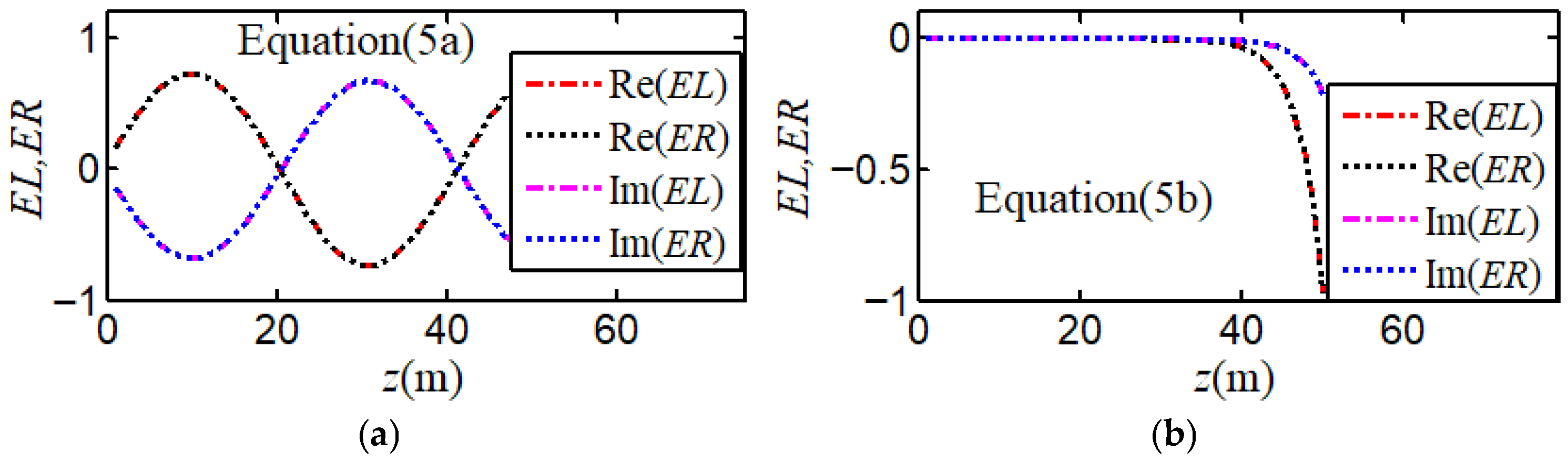
In addition, the seismic wavefield solution of the designed two-layer model is substituted directly into Equation (5) instead of Equation (10). In Equation (5a), the wave equation on the left-hand side of ${\phi }_j$ is replaced with $\Omega \left(z\right)$. In Equation (5b), the wave equation on the left-hand side of ${\psi }_j$ is replaced with ${\Psi }_j\left(z\right)$, whereas the right-hand sides of the equations remain homogeneous solutions. The results are shown in Figure 2. The seismic wave frequency is $f=50\mathrm{Hz}$, and the surface wave velocity is $c=950 \mathrm{m}\mathbf{/}\mathrm{s}$.

In Figure 2, EL denotes the normalized value of the left-hand side of the equation, and ER represents those of the right-hand side with the real $\mathrm{Re}(EL)$ and imaginary $\mathrm{Im}(EL)$ parts of $EL$. Figure 2 shows that for all values of z, the curves of $\mathrm{Im}(EL)$ and $\mathrm{Re}(ER)$ coincide, and the curves of $\mathrm{Im}(EL)$ and $\mathrm{Im}(ER)$ also coincide, which proves the equality of the wave equation Equation (5). The potential function Equation (16) satisfies the wave equation (Equation (10)) and is verified theoretically and numerically.

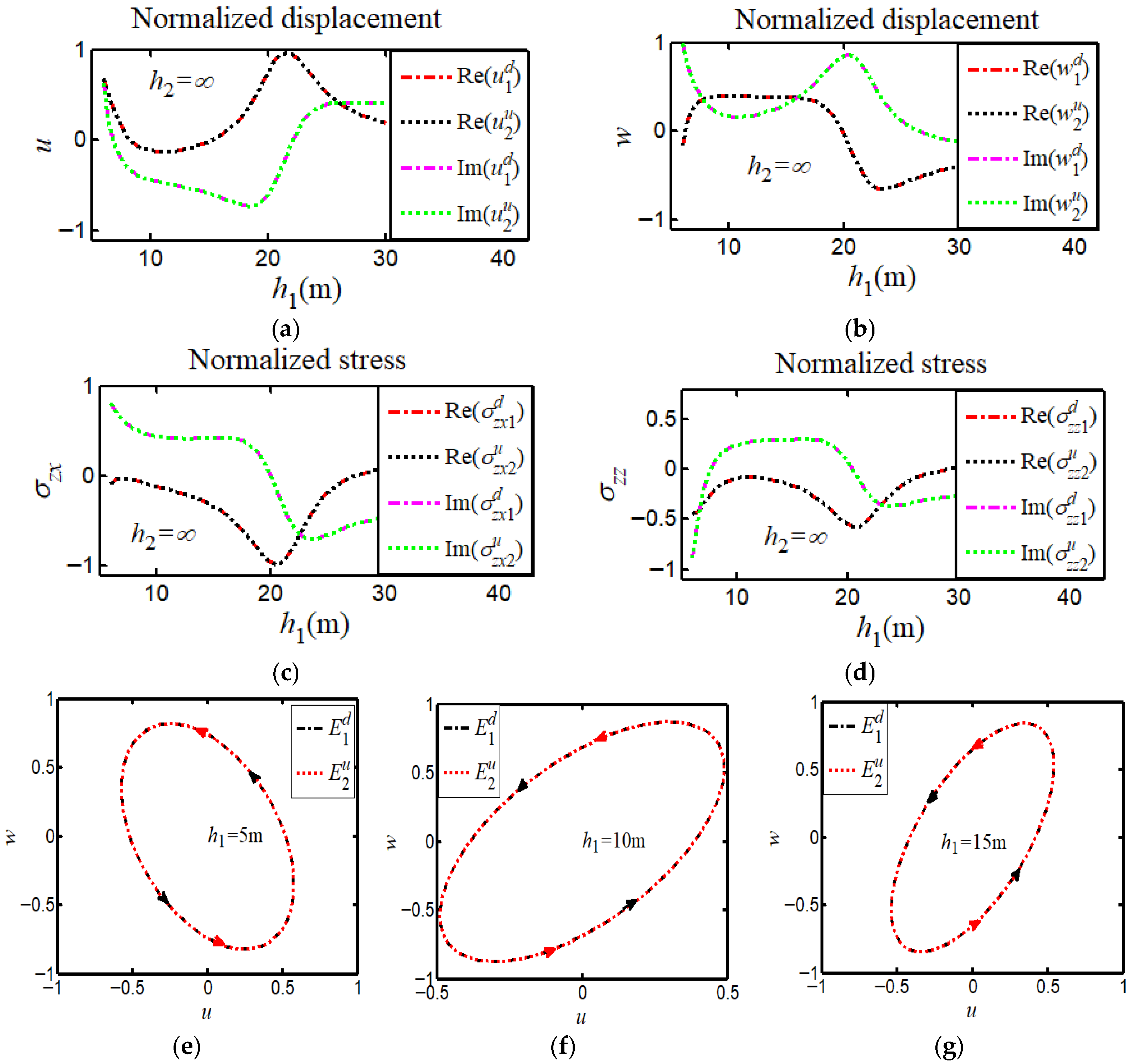
To verify whether the function solution Equation (16) satisfies the displacement and stress continuity of the seismic waves, the results from Model 1 were substituted into Equations (17) and (18) to calculate the displacement and stress above and below the second-layer interface (Figure 3). In Figure 3, $u_1^d$, $w_1^d$, ${\sigma }_{zx1}^d$, and ${\sigma }_{zz1}^d$ represent the tangential and normal displacements and stress vectors at the lower boundary of the first layer, respectively. $u_2^u$, $w_2^u$, ${\sigma }_{zx2}^u$, and ${\sigma }_{zz2}^u$ represent those on the upper boundary of the second layer. The example shows that the general solution of Equation (16) consistently satisfies the continuity of the displacement and stress on both sides of the first and second interfaces, verifying the boundary continuity condition. Figure 3e–g show that the elliptical polarization of particle motion on both sides of the interface for $h_1$ is 5 m, 10 m, and 15 m. $E_1^d$ denotes the elliptical trajectory of the displacement vector at the lower boundary of layer 1 and $E_2^u$ denotes that at the upper boundary of layer 2. Ellipse $E_1^d$ coincides with $E_2^u$ and they rotate in the same direction, indicating that particle motion on both sides of the layer 2 interface is identical. This further confirms that the computed solution satisfies the seismic boundary conditions.

6. Dispersion Characteristics of Rayleigh Waves in VTI Media

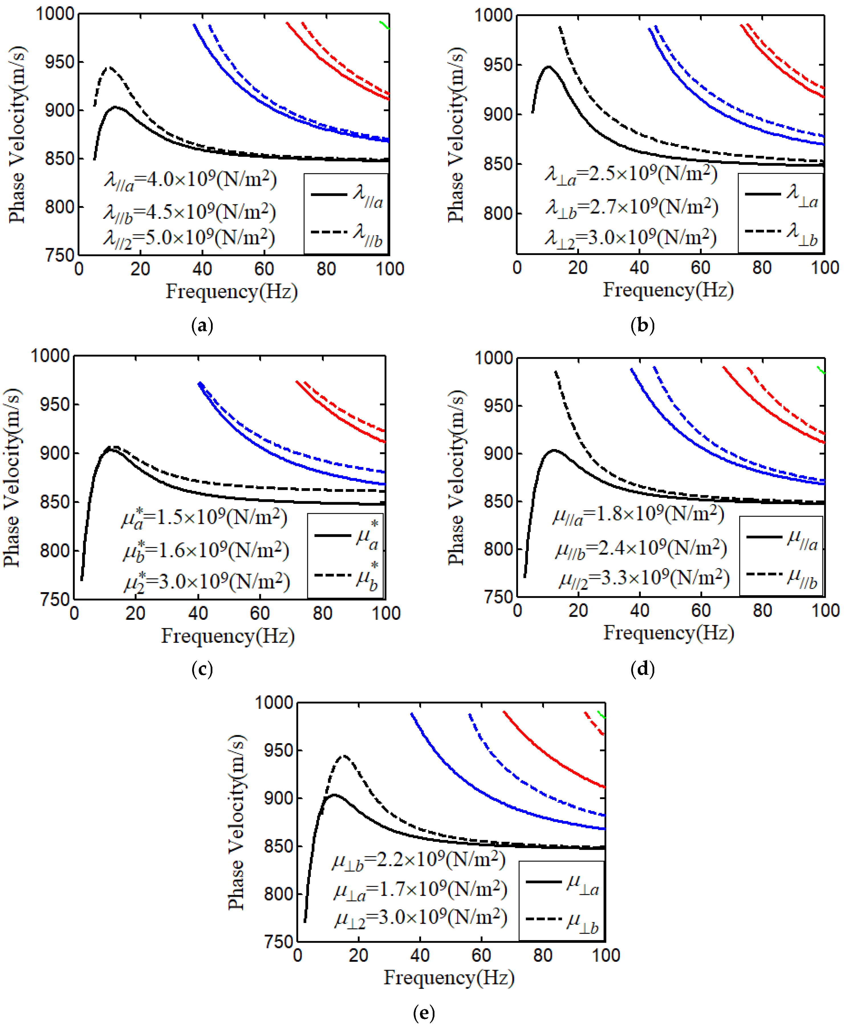
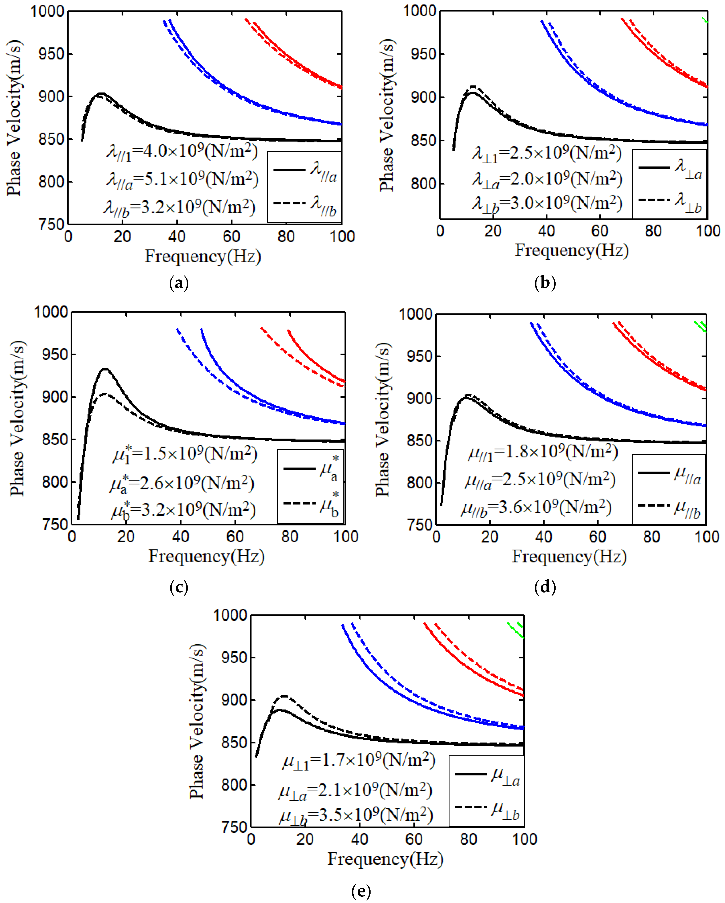
Based on Model 1, the dispersion curves of the Rayleigh waves were calculated to study the influence of the five parameters of the VTI medium (Figure 4). The thickness of layer was taken as $h_1=30 \mathrm{m}$. In each sub-figure, only one parameter of the layer was varied, whereas the other parameters remained as listed in Table 1. For example, the horizontal P-wave Lamé parameter of the first layer was taken as ${\lambda }_{\mathbf{/}\mathbf{/}1}={\lambda }_{\mathbf{/}\mathbf{/}a}={\lambda }_{\mathbf{/}\mathbf{/}b}$ in Figure 4a, and the respective dispersion curves were calculated to compare the sensitivity of the dispersion to the VTI parameters.

Figure 4 shows that changing any of the five Lamé parameters (horizontal, vertical, and shear) of the VTI media produced noticeable changes in the shape and position of the dispersion curves. The Rayleigh wave velocity is sensitive to variations in the Lamé parameters. As shown in Figure 4c, a 6% change in the Lamé parameter (${\mu }^{\ast }$) produced a relative error of up to 40% in the dispersion curve at the same frequency and mode order. The mode order of the dispersion curves is also sensitive to the VTI media parameters. In Figure 5a,d,e, three dispersion modes appeared within the computed frequency and surface wave velocity ranges, whereas Figure 5b,c show only two modes.

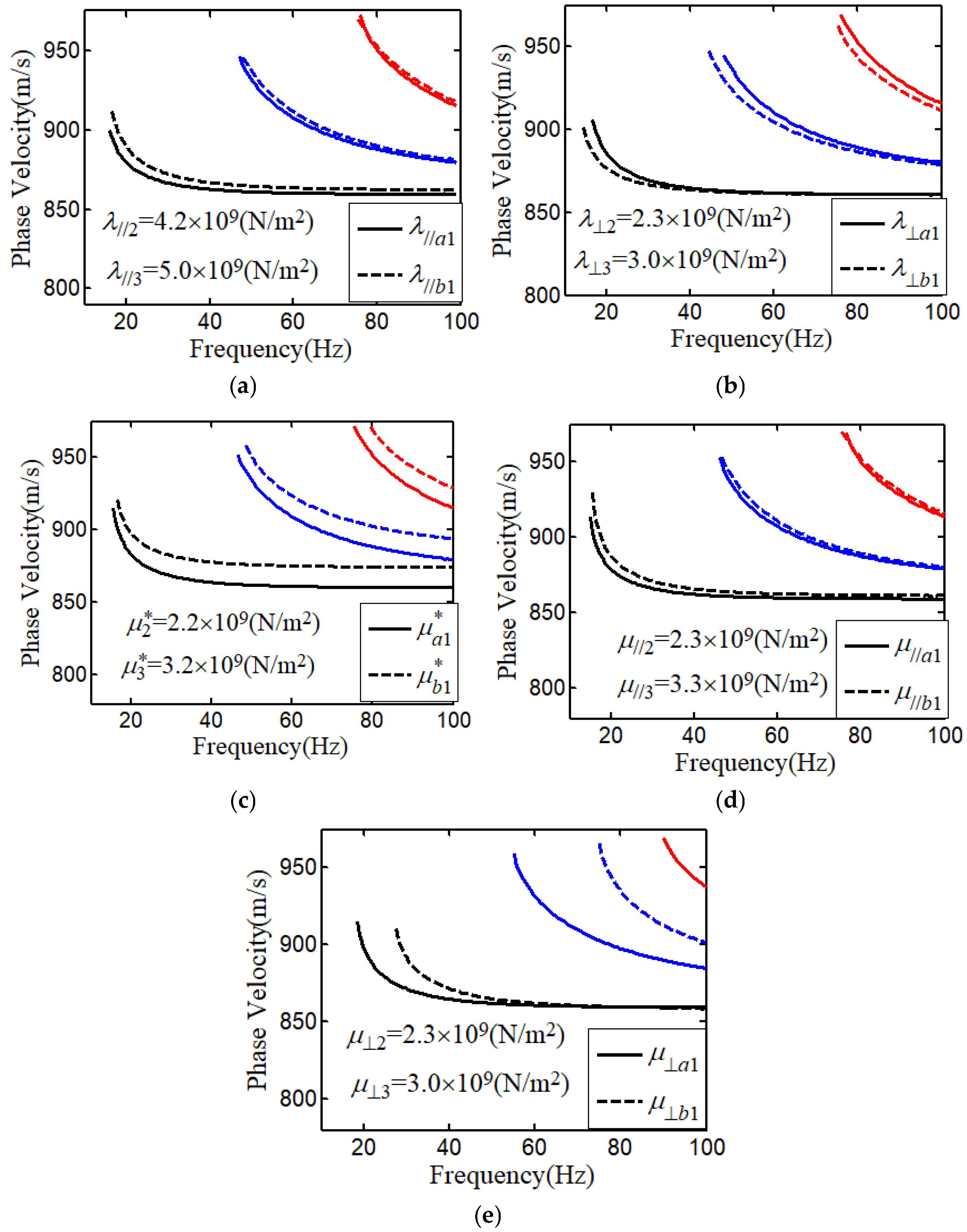
With the Lamé parameters of the first layer fixed, only one of the five Lamé parameters of the second layer varied at a time, with an increased interval between the two parameters. The results are shown in Figure 5. Figure 5 shows that increasing the interval between the Lamé parameter values for the second layer did not always increase the spacing between the dispersion curves. In some cases, the space was decreased (Figure 5a,b). The variations in the Lamé parameters of the second layer generally had a weaker impact on the dispersion curves than those of the first layer.

To further examine the dispersion characteristics of VTI media, a three-layer geological model was designed. The parameters of the three-layer VTI media are listed in

Table 2. Parameters of Model 2.

Layer	H (m)	${\mathit{\lambda }}_{\mathbf{/}\mathbf{/}}$ (N/m2)	${\mathit{\lambda }}_{\mathbf{\perp }}$ (N/m2)	${\mathit{\mu }}_{\mathbf{/}\mathbf{/}}$ (N/m2)	${\mathit{\mu }}_{\mathbf{\perp }}$ (N/m2)	${\mathit{\mu }}^{\ast }$ (N/m2)	$\mathit{\rho }$ (kg/m3)
1	30	$4.0\times {10}^9$	$2.0\times {10}^9$	$1.8\times {10}^9$	$1.7\times {10}^9$	$1.5\times {10}^9$	2000
2	25	$4.3\times {10}^9$	$2.3\times {10}^9$	$2.3\times {10}^9$	$2.4\times {10}^9$	$2.2\times {10}^9$	2100
3	$\infty$	$5.0\times {10}^9$	$3.0\times {10}^9$	$3.3\times {10}^9$	$3.0\times {10}^9$	$3.2\times {10}^9$	2200

. In

Table 3. Parameters of Model 3.

Layer	Group	${\mathit{\lambda }}_{\mathbf{/}\mathbf{/}}$ (N/m2)	${\mathit{\lambda }}_{\mathbf{\perp }}$ (N/m2)	${\mathit{\mu }}_{\mathbf{/}\mathbf{/}}$ (N/m2)	${\mathit{\mu }}_{\mathbf{\perp }}$ (N/m2)	${\mathit{\mu }}^{\ast }$ (N/m2)
Layer 1	$a_1$ $b_1$	$4.0\times {10}^9$ $4.6\times {10}^9$	$1.8\times {10}^9$ $2.7\times {10}^9$	$2.3\times {10}^9$ $3.3\times {10}^9$	$2.2\times {10}^9$ $2.7\times {10}^9$	$1.5\times {10}^9$ $1.6\times {10}^9$
Layer 2	$a_2$ $b_2$	$4.5\times {10}^9$ $5.5\times {10}^9$	$2.2\times {10}^9$ $2.5\times {10}^9$	$2.3\times {10}^9$ $2.7\times {10}^9$	$2.1\times {10}^9$ $2.6\times {10}^9$	$2.1\times {10}^9$ $2.7\times {10}^9$

, the parameters are divided into two groups for comparison. Here, a and b denote the first and second layers, respectively.

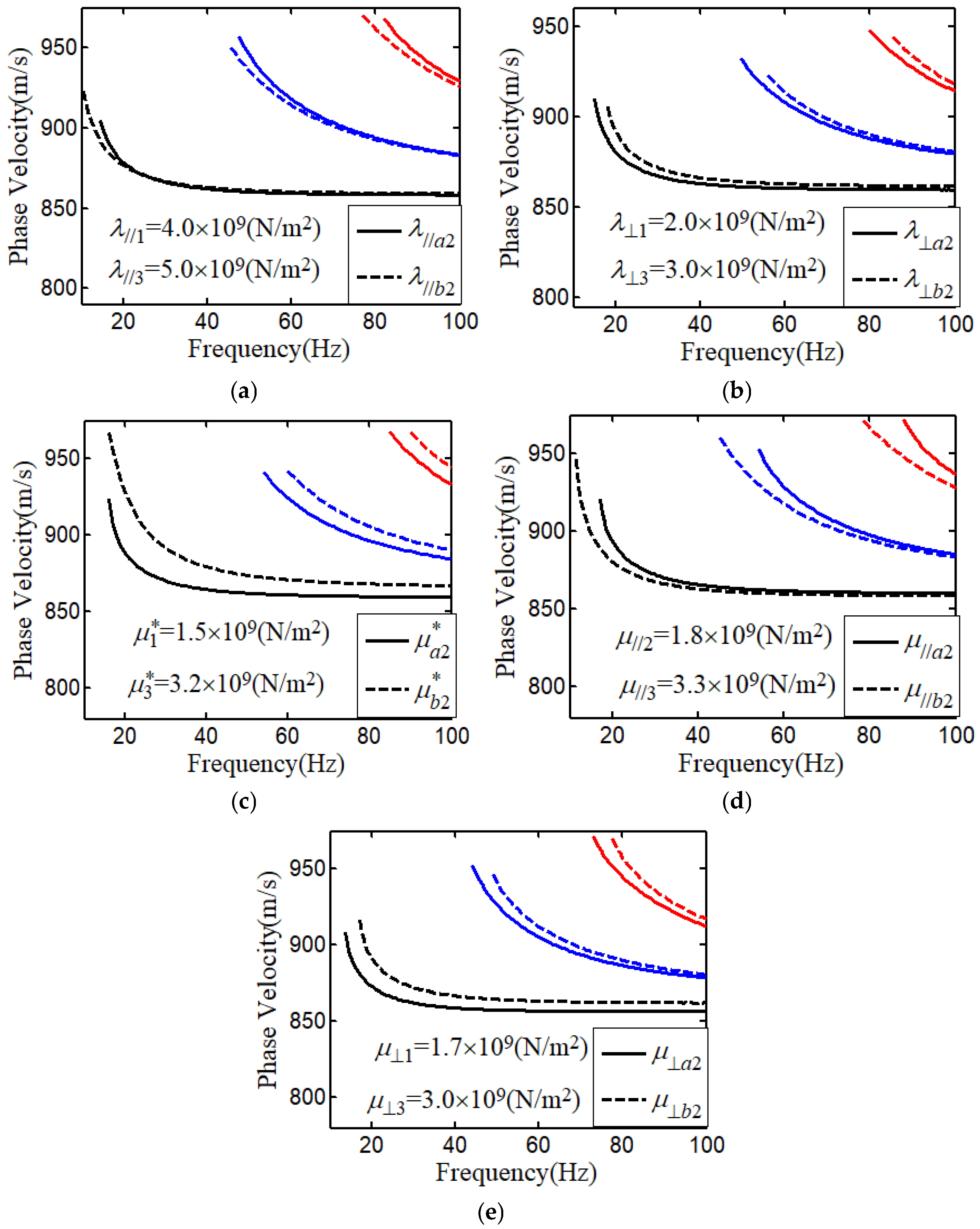
Figure 6 shows the dispersion curves obtained when only one of the five Lamé parameters of the first layer was varied. Within the same frequency and surface wave velocity range, the dispersion curves of the first layer of the VTI media exhibited noticeable differences compared to the two-layer case shown in Figure 4. There was an overall trend of weaker parameters, particularly for frequencies below $f<30 \mathrm{Hz}$. The spaces between the same-order modes of the dispersion curves narrowed. The Lamé parameters related to the P-wave and shear moduli affect the dispersion curves differently. Although the parameters ${\lambda }_{\mathbf{/}\mathbf{/}a1}$, ${\lambda }_{\mathbf{\perp }a1}$, ${\lambda }_{\mathbf{/}\mathbf{/}b1}$, and ${\lambda }_{\mathbf{\perp }b1}$ in Figure 6a,b varied considerably, the spaces between the same-order mode curves did not separate significantly. The same-order mode dispersion curves for the three shear moduli ${\mu }_{\mathbf{/}\mathbf{/}a1}$, ${\mu }_{\mathbf{\perp }a1}$, and ${\mu }_{a1}^{\ast }$ (Figure 6c–e) had relatively larger space differences. The dispersion curves of the VTI media were more sensitive to changes in the shear moduli.

Figure 7 shows the dispersion curves when only one of the five Lamé parameters of the second (middle) layer was changed. The anisotropic effects of the dispersion curves of the three-layer model were significantly stronger than those of the two-layer model (Figure 5). Compared to Figure 6, the sensitivity of the dispersion curves to the shear moduli ${\mu }_{\mathbf{/}\mathbf{/}}$, ${\mu }_{\mathbf{\perp }}$, and ${\mu }^{\ast }$ remained higher than those of other Lamé parameters with an increase in space. These calculations show that changing any of the five Lamé parameters in either the first or the second layer produces a noticeable change in the corresponding pair of dispersion curves in the same-order mode. This indicates that the dispersion response of the VTI medium is sensitive to Lamé parameters.

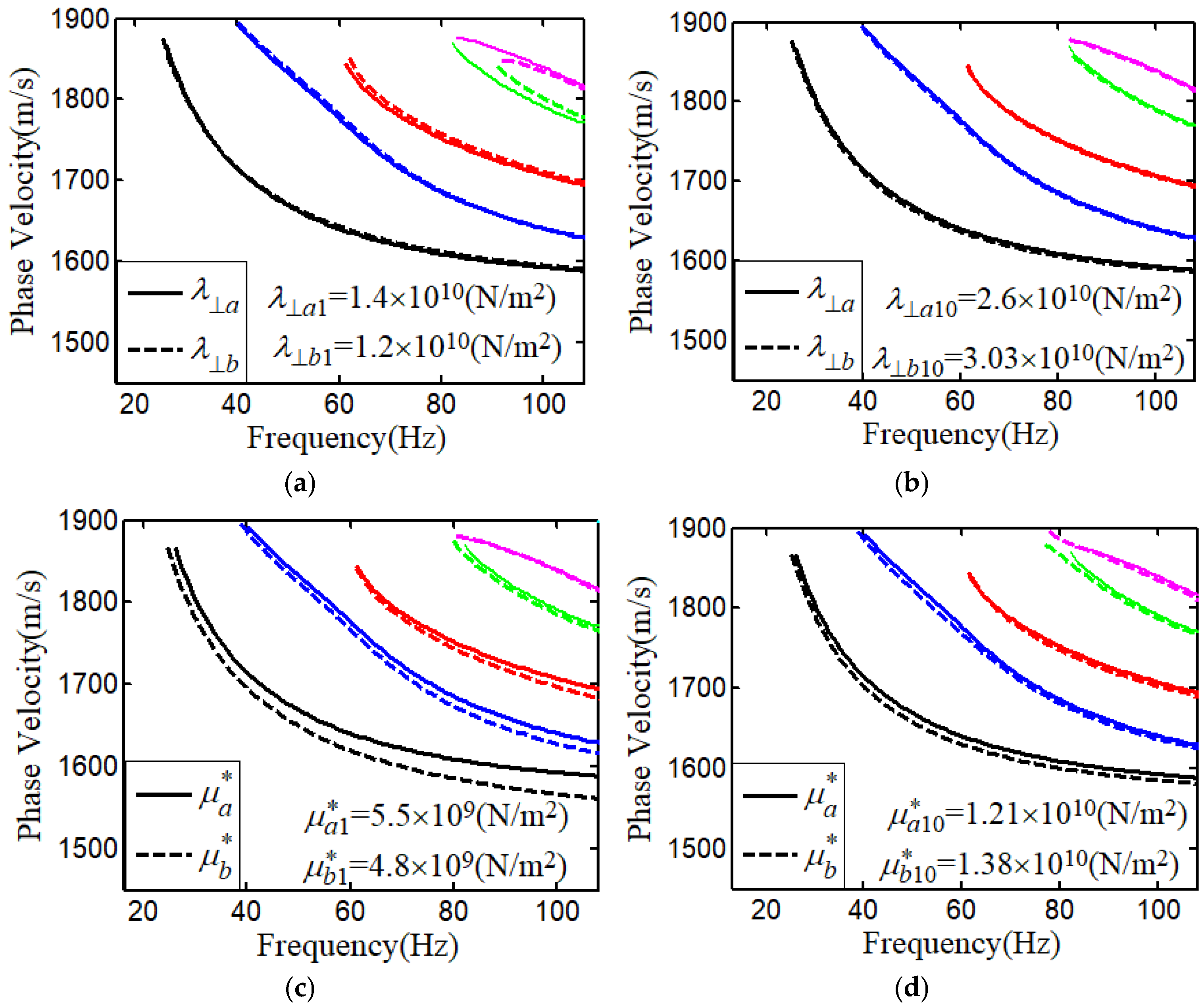
To assess the method’s scalability, we constructed a ten-layer stratigraphic model (shown in

Table 4. Stratigraphic parameters of a ten-layer model.

Lithology	H (m)	${\mathit{\lambda }}_{\mathbf{/}\mathbf{/}}$	${\mathit{\lambda }}_{\mathbf{\perp }}$	${\mathit{\mu }}_{\mathbf{/}\mathbf{/}}$	${\mathit{\mu }}_{\mathbf{\perp }}$	${\mathit{\mu }}^{\mathbf{\ast }}$	$\mathit{\rho }$
Mudstone	15	12.0	14.0	5.5	5.5	5.2	2100
Soft sand	20	13.5	16.0	6.8	5.8	5.6	2000
Shale	12	14.3	18.0	6.5	7.5	6.2.	2150
Soft mud	25	11.8	13.7	5.3	5.4	5.0	2080
Soft sand	20	13.5	16.0	6.8	5.8	5.6	2000
Shale	10	14.3	18.0	6.5	7.0	6.2	2150
Hard mud	20	18.0	20.5	7.3	7.2	7.3	2200
Hard sand	12	20.5	22.0	8.6	8.4	8.5	2320
Conglomerate	10	23.0	24.0	9.5	9.6	9.8	2380
Carbonate	$\infty$	25.5	26.0	12.5	12.1	12.2	2450

) composed of alternating thin mudstone–sandstone seabed (shown in Figure 8). Relative to the previous model, the dispersion curves for the ten-layer model are shifted toward higher values. Figure 8a,b show the effects of variation of the parameter ${\lambda }_{\mathbf{\perp }}$ in layers 1 and 10. The relative change in ${\lambda }_{\mathbf{\perp }}$ for both layers is 16.7%. These figures indicate that the vertical Lamé parameter ${\lambda }_{\mathbf{\perp }}$ in the first layer has a larger influence on the dispersion curves. As the modal order increases, the spacing between dispersion modes of the same order and frequency also increases. Figure 8c,d show the effects of variation of the parameter ${\mu }^{*}$ in layers 1 and 10. The relative change in ${\mu }^{*}$ for both layers is 14.6%. Compared with Figure 8a,b, ${\mu }^{*}$ has a noticeably greater effect on the dispersion curves than ${\lambda }_{\mathbf{\perp }}$.

7. Discussion

The algorithm’s sensitivity and stability are compared, and its runtime is measured against that of the existing Hankel function transform method. The five Lamé parameters and $\rho$ of a VTI medium are denoted by m. For each parameter $m_i$, the corresponding relative sensitivity are given by [23]:

$$S_{m_i}(f)={\displaystyle \frac{1}{c(f)}}{\displaystyle \frac{\partial c(f)}{\partial m_i}}\partial m_i\approx {\displaystyle \frac{c(f,m_i+\alpha \cdot m_i)-c(f,m_i)}{c(f,m_i)}}\times 100\%,$$

(30)

where $\alpha$ is the perturbation ratio, taken here as 10%.

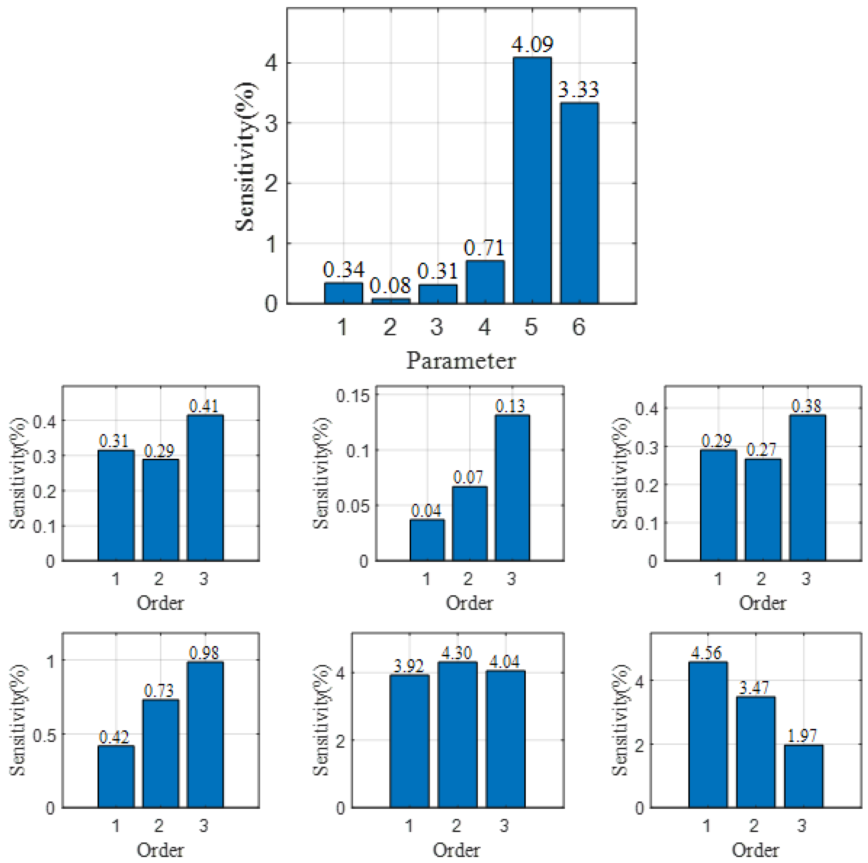
For the sensitivity tests, we use Model 2 (the three-layer VTI model). Figure 9 compares dispersion curves across modal orders, which illustrates their sensitivities to the six parameters. From these plots, the sensitivities, ranked from largest to smallest, are ${\mu }^{\ast }$, $\rho$, ${\mu }_{\mathbf{\perp }}$, ${\lambda }_{\mathbf{/}\mathbf{/}}$, ${\mu }_{\mathbf{/}\mathbf{/}}$, and ${\lambda }_{\mathbf{\perp }}$.

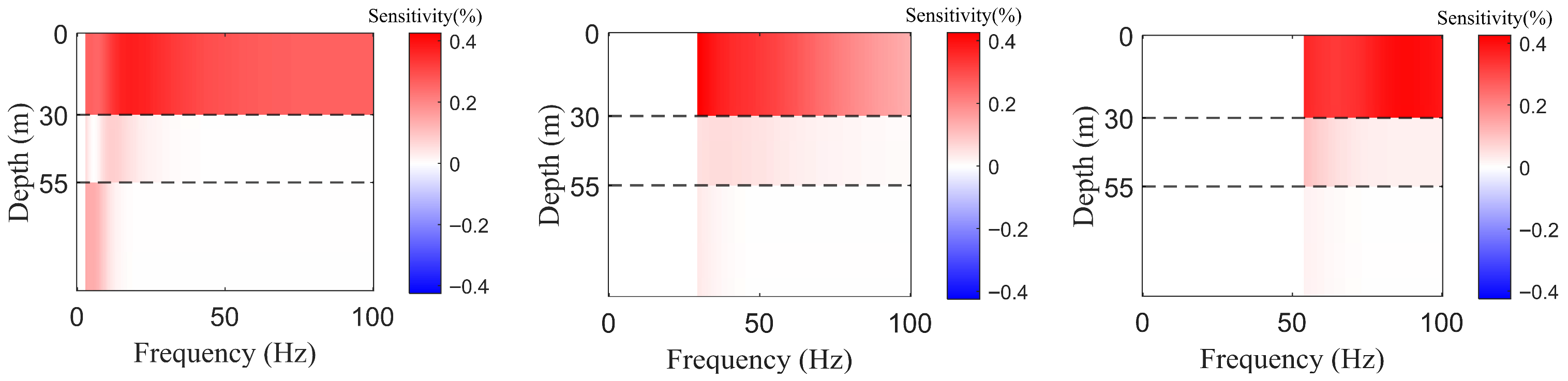
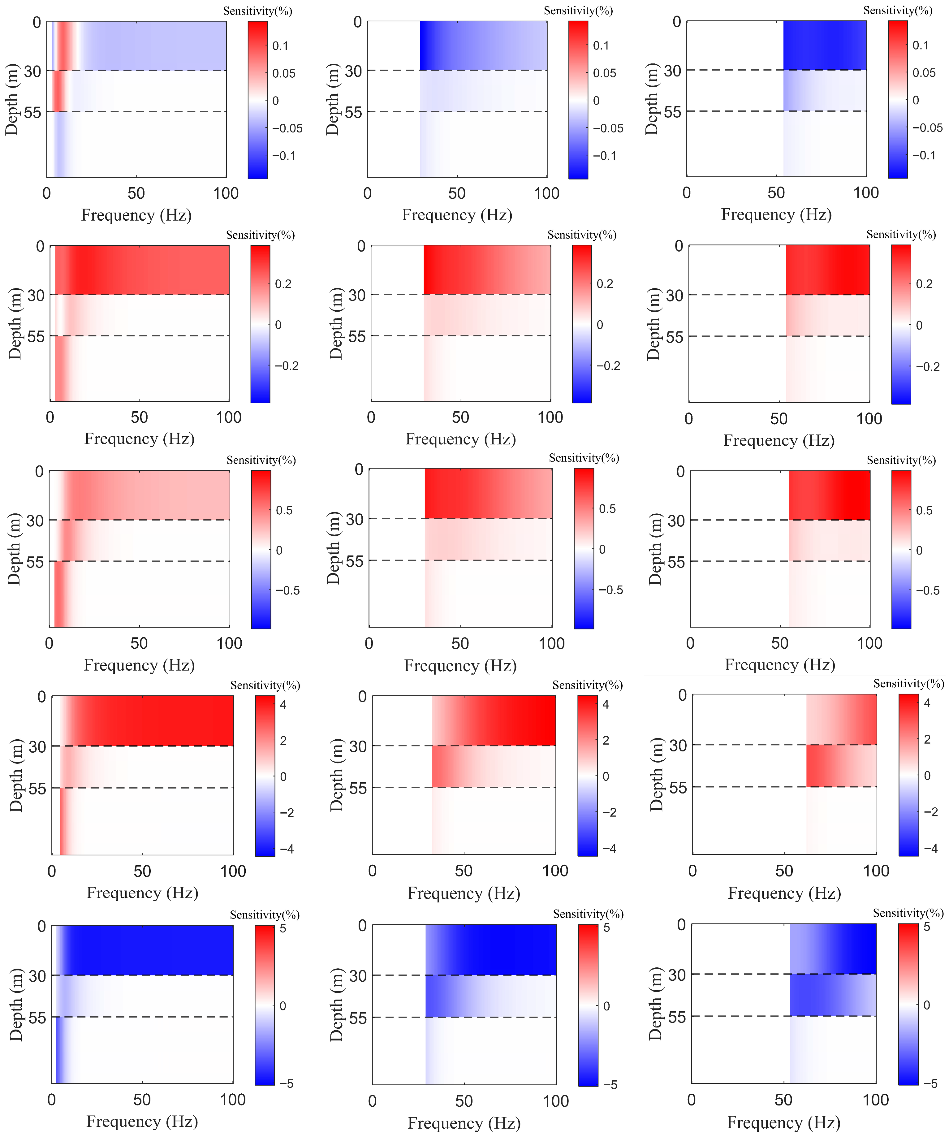
Figure 10 shows how sensitivity varies with frequency and layer depth. Overall, sensitivity is strongest in the shallow layers. With increasing depth, sensitivity shifts predominantly to the low-frequency band, reflecting the Rayleigh wave characteristic. The modes show clear complementarity, as higher-order modes are more sensitive to shallow parameters at higher frequencies while lower-order modes are more sensitive to deeper layers at low frequencies. From the signs of the sensitivities, ${\lambda }_{\mathbf{/}\mathbf{/}}$, ${\lambda }_{\mathbf{\perp }}$, ${\mu }_{\mathbf{/}\mathbf{/}}$, ${\mu }_{\mathbf{\perp }}$, and ${\mu }^{\ast }$ are generally positively correlated with phase velocity (increases in these parameters raise phase velocity), whereas ${\lambda }_{\mathbf{\perp }}$ and $\rho$ exhibit negative correlations. This directional information provides direct and useful prior constraints for inversion.

Based on the sensitivity analysis above, we draw several conclusions. Within the target frequency band and modal configuration, parameters to which the dispersion curves are most sensitive should be prioritized in inversion. Parameters with weak sensitivity should be constrained using stronger priors. Alternatively, those weakly sensitive parameters can be jointly inverted with other observables. Moreover, multi-mode joint inversion substantially improves the resolvability of parameters at different depths.

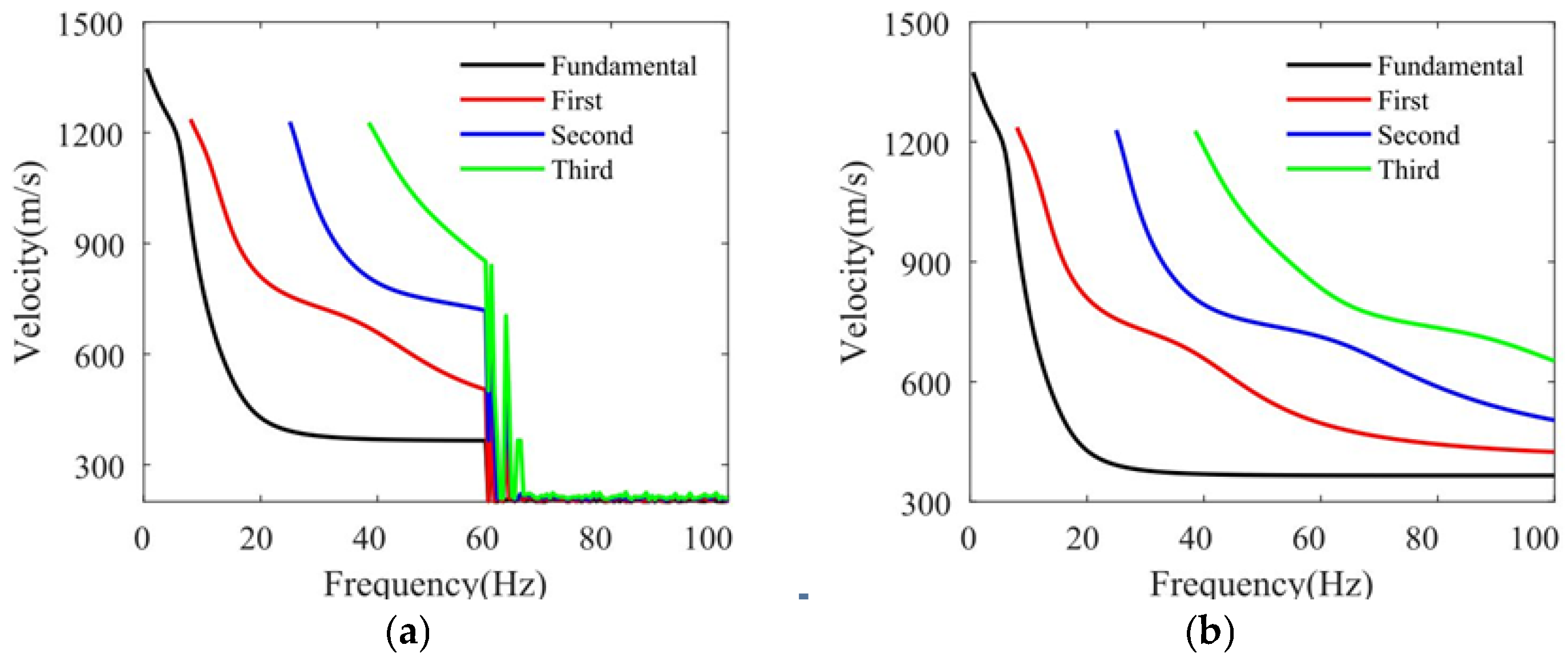
A common challenge in computing dispersion curves is maintaining numerical stability. Concretely, the intermediate state vector is normalized by its norm, and the scaling factor is accumulated after each layer’s recursive update. All subsequent recursions are then carried out on this normalized scale. The key property of this procedure is that scaling alters the numerical magnitude of the determinant/discriminant function but does not change its zeros, so the physical roots of the dispersion relation remain unaffected. Meanwhile, this approach strongly suppresses exponential overflow and reduces the accumulation of rounding errors at high frequencies. Figure 11a shows the computational result without normalizing and improvement. When the frequency $f>60$, the dispersion curves can no longer be obtained. However, after normalizing improvement, the dispersion curve can still be stably obtained for frequency $f>100$, as shown in Figure 11b.

When forming the dispersion equation, this derived method requires only the recursive updates plus the evaluation of a single 2 × 2 determinant. In contrast, existing decoupling algorithms based on Hankel transforms construct the dispersion equation by setting the determinants of all boundary equation coefficient matrices to zero. If there are n layer interfaces, the total number of unknown coefficients is N = 4n − 2. For a ten-layer model, this gives 42 unknowns and a 42 × 42 determinant. Dispersion equations become unwieldy for models with many layers, and computing such large determinants is computationally expensive. Apart from the recursion, this derived algorithm avoids that cost by needing only a single 2 × 2 determinant evaluation.

To quantify this advantage, we compare the time required to evaluate the dispersion equation value. Results are shown in

Table 5. Comparison of computation time.

Layers	3	10	15	20	25
N-Hank	$7\times 7$	$42\times 42$	$58\times 58$	$86\times 86$	$128\times 128$
t-Hank(S)	0.254	1.259	3.001	5.761	9.951
t-Non-d(S)	0.201	0.696	1.128	1.561	2.340

and report times for 10,000 evaluations. Matrix elements in both methods are assembled using the approach described here. Column t_Nond(S) gives the time our method requires to evaluate the dispersion equation value, while N_Hank reports the time to compute the Hankel-based dispersion equation value. As the number of layer interfaces increases, the time to compute the dispersion equation value using the Hankel transform approach grows rapidly.

This non-decoupled algorithm uses the homogeneous P-wave solution as the source term in the SV-wave equation and the homogeneous SV-wave solution as the source term in the P-wave equation, which provides a fully coupled analytical treatment for VTI media. No additional restrictive assumptions are introduced during the derivation, so this method is broadly applicable. In short, it constitutes a general algorithm for non-decoupled analytical computation in VTI media.

8. Conclusions

This study derived the dispersion equations for Rayleigh waves in multi-layered VTI media. The Rayleigh wave dispersion equations for VTI media were articulated, and the analytical computation of the Rayleigh wavefield and its dispersion curves within the VTI media was accomplished without the special decoupling process often required by previous approaches. Sensitivity studies were conducted on the dispersion response of Rayleigh waves to five VTI layer parameters. The numerical results indicate that the modification of any of the five Lamé parameters causes changes in both the shape and position of the dispersion curves. The parameters of the lower layers had less impact on the dispersion curves than those at the upper interface, illustrating the pronounced sensitivity of Rayleigh wave velocities to variations in the Lamé parameters in VTI media. As no simplifying assumptions or model restrictions were imposed during the development of the solution and dispersion equations, the analytical solution can be applied to any configuration of multi-layered VTI strata. Based on the derived dispersion equation, Rayleigh wave dispersion curves in VTI media can be computed. These equations will be applied to invert anisotropic parameters for VTI media.

References

1. Zhao, M.; Barbosa, J.M.O.; Metrikine, A.V.; Dalen, K.N. Semi-analytical solution for the 3D response of a tunnel embedded in an elastic half-space subject to seismic waves. Soil Dyn. Earthq. Eng. 2023, 174, 108171. [Google Scholar] [CrossRef] [Scilit]
2. Levin, F.K. The reflection, refraction, and diffraction of waves in media with an elliptical velocity dependence. Geophysics 1978, 43, 528–537. [Google Scholar] [CrossRef] [Scilit]
3. Thomsen, L. Weak elastic anisotropy. Geophysics 1986, 51, 1954–1966. [Google Scholar] [CrossRef] [Scilit]
4. Sena, A.G. Seismic traveltime equations for azimuthally anisotropic and isotropic media: Estimation of interval elastic properties. Geophysics 1991, 56, 2090–2101. [Google Scholar] [CrossRef] [Scilit]
5. Tsvankin, I. P-wave signatures and notation for transversely isotropic media: An overview. Geophysics 1996, 61, 467–483. [Google Scholar] [CrossRef] [Scilit]
6. Alkhalifah, T. An acoustic wave equation for anisotropic media. Geophysics 2000, 65, 1239–1250. [Google Scholar] [CrossRef] [Scilit]
7. Bagheri, A.; Greenhalgh, S.; Khojasteh, A.; Rahimian, M. Dispersion of Rayleigh, Scholte, Stoneley and Love waves in a model consisting of a liquid layer overlying a two-layer transversely isotropic solid medium. Geophys. J. Int. 2015, 203, 195–212. [Google Scholar] [CrossRef] [Scilit]
8. Zuo, J.; Niu, F.; Liu, L.; Da, S.; Zhang, H.; Yang, J.; Zhang, L.; Zhao, Y. 3D Anisotropic P- and S-Mode Wavefields Separation in 3D Elastic Reverse-Time Migration. Surv. Geophys. 2022, 43, 673–701. [Google Scholar] [CrossRef] [Scilit]
9. Stoneley, R. The Seismological Implications of Aeolotropy in Continental Structure. Geophys. J. Int. 1949, 5, 343–353. [Google Scholar] [CrossRef] [Scilit]
10. Buchwald, V.T. Rayleigh Waves in Transversely Isotropic Media. Q. J. Mech. Appl. Math. 1961, 4, 293–318. [Google Scholar] [CrossRef] [Scilit]
11. Ji, G.; Zhang, P.; Wu, R.; Guo, L.; Hu, Z.; Wu, H. Calculation method and characteristic analysis of dispersion curves of Rayleigh channel waves in transversely isotropic media. Geophysics 2020, 85, C187–C198. [Google Scholar] [CrossRef] [Scilit]
12. Sharma, M.D.; Kumar, R.; Gogna, M.L. Surface wave propagation in a transversely isotropic elastic layer overlying a liquid saturated porous solid half-space and lying under the uniform layer of liquid. Pure Appl. Geophys. 1990, 133, 523–539. [Google Scholar] [CrossRef] [Scilit]
13. Sharma, M.D. Dispersion in oceanic crust during earthquake preparation. Int. J. Solids Struct. 1999, 36, 3469–3482. [Google Scholar] [CrossRef] [Scilit]
14. Xi, C.; Xia, J.; Mi, B.; Dai, T.; Liu, Y.; Ning, L. Modified frequency-Bessel transform method for dispersion imaging of Rayleigh waves from ambient seismic noise. Geophys. J. Int. 2021, 225, 1271–1280. [Google Scholar] [CrossRef] [Scilit]
15. Ba, Z.; An, D. Seismic response of a 3-D canyon in a multilayered TI half-space modelled by an indirect boundary integral equation method. Geophys. J. Int. 2019, 217, 1949–1973. [Google Scholar] [CrossRef] [Scilit]
16. Rahimian, M.; Eskandari-Ghadi, M.; Park, R.Y.S.; Khojasteh, A. Elastodynamic Potential Method for Transversely Isotropic Solid. J. Eng. Mech. 2007, 133, 1134–1145. [Google Scholar] [CrossRef] [Scilit]
17. Khojasteh, A.; Rahimian, M. Three-dimensional dynamic Green’s functions in transversely isotropic bi-materials. Int. J. Solid Struct. 2008, 45, 4952–4972. [Google Scholar] [CrossRef] [Scilit]
18. Khojasteh, A.; Rahimian, M.; Eskandari, M. Asymmetric wave propagation in a transversely isotropic half-space in displacement potentials. Int. J. Eng. Sci. 2008, 46, 690–710. [Google Scholar] [CrossRef] [Scilit]
19. Khojasteh, A.; Rahimian, M.; Eskandari, M. Three-dimensional dynamic Green’s functions in transversely isotropic tri-materials. Appl. Math. Model. 2013, 37, 3164–3180. [Google Scholar] [CrossRef] [Scilit]
20. Chen, X. A systematic and efficient method of computing normal modes for multilayered half-space. Geophys. J. Int. 1993, 115, 391–409. [Google Scholar] [CrossRef] [Scilit]
21. Liu, X.; Fan, Y. On the characteristics of high-frequency Rayleigh waves in stratified half-space. Geophys. J. Int. 2012, 190, 1041–1057. [Google Scholar] [CrossRef] [Scilit]
22. Naeeni, M.R.; Pan, E.; Eskandari-Ghadi, M.; Han, S. Semi-analytical solution for the elastic wave propagation due to a dislocation source in a transversely isotropic half-space. Geophys. J. Int. 2023, 234, 1363–1388. [Google Scholar] [CrossRef] [Scilit]
23. Feng, S.; Sugiyama, T.; Yamanaka, H. Effectiveness of multi-mode surface wave inversion in shallow engineering site investigations. Explor. Geophys. 2005, 36, 26–33. [Google Scholar] [CrossRef] [Scilit]
Figure 1. Stratified VTI medium formation model. Different colors represent different layers.
Mathematics 14 00700 g001
Figure 2. Numerical verification in VTI medium. (a) Verification using Equation (5a); (b) Verification using Equation (5a). Re ( E L ) and Im ( E L ) denote the real and imaginary normalized value of the left side of Equation (5); Re ( E R ) and Im ( E R ) denote the real and imaginary normalized value of the right side of Equation (5).
Mathematics 14 00700 g002
Figure 3. Validation of boundary conditions in seismic wavefield modeling for VTI media. (a,b) are the normalized displacements; (c,d) are the normalized stress; (e–g) elliptical polarization of particle motion on both sides of the interface for h 1 is 5 m, 10 m, and 15 m. Re ( u 1 d ) , Re ( w 1 d ) , Im ( u 1 d ) , and Im ( w 1 d ) are the real and imaginary parts of the tangential and normal displacements of the lower interface of layer 1; Re ( σ z x 1 d ) , Re ( σ z z 1 d ) , Im ( σ z x 1 d ) , and Re ( σ z z 1 d ) are the real and imaginary parts of the tangential and normal displacements of the upper interface of layer 2; Re ( σ z x 1 d ) , Re ( σ z z 1 d ) , Im ( σ z x 1 d ) , and Im ( σ z z 1 d ) are the real and imaginary parts of the tangential and normal stresses on the lower interface of layer 1; Re ( σ z x 2 u ) , Re ( σ z z 2 u ) , Im ( σ z x 2 u ) , and Re ( σ z z 2 u ) are the real and imaginary parts of the tangential and normal stresses on the upper interface of layer 2.
Mathematics 14 00700 g003
Figure 4. Dispersion curves for elastic parameters in the upper layer of a two-layer VTI medium. (a,b) Dispersion responses of horizontal and vertical Lamé parameters ( λ / / 1 and λ ⊥ 1 ) for layer 1, respectively; (c–e) dispersion responses of shear, parallel, and vertical shear Lamé parameters ( μ 1 ∗ , μ / / 1 , and μ ⊥ 1 ) for layer 1, respectively; (d) dispersion response of parallel shear Lamé parameter for layer 1 medium; (e) dispersion response of vertical shear Lamé parameter for layer 1 medium. Black lines: fundamental mode of Rayleigh wave; Blue lines: first-mode of Rayleigh wave; Red lines: second-mode of Rayleigh wave.
Mathematics 14 00700 g004
Figure 5. Dispersion curves of lower-layer elastic parameters of two-layer VTI medium. (a,b) Dispersion curves of the horizontal ( λ / / 2 ) and vertical ( λ ⊥ 2 ) Lamé coefficient of the second layer, respectively; (c–e) dispersion curves of the shear ( μ 2 ∗ ), horizontal shear ( μ / / 2 ), and vertical shear ( μ ⊥ 2 ) Lamé coefficient of the second layer, respectively. Black lines: fundamental mode of Rayleigh wave; Blue lines: first-mode of Rayleigh wave; Red lines: second-mode of Rayleigh wave.
Mathematics 14 00700 g005
Figure 6. Dispersion curves of the first (upper) layer parameters of three-layer VTI medium. (a,b) Dispersion curves of the horizontal ( λ / / 1 ) and vertical ( λ ⊥ 1 ) Lamé coefficient of the second layer, respectively; (c–e) dispersion curves of the shear ( μ 1 ∗ ), horizontal shear ( μ / / 1 ), and vertical shear ( μ ⊥ 1 ) Lamé coefficient of the second layer, respectively. Black lines: fundamental mode of Rayleigh wave; Blue lines: first-mode of Rayleigh wave; Red lines: second-mode of Rayleigh wave.
Mathematics 14 00700 g006
Figure 7. Dispersion curves of the second (middle) layer of Model 3. (a,b) Dispersion curves of the horizontal ( λ / / 2 ) and vertical ( λ ⊥ 2 ) Lamé coefficient of the second layer, respectively; (c–e) dispersion curves of the shear ( μ 2 ∗ ), horizontal shear ( μ / / 2 ), and vertical shear ( μ ⊥ 2 ) Lamé coefficient of the second layer, respectively. Black lines: fundamental mode of Rayleigh wave; Blue lines: first-mode of Rayleigh wave; Red lines: second-mode of Rayleigh wave.
Mathematics 14 00700 g007
Figure 8. Dispersion curves of Model 4. (a,b) Effects of variation of the parameter λ ⊥ in layers 1 and 10. (c,d) Effects of variation of the parameter μ * in layers 1 and 10. Black lines: fundamental mode of Rayleigh wave; Blue lines: first-mode of Rayleigh wave; Red lines: second-mode of Rayleigh wave; Green lines: Third-mode of Rayleigh wave; Pink lines: Fourth-mode of Rayleigh wave.
Mathematics 14 00700 g008
Figure 9. Comparisons of the sensitivity of the first three modal dispersion curves to the six anisotropic parameters ( λ / / , λ ⊥ , μ ∗ , λ / / , μ / / , and ρ ).
Mathematics 14 00700 g009
Figure 10. Variation of the sensitivities of the first three modal dispersion curves to the six anisotropic parameters ( λ / / , λ ⊥ , μ ∗ , λ / / , μ / / , and ρ ,) with frequency and depth.
Mathematics 14 00700 g010aMathematics 14 00700 g010b
Figure 11. Stability comparison. (a) Before improvement; (b) after improvement.
Mathematics 14 00700 g011