Numerical Solution of Integral Algebraic Equations with Singular Points Using the Least Squares Method

Abstract

We conduct a numerical study of integral algebraic equations (IAEs) with singular points, which pose significant challenges for standard computational methods. The presence of singular points often renders classical discretization schemes unstable and inaccurate. This work explores the reformulation of such problems using a least squares framework to restore numerical stability. By recasting the singular IAE as a minimization problem, the least squares method effectively handles the non-integrability and ill-conditioning inherent in direct approaches. We provide a numerical analysis of the proposed scheme and present results from several test cases, demonstrating its superior performance in terms of the convergence rate and solution quality compared to conventional methods. Our findings establish the least squares method as a viable and effective tool for solving singular IAEs.

1. Introduction

Integral algebraic equations (IAEs) represent an important class of mathematical objects. They arise when constructing models of natural and technical processes with memory and balance relations. These models are formulated as a set of Volterra integral equations of the first and second kind, along with finite algebraic equations, interconnected via the components of the desired vector-function. They take the form of a system of integral equations with an identically singular matrix in the principal part. Currently, such models are found in many applied fields, including the theory of viscoelasticity with material memory effects, population dynamics in biology, economic modeling, and optimal control problems with aftereffect.

The development of numerical methods for solving IAEs has been associated with significant difficulties. Constructive theorems on the solvability of IAEs were lacking, and solution methods were developed in parallel with the construction of the qualitative theory. The theoretical foundations for singular systems of integral equations are rooted in earlier work on differential-algebraic equations (DAEs). Key analytical tools, such as left regularizing operators, the analysis of matrix pencils, and the formalization of singular points, are directly adapted from DAE theory to characterize the solvability and structural properties of IAEs. Consequently, the numerical analysis and classification of IAEs, including the challenges posed by singularities and high index, inherit their core methodology and terminology from the well-developed corpus of DAE research, providing a vital theoretical bridge for investigating these complex integral systems.

Early foundational contributions in this area include the works of Chistyakov [1] on singular ordinary differential systems and their integral analogues, and the monograph by Hairer et al. [2] on numerical methods for singular systems. A pivotal connection was established by Gear, whose paper [3] formally linked the theory of DAEs, including the concept of the index, to integral–algebraic equations (IAEs). This theoretical framework was expanded in the monographs [4,5] on algebraic-differential systems. The development of numerical analysis for these problems progressed along two parallel tracks: integral equations and DAEs. For Volterra-type equations, the monographs by Brunner [6,7] on collocation methods and Volterra integral equations, respectively, provide a general foundation. Within the specific context of IAEs, Kauthen [8,9] pioneered the analysis of polynomial spline collocation methods for index-1 equations. This line of inquiry was significantly advanced in the theoretical work of Liang and Brunner [10,11], which established a comprehensive framework for collocation methods applied to IAEs. Concurrently, the projector-based analysis of DAEs, as detailed in the monographs by Lamour et al. [12] and Kunkel and Mehrmann [13], provides essential tools for understanding the related singular structures. Specific investigations into the properties of linear Volterra integro-algebraic systems have been continued by Chistyakov and colleagues. This includes studies on solvability and numerical methods [14], and most recently, an examination of singular points and solvability conditions [15]. Together, this body of literature forms the core theoretical and numerical basis for the study of singular integral and integro-algebraic equations.

Generally, in the works on constructing numerical methods for solving IAEs, three main directions can be conditionally distinguished: (I) Finite-difference methods [1,16]. Here, within the framework of existence theorems, conditions for stability and convergence of first and higher orders have been obtained. (II) Methods based on collocation. The articles and monographs [7,8] laid the foundation for the theory of collocation methods for IAEs. They present the qualitative theory of IAEs and the theory of numerical methods, including convergence analysis. A major contribution to this direction are the works [17,18,19,20,21] on spline collocation and spectral methods. In particular, it is shown that collocation methods allow solving Hessenberg-type IAEs with a high index. (III) Methods based on variational principles. Notable works here include [22,23].

This article is a continuation of the work on applying the least squares method (LSM) for solving degenerate problems (see [14,22]). We focus our research on IAEs with singular points in the domain. The development of stable numerical methods for IAEs with singular points is highly relevant. In applied problems, the presence of singular points can lead to a significant loss of accuracy or loss of convergence of step-by-step methods (in particular, finite difference schemes). The proposed least squares-based approach allows these difficulties to be partially circumvented, ensuring global approximation of the solution and stability even in the presence of singularities. Thus, this work aims to address an important problem in computational mathematics with applications in natural and technical sciences.

Similar to previous works, the problem of solving IAEs is replaced by the problem of minimizing a residual functional in Sobolev spaces. The article formalizes the concept of a singular point of IAEs and considers a number of examples with singular points, which are solved by the LSM followed by an analysis of the numerical processes. Unlike finite-difference and spline-collocation methods, the LSM allows searching for the solution not step-by-step but globally, eliminating potential instability or halting that arises when grid nodes coincide with or are close to singular points. A comparison of these results with the application of the finite-difference method from [1] is provided.

The brief review given above by no means claims to be exhaustive and provides only reference points for orientation within the vast accumulated material.

The article is structured as follows. In Section 2, we formally state the IAE problem and introduce basic concepts and definitions. Section 3 is devoted to key theoretical tools, including ways of formalizing the concept of a singular point. In Section 4, we present the main theorem on the solvability of IAEs. Section 5 describes the proposed numerical method based on LSM, including the form of the residual functional and coordinate functions. The results of the numerical experiments for several test cases with singular points are presented and analyzed in Section 6. Finally, Section 7 provides a general discussion of the results.

2. Problem Statement

We consider systems of Volterra integral equations of the form

$$({\mathrm{\Lambda }}_0+\mathcal{V})x=A\left(t\right)x\left(t\right)+\underset{\alpha }{\overset{t}{\int }}K(t,s)x\left(s\right)ds=\varphi \left(t\right),t\in T=[\alpha ,\beta ],$$

(1)

where $\mathcal{V}$ is the Volterra operator, the symbol ${\mathrm{\Lambda }}_i,i=0,1,\dots ,$ denotes a differential operator in which the zero power of the operator $(d/dt)$ is assumed to be the identity operator, $A\left(t\right),K(t,s)$ are given $(n\times n)$ matrices, $x\equiv x\left(t\right)$ is the unknown vector-function, and $\varphi \left(t\right)$ is a given vector-function.

It is assumed that, at a minimum, the matrices $A\left(t\right),K(t,s)$ and the vector-function $\varphi \left(t\right)$ are continuous in their domains, and the following condition holds:

$$\det A\left(t\right)=0\forall t\in T.$$

(2)

The smoothness requirements will be specified separately in the statements of definitions and assertions. Systems of the form (1) satisfying condition (2) are currently referred to as integro-algebraic equations (IAEs).

By the solution of the IAE (1), we understand any vector-function $x\left(t\right)\in \mathbf{C}\left(T\right)$ that satisfies the IAE identically on T upon substitution.

This article pays particular attention to IAEs with singular points. Informally, by a singular point of the IAE (1), we mean any point in T where either of the following conditions (or both) are met: (I) The IAE (1) has no solutions on T; (II) the dimension of the solution space of the homogeneous system $({\mathrm{\Lambda }}_0+\mathcal{V})x=0$ changes.

Example 1.

Consider the IAE

$$({\mathrm{\Lambda }}_0+\mathcal{V})x=\left(\begin{array}{ccc}{a}_{11}\left(t\right)& a_{12}\left(t\right)& a_{13}\left(t\right)\\ 0& 0& 0\\ a_{31}\left(t\right)& a_{32}\left(t\right)& a_{33}\left(t\right)\end{array}\right)x\left(t\right)+\underset{\alpha }{\overset{t}{\int }}\left(\begin{array}{ccc}{k}_{11}(t,s)& k_{12}(t,s)& k_{13}(t,s)\\ k_{21}(t,s)& k_{22}(t,s)& k_{23}(t,s)\\ 0& 0& 0\end{array}\right)x\left(s\right)ds=\varphi \left(t\right),$$

where $t\in T,x\left(t\right)={\left(\begin{array}{ccc}{x}_1\left(t\right)& x_2\left(t\right)& x_3\left(t\right)\end{array}\right)}^{\top },\top$ denotes the transpose. This system includes interconnected Volterra integral equations of the first and second kind and an algebraic equation. However, even for such simple IAEs, arbitrarily small perturbations of the input data in the uniform metric can lead to the absence of solutions or arbitrarily large perturbations of the solutions. Consider two IAEs with the structure specified above:

$$({\mathrm{\Lambda }}_0+\mathcal{V})x=\left(\begin{array}{cc}1& 0\\ 0& 0\end{array}\right)x\left(t\right)+{\int }_0^t\left(\begin{array}{cc}0& 0\\ 0& 1\end{array}\right)x\left(s\right)ds=\left(\begin{array}{c}0\\ 0\end{array}\right),t\in T=[0,1],$$

$$({\mathrm{\Lambda }}_0+\mathcal{V})v=\left(\begin{array}{cc}1& 0\\ 0& 0\end{array}\right)v\left(t\right)+{\int }_0^t\left(\begin{array}{cc}0& \delta cos(s/{\delta }^3)\\ 0& 1\end{array}\right)v\left(s\right)ds=\left(\begin{array}{c}0\\ \epsilon +\delta sin(t/{\delta }^3)\end{array}\right),$$

where $\epsilon ,\delta$ are perturbation parameters. Here the exact solution is known: $x\left(t\right)={\left(\begin{array}{cc}0& 0\end{array}\right)}^{\top }$. For an arbitrarily small value of ε, the solution of the second system does not exist. If $\epsilon =0$, then

$$v\left(t\right)={\left(\begin{array}{cc}-{\displaystyle \frac{1}{\delta }}\left[{\int }_0^t{cos}^2(s/{\delta }^3)ds\right]& {\displaystyle \frac{1}{{\delta }^2}}cos(t/{\delta }^3)\end{array}\right)}^{\top }.$$

The Euclidean norm of the vector-function $\parallel v\left(t\right)\parallel \to \infty$ as $\delta \to 0$. Note that the perturbations do not change the Kronecker structure of the matrix pencil $\lambda A\left(t\right)+K(t,t),$ where λ is a scalar parameter (generally complex) [24].

However, in the general case, an IAE represents a more complex object than a mere combination of the aforementioned equations.

Example 2.

Consider the IAE obtained by integrating a system of differential equations from the monograph ([25], p. 24, Example 2.4.3):

$$({\mathrm{\Lambda }}_0+\mathcal{V})x=A\left(t\right)x\left(t\right)+\underset{\alpha }{\overset{t}{\int }}K(t,s)x\left(s\right)ds=\varphi \left(t\right),t\in T,$$

(3)

where $\varphi \left(\alpha \right)=0,A\left(t\right)=\left(\begin{array}{cc}0& a_{12}\left(t\right)\\ a_{21}\left(t\right)& 0\end{array}\right),a_{12}\left(t\right),a_{21}\left(t\right)\in {\mathbf{C}}^{\infty }\left(T\right),K(t,s)=[I-\dot{A}\left(s\right)],$

$$\det A\left(t\right)=-a_{12}\left(t\right)a_{21}\left(t\right)=0\forall t\in T,$$

$x\left(t\right)={\left(\begin{array}{cc}{x}_1\left(t\right)& x_2\left(t\right)\end{array}\right)}^{\top },\dot{A}\left(t\right)=dA\left(t\right)/dt,I$ is the identity matrix. Thus, the first and second equations of the system (3) are Volterra integral equations of the first or second kind on certain sub-intervals of T. The subset of the interval T where the function $a_{12}\left(t\right)=0$ or $a_{21}\left(t\right)=0$ can be very complex since any closed set can be the zero set of some functions from ${\mathbf{C}}^{\infty }\left(T\right)$.

By substitution, one can verify that the vector function $x\left(t\right)={\mathrm{\Lambda }}_1\dot{\varphi }=[I-A\left(t\right)(d/dt)]\dot{\varphi }\left(t\right)$ is a solution of the system (3). Under the condition $a_{12}\left(t\right)a_{21}\left(t\right)=0\forall t\in T,$ there exists no matrix $P\left(t\right)\in \mathbf{C}\left(T\right)$ with the properties $\det P\left(t\right)\ne 0\forall t\in T,P\left(t\right)A\left(t\right)=\left(\begin{array}{cc}{\tilde{a}}_{11}\left(t\right)& {\tilde{a}}_{12}\left(t\right)\\ 0& 0\end{array}\right).$

3. Key Concepts and Tools

Introduce the following definition.

Definition 1.

If there exists an $(n\times d)$-matrix ${\tilde{X}}_d\left(t\right)\in \mathbf{C}\left(T\right)$ such that any element of the linear solution space of the homogeneous IAE (1) on T can be represented as the product ${\tilde{X}}_d\left(t\right)c,$ where c is a vector of arbitrary constants, then we say that the solution space is finite-dimensional $(\dim \ker ({\mathrm{\Lambda }}_0+\mathcal{V})=d<\infty ).$

The minimal possible value of the integer parameter d is called the dimension of the solution space of the IAE (1). The solution space of the homogeneous IAE (1) is infinite-dimensional $(\dim \ker ({\mathrm{\Lambda }}_0+\mathcal{V})=\infty )$ if it contains an infinite number of linearly independent solutions.

The general class of IAEs with sufficiently smooth input data is described using the following concept.

Definition 2

([22]). If there exists an operator ${\mathrm{\Omega }}_l={\displaystyle \sum _{j=0}^l}{L}_j\left(t\right){(d/dt)}^j,$ where $L_j\left(t\right)$ are $(n\times n)$-matrices from $\mathbf{C}\left(T\right)$, possessing the properties

$$[{\mathrm{\Omega }}_l\circ ({\mathrm{\Lambda }}_0+\mathcal{V})]z=({\check{\mathrm{\Lambda }}}_0+\check{\mathcal{V}})z\forall z\in {\mathbf{C}}^l\left(T\right),$$

where $({\check{\mathrm{\Lambda }}}_0+\check{\mathcal{V}})z=\check{A}\left(t\right)z+\underset{\alpha }{\overset{t}{\int }}\check{K}(t,s)z\left(s\right)ds,\check{K}(t,s)={\mathrm{\Omega }}_l\left[K(t,s)\right]={\displaystyle \sum _{j=0}^l}{L}_j\left(t\right){\left(\partial /\partial t\right)}^j\left[K(t,s)\right]$, $\det \check{A}\left(t\right)\ne 0\forall t\in T,$ then it is called a left regularizing operator (LRO) for the IAE (1), and the minimal possible number l is its index.

Remark 1.

If an IAE has an LRO with index l, then it is common to say that the IAE under consideration is index l. It is also accepted by default that if $\det A\left(t\right)\ne 0\forall t\in T$ in (1) then (1) is index zero.

Let us formalize the concept of a singular point. For this, we will need the following information. Consider the system of linear ODEs of arbitrary order

$${\mathrm{\Lambda }}_k\chi :=\sum _{i=0}^k{A}_i\left(t\right){\chi }^{\left(i\right)}\left(t\right)=f\left(t\right),t\in T,$$

(4)

where ${\chi }^{\left(i\right)}\left(t\right)$ denotes the $i-$th derivative of the vector-function $\chi \left(t\right)$, $k\ge 1,A_i\left(t\right)$ are $(n\times n)$-matrices defined on T, $\chi \equiv \chi \left(t\right)$ is the unknown vector-function, $f\left(t\right)$ is the given vector-function, respectively. It is assumed that the following condition holds:

$$\det A_k\left(t\right)=0\forall t\in T.$$

(5)

Systems of the form (4) satisfying condition (5) are currently called differential-algebraic equations (DAEs). Condition (5) is a defining property of a DAEs (see, for example, [26]). It indicates the degeneracy of the leading matrix, which is a key characteristic of DAEs. In this paper, it is used here to establish the connection between DAEs and IAEs.

Definition 3

([27]). System (4) has a Cauchy-type solution on the interval T if it is solvable for any vector-function $f\left(t\right)\in {\mathbf{C}}^{\mathrm{m}}\left(T\right),\mathrm{m}=kn,$ and its solutions can be represented as a linear combination

$$\chi (t,c)=X_d\left(t\right)c+\psi \left(t\right),$$

(6)

where $X_d\left(t\right)$ is an $(n\times d)$-matrix from ${\mathbf{C}}^k\left(T\right)$, with the property

$$\mathrm{rank}{\mathrm{d}}_{k-1}\left[X_d\left(t\right)\right]=d\forall t\in T,{\mathrm{d}}_{k-1}[.]={\left(\begin{array}{cccc}{E}_n& (d/dt)E_n& \dots & {(d/dt)}^{k-1}{E}_n\end{array}\right)}^{\top },$$

(7)

c is a vector of arbitrary constants, $\psi \left(t\right)$ is a vector-function with the property ${\mathrm{\Lambda }}_k\psi \left(t\right)=f\left(t\right),t\in T,$ and on any sub-interval $T_0=[{\alpha }_0,{\beta }_0]\subseteq T$ there are no solutions different from $x(t,c)$.

Lemma 1.

If the Kronecker–Capelli condition is satisfied

$$\mathrm{rank}\mathrm{X}=\left(\mathrm{rank}\mathrm{X}|a-b\right),\mathrm{X}={\mathrm{d}}_{k-1}\left[X_d\left(t\right)\right]{{|}_{t=\overline{t}},b={\mathrm{d}}_{k-1}\left[\psi \left(t\right)\right]|}_{t=\overline{t}},$$

then there exists a unique solution to the DAE (4) passing through the point $(\overline{t}\in T;a\in {\mathbb{R}}^{\mathrm{m}})$. In particular, one can take $\overline{t}=\alpha$.

Definition 4

([5]). If there exists an operator ${\widehat{\mathrm{\Omega }}}_m={\displaystyle \sum _{j=0}^m}{\widehat{L}}_j\left(t\right){(d/dt)}^j,$ where ${\widehat{L}}_j\left(t\right)$ are $(n\times n)$-matrices from $\mathbf{C}\left(T\right)$, possessing the properties

$${\widehat{\mathrm{\Omega }}}_m\circ {\mathrm{\Lambda }}_{k}z={\widehat{\mathrm{\Lambda }}}_{k}z\forall z\in {\mathbf{C}}^{l+k}\left(T\right),$$

where ${\widehat{\mathrm{\Lambda }}}_{k}z={\displaystyle \sum _{j=0}^k}{\widehat{A}}_j\left(t\right)z^{\left(j\right)}\left(t\right),{\widehat{A}}_j\left(t\right)$ are some $(n\times n)$-matrices from $\mathbf{C}\left(T\right)$, $\det {\widehat{A}}_k\left(t\right)\ne 0\forall t\in T,$ then it is called a left regularizing operator (LRO) for the DAE (4), and the smallest possible m is called its index.

Similarly to Remark 1, if an LRO with $m\ge 1$ is defined for the DAE (4), then the condition $\det A_k\left(t\right)=0\forall t\in T$ is satisfied automatically.

Theorem 1

([27]). Suppose that $A_i\left(t\right)\in {\mathbf{C}}^{2\mathrm{m}}\left(T\right),i=\overline{0,k},f\left(t\right)\in {\mathbf{C}}^{\mathrm{m}}\left(T\right)$ in the DAE (4). Then the following conditions are equivalent:

1. 

A Cauchy-type solution for the DAE (4) is defined on T;

2. 

An LRO for the DAE (4) is defined on T.

Moreover, for the vector-function $\psi \left(t\right)$ from formula (6), the representation

$$\psi \left(t\right)=\underset{\alpha }{\overset{t}{\int }}\widehat{K}(t,s)f\left(s\right)ds+\sum _{j=0}^{m-k}{\widehat{C}}_j\left(t\right)f^{\left(j\right)}\left(t\right),m\ge k,\psi \left(t\right)=\underset{\alpha }{\overset{t}{\int }}\widehat{K}(t,s)f\left(s\right)ds,m<k,$$

(8)

is valid, where ${\widehat{C}}_j\left(t\right),\widehat{K}(t,s),$ are some $(n\times n)$-matrices from ${\mathbf{C}}^k\left(T\right),{\mathbf{C}}^k(T\times T)$, respectively.

Now using the information given above, we are ready to formalize the concept of a singular point in IAEs.

Definition 5.

Suppose there exists an operator ${\tilde{\mathrm{\Omega }}}_p={\displaystyle \sum _{j=0}^p}{\tilde{L}}_j\left(t\right){(d/dt)}^j,$ where ${\tilde{L}}_j\left(t\right)$ are $(n\times n)$-matrices from $\mathbf{C}\left(T\right)$, possessing the following properties:

1. 

${\tilde{\mathrm{\Omega }}}_p$ has an LRO from Definition 4 defined for it on T;

2. 

$[{\tilde{\mathrm{\Omega }}}_p\circ ({\mathrm{\Lambda }}_0+\mathcal{V})]z=({\tilde{\mathrm{\Lambda }}}_0+\tilde{\mathcal{V}})z\forall z\in {\mathbf{C}}^l\left(T\right),$ where

$$\begin{array}{c}({\tilde{\mathrm{\Lambda }}}_0+\tilde{\mathcal{V}})z=\tilde{A}\left(t\right)z+\underset{\alpha }{\overset{t}{\int }}\tilde{K}(t,s)z\left(s\right)ds,\\ \tilde{K}(t,s)={\tilde{\mathrm{\Omega }}}_p\left[K(t,s)\right]={\displaystyle \sum _{j=0}^p}{L}_j\left(t\right){\left(\partial /\partial t\right)}^j\left[K(t,s)\right],\end{array}$$

$\det \tilde{A}\left(t\right)\not\equiv 0,$ and there exists an isolated point $t_{\ast }\in T:\det \tilde{A}\left(t_{\ast }\right)=0.$

Then the point $t_{\ast }$ is called a singular point of the IAE (1).

Other known approaches (see, for example, [12]) rely on the sequential construction of a chain of projectors. In our case, we construct the left regularizing operator (LRO) in a global manner. A chain of projectors may not exist in certain cases, whereas the LRO is still defined.

Condition 1 of Definition 5 guarantees that the DAE corresponding to the operator ${\tilde{\mathrm{\Omega }}}_p$ has no singular points, and all singular points belong to the IAE (1). For example, consider a scalar equation that can be viewed as a simplest IAE: $0·x\left(t\right)+{\int }_0^{t}tx\left(s\right)ds=\varphi \left(t\right),t\in [0,1]$, where $A\left(t\right)=0$, $K(t,s)=t$. Set ${\tilde{\mathrm{\Omega }}}_1=d/dt$. We can take any non-zero constant as the LRO from Definition 4 for ${\tilde{\mathrm{\Omega }}}_1$. Then $\tilde{A}\left(t\right)=t$. The point $t_{\ast }=0$ is singular in terms of Definition 5. If we take ${\tilde{\mathrm{\Omega }}}_1=(0.5-t)d/dt$, then $\tilde{A}\left(t\right)=t(0.5-t)$ and a “false” singular point $t_{\ast }=0.5$ emerges.

If there is no singular points of the IAE (1) on the interval T, then the operator ${\tilde{\mathrm{\Omega }}}_p$ coincides with the LRO for the IAE (1).

Let us present the simplest criterion for the existence of a singular point of an IAE [15].

Lemma 2.

Suppose that for the IAE (1) the following conditions hold:

1. 

$A\left(t\right)\in {\mathbf{C}}^A\left(T\right),K(t,s)\in {\mathbf{C}}^A(T\times T)$;

2. 

$\det [\lambda A\left(t\right)+K(t,t)]={\mathbf{a}}_0\left(t\right){\lambda }^{\mathrm{r}}+\dots ,$ where $\mathrm{r}=\max \left\{\mathrm{rank}A\right(t),t\in T\};$

3. 

The equation ${\mathbf{a}}_0\left(t\right)=0,t\in T$ has ϑ roots on T.

Then:

1. 

Each root of ${\mathbf{a}}_0\left(t\right)=0$ is a singular point of the IAE (1) and there are no other singular points on T;

2. 

Any point $t_{\ast }\in T:\mathrm{rank}A\left(t_{\ast }\right)<\mathrm{r},$ is singular;

3. 

We can take

$${\tilde{\mathrm{\Omega }}}_1=\left(\begin{array}{cc}{I}_{\mathrm{r}}& 0\\ 0& {\displaystyle \frac{d}{dt}}{I}_{n-\mathrm{r}}\end{array}\right)P\left(t\right),P\left(t\right)A\left(t\right)=\left(\begin{array}{c}{A}_1\left(t\right)\\ 0\end{array}\right),$$

as an operator from Definition 5, where $\det P\left(t\right)\ne 0\forall t\in T,$ and the number of rows in the block $A_1\left(t\right)$ is $\mathrm{r}$.

The operation of building matrix $P\left(t\right)$ is generally not finite [28].

Using several examples, we now demonstrate how singular points may affect solutions to IAEs.

Example 3.

Consider the IAE

$$({\mathrm{\Lambda }}_0+\mathcal{V})x=\left(\begin{array}{cc}{t}^3& t^2\\ t^4& t^3\end{array}\right)x\left(t\right)+\underset{\alpha }{\overset{t}{\int }}\left(\begin{array}{cc}\gamma \left(s\right)& 0\\ s+t\gamma \left(s\right)& 1\end{array}\right)x\left(s\right)ds=\varphi \left(t\right),t\in T,\alpha \ge 0,$$

(9)

where $x={\left(\begin{array}{cc}{x}_1& x_2\end{array}\right)}^{\top },\varphi \left(t\right)={\left(\begin{array}{cc}{\varphi }_1\left(t\right)& {\varphi }_2\left(t\right)\end{array}\right)}^{\top },\varphi \left(\alpha \right)=0,\gamma \left(t\right)$ is a given function from ${\mathbf{C}}^{\infty }\left(T\right)$, for which a function $\zeta \left(t\right)\in {\mathbf{C}}^{\infty }\left(T\right)$ is defined with the property $\gamma \left(t\right)\zeta \left(t\right)=0\forall t\in T.$

Apply the operator $\left(\begin{array}{cc}1& 0\\ 0& d/dt\end{array}\right)\left(\begin{array}{cc}1& 0\\ -t& 1\end{array}\right)$ to system (9). In the new system, the second equation has the form

$$t{x}_1+x_2=f\left(t\right),f\left(t\right)=(d/dt)[{\varphi }_2\left(t\right)-t{\varphi }_1\left(t\right)].$$

Expressing $x_2$ in terms of $x_1$ and substituting this expression into the first equation, we obtain the relation

$$\underset{\alpha }{\overset{t}{\int }}\gamma \left(s\right)x_1\left(s\right)ds=g\left(t\right),g\left(t\right)=[{\varphi }_1\left(t\right)-t^{2}f\left(t\right)].$$

Consider the following cases:

• (a) $\gamma \left(t\right)\ne 0\forall t\in T$, $\zeta \left(t\right)\equiv 0,t\in T$. Here, the solution space of the homogeneous IAE $({\mathrm{\Lambda }}_0+\mathcal{V})x=0$ consists only of the zero function. In Definition 1, $d=0$. System (9) has a unique solution

$$x_1=\dot{g}\left(t\right)/\gamma \left(t\right),x_2=f\left(t\right)-t\dot{g}\left(t\right)/\gamma \left(t\right).$$

(10)

Here, we can take

$${\mathrm{\Omega }}_2=\left(\begin{array}{cc}1& 0\\ 0& d/dt\end{array}\right)\left(\begin{array}{cc}1& -1\\ 0& 1\end{array}\right)\left(\begin{array}{cc}1& 0\\ 0& d/dt\end{array}\right)\left(\begin{array}{cc}1& 0\\ -t& 1\end{array}\right).$$

(11)

as the LRO.

• (b) The function $\gamma \left(t\right)$ is nonzero, $\zeta \left(t\right)\equiv 0,t\in T$, and there exists an isolated point $t_{\ast }\in T:\gamma \left(t_{\ast }\right)=0$. Solutions to the DAE (9) do not exist: the functions $x_1,x_2$ in formula (10) have a discontinuity of the second kind at the point $t_{\ast }.$ We can take (11) as the operator ${\tilde{\mathrm{\Omega }}}_2$.

• (c) $\gamma \left(t\right)\equiv 0,t\in T$, the function $\zeta \left(t\right)$ is arbitrary. The solution space of the homogeneous DAE (9) is infinite-dimensional. The vector functions $y^j\left(t\right)={\left(\begin{array}{cc}{t}^j& -t^{j+1}\end{array}\right)}^{\top },j=0,1,\dots$ can be taken as a basis of the solution space. The component $x_1\left(t\right)$ can be taken as an arbitrary function $u\left(t\right)\in \mathbf{C}\left(T\right)$. The compatibility conditions here have the form $g\left(t\right)=0$;

• (d) $\gamma \left(t\right)\not\equiv 0,\zeta \left(t\right)\not\equiv 0,t\in T,\gamma \left(t\right)\zeta \left(t\right)=0\forall t\in T$. Then there exist nonzero solutions of the DAE (9): $x_1=\zeta \left(t\right)u\left(t\right),x_2=-t\zeta \left(t\right)u\left(t\right),t\in T,\dim \ker {\mathrm{\Lambda }}_1=\infty$. Neither any component of the solution nor their linear combination can be taken as an arbitrary function: the solution to (1) has zeros coinciding with the zeros of the function $\zeta \left(t\right)$.

In many cases, the condition $\dim \ker ({\mathrm{\Lambda }}_0+\mathcal{V})=\infty$ is equivalent to the statement: at least one of the solution components (or a linear combination of solutions) can be taken as an arbitrary continuous function (see case (c) of Example 3). From case (d) it follows that this is not true in the general case.

Example 4.

Consider the homogeneous IAE

$$({\mathrm{\Lambda }}_0+\mathcal{V})x=\left(\begin{array}{cc}2t& -1\\ 2e^{t}t& -e^t\end{array}\right)x\left(t\right)-\underset{0}{\overset{t}{\int }}\left(\begin{array}{cc}3& 0\\ 4s+3t+3e^t& -8\end{array}\right)x\left(s\right)ds=0,t\in T=[0,1],$$

(12)

where $x={\left(\begin{array}{cc}{x}_1& x_2\end{array}\right)}^{\top }$. Applying the operator $\left(\begin{array}{cc}1& 0\\ -1& 1\end{array}\right)\left(\begin{array}{cc}1& 0\\ 0& d/dt\end{array}\right)\left(\begin{array}{cc}1& 0\\ -e^t& 1\end{array}\right)$ to (12), we see that the second equation of the new system has the form $-9t{x}_1+9x_2=0$. Substituting the expression $x_2=t{x}_1$ into the first equation, we obtain the integral equation $t{x}_1-3\underset{0}{\overset{t}{\int }}{x}_1\left(s\right)ds=0$. We will seek $x_1$ in the form of a sum ${\sum }_{j=0}^{\infty }{c}_j{t}^j$ with undetermined coefficients $c_j$. Substituting this expression into the integral equation, we obtain the system of equations

$$\sum _{j=0}^{\infty }{c}_j{t}^{j+1}-3\sum _{j=0}^{\infty }{c}_j{t}^{j+1}/(j+1)=0.$$

This system has a unique solution $c_j=0$ for $j\ne 2$, and $c_2$ is arbitrary.

Thus, there exists a one-parameter family of analytic solutions of the IAE (12): $x\left(t\right)={\left(\begin{array}{cc}{t}^2& t^3\end{array}\right)}^{\top }c,c\in {\mathbb{R}}^1$. In the polynomial $\det [\lambda A\left(t\right)+K(t,t)]={\mathbf{a}}_0\left(t\right)\lambda +\dots$, ${\mathbf{a}}_0\left(t\right)=9t$ and, therefore, the equation ${\mathbf{a}}_0\left(t\right)=0$ has a root $t_{\ast }=0$. According to Lemma 2, the point $t_{\ast }=0$ is a singular point of (12). In Definition 4, one can take ${\widehat{\mathrm{\Omega }}}_1=\left(\begin{array}{cc}1& 0\\ 0& d/dt\end{array}\right)\left(\begin{array}{cc}1& 0\\ -e^t& 1\end{array}\right)$. If we assume that $T=[ϵ,1]$, where ϵ is an arbitrarily small positive number, then system (12) has only a zero solution.

Example 5.

Consider the homogeneous IAE

$$({\mathrm{\Lambda }}_0+\mathcal{V})x=0,$$

$$({\mathrm{\Lambda }}_0+\mathcal{V})x:=\left(\begin{array}{cc}{e}^{t}sin\left(t\right)& 0\\ sin\left(2t\right)& 0\end{array}\right)x\left(t\right)-\underset{0}{\overset{t}{\int }}\left(\begin{array}{cc}4e^{t}cos\left(s\right)& -e^{t-s}cos\left(s\right)\\ 8cos\left(t\right)cos\left(s\right)+e^s& -1-2e^{-s}cos\left(t\right)cos\left(s\right)\end{array}\right)x\left(s\right)ds,$$

(13)

where $t\in T=[0,d\pi ],d=1,2,\dots$. There exists a one-parameter family of analytic solutions to the IAE (13): $x(t,c)=\left(\begin{array}{c}{sin}^2\left(t\right)\\ e^t{sin}^2\left(t\right)\end{array}\right)c,c\in {\mathbb{R}}^1,$ and a d-parameter family of differentiable solutions

$$x(t,c)=\left(\begin{array}{cccc}{\varphi }_1\left(t\right)& {\varphi }_2\left(t\right)& \dots & {\varphi }_d\left(t\right)\\ e^t{\varphi }_1\left(t\right)& e^t{\varphi }_2\left(t\right)& \dots & e^t{\varphi }_d\left(t\right)\end{array}\right)c,c\in {\mathbb{R}}^d,$$

where $\left(\begin{array}{c}{\varphi }_1\left(t\right)\\ {\varphi }_2\left(t\right)\\ \dots \\ {\varphi }_d\left(t\right)\end{array}\right)=\left(\begin{array}{c}\{{sin}^2\left(t\right),t\in [0,\pi ];0,t\in (\pi ,d\pi ]\}\\ \{0,t\in [0,\pi ];{sin}^2\left(t\right),t\in (\pi ,2\pi ];0,t\in (2\pi ,d\pi ]\},\\ \dots \\ \{0,t\in (0,(d-1)\pi ];{sin}^2\left(t\right),t\in ((d-1)\pi ,d\pi ]\}\end{array}\right)$.

Here ${\mathbf{a}}_0\left(t\right)=e^{t}sin\left(t\right)$, and, therefore, ${\mathbf{a}}_0\left(t\right)=0$ has roots $t_j=j\pi ,j=\overline{0,d}$. According to Lemma 2, the points $t_j=j\pi$ are singular points of system (13). Note that, in contrast to the IAE (12), the singular points here coincide with the points where the rank of the matrix $A\left(t\right)$ changes. In Definition 4, one can take ${\widehat{\mathrm{\Omega }}}_1=\left(\begin{array}{cc}1& 0\\ 0& d/dt\end{array}\right)\left(\begin{array}{cc}{e}^{-t}& 0\\ -2cos\left(t\right)& 1\end{array}\right).$

Example 6.

Consider the IAE

$$({\mathrm{\Lambda }}_0+\mathcal{V})x=\left(\begin{array}{cc}t& 0\\ t{e}^t& 0\end{array}\right)x+\underset{0}{\overset{t}{\int }}\left(\begin{array}{cc}0& 1\\ 0& 1+e^t\end{array}\right)x\left(s\right)ds=\varphi \left(t\right),t\in T=[0,1],$$

(14)

where $x={\left(\begin{array}{cc}{x}_1& x_2\end{array}\right)}^{\top },\varphi \left(t\right)={\left(\begin{array}{cc}{\varphi }_1\left(t\right)& {\varphi }_2\left(t\right)\end{array}\right)}^{\top }\in {\mathbf{C}}^1\left(T\right),\varphi \left(0\right)=0.$ By applying the operator $\left(\begin{array}{cc}1& 0\\ 0& d/dt\end{array}\right)\left(\begin{array}{cc}1& 0\\ -e^t& 1\end{array}\right)$ to system (14), we find that the second equation of the new system has the form $x_2=(d/dt)[{\varphi }_2\left(t\right)-e^t{\varphi }_1\left(t\right)]$. From the first equation, we obtain the relation $t{x}_1=h\left(t\right)=tg\left(t\right)$, where $h\left(t\right)={\varphi }_1\left(t\right)-[{\varphi }_2\left(t\right)-e^t{\varphi }_1\left(t\right)]$. Then $x_1=g\left(t\right)$, where $g\left(t\right)=h\left(t\right)/t$, $g\left(0\right)=\dot{h}\left(0\right)$, and $g\left(t\right)\in {\mathbf{C}}^1\left(T\right)$.

Here ${\mathbf{a}}_0\left(t\right)=t$ and, therefore, the equation ${\mathbf{a}}_0\left(t\right)=0$ has a root $t_{\ast }=0$, which, according to Lemma 2, is a singular point. Thus, despite the presence of a singular point, the non-homogeneous system (14) has a unique solution on T.

4. Solvability Theorem

The concept of LRO for DAEs and IAEs is closely related to the concept of differential array.

Definition 6

([5]). The expression ${\mathrm{d}}_i[({\mathrm{\Lambda }}_0+\mathcal{V})z-\varphi ]=0$ will be called a differential array of system (1). The operator ${\mathrm{d}}_i[·]$ is defined by formula (7).

Given sufficient smoothness of the input data, a differential array for the IAE (1) can be written as

$${\mathrm{d}}_i\left[({\mathrm{\Lambda }}_0+\mathcal{V})z\right]={\mathrm{\Gamma }}_i[A,K]{\mathrm{d}}_i\left[z\right]+\underset{0}{\overset{t}{\int }}{\mathrm{d}}_i\left[K\right](t,s)z\left(s\right)ds\forall z\in {\mathbf{C}}^i\left(T\right),$$

(15)

where

$${\mathrm{\Gamma }}_i[A,K]\left(t\right)=\left(\begin{array}{ccccc}A& 0& 0& \dots & 0\\ \mathrm{K}+\dot{A}& A& 0& \dots & 0\\ {\mathrm{K}}_1+\dot{\mathrm{K}}+\ddot{A}& \mathrm{K}+2\dot{A}& A& \dots & 0\\ ⋮& ⋮& ⋮& ⋮& ⋮\end{array}\right),$$

$\mathrm{K}\equiv K(t,t),K_j(t,s)={\left(\partial /\partial t\right)}^j\left[K(t,s)\right],{\mathrm{K}}_j\equiv K_j(t,t),j=\overline{1,i}.$ In general, the blocks of matrix ${\mathrm{\Gamma }}_i[A,K]\left(t\right)$ are linear combinations of the matrices $A\left(t\right),K(t,t),K_j(t,t)$ and their derivatives with binomial coefficients as factors. Their explicit form can be found, for example, in [15].

Definition 6 introduces a tool for transforming IAEs into extended systems that are more convenient for analysis. This method is used to derive the LRO and investigate solution properties of the systems under study. Later, we employ it as a key technique that links IAEs to the theory of differential-algebraic equations.

Definition 7

(see, for example, [29]). A semi-inverse matrix of an $(m\times n)$-matrix $M\left(t\right)$ is an $(n\times m)$-matrix $M^{-}\left(t\right)$ that satisfies the equation $M\left(t\right)=M\left(t\right)M^{-}\left(t\right)M\left(t\right)$ for all $t\in T$.

According to [5], there exist matrices $M^{-}\left(t\right)\in {\mathbf{C}}^q\left(T\right)$ if $M\left(t\right)\in {\mathbf{C}}^q\left(T\right)$ and $\mathrm{rank}M\left(t\right)=r=const\forall t\in T$.

Lemma 3.

Suppose the following conditions hold for the IAE (1):

1. 

$A\left(t\right)\in {\mathbf{C}}^q\left(T\right),K(t,s)\in {\mathbf{C}}^q(T\times T)$, q > l;

2. 

an LRO is defined on T and the index of the system operator is $l<\infty$;

3. 

$\mathrm{rank}{G}_l\left(t\right)=const,G_l\left(t\right)={\mathrm{\Gamma }}_l[A,K]\left(t\right),t\in T$.

Then, for any matrix $G_l^{-}\left(t\right)\in {\mathbf{C}}^{q-l}\left(T\right)$, we have

$$G_l^{-}\left(t\right)G_l\left(t\right)=\left(\begin{array}{cc}{E}_n& 0\\ S_3\left(t\right)& S_4\left(t\right)\end{array}\right),G_l^{-}\left(t\right)=\left(\begin{array}{cccc}{L}_0\left(t\right)& L_1\left(t\right)& \dots & L_l\left(t\right)\\ ⋮& ⋮& \dots & ⋮\end{array}\right),t\in T,$$

(16)

where the matrix $G_l^{-}\left(t\right)$ is a semi-inverse to $G_l\left(t\right)$, and $S_3\left(t\right),S_4\left(t\right)$ are some blocks of appropriate dimensions.

In other words, the $(n\times n)$-blocks forming the first n rows of the matrix $G_l^{-}\left(t\right)$ are the coefficients of the LRO.

Thus, by computing the matrices $G_j\left(t\right),G_j^{-}\left(t\right),j=1,2,\dots$ and verifying the structure of the first rows in the product $G_l^{-}\left(t\right)G_l\left(t\right)$, we can find the index of the IAE (if it exists) and the coefficients of the LRO.

The main result of the paper is presented by the following theorem.

Theorem 2.

Suppose the following conditions hold for the IAE (1):

1. 

$A\left(t\right)\in {\mathbf{C}}^{2l}\left(T\right),K(t,s)\in {\mathbf{C}}^{2l}(T\times T),\varphi \left(t\right)\in {\mathbf{C}}^l\left(T\right)$;

2. 

An LRO of a finite index l is defined for (1) on T;

3. 

$\mathrm{rank}{G}_{l-1}\left(\alpha \right)=\mathrm{rank}\left(\begin{array}{c}{G}_{l-1}\left(\alpha \right)|Z_{l-1}\left(\alpha \right)\end{array}\right),Z_{l-1}\left(t\right)={\mathrm{d}}_{l-1}\left[\varphi \right]\left(t\right)$.

Then, $\dim \ker ({\mathrm{\Lambda }}_0+\mathcal{V})=0$, and the IAE (1) has a unique solution $x\left(t\right)\in \mathbf{C}\left(T\right)$ on T.

Moreover, the solution has the form

$$x\left(t\right)=\underset{\alpha }{\overset{t}{\int }}\breve{K}(t,s)\varphi \left(s\right)ds+\sum _{j=0}^l{\breve{C}}_j\left(t\right){\varphi }^{\left(j\right)}\left(t\right)+\sum _{j=0}^{l-1}{W}_j\left(t\right){\varphi }^{\left(j\right)}\left(\alpha \right),$$

(17)

where ${\breve{C}}_j\left(t\right),W_j\left(t\right),\breve{K}(t,s)$ are some $(n\times n)$-matrices from ${\mathbf{C}}^l\left(T\right)$ and ${\mathbf{C}}^l(T\times T)$ respectively.

Proof. 

Introduce the function $w=({\mathrm{\Lambda }}_0+\mathcal{V})y-\varphi ,$ where $y\in {\mathbf{C}}^l\left(T\right),$ and consider the equation ${\mathrm{\Omega }}_{l}w=0,$ where the operator ${\mathrm{\Omega }}_l$ is an LRO for system (1) from Definition 2, and according to Lemma 3, the coefficients of the LRO can be chosen from the space ${\mathbf{C}}^l\left(T\right)$. Condition 3 of this theorem means that $w^{\left(i\right)}\left(\alpha \right)=0,i=\overline{0,l-1}.$ The initial value problem

$${\mathrm{\Omega }}_{l}w=0,t\in T,w^{\left(i\right)}\left(\alpha \right)=0,i=\overline{0,l-1},$$

(18)

has only the trivial solution $w=0$, since by Definition 2 the equality ${\mathrm{\Omega }}_l\circ ({\mathrm{\Lambda }}_0+\mathcal{V})y=({\tilde{\mathrm{\Lambda }}}_0+\tilde{\mathcal{V}})y$ holds, and the equation

$$({\tilde{\mathrm{\Lambda }}}_0+\tilde{\mathcal{V}})y=\tilde{A}\left(t\right)y+\underset{\alpha }{\overset{t}{\int }}\tilde{K}(t,s)y\left(s\right)ds=0$$

has only a zero solution. If problem (18) had nonzero solutions, then the equation $({\tilde{\mathrm{\Lambda }}}_0+\tilde{\mathcal{V}})y=0$ would also have nonzero solutions. This is a contradiction.

Thus, system (1) has only one solution $y\equiv y\left(t\right)$, which can be taken as the solution $x\left(t\right)$ to the IAE (1). The solution to the equation $({\tilde{\mathrm{\Lambda }}}_0+\tilde{\mathcal{V}})y={\mathrm{\Omega }}_l\varphi \left(t\right),$ according to [30], has the form $y\left(t\right)=v\left(t\right)+\underset{\alpha }{\overset{t}{\int }}\mathrm{K}(t,s)v\left(s\right)ds,$ where $v\left(t\right)={\mathrm{\Omega }}_l\varphi \left(t\right)$, and $\mathrm{K}(t,s)$ is the kernel of the resolvent operator. Integrating by parts, we obtain representation (17). □

In [5], this theorem was proved under the conditions that $A\left(t\right)\in {\mathbf{C}}^A\left(T\right),K(t,s)\in {\mathbf{C}}^A\left(T\right).$ Thus, the IAE (1) is solvable if the finite index l of the equation operator is defined, and the Kronecker–Capelli criterion is satisfied at the initial point for the corresponding differential of dimension $l-1$.

An LRO from Definition 2 does not exist if the following hold:

I.

There are singular points defined on the interval T;

II.

The solution space of the IAE is infinite-dimensional.

In the second case, under certain conditions, we can build a differential operator ${\mathrm{\Omega }}_l$ such that in the system ${\mathrm{\Omega }}_l\circ ({\mathrm{\Lambda }}_0+\mathcal{V})x=0$ some of the equations vanish.

Let us describe another method for transitioning from an IAE to a system of Volterra integral equations of the second kind. To this end, we will need the following definition.

Definition 8

([5]). A nonzero polynomial $\det [\lambda {\mathrm{A}}_1\left(t\right)+{\mathrm{A}}_0\left(t\right)],t\in T$, where ${\mathrm{A}}_1\left(t\right),{\mathrm{A}}_0\left(t\right)$ are square matrices, satisfies the “rank-degree” criterion on T if

$$\mathrm{rank}{\mathrm{A}}_1\left(t\right)=deg\det [\lambda {\mathrm{A}}_1\left(t\right)+{\mathrm{A}}_0\left(t\right)]=\mathrm{r}=const\forall t\in T.$$

Now consider systems of integro-differential equations (IDEs) of the form

$${(d/dt)}^{\nu }({\mathrm{\Lambda }}_0+\mathcal{V})x:=\sum _{j=0}^{\nu }{A}_j\left(t\right)x^{\left(j\right)}\left(t\right)+{\int }_{\alpha }^t{K}_{\nu }(t,s)x\left(s\right)ds={\varphi }^{\left(\nu \right)}\left(t\right),$$

(19)

with initial conditions $G_{\nu -1}\left(\alpha \right)\mathrm{x}\left(\alpha \right)={\mathrm{a}}_{\nu -1},$ where $t\in T,\nu =1,2,\dots ,K_{\nu }(t,s)={\partial }^{\nu }K(t,s)/\partial t^{\nu }$, $A_j\left(t\right)$ are the blocks of the $\nu$-th row of the matrix ${\mathrm{\Gamma }}_{\nu }[A,K]\left(t\right)$ from formula (15), $G_{\nu -1}\left(t\right)={\mathrm{\Gamma }}_{\nu -1}[A,K]\left(t\right),$${\mathrm{a}}_{\nu -1}=Z_{\nu -1}\left(\alpha \right),Z_{\nu -1}\left(t\right)={\mathrm{d}}_{\nu -1}\left[\varphi \right]\left(t\right),$ $\mathrm{x}\left(t\right)={\left(\begin{array}{cccc}{x}^{\top }\left(t\right)& {\dot{x}}^{\top }\left(t\right)& \dots & {\left(x^{(\nu -1)}\left(t\right)\right)}^{\top }\end{array}\right)}^{\top }.$

Consider the differential part of formula (19) and suppose that there exists an LRO from Definition 4 for the DAE

$${\mathrm{\Lambda }}_{\nu }\chi :=\sum _{j=0}^{\nu }{A}_j\left(t\right){\chi }^{\left(j\right)}\left(t\right)=f\left(t\right)$$

(20)

and that, starting with some $\nu$, the LRO index does not exceed the order of this DAE. For example, suppose that in the IAE (1) the polynomial $\det [\lambda A_1\left(t\right)+K(t,t)]$ satisfies the “rank-degree” criterion (Definition 8). Then, according to [1], the polynomial $\det [\lambda A_1\left(t\right)+K(t,t)+{\dot{A}}_1\left(t\right)]$ of the system of IDEs $(d/dt)({\mathrm{\Lambda }}_0+\mathcal{V})x=\dot{\varphi }\left(t\right),$ also satisfies the “rank-degree” criterion and, therefore, the LRO for the DAE (20) is index 1 (and does not exceed the order of (20)). Having this in mind, write down system (19) in the form of the equality ${\mathrm{\Lambda }}_{\nu }x=-{\mathcal{V}}_{\nu }x+{\varphi }^{\left(\nu \right)}\left(t\right)$. Then, according to Theorem 1, we obtain a system of integral equations

$$x\left(t\right)+{\int }_{\alpha }^t{\tilde{K}}_{\nu }(t,s)x\left(s\right)ds=X_d\left(t\right)c+\psi \left(t\right).$$

In what follows, the transition from the IAE (1) to the system of IDEs (19) is used to obtain a criterion for the existence of singular points that is more general than Lemma 2 from [15].

5. Numerical Method

This section discusses the difficulties that arise in numerical treatment of the IAE (1) and explains the reasons for including the least squares method (LSM) in the set of methods recommended for their solution.

The paper [1] considers a difference analogue of the IAE (1), based on the right rectangle quadrature formula. A following grid is introduced: $\mathbf{s}(\alpha ,\beta ,\mathcal{N})=\{t_i=\alpha +i\tau ,i=0,1,\dots ,\mathcal{N}-1,\tau =(\beta -\alpha )/\mathcal{N}\},$ to obtain a system

$$A\left(t_{i+1}\right)w_{i+1}+\tau \sum _{j=1}^{i+1}K(t_{i+1},t_j)w_j=\varphi \left(t_{i+1}\right).$$

(21)

The computational scheme is based on subtracting (21) calculated for i from the expression for (21) calculated for $i+1$. Thereby, we have

$$[A\left(t_{i+1}\right)+\tau K(t_{i+1},t_{i+1})]w_{i+1}=\Delta \varphi \left(t_i\right)+A\left(t_i\right)w_i-\tau \sum _{j=1}^i\Delta K(t_i,t_j)w_j,$$

where $\Delta \varphi \left(t_i\right)={\varphi }_{i+1}-{\varphi }_i,\Delta K(t_i,t_j)=K(t_{i+1},t_j)-K(t_i,t_j)$. The statement below is a particular case of the statement from [1].

Theorem 3.

Let the conditions of Theorem 1 be satisfied and $l=1$. Then, starting with some $\tau \le {\tau }_0$, difference scheme (21) has solutions uniquely defined for any i, and

$$\max \{\parallel x_{\ast }\left(t_i\right)-w_i\parallel \}\le {\kappa }_1\tau ,{\kappa }_1=const>0.$$

Theorem 3 provides a convergence result for the finite-difference scheme (21) under an index-1 condition. Although related to [1], here we have adapted it to the context of singular IAEs. It will serve as a benchmark against which our LSM will be compared later.

The theoretical information presented above requires, in some cases, clarification of the problem statement itself. In particular, if $\dim \ker ({\mathrm{\Lambda }}_0+\mathcal{V})=d\ne 0,d<\infty ,$ then this corresponds, when the non-homogeneous IAE (1) is solvable, to the existence of a family of solutions of the form $x\left(t\right)=X_d\left(t\right)c+\psi \left(t\right),$ where c is a vector of arbitrary constants.

In this case, it is possible to specify additional conditions similar to boundary conditions in the theory of ODEs. For example, by setting

$$P_{j}x\left(t_j\right)=a_j,j=\overline{1,d},$$

(22)

where $P_j$ are the given full rank $(m\times n)$-matrices (in particular, identity matrices), $a_j$ are vectors from ${\mathbb{R}}^m$, and d is the dimension of the solution space. The grid values $t_j\in T$ are chosen between singular points.

The residual functional in the least squares method is taken in the Sobolev spaces $W_2^p\left(T\right)$ as

$$\mathrm{\Phi }\left(x\right)=\underset{\alpha }{\overset{\beta }{\int }}{\left|\sum _{j=0}^p{(d/dt)}^j[({\mathrm{\Lambda }}_0+\mathcal{V})x-\varphi ]\right|}_n^{2}dt,$$

(23)

where ${\left|.\right|}_n$ denotes the Euclidean norm in ${\mathbb{R}}^n$. It is clear that if an LRO is defined for (1), it makes sense to set $p=l$. The residual functional (23) is constructed in the Sobolev spaces $W_2^p\left(T\right)$. If the original IDE (1) has an index l, then derivatives of the free term up to order l participate in the solution formula (17).

If $d\ne 0,$ then the residual functional is chosen as

$$\tilde{\mathrm{\Phi }}\left(x\right)=\mathrm{\Phi }\left(x\right)+\sum _{j=1}^d{\left|P_{j}x\left(t_j\right)-a_j\right|}_m^2,$$

(24)

and we set $p=\tilde{l}$.

Now let us describe some properties of functional (24).

Lemma 4.

The functional (24) is convex for an arbitrary p. If $p=0$ and ${\displaystyle \sum _{j=1}^d}{\left|P_{j}x\left(t_j\right)-a_j\right|}_m^2=0$, (24) is continuously Fréchet differentiable at the point $x=x\left(t\right)\in \mathcal{H}={\mathbf{L}}_2\left(T\right)$, and its gradient is found by the formulas

$$\begin{array}{c}{\mathrm{\Phi }}^{\prime }\left(x\right)=2\left[A^{\top }\left(t\right)H\left(t\right)+\underset{t}{\overset{\beta }{\int }}{K}^{\top }(\vartheta ,t)H\left(\vartheta \right)d\vartheta \right],\\ H\left(t\right)=A\left(t\right)x\left(t\right)+\underset{\alpha }{\overset{t}{\int }}K(t,s)x\left(s\right)ds-\varphi \left(t\right).\end{array}$$

(25)

Moreover, the gradient of the functional ${\mathrm{\Phi }}^{\prime }\left(x\right)$ satisfies the Lipschitz condition:

$${\parallel {\mathrm{\Phi }}^{\prime }\left(x_1\right)-{\mathrm{\Phi }}^{\prime }\left(x_2\right)\parallel }_{\mathcal{H}}\le L{\parallel x_1-x_2\parallel }_{\mathcal{H}}\forall x_1,x_2\in \mathcal{H},$$

where L is some positive constant.

Proof. 

We have that ${\mathrm{\Lambda }}_0+\mathcal{V}$ is a linear operator, and the operation of multiplication by $A\left(t\right)$ is linear. The integrand ${(d/dt)}^j({\mathrm{\Lambda }}_0+\mathcal{V})x-{(d/dt)}^j\varphi ,$ has an affine structure. The square of the Euclidean norm of some function $f\left(u\right)={\left|u\right|}_n^2$ is a convex function since $f(\lambda u+(1-\lambda \left)v\right)\le \lambda f\left(u\right)+(1-\lambda )f\left(v\right)\forall \lambda \in [0,1].$ The composition of the convex function $f\left(u\right)={\left|u\right|}_n^2$ with the affine mapping $u\left(x\right)={(d/dt)}^j({\mathrm{\Lambda }}_0+\mathcal{V})x-{(d/dt)}^j\varphi$ gives a convex function. The integral of a convex function is a convex functional. Each term $|P_{j}x\left(t_j\right)-a_j{|}_m^2$ is the square of the norm of an affine mapping, hence convex. Since $\tilde{\mathrm{\Phi }}\left(x\right)$ is a sum of convex functionals, it is convex.

Consider the increment of the functional $\Delta \mathrm{\Phi }\left(x\right)=\mathrm{\Phi }(x+\Delta x)-\mathrm{\Phi }\left(x\right)={\mathrm{\Phi }}^{\prime }\left(x\right)\Delta x+\dots$, where $\Delta x$ is the increment of the argument. We obtain

$${\mathrm{\Phi }}^{\prime }\left(x\right)={({\mathrm{\Lambda }}_0+\mathcal{V})}^{\ast }[({\mathrm{\Lambda }}_0+\mathcal{V})x-\varphi ],$$

where ${({\mathrm{\Lambda }}_0+\mathcal{V})}^{\ast }$ is adjoint to ${\mathrm{\Lambda }}_0+\mathcal{V}$ in the space ${\mathbf{L}}_2\left(T\right)$. Considering the scalar product $(({\mathrm{\Lambda }}_0+\mathcal{V})w,z)$ in ${\mathbf{L}}_2\left(T\right)$ we obtain that formula (24) is valid due to

$${({\mathrm{\Lambda }}_0+\mathcal{V})}^{\ast }z=\left[A^{\top }\left(t\right)z\left(t\right)+\underset{t}{\overset{\beta }{\int }}{K}^{\top }(\vartheta ,t)z\left(\vartheta \right)d\vartheta \right].$$

Let us compute the Lipschitz constant. Denote $u\left(t\right)=x_1\left(t\right)-x_2\left(t\right)$, and write $\Delta H\left(t\right)=H_1\left(t\right)-H_2\left(t\right)=A\left(t\right)u\left(t\right)+{\int }_{\alpha }^{t}K(t,s)u\left(s\right)ds.$ Further,

$${\mathrm{\Phi }}^{\prime }\left(x_1\right)-{\mathrm{\Phi }}^{\prime }\left(x_2\right)=2\left[A^{\top }\left(t\right)\Delta H\left(t\right)+{\int }_t^{\beta }{K}^{\top }(\vartheta ,t)\Delta H\left(\vartheta \right)d\vartheta \right].$$

The continuity of the input data entails that $\left|A\left(t\right)\right|\le M_A,\left|K(t,s)\right|\le M_K.$ We take the norm in $\mathcal{H}$. Then $|\Delta H\left(t\right)|\le M_A\left|u\left(t\right)\right|+M_K{\int }_{\alpha }^t\left|u\left(s\right)\right|ds.$ We have

$${\parallel \Delta H\parallel }_{\mathcal{H}}\le M_A{\parallel u\parallel }_{\mathcal{H}}+M_K{(\beta -\alpha )}^{1/2}{\parallel u\parallel }_{\mathcal{H}}$$

(by the Cauchy–Bunyakovsky inequality, ${\int }_{\alpha }^t\left|u\left(s\right)\right|ds\le {(\beta -\alpha )}^{1/2}{\parallel u\parallel }_{\mathcal{H}}$). It follows that

$$\parallel {\mathrm{\Phi }}^{\prime }\left(x_1\right)\left(t\right)-{\mathrm{\Phi }}^{\prime }\left(x_2\right)\left(t\right)\parallel \le 2\left[M_A|\Delta H\left(t\right)|+M_K{\int }_t^{\beta }|\Delta H\left(\vartheta \right)|d\vartheta \right],$$

$$L=2\left[M_A+M_K(\beta -\alpha )\right]\left[M_A+M_K\sqrt{\beta -\alpha }\right].$$

□

It is proposed to seek the solution to problem (1), (22) in the form of a linear combination

$${\zeta }_N\left(t\right)=\sum _{j=0}^N{c}_j{\phi }_j\left(t\right),$$

(26)

where $c_j,{\phi }_j\left(t\right)$ are undetermined coefficients and coordinate functions, respectively (see, for example, [31]), with the property

$${\left|x\left(t\right)-{\zeta }_N\left(t\right)\right|}_n\to 0\mathrm{as}N\to \infty .$$

(27)

By substituting (26) into (23), we obtain

$$F\left(\mathbf{c}\right)=\mathrm{\Phi }\left(\sum _{j=0}^N{c}_j{\phi }_j\left(t\right)\right),$$

and write down the conditions for its minimum ($\partial F\left(\mathbf{c}\right)/\partial \mathbf{c}=0$) as a system of linear algebraic equations

$$\mathbf{A}\mathbf{c}={\mathbf{b}}_N,$$

(28)

with respect to the unknown vector $\mathbf{c}$ of dimension $n(N+1)$. Below are formulas for the elements of $\mathbf{A}$ and $\mathbf{b}$ in (28):

$${\mathbf{a}}_{\mu ,\nu }=\underset{\alpha }{\overset{\beta }{\int }}{\left[\sum _{j=0}^p{\theta }_{\mu }^{\left(j\right)}\left(t\right)\right]}^{\top }\left[\sum _{i=0}^p{\theta }_{\nu }^{\left(i\right)}\left(t\right)\right]dt+{\left[\sum _{j=0}^d{P}_j{\phi }_{\mu }\left(t_j\right)\right]}^{\top }\left[\sum _{i=0}^d{P}_j{\phi }_{\nu }\left(t_j\right)\right],$$

$${\mathbf{b}}_{\mu }=\underset{\alpha }{\overset{\beta }{\int }}{\left[\sum _{j=0}^p{\phi }_{\mu }^{\left(j\right)}\left(t\right)\right]}^{\top }\left[\sum _{i=0}^p{\varphi }^{\left(i\right)}\left(t\right)\right]dt+{\left[\sum _{j=0}^d{P}_j{\phi }_{\mu }\left(t_j\right)\right]}^{\top }{a}_j,{\theta }_{\mu }^{\left(j\right)}\left(t\right)={(d/dt)}^j\left[({\mathrm{\Lambda }}_0+\mathcal{V}){\phi }_{\mu }\right],$$

where $\mu ,\nu =\overline{1,n(N+1)}$.

Lemma 5.

If the solution to problem (1), (22) is unique, then $\det \mathbf{A}\ne 0$ in (28).

Proof. 

Substitute into the IAE (1) the vector function ${\zeta }_N\left(t\right)$ with given coefficients $\mathbf{c}$ from formula (26) and compute the free term $({\mathrm{\Lambda }}_0+\mathcal{V}){\zeta }_N\left(t\right)={\varphi }_N\left(t\right)$. The general solution to (28) has the form $\mathbf{c}={\mathbf{A}}^{-}{\mathbf{b}}_N+[E-{\mathbf{A}}^{-}\mathbf{A}]\mathbf{c}$, where $\mathbf{c}$ is an arbitrary vector. Due to the convexity of the function $F\left(\mathbf{c}\right)$ for any fixed vector $\mathbf{c}$, the vector function ${\zeta }_N\left(t\right)$ is a solution to problem (1), (22) with a free term ${\varphi }_N\left(t\right)$. Taking into account that the matrix $\mathbf{A}$ does not depend on the choice of the free term $\varphi \left(t\right)$ in system (1), as well as the condition of the Lemma, we are convinced of the validity of the statement. □

Consider the situation when the sum in formula (26) is chosen as a polynomial. The next theorem establishes the convergence rates of the LSM approximation under different smoothness conditions and forms the theoretical basis for the numerical experiments.

Theorem 4.

Let the following hold:

1. 

The solution $x\left(t\right)$ to problem (1), (22) be unique;

2. 

$x\left(t\right)$ be approximated by the formula ${\zeta }_N\left(t\right)={\displaystyle \sum _{j=0}^N}{c}_j{t}^j$;

3. 

$x\left(t\right)$ satisfy one of the conditions:

(a) 

$x\left(t\right)\in {\mathbf{C}}^p\left(T\right)$;

(b) 

$x\left(t\right)\in {\mathbf{C}}^{p+\nu }\left(T\right)$;

(c) 

$x\left(t\right)\in {\mathbf{C}}^A\left(T\right)$.

Then, (24) satisfies the following estimates:

(a) 

$\tilde{\mathrm{\Phi }}\left({\zeta }_N\left(t\right)\right)=O\left({\omega }_f\left({\displaystyle \frac{1}{N}}\right)\right)$;

(b) 

$\tilde{\mathrm{\Phi }}\left({\zeta }_N\left(t\right)\right)=O\left({\displaystyle \frac{1}{N^{\nu }}}\right)$;

(c) 

$\tilde{\mathrm{\Phi }}\left({\zeta }_N\left(t\right)\right)=O\left(q^N\right),0<q<1$.

Proof. 

Let some polynomial $u_N\left(t\right)$ be a trial vector function, where each component is the Weierstrass polynomial for the corresponding component of the derivative $x\left(t\right)$ of order $p=l$. Substitute $u_N\left(t\right)$ into (24). According to each of the conditions (a), (b), (c), the corresponding estimates of the deviations of $u_N\left(t\right)$ from the solution hold (see, for example, [32]). Since the minimum is achieved on the solutions to system (28), these estimates will also valid for the polynomial with respect to vector $\mathbf{c}$. □

Lemma 6.

If the IAE (1) satisfies Theorem 1 and $p=l$ in (23), then for squared norm $\parallel x\left(t\right)-{\zeta }_N{\left(t\right)\parallel }_{\mathcal{H}}^2$, the corresponding estimates (a), (b), (c) hold.

Proof. 

Substitute $u_N\left(t\right)$ both into the IAE (1) and into the functional (23) with $p=l$. Then $({\mathrm{\Lambda }}_0+\mathcal{V})u_N\left(t\right)-\varphi \left(t\right)={\delta }_N\left(t\right)$, where $\parallel {\delta }_N{\left(t\right)\parallel }_{\mathcal{H}}^2=\mathrm{\Phi }\left(u_N\left(t\right)\right)$ satisfies the corresponding estimates from Theorem 4. Substitute the vector function $\varphi \left(t\right)+{\delta }_N\left(t\right)$ into formula (17), then straightforward calculations that account for the estimate for ${\delta }_N\left(t\right)$ complete the proof. □

By imposing different conditions on the solution $x\left(t\right)$ and using other approximating polynomials, one can obtain new convergence estimates for the functional and its argument.

6. Numerical Experiments

For numerical experiments, we used the representation

$$\mathrm{\Phi }\left(x\right)=\underset{\alpha }{\overset{\beta }{\int }}{|({\mathrm{\Lambda }}_0+\mathcal{V})x-\varphi |}_n^{2}dt,$$

(29)

The LSM algorithm was implemented in Python 3.11.3 using the NumPy 1.24.3 and SciPy 1.11.4 libraries [33], where the integral values are approximated by the quad function from the scipy.integrate module with default parameters. The system of linear equations (28) is solved using the function numpy.linalg.solve. To enhance the reproducibility of our results, we have provided a public link to the full source code on GitHub in the Data Availability Statement of the manuscript, which includes detailed numerical implementation and parameter settings used in this study.

To evaluate the performance of the method, the approximate solutions obtained by LSM are directly compared with the exact solutions based on the following metrics: R², Mean Absolute Error (MAE), Mean Squared Error (MSE), and Root Mean Squared Error (RMSE). Specifically, the interval $t\in [\alpha ,\beta ]$ is divided into 500 equally spaced time points, with each $t_i\in \left[\alpha ,\beta \right],1\le i\le \mathcal{N}=500$. The polynomial approximation obtained from LSM is used to compute the solution at these points, which is then directly compared with the exact solution. Regarding the choice of the optimal degree N for practical problems, it depends on several factors: (1) Desired accuracy. (2) Smoothness of the sought solution. (3) Condition number of the matrix of system (28), which worsens as N increases.

Example 7.

Consider a family of IAE

$$({\mathrm{\Lambda }}_0+\mathcal{V})x=e^{ct}\left(\begin{array}{cc}1& t\\ t& t^2\end{array}\right)x\left(t\right)+\underset{\alpha }{\overset{t}{\int }}{e}^{cs}\left[A+Bt+C{t}^2\right]x\left(s\right)ds=\varphi \left(t\right),$$

(30)

where $t\in T=[\alpha ,\beta ]$, $A+Bt+C{t}^2=\left(\begin{array}{cc}{a}_{11}& a_{12}\\ a_{21}& a_{22}\end{array}\right)+\left(\begin{array}{cc}{b}_{11}& b_{12}\\ b_{21}& b_{22}\end{array}\right)t+\left(\begin{array}{cc}{c}_{11}& c_{12}\\ c_{21}& c_{22}\end{array}\right)t^2.$

The parameters here are the quantities $\alpha ,\beta ,a,c,a_{ij},b_{ij},c_{ij},i,j=1,2$. The vector function $x\left(t\right)=e^{-ct}\left(\begin{array}{c}sin\left(at\right)\\ cos\left(at\right)\end{array}\right)$ is taken as the solution.

$$\varphi \left(t\right)=\left(\begin{array}{c}sin\left(at\right)+tcos\left(at\right)\\ tsin\left(at\right)+t^{2}cos\left(at\right)\end{array}\right)+{\displaystyle \frac{1}{a}}\left[A+Bt+C{t}^2\right]\left(\begin{array}{c}cos\left(a\alpha \right)-cos\left(at\right)\\ sin\left(at\right)-sin\left(a\alpha \right)\end{array}\right).$$

For the IAE (30) and its solution, the basic parameters are given: $\alpha =-2,\beta =3,a=2,c=1$. Four variants are considered.

Variant 1. $A+Bt+C{t}^2=\left(\begin{array}{cc}0& 0\\ 0& 1\end{array}\right)+\left(\begin{array}{cc}1& -1\\ 0& 0\end{array}\right)t+\left(\begin{array}{cc}0& 0\\ 1& 0\end{array}\right)t^2,$ ${\mathbf{a}}_0\left(t\right)=1+t^2$. Consequently, the “rank-degree” criterion is satisfied on T and the IAE (30) has index $l=1$. There are no singular points on T.

Variant 2. $A+Bt+C{t}^2=\left(\begin{array}{cc}0& 0\\ 0& 0\end{array}\right)+\left(\begin{array}{cc}1& -1\\ 0& 0\end{array}\right)t+\left(\begin{array}{cc}0& 0\\ 1& 0\end{array}\right)t^2.$ Here, the leading coefficient of the polynomial $\det \left[\lambda A\right(t)+K(t,t\left)\right]$ is ${\mathbf{a}}_0\left(t\right)=t^2$. Consequently, the equation ${\mathbf{a}}_0\left(t\right)=0$ has a root $t_{\ast }=0$ of multiplicity 2 on T, which, according to Lemma 2, is a singular point.

Variant 3. $A+Bt+C{t}^2=\left(\begin{array}{cc}0& 0\\ 0& -1\end{array}\right)+\left(\begin{array}{cc}1& -1\\ 0& 0\end{array}\right)t+\left(\begin{array}{cc}0& 0\\ 1& 0\end{array}\right)t^2.$ Here, the leading coefficient of the polynomial $\det \left[\lambda A\right(t)+K(t,t\left)\right]$ is ${\mathbf{a}}_0\left(t\right)=-1+t^2$. Consequently, the equation ${\mathbf{a}}_0\left(t\right)=0$ has two simple roots on T: $t_{\ast ,1}=-1,t_{\ast ,2}=1$, which, according to Lemma 2, are singular points.

Variant 4. $A+Bt+C{t}^2=\left(\begin{array}{cc}0& 0\\ 1& 0\end{array}\right)+\left(\begin{array}{cc}1& -1\\ 0& 1\end{array}\right)t+\left(\begin{array}{cc}0& 0\\ 1& -1\end{array}\right)t^2.$ Here, the leading coefficient of the polynomial $\det \left[\lambda A\right(t)+K(t,t\left)\right]$ is ${\mathbf{a}}_0\left(t\right)=0\forall t\in T$. We obtain

$${\mathrm{\Omega }}_2=\left(\begin{array}{cc}1& 0\\ 0& d/dt\end{array}\right)\left(\begin{array}{cc}1& 0\\ -1& 1\end{array}\right)\left(\begin{array}{cc}1& 0\\ 0& d/dt\end{array}\right)\left(\begin{array}{cc}1& 0\\ -t& 1\end{array}\right),\det \tilde{A}\left(t\right)=\left(\begin{array}{cc}1& t\\ -t& 1+t\end{array}\right)=1+t+t^2.$$

The equation $1+t+t^2=0$ has no real roots. Thus, according to Definition 2, the IAE (30) in this variant is index 2.

The results of numerical testing for Example 7 are presented in

Table 1. Error comparison between the exact and approximate solutions for Example 7.

	$\mathit{N}=8$		$\mathit{N}=12$
	Err ${\mathit{x}}_{\mathbf{1}}\left(\mathit{t}\right)$	Err ${\mathit{x}}_{\mathbf{2}}\left(\mathit{t}\right)$	Err ${\mathit{x}}_{\mathbf{1}}\left(\mathit{t}\right)$	Err ${\mathit{x}}_{\mathbf{2}}\left(\mathit{t}\right)$
Variant 1
R2	0.9470580852	0.9905158073	0.9999981505	0.9999997254
MAE	0.1187964424	0.0646560704	0.0005486934	0.0003529343
MSE	0.1272313111	0.0315295651	$3.20015\times {10}^{-6}$	$9.13706\times {10}^{-7}$
RMSE	0.3566949833	0.1775656642	0.0017888973	0.0009558798
Variant 2
R2	0.9220543078	0.9828495829	0.9999967397	0.9999994246
MAE	0.1478977511	0.1056569378	0.0008136629	0.0006786775
MSE	0.2095855743	0.0587281420	$5.64016\times {10}^{-6}$	$1.91491\times {10}^{-6}$
RMSE	0.4578051707	0.2423388991	0.0023749015	0.0013838013
Variant 3
R2	0.9003142162	0.9764231665	0.9999950789	0.9999992118
MAE	0.1726899495	0.1161587485	0.0010040673	0.0007002525
MSE	0.2911287947	0.0798059753	$8.51652\times {10}^{-6}$	$2.62331\times {10}^{-6}$
RMSE	0.5395635224	0.2824995138	0.0029183072	0.0016196646
Variant 4
R2	0.9555044946	0.9890962096	0.9999978087	0.9999995573
MAE	0.1310533714	0.1009393613	0.0008643232	0.0006806283
MSE	0.1025490275	0.0389684205	$3.79698\times {10}^{-6}$	$1.47366\times {10}^{-6}$
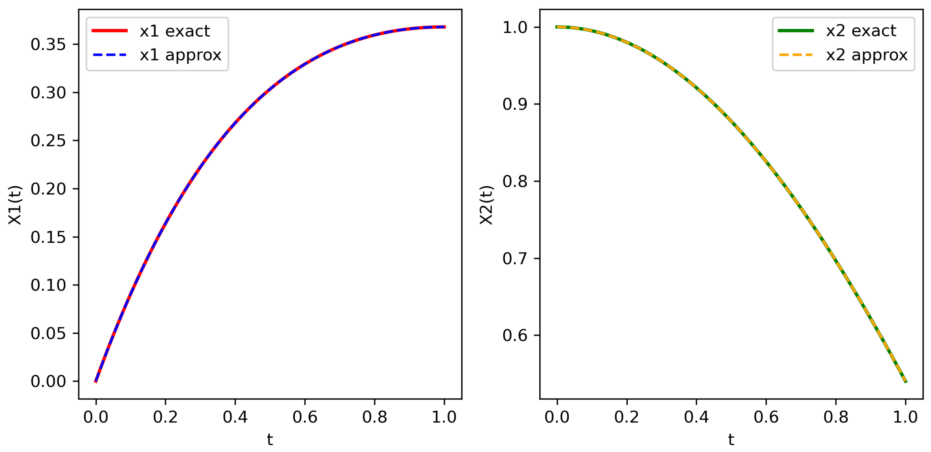
RMSE	0.3202327707	0.1974042058	0.0019485851	0.0012139441

and Figure 1.

In Table 1 and below, we employ the following notations: N is the degree of the approximating polynomial from formula (26), Err $x_i\left(t\right),i=1,2,$ is the difference between the exact and approximate solutions in the corresponding norms.

Table 2. Condition numbers of matrix $\mathbf{A}$ for Example 7. Values are rounded to three significant digits.

Variant	Condition Number
	$\mathit{N}=\mathbf{8}$	$\mathit{N}=\mathbf{12}$
1	$2.614\times {10}^{13}$	$3.206\times {10}^{18}$
2	$5.622\times {10}^{13}$	$1.628\times {10}^{19}$
3	$4.943\times {10}^{13}$	$9.874\times {10}^{18}$
4	$9.167\times {10}^{13}$	$8.445\times {10}^{19}$

provides condition numbers for matrix $\mathbf{A}$ from formula (28) for Example 7, which illustrates how singular points (Variants 2 and 3) and higher index (Variant 4) affect the quality of the solution. The condition numbers were computed using the NumPy library in Python, and the results were evaluated with respect to the 2-norm.

In the above examples, we considered cases where the sought solutions are relatively simple functions, such as exponential or trigonometric functions with moderate oscillations. However, when the parameters involved vary significantly, leading to solutions with very large exponents or highly complex oscillations, the approximation of such functions becomes challenging. In these situations, the approximation error can increase rapidly and substantially, even for small changes in the input parameters.

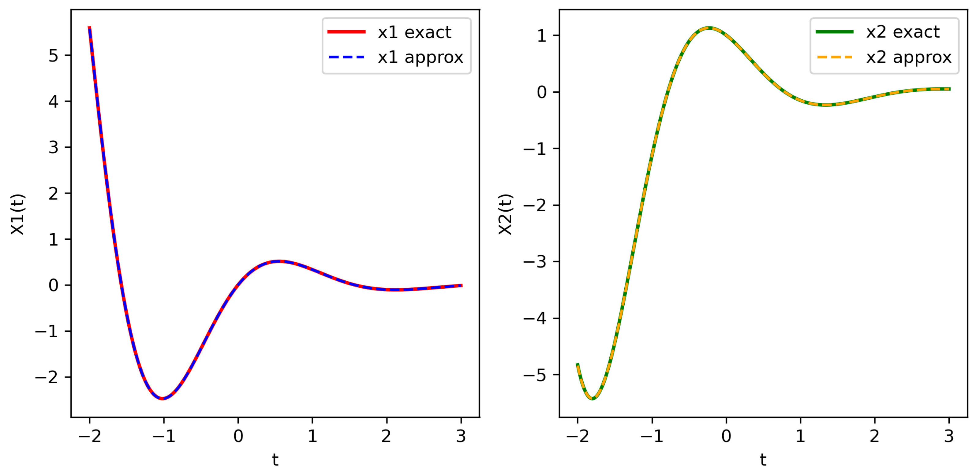
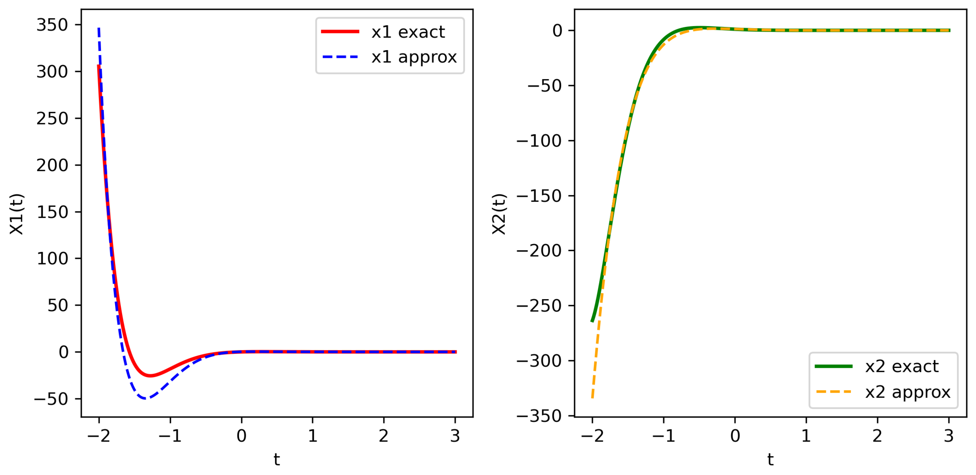
For instance, when increasing the parameter $c=3$ in Example 7—Variant 1, the exact solution exhibits exponential behavior, resulting in values of large magnitude over the interval $\left[\alpha ,\beta \right]$, which are difficult to approximate accurately. The results presented in

Table 3. Error comparison between the exact solutions and the approximate solutions obtained by the LSM method using a polynomial of degree 12 for Example 7—Variant 1 with $a=2$ and $c=3$.

	Err x1(t)	Err x2(t)
R2	0.9531691116	0.9848603552
MAE	4.9203841607	2.1378850533
MSE	103.8837244214	58.4761322750
RMSE	10.1923365536	7.6469688292

and Figure 2 show that the approximation errors increase sharply under these conditions.

Therefore, it is essential to carefully examine the ill-conditioning of the problem under study and apply suitable techniques to mitigate this issue. For example, to reduce the ill-conditioning in Example 7—Variant 1, before applying the LSM, we can perform a substitution of variable

$$x\left(t\right)=e^{-ct}u\left(t\right),$$

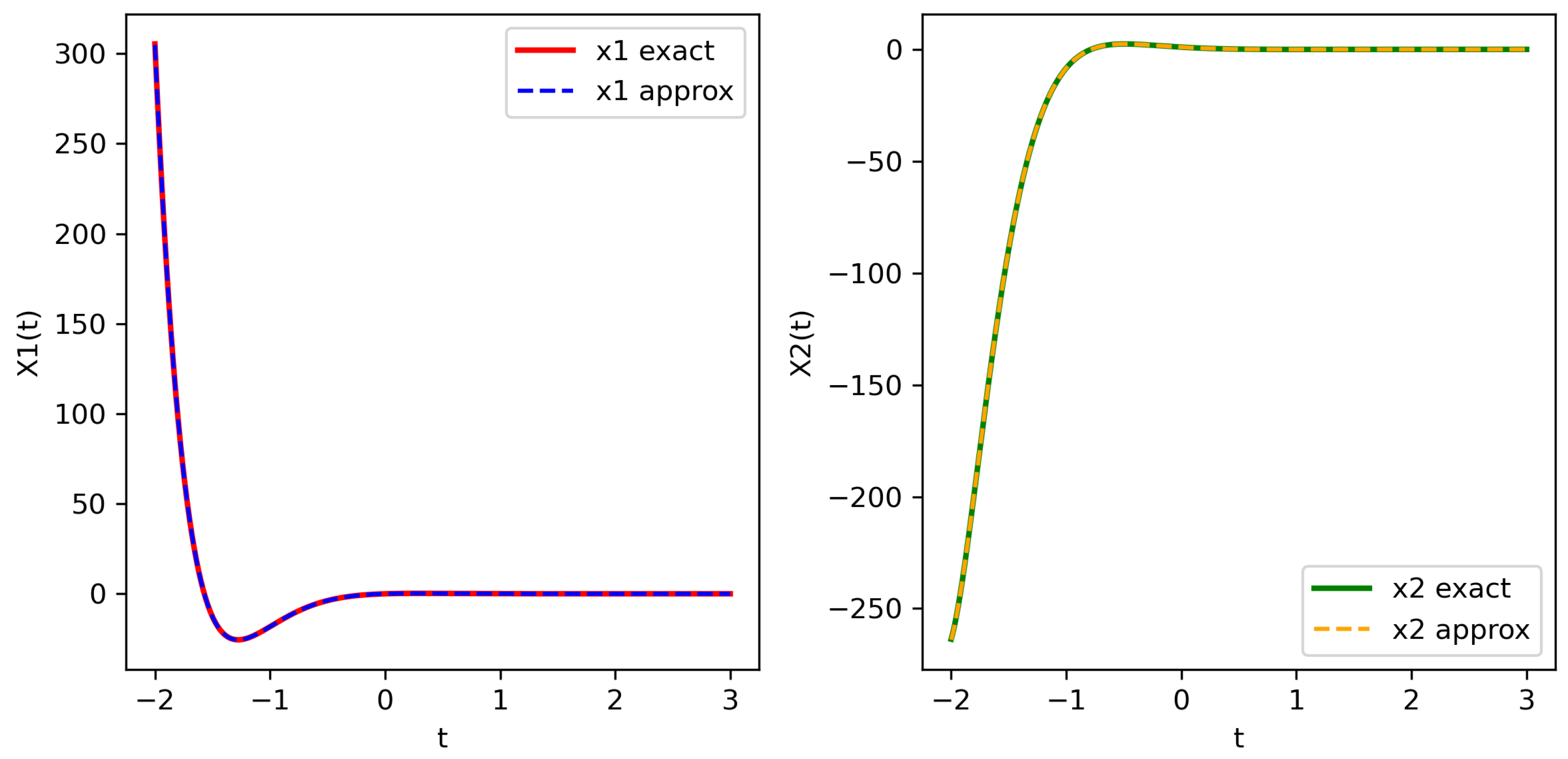
which eliminates the exponential growth component in the equation. Then, the LSM is applied to determine the solution $u\left(t\right)$, and once $u\left(t\right)$ is obtained, the desired solution $x\left(t\right)$ can be recovered. The results shown in

Table 4. Error comparison between the exact solutions and the approximate solutions obtained by the LSM method using a polynomial of degree 12 for Example 7—Variant 1 with $a=2$ and $c=3$ after applying the variable transformation technique.

	Err x1(t)	Err x2(t)
R2	0.9999990294	0.9999998608
MAE	0.0078367521	0.0043363098
MSE	0.0017446990	0.0004547880
RMSE	0.0417695942	0.0213257601

and Figure 3 demonstrate that the errors are significantly reduced after applying this transformation.

Example 8.

The following system was successfully solved by the collocation method in [11]:

$$({\mathrm{\Lambda }}_0+\mathcal{V})x=\left(\begin{array}{cc}1& 0\\ 0& 0\end{array}\right)x\left(t\right)+\underset{\alpha }{\overset{t}{\int }}\left(\begin{array}{cc}(t-s)& e^{(t-s)}\\ e^{(2t-s)}& 0\end{array}\right)x\left(s\right)ds=\varphi \left(t\right),t\in T=[0,1],$$

where $x\left(t\right)={\left(\begin{array}{cc}rt{e}^{ct}& cos\left(t\right)\end{array}\right)}^{\top }$. We choose $\varphi \left(t\right)=\left(\begin{array}{c}rt{e}^{ct}+r(-2e^{ct}+ct{e}^{ct}+2+ct)/c^3-1/2cos\left(t\right)+1/2sin\left(t\right)+1/2e^t\\ r(-e^{t+ct}t+e^{t+ct}ct-e^{t+ct}+e^{2t})/{(-1+c)}^2\end{array}\right)$. Eventually, we obtain

$${\mathrm{\Omega }}_2=\left(\begin{array}{cc}1& 0\\ 0& d/dt\end{array}\right)\left(\begin{array}{cc}1& 0\\ -e^t& 1\end{array}\right)\left(\begin{array}{cc}1& 0\\ 0& d/dt\end{array}\right),\det \tilde{A}\left(t\right)=\left(\begin{array}{cc}1& 0\\ e^t& e^t\end{array}\right)=e^t.$$

Table 5. Error comparison between the exact and approximate solutions using polynomials of degree 4 and 8 for Example 8.

	$\mathit{N}=4$		$\mathit{N}=8$
	Err x1(t)	Err x2(t)	Err x1(t)	Err x2(t)
R2	0.9999998530	0.9999595814	0.9999999999	0.9999999999
MAE	$2.89849\times {10}^{-5}$	0.0005036297	$2.90920\times {10}^{-9}$	$8.73211\times {10}^{-8}$
MSE	$1.62710\times {10}^{-9}$	$7.76174\times {10}^{-7}$	$1.62969\times {10}^{-17}$	$2.86561\times {10}^{-14}$
RMSE	$4.03373\times {10}^{-5}$	0.0008810072	$4.03694\times {10}^{-9}$	$1.69281\times {10}^{-7}$

presents the error comparison between the exact and approximate solutions obtained by the LSM for Example 8 with $r=1$ and $c=-1$, where the degrees of the approximating polynomials are 4 and 8. The results show that in this case, the LSM is just as successful as the collocation method proposed in [11].

Figure 4 illustrates the direct comparison between the exact and approximate solutions obtained by the LSM for Example 8 with $r=1$ and $c=-1$, where the degree of the approximating polynomials is 8.

Comparison with the conventional right rectangle method (21) reveals the superiority of the LSM approach. We implement an algorithm based on formula (21) in Python. The computations produce the following results: the right rectangle method converges with a first-order accuracy only for Variant 1 and diverges or is inapplicable for other variants, while the LSM provides stable and accurate solutions across all test cases. This robustness makes the LSM particularly valuable for practical applications where singular points may be present.

The proposed LSM has several limitations. First, like any spectral method, it is effective for solutions that are smooth functions. Second, for solutions with rapid exponential growth (as in Example 7 with $c=3$), the direct application of the method leads to extreme ill-conditioning.

The main computational costs in solving system (28) consist of: (1) Filling the matrix A of size $n(N+1)\times n(N+1)$, which requires computing $O\left({\left(nN\right)}^2\right)$ integrals of function products. (2) Solving the resulting dense system of linear equations, which has a complexity of $O\left({\left(nN\right)}^3\right)$. (3) The condition number grows with N and can affect numerical stability for very high degrees for polynomials of higher degrees. Compared to the step-by-step finite difference methods, which have linear complexity $O\left(N\right)$, the LSM is less efficient for very large N. In the case of IAEs with singular points, where difference methods may not converge, the complexity comparison is not entirely correct.

The stability of the LSM is ensured by its global nature. While step-by-step methods (finite difference and collocation) may diverge when a grid node coincides with a singular point or its neighborhood (significantly smaller than the step size), the LSM seeks an approximation over the entire interval. This typically results in limited, though reduced, accuracy in the vicinity of the singular point. Additionally, at this stage of research, we are unable to describe the behavior of the solution neat singular points as it is done, for example, for scalar cases in [34,35].

7. Discussion and Conclusions

The main scientific contributions of this work are as follows:

1.

Formalization of the concept of a singular point for IAEs within the framework of the operator approach using a left regularizing operator (LRO). This allows for a unified interpretation of points’ singularity, where the classical solvability theory breaks down.

2.

Development and theoretical justification of a numerical scheme based on the least squares method (LSM) in Sobolev spaces for solving IAEs with singular points. Unlike step-by-step methods (finite-difference, collocation), the proposed method seeks a solution globally over the entire interval, thus eliminating problems that arise when grid nodes coincide with singular points.

3.

Theoretical analysis of the convergence of the proposed LSM approach (Theorem 4, Lemma 6), establishing a connection between the smoothness of the solution and the decay rate of the residual functional.

4.

A numerical investigation was conducted using test examples. The stability of the LSM in the presence of singular points is demonstrated.

5.

As a result of analyzing the numerical experiments, a hypothesis has emerged: the LSM, when using the residual in the $L_2$ norm, also guarantees the convergence of the approximations to the solution of the original problem. Finding a proof of this fact constitutes the next stage of the research.

These results develop and supplement existing works on collocation and finite-difference methods for IAEs, for the first time proposing a unified stable approach for problems with degenerate points, based on a variational formulation.

Future work suggests several promising research directions. These include applying the method to problems with non-smooth solutions arising from singular points, investigating the use of orthogonal basis functions to improve the conditioning of the numerical scheme, developing refined analytical tools to characterize solution behavior near singularities, and conducting comparative studies with specialized techniques such as collocation on graded meshes.