Article

On Minimum Bregman Divergence Inference

by
Soumik Purkayastha
1,2,* and
Ayanendranath Basu
3
1
Department of Biostatistics and Health Data Science, University of Pittsburgh, Pittsburgh, PA 15261, USA
2
Center for Healthcare Evaluation, Research, and Promotion, VA Pittsburgh Health System, Pittsburgh, PA 15261, USA
3
Interdisciplinary Statistical Research Unit, Indian Statistical Institute, Kolkata 700108, West Bengal, India
*
Author to whom correspondence should be addressed.
Mathematics 2026, 14(4), 670; https://doi.org/10.3390/math14040670
Submission received: 14 January 2026 / Revised: 8 February 2026 / Accepted: 9 February 2026 / Published: 13 February 2026

Abstract

The density power divergence (DPD) is a well-studied member of the Bregman divergence family and forms the basis of widely used minimum divergence estimators that balance efficiency and robustness. In this paper, we introduce and study a new sub-class of Bregman divergences, termed the exponentially weighted divergence (EWD), designed to generate competitive and practically interpretable inference procedures. The EWD is constructed so that its associated weight function remains bounded within the interval [ 0 ,   1 ] , which facilitates a transparent interpretation of robustness through controlled downweighting of low-density observations and avoids excessive influence from high-density points. We develop minimum EWD estimators (MEWDEs) within a general framework accommodating independent but non-homogeneous data, thereby extending classical minimum divergence theory beyond the i.i.d. setting. Under standard regularity conditions, we establish Fisher consistency and asymptotic normality, and we analyze robustness properties through influence function calculations. The EWD framework is further extended to parametric hypothesis testing, for which we derive the asymptotic null distribution of a Bregman divergence-based test statistic. Extensive simulation studies and real-data applications demonstrate that the proposed estimators perform comparably to, and often more robustly than, existing DPD-based procedures, particularly under moderate to heavy contamination, while retaining high efficiency under clean data. Overall, the EWD provides a tractable and interpretable alternative within the Bregman divergence class for robust parametric estimation and testing.

1. Introduction

  Density-based minimum divergence methods are popular tools in statistical inference. In parametric estimation, this amounts to choosing the model density closest (in terms of the selected divergence) to the empirical data density. This approach often combines strong robustness properties with high asymptotic efficiency. An important class of density-based divergences is the class of ϕ divergences (see [1]). Under standard regularity conditions, all minimum ϕ divergence estimators have full asymptotic efficiency at the model [2]; many also have attractive robustness properties. The seminal Hellinger distance study of [3] appears to be the first which demonstrated that strong robustness properties may be achieved simultaneously with full asymptotic efficiency. Later, the same has been demonstrated with respect to much of the ϕ divergence class (see, e.g., [4]). The usefulness of the corresponding procedures in providing robust alternatives to the likelihood ratio test has also been explored in the literature [2,4,5]. The approach has been further refined and extended in many directions by later authors. On the whole, the utility of the minimum divergence procedures based on ϕ divergences is well established in the literature.
One major criticism of this inference procedure is that it inevitably involves the use of some form of non-parametric smoothing (such as kernel density estimation) to produce a continuous estimate of the true density. This can throw up several potential difficulties including the problematic bandwidth selection issue and the slow convergence of the of kernel density estimator to the “truth” (particularly for high dimensional data). The theoretical derivations are also harder. Development of methods which eliminate these difficulties may be worthwhile even if that involves a marginal loss in asymptotic efficiency.
An alternative class of minimum divergence estimators which avoids non-parametric smoothing in the construction of the empirical divergence is the class of minimum Bregman divergence estimators. An important example is the family of density power divergences (henceforth DPD( α ), where α is the tuning parameter); the corresponding minimum density power divergence estimators (henceforth MDPDE( α )) have been shown to combine strong robustness properties with high asymptotic efficiency (see [6]). Divergences within the Bregman class have been called decomposable divergences by [7] and non-kernel divergences by [8]. These divergences have simple estimating equations and much of their asymptotic properties can be obtained from the M-estimation theory. The Kullback–Leibler divergence, which is a decomposable divergence, is the only common member between the ϕ divergence and the Bregman divergence classes.
The application of Bregman divergences continues to expand rapidly into complex domains. Recent studies have successfully adapted these measures for multivariate time series analysis, including change-point and anomaly detection [9,10]. In the realm of geometric data analysis, variants like the Total Bregman Divergence have been applied to K-Means clustering for point cloud denoising [11]. On the theoretical front, new bounds on excess minimum risk have been established for generalized divergence measures [12], while recent work in econometrics has utilized these concepts for the robust learning of tail dependence [13].
In the context of density-based minimum divergence estimation, we have several “good” choices available. To justify the development of another family of estimators, one must demonstrate that the new estimators are competitive, if not better than the existing standard. Within the class of minimum divergence estimators which do not require any nonparametric smoothing, the MDPDE( α ) is the current standard. In this paper, we will develop a family of divergences yielding minimum divergence estimators which satisfy this requirement; at the least, this family provides a highly competitive standard. Our proposed class of divergences will be called the exponentially weighted divergence family, indexed by a tuning parameter β (henceforth referred to as EWD( β )). The corresponding minimum divergence estimator will be denoted by MEWDE( β ). This divergence will also be useful in the field of hypothesis testing. Although the likelihood ratio test has several asymptotic optimality properties at the model, it is also known to have very poor robustness properties. Many density-based minimum distance procedures yield robust tests of hypothesis with high efficiency, e.g., Refs. [14,15,16]. Some of these papers address the general problem of parametric hypothesis testing based on the density power divergence. The present work considers this problem in the context of a general Bregman divergence, with special emphasis on our proposed EWD( β ) class. To summarize, the main results of this paper are fourfold:
  • We introduce the exponentially weighted divergence (EWD), a novel sub-class of Bregman divergences. Unlike the popular density power divergence (DPD), the EWD is constructed to ensure the associated weight function remains bounded within the [ 0 ,   1 ] interval.
  • We derive the asymptotic properties (consistency and normality) of the minimum EWD estimator (MEWDE) for independent non-homogeneous data.
  • We extend the framework to parametric hypothesis testing and derive the asymptotic null distribution of the test statistic.
  • We evaluate the method through simulations and real-data applications, comparing its performance against the density power divergence (DPD) and classical robust estimators.
It is instructive to situate the proposed EWD within the broader landscape of robust statistics, while classical robust methods such as M-estimators, Least Median of Squares (LMS), and MM-estimators focus on minimizing residual functions, the proposed EWD approach belongs to the class of minimum divergence estimators. This distinction is crucial: by minimizing a probability distance, the MEWDE naturally achieves high asymptotic efficiency at the model—a property that often requires complex, multi-step procedures in standard high-breakdown regression (e.g., MM-estimation). Furthermore, within the divergence framework, it is important to distinguish the EWD from the class of ϕ -divergences [1], which includes the Hellinger distance and Pearson’s χ 2 ; while ϕ -divergences offer strong geometric properties, they often result in estimating equations that are computationally intensive or require non-parametric density estimation components. In contrast, the EWD belongs to the Bregman divergence class. This ensures that the resulting estimators share the tractable, decomposable structure of the Maximum Likelihood Estimator (MLE) and can be easily implemented for any member of the exponential family. The EWD thus combines the desirable bounded-influence properties often sought in ϕ -divergence inference with the computational simplicity of the Bregman framework.
The rest of this paper is organized as follows. Section 2 introduces the general framework of minimum Bregman divergence estimation for independent non-homogeneous observations and defines our proposed sub-class, the EWD family. Section 3 establishes the theoretical properties of the estimator, including Fisher consistency and asymptotic normality, and analyzes its robustness via the influence function. Section 4 presents extensive simulation studies comparing the finite-sample performance of the proposed method against existing standards and discusses a data-driven strategy for selecting the optimal tuning parameter controlling trade-off between efficiency and robustness of MEWDEs. Section 5 demonstrates the practical utility of the estimator through several real-data examples, ranging from univariate problems to multiple linear regression. Section 6 extends the framework to robust hypothesis testing and derives the asymptotic null distribution of the proposed test statistic. Finally, Section 7 offers concluding remarks, while proofs and additional regression examples are provided in the Appendices.

2. The Bregman Divergence

2.1. Introduction to Minimum Bregman Divergence Estimation

The Bregman divergence between two densities g and f with common support X is defined as
D B ( g , f ) = X [ B ( g ( x ) ) B ( f ( x ) ) ( g ( x ) f ( x ) ) B ( f ( x ) ) ] d x ,
where B : R R is a strictly convex function and B ( · ) is the derivative of B with respect to its argument. The integral in (1) is defined over the support X of the densities f and g. The strict convexity of B assures that the measure D B ( g , f ) is non-negative, and equals zero if and only if the arguments are identically equal. Ref. [17] discusses this and other measures in greater detail. We note that the convex functions B ( y ) and B * ( y ) = B ( y ) + a y + c generate identical divergences in Equation (1) for a , c R . In this section, we discuss minimum Bregman divergence inference in case of data that are independent, but not necessarily identically distributed. The i.i.d. data case emerges as a special case of this setup.
We assume that the data X 1 , , X n are independent. For i = 1 , 2 , , n we have X i g i , where g i are possibly different densities with respect to some common dominating measure. We model g i by the family F i , θ = { f i , θ θ Ω R s } for each i = 1 , 2 , , n , where s denotes the dimension of the parameter vector θ . An estimate of the Bregman divergence between the density g i and the associated model density f i , θ ( F i , θ ) is given by D B ( g ^ i , f i , θ ) , where g ^ i is a non-parametric density estimate of g i .
Since our aim is to reach some “common” value of θ (if it exists) which can be used to model each g i individually, it is intuitive to minimize the average divergence between the data points and the models, given by H n ( θ ) = n 1 i = 1 n D B ( g ^ i , f i , θ ) with respect to θ . In the presence of only one data point X i from density g i , the best density estimate of g i is the (degenerate) density which puts the entire mass on the observed value of X i and this yields the objective function (ignoring the terms independent of θ ) given by
H n ( θ ) = 1 n i = 1 n f i , θ ( x ) B ( f i , θ ( x ) ) B ( f i , θ ( x ) ) d x B ( f i , θ ( X i ) ) = 1 n i = 1 n V i , θ ( X i ) .
Let θ represent the gradient with respect to θ . Considering partial derivatives of the objective function in Equation (2), we arrive at the estimating equation
i = 1 n u i , θ ( X i ) w ( f i , θ ( X i ) ) u i , θ ( x ) w ( f i , θ ( x ) ) f i , θ ( x ) d x = 0 ,
where u i ( x ) = θ log ( f i , θ ( x ) ) is the likelihood score function of the density f i , θ ( x ) used to model the i-th data point, and w ( t ) = B ( t ) × t . If the data were i.i.d. with common density g, we would choose a common model density f θ for modeling and inference. Consequently, Equation (3) would yield
i = 1 n u θ ( X i ) w ( f θ ( X i ) ) u θ ( x ) w ( f θ ( x ) ) f θ ( x ) d x = 0 ,
where u θ ( x ) = θ log ( f θ ( x ) ) is the likelihood score function of the model density f θ ( x ) . Equation (3) is a generalization of weighted likelihood estimating equation for the case of independent and non-homogeneous data.

2.2. The Exponentially Weighted Divergence

To develop new estimation procedures based on Bregman divergences, one can either (a) start with a specific convex function B as given in Equation (2) and construct a weighted likelihood equation, or (b) begin with a suitable robust weight representation as in Equation (3) and backtrack to recover the corresponding convex function B. We take the latter approach.
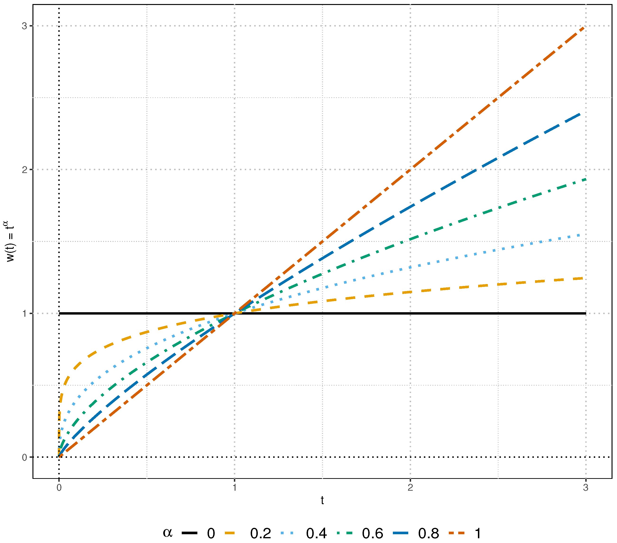
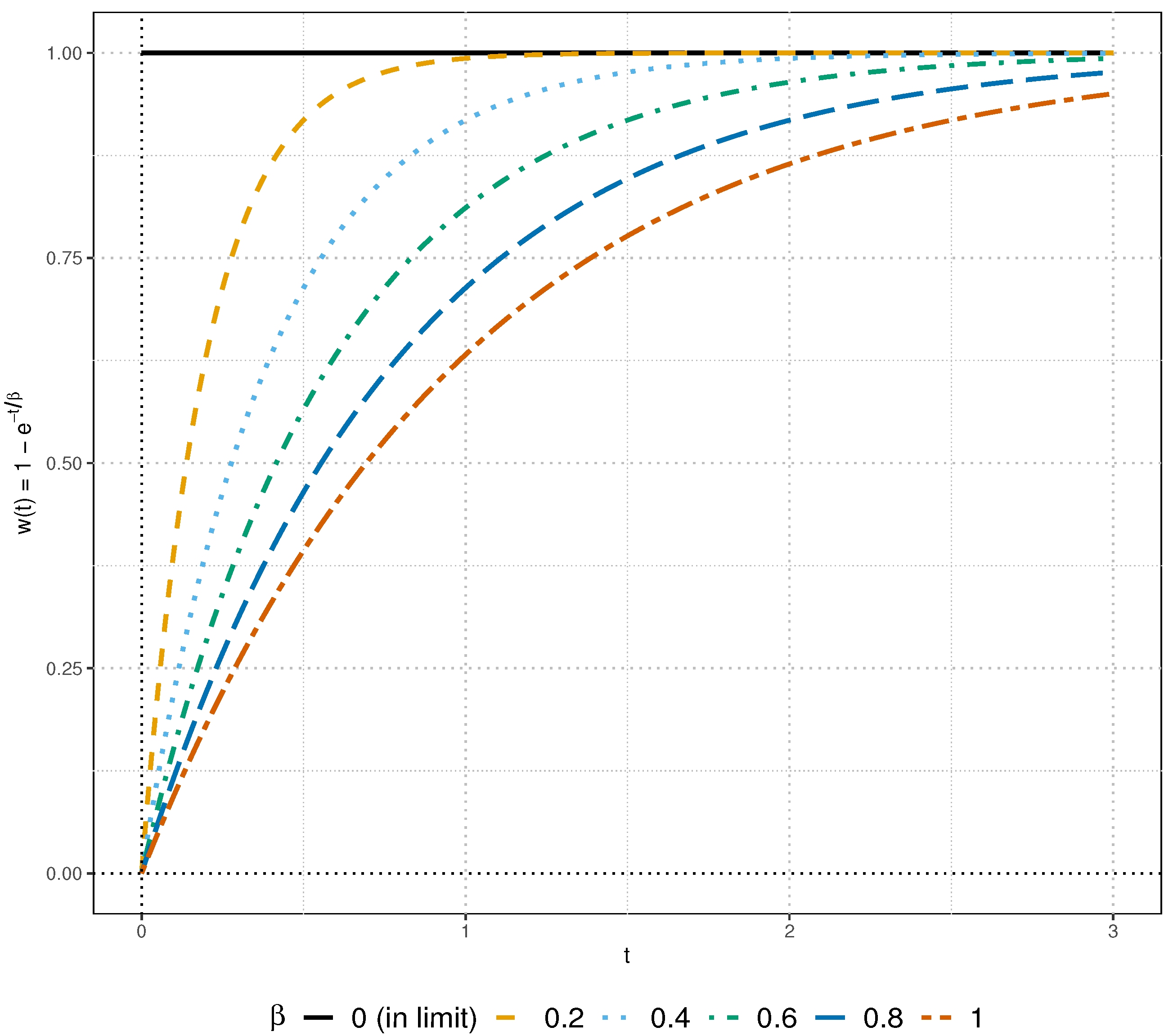
Philosophically, our treatment of outliers is probabilistic; an outlying point is one which has a small probability of occurrence under the model f θ F θ . We downweight those observations in the estimating equation for which the value of f θ ( x ) is small. We plot the weight functions for some members of the DPD( α ) family at different values of α in Figure 1. We note that the strength of downweighting increases with increasing α . For f θ ( x ) > 1 , these weights grow unboundedly for all α > 0 as the argument increases.
As an alternative, we propose a new class of divergences based on a different choice of the weight function given by (depending on a non-negative index β )
w β ( t ) = 1 exp ( t / β ) if β > 0 , 1 if β = 0 .
These weights smoothly drop to zero for decreasing values of the pdf f θ ( x ) for β > 0 . Unlike the DPD( α ) weights, they are bounded above by 1. We plot the weight functions given by Equation (4) for specific values of β in Figure 2.
The likelihood equation may be recovered at β = 0 , where, to avoid the complications of division by zero, the weights have been defined by the corresponding limiting case as β 0 . Using the relation w ( t ) = B ( t ) × t , we recover the associated B function
B β ( x ) = x 2 β n = 0 ( x / β ) n ( n + 2 ) ! ( n + 1 ) .
In the appendix, we show that this can be further simplified to
B β ( x ) = x + γ x + β β exp ( x / β ) + x Γ ( 0 , x / β ) + x log ( x / β ) ,
where γ is the Euler–Mascheroni constant and Γ ( α , β ) is the incomplete Gamma integral. We can equivalently consider the following simplified form of the defining function:
B β * ( x ) = β exp ( x / β ) + x Γ ( 0 , x / β ) + x log ( x / β ) .
The associated Bregman divergence (which we will refer to as the exponentially weighted divergence EWD( β ) ) has the form
1 n i = 1 n f i , θ ( x ) B ( f i , θ ( x ) ) B ( f i , θ ( x ) ) d x B ( f i , θ ( X i ) ) ,
where B = B β * is as in Equation (5). The MEWDE( β ) solves the estimating equation
i = 1 n u i , θ ( X i ) 1 exp f i , θ ( X i ) / β u i , θ ( x ) 1 exp f i , θ ( x ) / β f i , θ ( x ) d x = 0 .
Remark 1.
We do not claim that the exponential weight function defining the EWD is unique among bounded weighting schemes within the Bregman divergence class. Indeed, infinitely many bounded weight functions could be constructed that yield valid Bregman divergences. The contribution of the present work is not to establish a universal optimality or uniqueness result, but rather to identify a particularly tractable and interpretable member of this class. The exponential form w ( t ) = 1 exp ( t / β ) offers three practical advantages simultaneously: (i) weights are strictly bounded in w [ 0 , 1 ] , preventing inlier super-weighting; (ii) the resulting divergence retains the decomposable structure required for fast M-estimation; and (iii) the tuning parameter β admits a transparent probabilistic interpretation in terms of downweighting low-likelihood observations. These properties together motivate the EWD as a natural and practically appealing alternative to existing Bregman divergences such as the DPD.
Remark 2.
We note that the standard Maximum Likelihood Estimator (MLE) corresponds to the limiting case of the proposed EWD family. As the tuning parameter β , the weight function converges to unity ( w ( f ( x ) ) 1 ) for all x. Consequently, the estimating Equation (3) reduces to the classical likelihood score equation. This theoretical connection justifies the use of the MLE as the baseline for efficiency comparisons ( β ) throughout the simulation and application sections.

3. Properties

3.1. Fisher Consistency of Minimum Bregman Divergence Estimators

We consider independent data X 1 , , X n with X i g i , where g i are (possibly) different densities with respect to some common dominating measure. Let G i be the distribution function associated with g i for i = 1 , 2 , , n . The minimum Bregman divergence functional T B ( G 1 , G 2 , , G n ) for non-homogeneous observations is given by the relation T B ( G 1 , G 2 , , G n ) = argmin θ Ω H n * ( θ ) , where H n * ( θ ) = 1 n i = 1 n D B ( g i , f i , θ ) is the theoretical version of the expression as defined by Equation (2). As the Bregman divergence so defined is a genuine divergence in the sense that it is non-negative and attains its minimum if and only if each data generating distribution G i equals the model counterpart F i , θ , the functional T is Fisher consistent in the sense T ( F 1 , θ , F 2 , θ , , F n , θ ) = θ .

3.2. Asymptotic Properties

We derive the asymptotic distribution of the minimum Bregman divergence estimator θ ^ n defined by the relation θ ^ n = argmin θ Ω H n ( θ ) , provided such a minimum exists, where H n ( θ ) is as defined in Equation (2). In particular the presented results hold for MEWDE( β ).
We assume that the data are generated from the setup described in Section 3.1. We model g i by the parametric family F i , θ = { f i , θ : θ Ω , Ω R s } for each i = 1 , 2 , , n . We also assume that there exists a best fitting value of θ which is independent of the index i of the different densities and lets us denote it by θ g . It is important to note that this assumption is satisfied if all the true densities g i belong to the model family so that g i = f i , θ for some common θ = θ g . The minimum Bregman divergence estimating equation is given by Equation (3), which is solved by the minimizer of H n ( θ ) as defined in Equation (2). We now define, for i = 1 , 2 ,
H ( i ) ( θ ) = f i , θ ( x ) B ( f i , θ ( x ) ) B ( f i , θ ( x ) ) B ( f i , θ ( x ) ) g i ( x ) d x ,
so that for the best fitting parameter θ g , we have θ H ( i ) ( θ g ) = 0 , for i = 1 , 2 , We also define, for each i = 1 , 2 , , the s × s matrix J ( i ) with ( k , l ) -th entry given by
J k l ( i ) = E g i [ k l V i , θ ( X i ) ] ,
where V i , θ ( X i ) is as defined in Equation (2), k l V i , θ ( X i ) = 2 V i , θ ( X i ) θ k θ l is the ( k , l ) -th component of θ V i , θ ( X i ) , E g i [ · ] denotes expectation under the distribution specified by g i , and θ i denotes the i-th component of θ . We also define
Ψ n = 1 n i = 1 n J ( i ) ,
and the matrix
Ω n = 1 n i = 1 n V g i [ θ V i , θ ( X i ) ] ,
where V g i denotes taking variance under the distribution specified by g i . The matrix defined in Equation (9) has the following expression:
J ( i ) = u i , θ g ( x ) u i , θ g T ( x ) w ( f i , θ g ( x ) ) f i , θ g ( x ) d x + θ u i , θ g ( x ) + u i , θ g ( x ) u i , θ g T ( x ) h i ( x ) f i , θ g ( x ) g i ( x ) w ( f i , θ g ( x ) ) d x ,
where w ( t ) = B ( t ) × t , w is the derivative of w w.r.t. its argument and
h i ( t ) = w ( f i , θ ( t ) ) f i , θ ( t ) / w ( f i , θ ( t ) ) .
Similarly, the matrix defined in Equation (11) has the expression
Ω n = 1 n i = 1 n u i , θ g ( x ) u i , θ g T ( x ) w 2 ( f i , θ g ( x ) ) g i ( x ) d x ξ i ξ i T ,
where ξ i = u i , θ g ( x ) w ( f i , θ g ( x ) ) g i ( x ) d x . We will make the following assumptions to establish the asymptotic properties of the minimum Bregman divergence estimators. These are in the spirit of [6], with appropriate modifications to cover the general independent but non-homogeneous data case.
Assumption 1.
The support χ = { x : f i , θ ( x ) > 0 } is independent of i and θ for all i; the true densities g i are also supported on χ for all i.
Assumption 2.
There is an open subset ω of the parameter space Ω, containing the best fitting parameter θ g such that for almost all x χ , and all θ Ω , all i = 1 , 2 , , the density f i , θ ( x ) is thrice differentiable with respect to θ and the third partial derivatives are continuous with respect to θ.
Assumption 3.
For i = 1 , , n , both [ f i , θ ( x ) B ( f i , θ ( x ) ) B ( f i , θ ( x ) ) ] d x and B ( f i , θ ( x ) ) g i ( x ) d x can be differentiated thrice with respect to θ, and the derivatives can be taken under the integral sign.
Assumption 4.
For each i = 1 , 2 , the matrices J ( i ) are positive definite and λ 0 = inf n [ min   eigenvalue   of   Ψ n ] is positive.
Assumption 5.
There exists a function M j k l ( i ) ( x ) such that j k l V i , θ ( x ) M j k l ( i ) ( x ) θ Ω and i = 1 , 2 , where n 1 i = 1 n E g i [ M j k l ( i ) ( X i ) ] = O ( 1 ) j , k , l .
Assumption 6.
For all j , k we have
lim N sup n { 1 n i = 1 n E g i ( j V i , θ ( X i ) I ( j V i , θ ( X i ) > N ) ) } = 0 . lim N sup n { 1 n i = 1 n E g i j k V i , θ ( X i ) E g i ( j k V i , θ ( X i ) ) × I j k V i , θ ( X i ) E g i ( j k V i , θ ( X i ) ) > N ) } = 0 .
where I ( A ) denotes the indicator variable associated with the event A.
Assumption 7.
For all ϵ > 0 , we have
lim n i = 1 n E g i Ω n 1 / 2 θ V i , θ ( X i ) 2 I Ω n 1 / 2 θ V i , θ ( X i ) > ϵ n = 0 .
Theorem 1.
Under Assumptions 1–7, the following results hold.
1. 
There exists a consistent sequence θ ^ n of roots satisfying the minimum Bregman divergence estimating equation given by Equation (3).
2. 
The asymptotic distribution of Ω n 1 / 2 Ψ n [ n ( θ ^ n θ g ) ] is s-dimensional normal with mean vector 0 and covariance I s , the s-dimensional identity matrix.
The proof is provided in Appendix D.
Remark 3.
Setting f i = f i , we get the corresponding asymptotic properties of the minimum Bregman divergence estimator for i.i.d. case as given in Basu et al. [6]. In particular, choosing B ( x ) = x 1 + α / α , we recover the asymptotic distribution of MDPDE(α). Assumptions 1–5 are similar to those given by Basu et al. [6], while Assumptions 6 and 7 are automatically satisfied by the dominated convergence theorem for i.i.d. data.
Remark 4.
Intuition regarding Assumptions 1–7: Conditions (1)–(4) are standard regularity assumptions required for the consistency and asymptotic normality of M-estimators, ensuring model identifiability, differentiability of the log-likelihood, and non-singularity of the Fisher Information Matrix. Conditions (5)–(7) are necessary to extend these results from the i.i.d. setting to the case of independent non-homogeneous observations. Specifically, (5) ensures the uniform boundedness of the third derivatives, allowing for valid Taylor expansions across varying densities g i ; (6) provides the uniform integrability required for the Law of Large Numbers to apply to the score and Hessian matrices; and (7) is the standard Lindeberg–Feller condition, which ensures that the sum of independent (but non-identical) score functions converges to a normal distribution by preventing any single observation from dominating the asymptotic variance. Ideally, the bounded nature of the EWD weight function ( w [ 0 , 1 ] ) facilitates the satisfaction of these moment conditions compared to unbounded influence functions. These conditions are widely satisfied by standard exponential families (e.g., normal, Poisson) under compact parameter spaces

3.3. Influence Function Analysis

Let G i ( g i ) be the true distribution (density) for Y i , i = 1 , 2 , , n and T B ( G 1 , G 2 , , G n ) be the minimum Bregman divergence functional obtained, under appropriate regularity conditions, as the solution of the system given by Equation (3). To derive the influence function of the minimum Bregman divergence estimator in the context of non-homogeneous data, we consider the set of contaminated distributions G i , ϵ = ( 1 ϵ ) G i + ϵ Δ ( t i ) , where ϵ ( 0 , 1 ) represents the contamination proportion and Δ ( t i ) denotes the Dirac measure, representing the degenerate distribution at the point of contamination t i ( i = 1 , 2 , , n ). The associated contaminated density is given by g i , ϵ . Let θ 0 = T B ( G 1 , G 2 , , G n ) and let θ ϵ i = T B ( G 1 , G 2 , , G i 1 , G i , ϵ , G i + 1 , , G n ) be the minimum Bregman divergence functional with contamination only in the i-th direction. Substituting θ ϵ i and g i , ϵ in the estimating Equation (3), differentiating with respect to ϵ and evaluating the derivative at ϵ = 0 , we obtain the influence function of the functional which considers contamination only along the i-th direction to be
I F i ( t i , T B , G 1 , G 2 , , G n ) = Ψ n 1 n u i , θ ( t i ) w ( f i , θ ( t i ) ) ξ i ,
where Ψ n is as defined in Equation (10), w ( t ) = B ( t ) × t and ξ i = u i , θ ( x ) w ( f i , θ ( x ) ) g i ( x ) d x . Letting θ ϵ = T B ( G 1 , ϵ , G 2 , ϵ , , G n , ϵ ) and proceeding similarly, we obtain the influence function with contamination at all the data points as
I F ( t 1 , , t n , T B , G 1 , , G n ) = Ψ n 1 n i = 1 n u i , θ ( t i ) w ( f i , θ ( t i ) ) ξ i .
In particular, letting t i = t , G i = G and f i = f , i , we get back the influence function of the minimum Bregman divergence estimator for the i.i.d. case. In particular, for the MEWDE( β ), the influence function reduces to
I F ( t , T β , G ) = J 1 u θ ( t ) 1 exp ( f θ ( t ) / β ) ξ ,
where
J = u θ ( x ) u θ T ( x ) [ 1 exp ( f θ ( x ) / β ) ] f θ ( x ) d x , ξ = u θ ( x ) [ 1 exp ( f θ ( x ) / β ) ] f θ ( x ) d x .
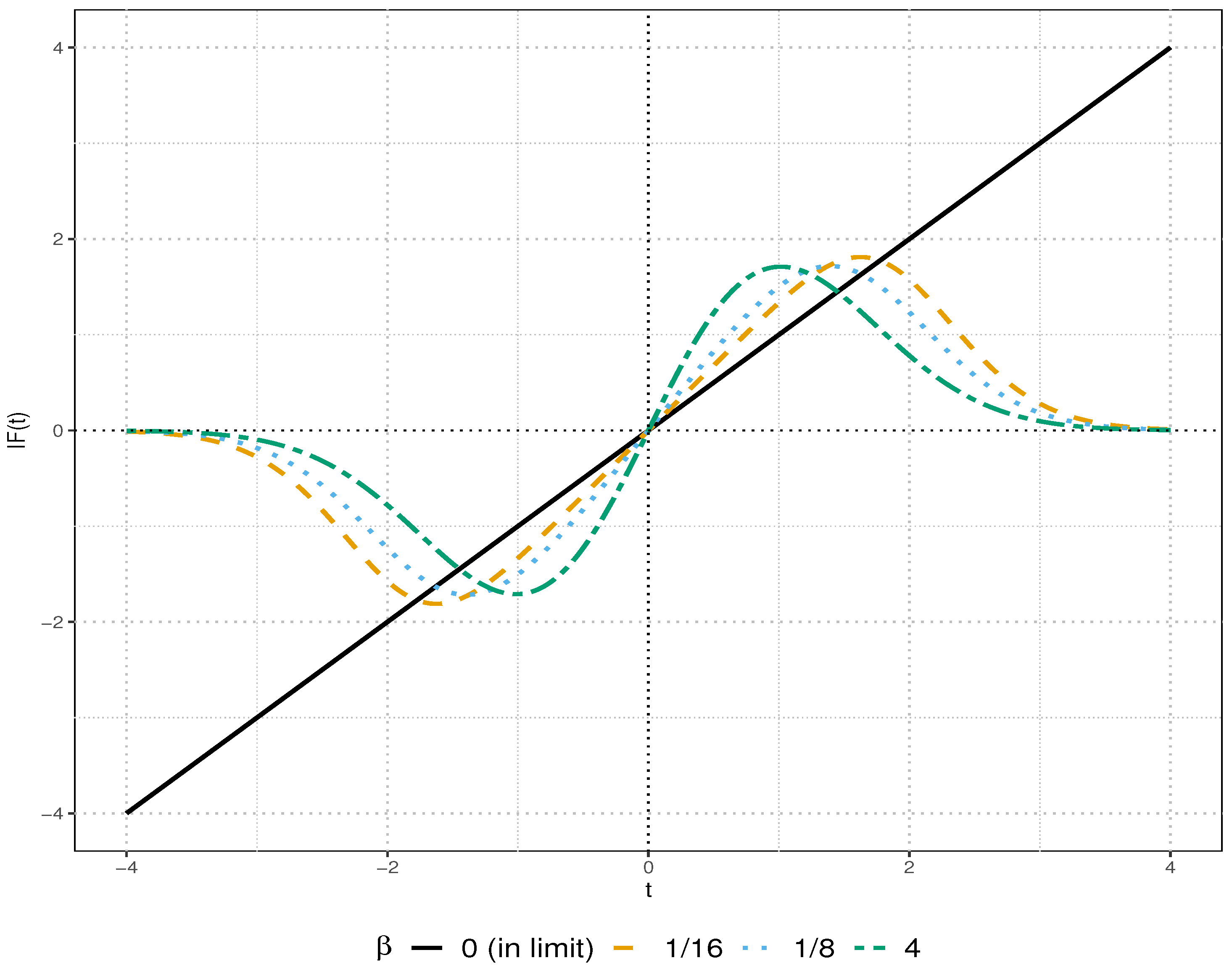
Figure 3 describes the theoretical influence function for μ ^ ( β ) —the MEWDE( β ) functional for the mean parameter of the contaminated normal distribution ( 1 ϵ ) N ( μ , 1 ) + ϵ Δ t for various contamination values t. For all β > 0 considered here, we note their bounded and redescending nature.

4. Simulation Studies for MEWDE(β)

4.1. Introduction

  For i.i.d. data, when the true density g belongs to the model, i.e., g = f θ for some θ Ω , let θ ^ refer to the MEWDE of an unknown parameter θ . For β > 0 , under the regularity conditions (1)–(7) outlined in Section 3.2, the score function satisfies the requirements of the Lindeberg–Feller Central Limit Theorem. Although this theorem [18] is typically invoked for non-identically distributed data, it remains applicable in our i.i.d. setting because the finite variance of the score function automatically satisfies the Lindeberg condition. Consequently, applying the standard Taylor expansion technique for M-estimators, we formally state that the asymptotic normality of n ( θ ^ θ ) is an s- variate normal distribution with mean vector 0 and dispersion matrix given by J 1 K J 1 , where
J = u θ ( x ) u θ T ( x ) [ 1 exp ( f θ ( x ) / β ) ] f θ ( x ) d x , K = u θ ( x ) u θ T ( x ) [ 1 exp ( f θ ( x ) / β ) ] 2 f θ ( x ) d x ξ ξ T , ξ = u θ ( x ) [ 1 exp ( f θ ( x ) / β ) ] f θ ( x ) d x .
As β 0 , both J and K reduce to the Fisher information matrix. We now consider different parametric families and compare the performance of MEWDEs and MDPDEs under different contamination scenarios.

4.2. Tuning Parameter Selection

In minimum EWD estimation, small values of β provide greater model efficiency, while large values of β provide greater outlier stability and protection against small model violations. Given any real dataset, we must choose the “optimal”, data-based tuning parameter β so that the procedure has the right amount of balance for the dataset in question. We follow the approach of [19] to derive the optimal estimate of the tuning parameter. This approach constructs an empirical estimate of the Mean Squared Error as a function of the tuning parameter β and a pilot estimator θ P given by
M S E β ^ ( θ P ) = θ ^ β θ P T θ ^ β θ P + 1 n tr Ψ n 1 θ ^ β Ω n θ ^ β Ψ n 1 θ ^ β ,
where tr ( · ) is the trace of a matrix and Ψ n and Ω n are the matrices defined in Equations (10) and (11), respectively, evaluated at θ = θ ^ β = MEWDE ( β ) . Further, tr(·) denotes the trace of a matrix. By minimizing the objective function given in Equation (17) over β > 0 , we get a data driven “optimal” estimate of the tuning parameter. Ref. [19] proposes the minimum L 2 estimator as the pilot estimator in the above calculation.

4.3. Simulation Scheme

To rigorously evaluate the finite-sample performance of the proposed MEWDE, we compared it against the minimum density power divergence estimator (MDPDE) and the classical Maximum Likelihood Estimator (MLE). We adopted an “Oracle” tuning approach for the simulation study. For each estimator and each simulation scenario (combination of sample size n and contamination level ϵ ), we performed a grid search to identify the optimal tuning parameter ( α O P T for DPD, β O P T for EWD) that minimizes the empirical Mean Squared Error (MSE). This approach reports the best possible performance achievable by each estimator, isolating the theoretical capability of the divergence measure from the variability of data-driven tuning selection. Note that the practical data-driven algorithm for selecting β in real applications is detailed in Section 4.2.

4.4. Results

We first define the empirical finite sample relative efficiency (FSRE) of the MEWDE (or MDPDE) as the ratio of MSE(MLE) to MSE(MEWDE) (or to MSE(MDPDE)). Under this metric, a value of 1.0 indicates efficiency equivalent to the MLE, while values < 1.0 indicate superior performance (error reduction) in the presence of contamination. To provide a comprehensive benchmark, we also report the performance of classical robust methods, specifically Huber’s M-estimator and Tukey’s Bisquare.
We consider three separate simulation designs involving (a) estimation of the mean of a univariate normal distribution with known standard deviation, (b) estimation of the standard deviation of a univariate normal distribution with known mean, and (c) estimation of the mean parameter of an exponential distribution. For simulation (a), the true distribution is taken to be N ( 0 , 1 ) and the contaminating distribution is N ( μ c , 1 ) . We run simulations for μ c = 3 and 5 and estimate the mean under the N ( μ , 1 ) model. Our findings are presented in Table 1. Table 1 presents the finite sample relative efficiency (FSRE) results, calculated as the ratio of the MSE of the MLE to the MSE of the robust estimator. Consequently, a value greater than 1 indicates the robust method is less efficient than the MLE, while values less than 1 (common under contamination) indicate superior performance. The results cover the pure location model with sample sizes n = 50 , 100 , 200 and contamination proportions ϵ = 0 , 0.10 , 0.20 , 0.30 .
Table 1 demonstrates that under an independent “Oracle” tuning protocol, the MEWDE offers a superior efficiency–robustness trade-off in the most common contamination regimes. In the absence of outliers ( ϵ = 0 ), the estimator retains high efficiency comparable to the MLE (FSRE 1.0 ), confirming that robustness does not come at the cost of performance under the null model. Crucially, under moderate contamination ( ϵ [ 0.1 , 0.2 ] ), the MEWDE consistently outperforms both the MDPDE and classical robust methods; for example, at n = 50 and ϵ = 0.2 , the MEWDE achieves a ten-fold reduction in MSE compared to the MDPDE (0.027 vs. 0.261), while the MDPDE exhibits greater stability in small-sample, severe-contamination settings ( n = 50 , ϵ = 0.3 ); the MEWDE recovers its superiority as sample size increases ( n = 200 ), suggesting that the exponential weight function provides sharper discrimination against outliers when sufficient data is available to stabilize the density estimate. For completeness, the full tabulated results and efficiency comparisons for Scenarios (b) and (c) are provided in Appendix C. These additional results exhibit trends consistent with Scenario (a), confirming the method’s stability across different distributional assumptions.

4.5. Sensitivity to Tuning Parameter Misspecification

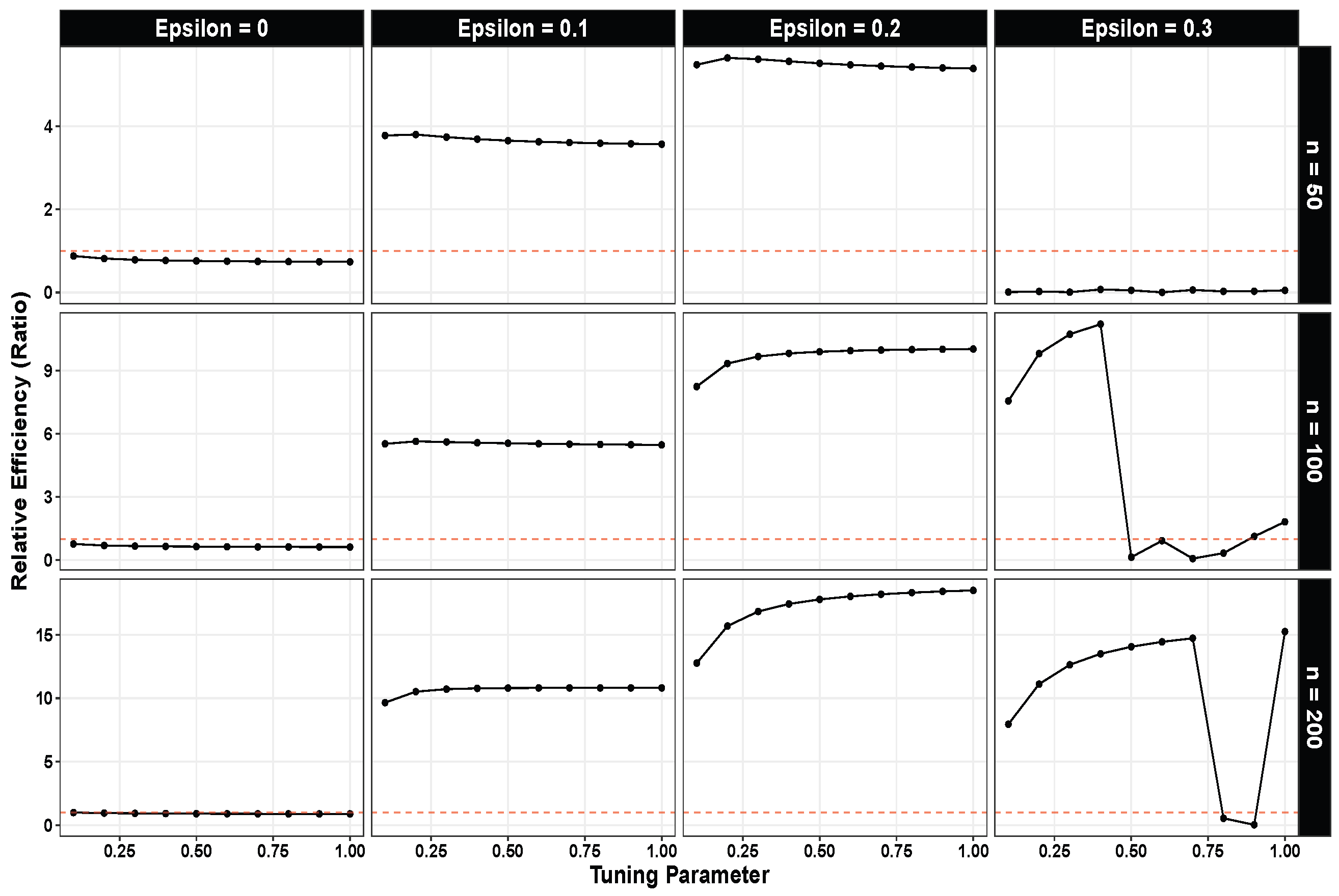
A practical concern for robust M-estimation is the sensitivity of the estimator to the choice of the tuning parameter β , while our primary results rely on an Oracle selection, practitioners require guidance on a “safe” range for β that yields robust performance without requiring prior knowledge of the contamination level. To address this, we examined the efficiency ratio defined as MSE MLE / MSE MEWDE across a grid of tuning parameters β [ 0.1 , 1.0 ] . In this metric, values greater than 1.0 indicate that the proposed estimator outperforms the non-robust MLE. We varied the sample size n { 50 , 100 , 200 } and contamination proportion ϵ { 0.0 , 0.1 , 0.2 , 0.3 } (using a mean-shift contamination N ( 3 , 1 ) ) to identify the regions of stability and breakdown. The sensitivity of the estimator is illustrated in Figure 4. In each panel, the black curve represents the MSE profile as β varies, while the vertical red dashed line marks the Oracle optimal β . The results (summarized in Figure 4) reveal three distinct performance regimes that offer concrete guidance for parameter selection:
  • Efficiency Cost (Clean Data, ϵ = 0 ): In the absence of outliers, the efficiency ratio is consistently below 1.0 , reflecting the expected cost of robustness. However, for small tuning parameters ( β [ 0.1 , 0.3 ] ), the ratio remains high (approx. 0.75 0.98 for n 50 ), confirming that the MEWDE retains the majority of the statistical information when the model is correctly specified.
  • Robustness Regime ( ϵ [ 0.1 , 0.2 ] ): Under moderate contamination, the estimator demonstrates a wide “basin of stability.” The MEWDE consistently dominates the MLE, achieving efficiency ratios between 3.0 and 17.0 across the entire range of tested β . This indicates that for the most common contamination scenarios, the method is highly insensitive to parameter misspecification; any β [ 0.1 , 1.0 ] yields superior results.
  • Severe Contamination Limit ( ϵ = 0.3 ): A critical divergence occurs under severe contamination. For small sample sizes ( n = 50 ), the estimator breaks down regardless of β , as the minority inliers are insufficient to anchor the density. However, for moderate sample sizes ( n = 100 ), we observe a clear transition: small tuning parameters ( β [ 0.1 , 0.4 ] ) maintain robustness (ratio > 7.0 ), while larger values ( β 0.5 ) lead to performance degradation.
Figure 4. Sensitivity analysis showing the Mean Squared Error (MSE) of the MEWDE as a function of the tuning parameter β for different sample sizes.
Mathematics 14 00670 g004
Based on these findings, we recommend β [ 0.1 , 0.3 ] as a default operating range. This interval minimizes efficiency loss on clean data while providing maximum protection against severe contamination in intermediate sample sizes ( n = 100 ), avoiding the breakdown risks associated with larger smoothing parameters.

4.6. Performance of Data-Driven Tuning

A common critique of minimum divergence methods is the reliance on a tuning parameter β that must be selected by the user, while the primary simulation results presented in Table 1 utilized an “Oracle” approach (selecting the β that minimizes the actual squared error) to establish the theoretical limit of the method, this is impossible in practical applications where the true parameter is unknown.
To assess the practical feasibility of the MEWDE, we implemented the data-driven tuning algorithm proposed by Warwick and Jones [19]. This method selects the optimal tuning parameter β ^ by minimizing an empirical estimate of the Asymptotic Mean Squared Error (AMSE):
β ^ = arg min β ( θ ^ β θ ^ p i l o t ) 2 + V a r ^ ( θ ^ β ) n ,
where θ ^ β is the MEWDE computed with tuning parameter β , and V a r ^ ( θ ^ β ) is the sandwich variance estimate. Crucially, this criterion requires a pilot estimator θ ^ p i l o t to approximate the bias. For this simulation, we following [19]’s proposal to use the minimum L 2 estimator as θ ^ p i l o t . The simulation setting mirrors the pure location model described in Section 4.3. We generated independent observations from a contaminated normal mixture model:
g ( x ) = ( 1 ϵ ) ϕ ( x ) + ϵ ϕ ( x 5 ) ,
where ϕ ( · ) denotes the standard normal density. We evaluated the performance across sample sizes n { 25 , 100 , 500 } and contamination proportions ϵ { 0.00 , 0.05 , 0.10 , 0.20 } . For each replicate, the data-driven algorithm selected β ^ from the grid { 0.1 , 0.2 , , 1.0 } without knowledge of the true parameter or contamination level. The results of this comparison are presented in Table 2.
The comparison between the Oracle and data-driven MEWDE is presented in Table 2. In the pure data scenario ( ϵ = 0 ), the data-driven approach incurs an efficiency loss of approximately 19–24% compared to the Oracle. However, as contamination is introduced, the performance of the data-driven tuning rapidly converges to that of the Oracle. For ϵ 0.10 , the percentage loss drops significantly, often falling below 1% (see Table 2). In these cases, the presence of outliers forces both the Oracle and the data-driven selector to adopt robust tuning parameters, eliminating the gap between the theoretical optimum and the practical estimate. This confirms that the Warwick–Jones algorithm, anchored by the minimum L 2 estimator, effectively adapts to the data structure, providing necessary robustness without requiring prior knowledge of the contamination level.

4.7. Stability in Multivariate Settings

To address concerns regarding the performance of the MEWDE as the dimensionality of the parameter space increases, we extended our simulation study to a multivariate linear regression setting. We considered models with p { 2 , 5 , 10 } predictors and contamination rates of ϵ { 0 , 0.1 , 0.2 } . As shown in Table 3, the MLE suffers from severe degradation as dimensionality and contamination increase; for example, with n = 50 , p = 10 and 20 % contamination, the MLE squared error explodes to 20.55 . In contrast, the MEWDE ( β = 0.1 ) maintains remarkable stability with an error of 0.406 , comparable to its performance on clean data. Furthermore, the results demonstrate that β = 0.1 provides an excellent trade-off, achieving near-optimal efficiency on clean data while offering full protection against vertical outliers.

4.8. Computational Complexity

The computational cost of the MEWDE is dominated by the evaluation of the objective function and its gradient at each step of the iterative solver. For a sample size n, the evaluation of the estimating equation requires summing the score function over all observations; this operation is O ( n ) . The integral term required for Fisher consistency depends only on the parameters, not the sample size, and thus adds a constant overhead O ( 1 ) per iteration (assuming fixed dimensionality). Consequently, if the numerical solver (e.g., Newton–Raphson) requires k iterations to converge, the total complexity for a fixed tuning parameter is O ( k n ) . When selecting the optimal tuning parameter β O P T via the data-driven grid search described above, the estimator is re-computed for each of the G candidate values in the grid. The total complexity for the tuning procedure is therefore O ( G k n ) . Since the grid size G and the number of iterations k are typically small and fixed relative to the sample size, the overall procedure remains linear in n, i.e., O ( n ) . This ensures that the data-driven selection of β remains computationally feasible even for large datasets, comparable to standard likelihood-based methods.
Remark 5.
The estimators were computed by solving the system of estimating equations defined in Equation (3). We utilized the multiroot  function from the  rootSolve  package in R [20], which implements a Newton–Raphson method with diagonal Jacobian approximation. The convergence tolerance was set to 10 8 . This root-finding approach proved to be numerically stable and computationally efficient, with average runtimes comparable to standard M-estimation routines and no significant overhead compared to the MDPDE.
Remark 6.
Under light or no contamination, the MEWDE and MDPDE exhibit nearly indistinguishable performance, as expected given their shared first-order efficiency at the model. The practical advantage of the EWD becomes apparent primarily in moderate to heavy contamination settings, where bounded weighting prevents both outlier influence and inlier over-emphasis.

5. Modeling Real Data

To ensure a comprehensive evaluation, we compare our proposed MEWDE against the standard MDPDE as well as classical robust estimators, specifically Huber and Tukey’s Bisquare estimators. We also report the ML + D (Outlier-Deleted Maximum Likelihood Estimator), which serves as a “clean” benchmark calculated after manually removing the identified outliers from the dataset.

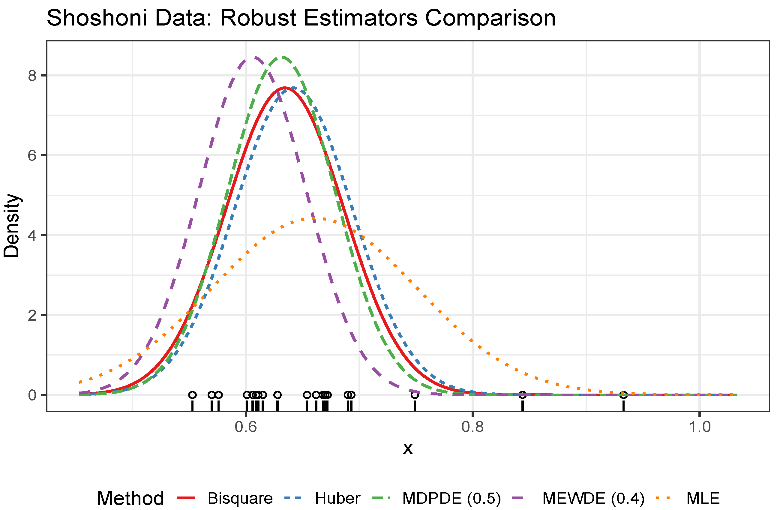
5.1. Shoshoni Rectangles

We consider the data on Shoshoni rectangles presented and analyzed by [21]. The parameter estimates for the Shoshoni dataset are summarized in Table 4 and visualized in Figure 5. The results clearly illustrate the sensitivity of the classical Maximum Likelihood Estimator (MLE) to extreme values compared to the robust alternatives. The MLE yields the largest location and scale estimates ( μ ^ MLE 0.661 , σ ^ MLE 0.090 ), indicating that the fit is being pulled toward the right-skewed outliers inherent in the data. This inflation of the standard deviation results in a density curve that is overly dispersed and fails to capture the mode of the bulk data. In contrast, the M-estimators (Huber and Bisquare) and the divergence-based estimators (MDPDE and MEWDE) provide significantly tighter fits. Both the Huber and Bisquare methods reduce the location estimate to approximately 0.63 0.64 and nearly halve the estimated scale to σ ^ 0.052 . The divergence-based estimators demonstrate the strongest robustness profiles. The MDPDE ( α = 0.5 ) and MEWDE ( β = 0.4 ) produce the smallest scale estimates ( σ ^ 0.047 ), suggesting they have successfully trimmed the influence of the outliers to focus on the central density. Notably, the MEWDE provides the most distinct location estimate ( μ ^ MEWDE 0.606 ), shifting the center further to the left than the other methods. This suggests that the MEWDE with β = 0.4 is highly effective at identifying the core underlying distribution, virtually ignoring the influence of the larger values that skew the standard MLE.

5.2. Drosophila Offspring Counts

We compare the performance of the MEWDE and MDPDE in the context of data on fruit flies (see [22]). In this experiment male flies were sprayed with a chemical, and then made to mate with unexposed females. The response, for each father fly, was the number of daughter flies having a recessive lethal mutation in the X-chromosome.
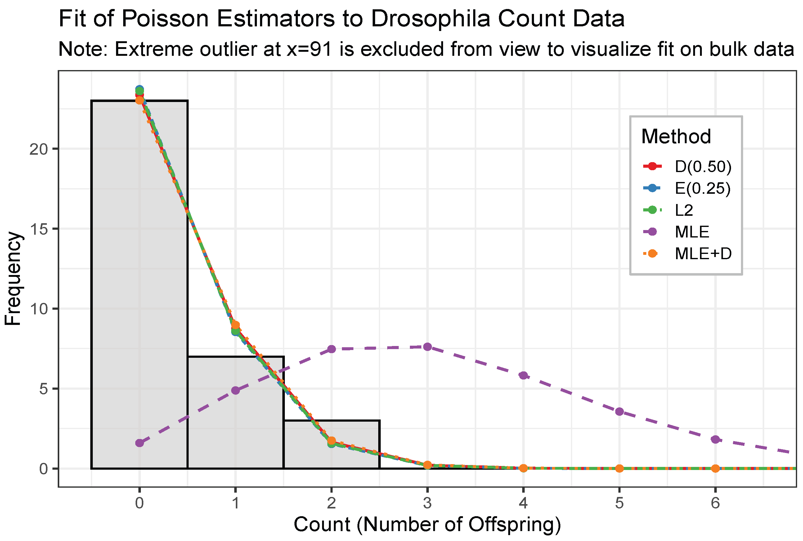
The frequencies of these responses (presented in the first row of Table 5) are modeled as Poisson variables, and the estimates of the Poisson mean parameter λ (as well as the estimated frequencies), using several members of the DPD and EWD families, the MLE and the MLE + D (outlier-deleted MLE) are presented in Table 5. The single extreme value at 91 is treated as the obvious outlier. Both sets of estimators have comparable (satisfactory) performance, which adequately discount the outlier. To visually assess the impact of the extreme outlier on model adequacy, Figure 6 overlays the fitted Poisson densities on the observed count frequencies, illustrating the divergence-based estimators’ superior fit to the bulk data compared to the MLE.

5.3. Homicide from Firearm Use and GDP

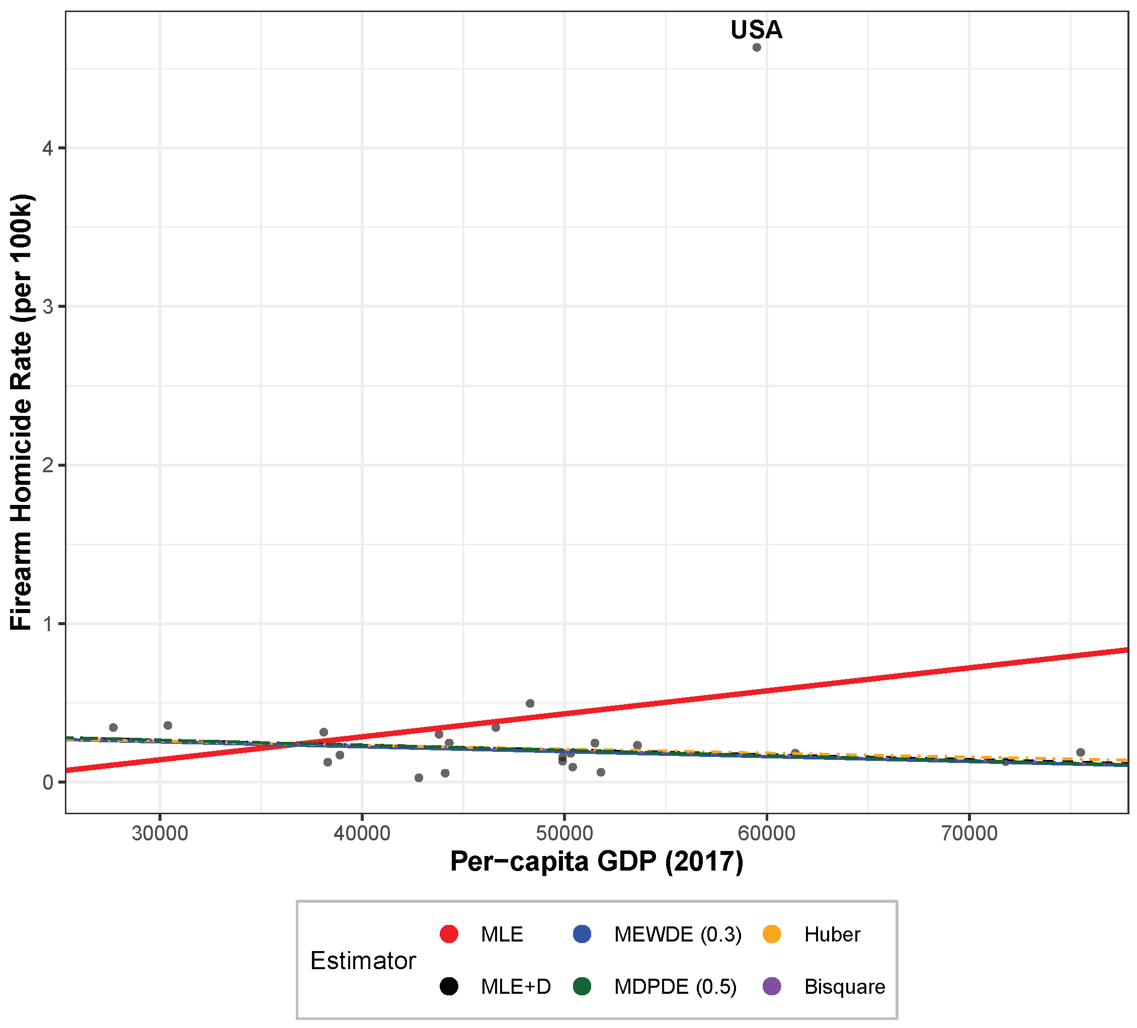
We consider modeling age-standardized national firearm-related homicide rates in 23 Western countries as a function of per-capita gross domestic product as of 2017. Country-specific information on firearm-related homicide rates (from [23]) and GDP (from [24]) were obtained. Figure 7 displays the scatter plot of firearm-related homicide rates against per-capita GDP, revealing the United States as a significant outlier that severely distorts the standard MLE, resulting in a counter-intuitive positive slope estimate of 1.45 × 10 5 . In contrast, as summarized in Table 6, all robust estimators—including Huber, Bisquare, MDPDE, and the proposed MEWDE—successfully identify and downweight this leverage point, recovering the negative relationship observed in the outlier-deleted benchmark (ML + D). Notably, MEWDE achieves the lowest scale estimate ( σ 0.102 ) among all robust competitors, indicating it provides the tightest fit to the majority of the data.

5.4. Solubility of Alcohols in Water

We consider fitting a multiple linear regression model to the dataset concerning alcohol solubility in water (see [25]). The dataset gives, for 44 aliphatic alcohols, the logarithm of their solubility together with three physicochemical characteristics (namely, solvent accessible surface-bounded molecular volume (SAG), mass and volume). The interest is in predicting the solubility. Following the authors’ suggestion of fitting an MM regression-based model to the data, we observe that four data points (roughly 10 % of the dataset) are assigned much smaller ‘robustness weights’ as compared to the remaining 40 data points. Treating these four observations as outliers, we obtain the Huber and Bisquare estimates of the regression coefficients and error standard deviation. We also compute the robust LMS estimate. In order to estimate the error s.d. σ , we compute σ ^ = median | r i median ( r i ) | / 0.67449 . Finally, we compute minimum EWD( β ) regression parameter estimates for various values of β . Our findings are presented in Table 7.
As a visual inspection is not possible for the fits in this multiple linear regression model, the coefficients of Table 7 are not sufficient on their own to give a full idea about how stable and outlier-resistant the fits are. By means of Figure A5 and Figure A6 in the Appendix B, we examine the residuals of each of the fits for the data and explore how well they fare in terms of separating out the outliers. Figure A5 and Figure A6 demonstrate a particular MEWDE and the LMS estimate are much more successful in making the outliers stand out and giving stable fits compared to the least squares fit provided by the MLE.

5.5. Tuning Parameters for the Data Examples Considered

Through the procedure outlined in Section 4.2, the optimal tuning parameter for the data on Shoshoni rectangles is found to be β OPT = 0.43 , and the associated estimated parameters are μ ^ = 0.63 and σ ^ = 0.05 . The corresponding (sample size-scaled) asymptotic Mean Squared Error is 5.07 × 10 3 . For the data on Drosophila fruit flies, the optimal tuning parameter is found to be β O P T = 0.08 , and the estimated mean parameter is λ ^ = 0.377 . The corresponding (sample size-scaled) asymptotic Mean Squared Error is 0.46 . For the data on firearm-related homicide and GDP, the optimal tuning parameter is β O P T = 1.6 , and the corresponding estimated regression parameters (intercept, GDP, error standard deviation) are ( 0.416 , 3.932 × 10 6 , 0.066 ) . Finally, for the data on alcohol solubility, the optimal tuning parameter is β O P T = 0.66 , and the corresponding estimated regression parameters intercept, SAG, volume, mass, error standard deviation are ( 6.084 , 0.112 , 0.135 , 0.174 , 0.062 ) , respectively.

6. Testing of Hypotheses

6.1. Introduction

Here we develop general robust tests of the hypotheses based on Bregman divergences. This generalizes the works of [15,16]. We establish the asymptotic null distribution of the proposed test statistic and apply the theory developed to a real-life dataset. Our focus will remain on EWD( β ).
Unlike the previous sections, we will consider the case of i.i.d. data only. We begin with an identifiable parametric family of probability measures P θ on a measurable space { χ , A } with an open parameter space Ω R s , s 1 . Measures P θ are described by densities f θ = d P θ / d μ , absolutely continuous with respect to a dominating σ -finite measure μ on χ . We have an i.i.d. sample of size n given by X 1 , X 2 , , X n from a density belonging to the family F θ = { f θ : θ Ω } . We will assume that the support of the distribution is independent of θ . The hypothesis of interest is H 0 : θ Ω 0 against H 1 : θ Ω 0 . We use the common approach where the restricted parameter space specified by H 0 can be rewritten by a set of r < s restrictions of the form
m ( θ ) = 0 r
on Ω , where m : R s R r is a vector valued function such that the s × r matrix M ( θ ) = m T ( θ ) θ exists and is continuous in θ and rank( M ( θ ) ) = r .

6.2. The Test Statistic

To perform this test of the hypotheses, we first obtain θ ^ B 1 , the unrestricted minimum Bregman divergence estimator for a given B 1 function and then obtain the restricted estimator θ ˜ B 1 , subject to the constraints of Equation (19). We then examine the family of Bregman divergence test statistics (BDTS)
T B 2 ( θ ^ B 1 , θ ˜ B 1 ) = 2 n × D B 2 ( f θ ^ B 1 , f θ ˜ B 1 ) ,
where D B 2 ( g , f ) is the Bregman divergence between two densities g and f, defined in Equation (1) with B 2 as the B function. We will consider the functions B 1 and B 2 to have the same functional form (e.g., as given by the exponentially weighted divergences) only differing, if at all, in the values of their tuning parameters. Thus, in the derivation of the asymptotic distribution of the test statistics, the functions B 1 and B 2 are allowed to be different. In practice, however, a single, suitably chosen common function B will generally work well in most cases.
In addition to Assumptions 1–5 presented in Section 3.2, we make the following assumption.
Assumption 8.
For all θ ω , the partial derivatives 2 m l ( θ ) / θ j θ k are bounded for all j, k and l, where m l ( · ) is the l-th element of m ( · ) .
Theorem 2.
Under Assumptions 1–5 and 8, and assuming that the true distribution belongs to the model, i.e., G = F θ g for some θ g Ω which satisfies the set of constraints given by Equation (19), the constrained minimum Bregman divergence estimator θ ˜ n , B 1 has the following properties: the underlying B function is denoted by B 1 .
1. 
Consistency: θ ˜ n , B 1 P θ g as n .
2. 
Asymptotic normality: The asymptotic null distribution of n ( θ ˜ n , B 1 θ g ) is s-dimensional multivariate normal with the zero mean vector and an s × s dispersion matrix Σ B 1 = P B 1 K B 1 P B 1 , where K B 1 is the i.i.d. analogue of the Ω n matrix defined by Equation (11) with B 1 serving as the B function. The P B 1 matrix is defined as P B 1 = J B 1 1 Q B 1 M J B 1 1 , where J B 1 is the i.i.d. analogue of the Ψ n matrix defined by Equation (10). Further, Q = J B 1 1 M [ M T J B 1 1 M ] 1 ; M = M ( θ ) is as defined in Section 6.1.
The proof is provided in Appendix D.
Remark 7.
Theorem 2 extends Theorem 1 in the context of i.i.d. data. Under the setup of Theorem 1, M becomes a null matrix and consequently, P B 1 = J B 1 1 and the asymptotic dispersion matrix of the unrestricted minimum Bregman divergence estimator assumes the form specified by Theorem 1.
Theorem 3 presents the asymptotic distribution of the test statistic defined in Equation (20).
Theorem 3.
Under Assumptions 1–5 and 8, the asymptotic distribution of the test statistic defined in Equation (20) is identical with, under the null hypothesis specified in Equation (19), the distribution of the random variable
i = 1 k λ i ( B 1 , B 2 , θ ) Z i 2 ,
where Z 1 , , Z k are independent standard normal variables and λ i ( B 1 , B 2 , θ ) for i = 1 , , k are the nonzero eigenvalues of the matrix A B 2 B B 1 K B 1 B B 1 , and k is the rank of the matrix B B 1 K B 1 B B 1 A B 2 B B 1 K B 1 B B 1 . The ( i , j ) -th element of A B 2 is defined as follows:
A B 2 ( i , j ) = B 2 ( f θ g ( x ) ) f θ g ( x ) θ i f θ g ( x ) θ j d x
and the matrix B B 1 is equal to
J B 1 1 M [ M T J B 1 1 M ] 1 M T J B 1 1 .
The proof is provided in Appendix D.
Remark 8.
We note that the ranks of B B 1 K B 1 B B 1 A B 2 B B 1 K B 1 B B 1 , B B 1 K B 1 B B 1 and M are simultaneously equal to r.
Remark 9.
An easy way to approximate the required critical region of the above test is outlined here. From Theorem 3 it is obvious that the k eigenvalues described are functions of θ g . Under the null, they can be consistently estimated by plugging in θ ˜ B 1 in place of θ g . Let these estimated eigenvalues be λ ^ 1 , , λ ^ k . Generating k independent observations Z 1 , , Z k from the N ( 0 , 1 ) distribution, one can approximate the quantiles of i λ ^ i Z i 2 by replicating this procedure a large number of times, which can then serve as consistent estimates of the quantiles of the limiting variable in Equation (21).
Remark 10.
An approximate form of the power function of the test statistic can be obtained by following the steps outlined by Theorem 7 of [16].
Remark 11.
While Theorem 3 derives the asymptotic null distribution of the Bregman Divergence Test Statistic (BDTS), the resulting distribution involves a weighted sum of independent chi-square variables, where the weights depend on the unknown true density. In finite samples, estimating these weights can be computationally demanding and may lead to size distortions. To provide a readily implementable and precisely calibrated inference tool, we employ a parametric bootstrap approach. For testing the hypothesis H 0 : μ = 0 against H 1 : μ > 0 , the procedure is as follows:
1. 
Compute the robust estimate μ ^ o b s from the observed data using the MEWDE. The test statistic is defined as T o b s = μ ^ o b s .
2. 
Generate B bootstrap samples X 1 * , , X B * from the null distribution N ( 0 , 1 ) .
3. 
For each bootstrap sample, compute the estimate μ ^ b * and the statistic T b * = μ ^ b * .
4. 
Compute the p-value as 1 B b = 1 B I ( T b * T o b s ) .
This procedure ensures that the test maintains the nominal size α under the null hypothesis while inheriting the robustness properties of the estimator.

6.3. Comparative Power Analysis: Simulation Design and Findings

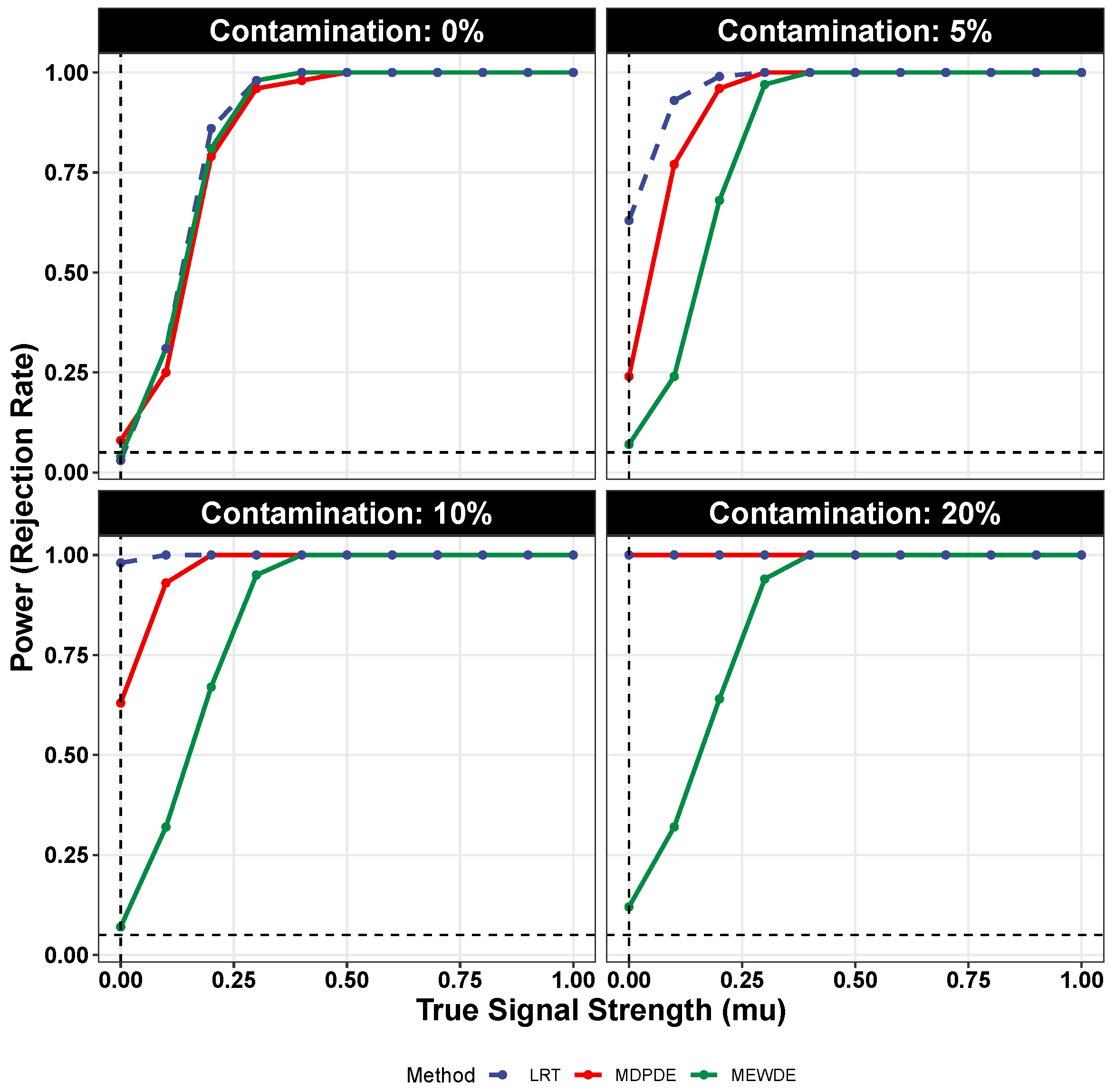
To explicitly evaluate the performance of the MEWDE against the established density power divergence (MDPDE) and the classical likelihood ratio test (LRT), we conducted a matched-efficiency power simulation. The data were generated from a contaminated normal model ( 1 ϵ ) N ( μ , 1 ) + ϵ N ( 3 , 1 ) , where μ represents the signal strength varying from 0.0 to 1.0 . We fixed the sample size at n = 100 and considered contamination levels ϵ { 0 , 0.05 , 0.10 , 0.20 } . A critical aspect of this comparison is ensuring that the robust estimators are tuned fairly. We selected a standard robust tuning parameter for the MDPDE ( α = 0.30 ) and determined the corresponding MEWDE parameter ( β = 0.10 ) that yields an identical Mean Squared Error (MSE) under the clean null model ( N ( 0 , 1 ) ). This calibration ensures that any observed differences in power or stability are attributable to the properties of the divergence measures rather than unequal efficiency trade-offs. Figure 8 displays the empirical power curves for the three methods. The results highlight two key findings:
  • Efficiency Matching for Clean Data: In the absence of contamination (0% panel), the power curves for the MEWDE and MDPDE are virtually indistinguishable and lie slightly below the optimal LRT. This confirms the success of our calibration strategy and demonstrates that the MEWDE incurs no additional efficiency cost compared to the DPD when the model is correctly specified.
  • Superior Robustness of Validity: In the contaminated scenarios, the differentiation between methods becomes clear. The classical LRT exhibits catastrophic size distortion, rejecting the null nearly 100% of the time at μ = 0 . The MDPDE, while significantly more robust than the LRT, still suffers from observable size inflation (higher Type I error) in the presence of outliers. The MEWDE uniquely maintains much better control of the nominal size (≈0.05) at the null across all contamination levels. This confirms that the MEWDE offers superior robustness of validity, successfully decoupling inference from contamination where even the standard robust competitor (DPD) shows sensitivity.

6.4. An Example: Testing of Hypothesis for the Shoshoni Data

The Shoshoni data, considered earlier in Section 5.1, are assumed to come from a N ( μ , σ 2 ) distribution with both location and scale parameters being unknown. Following the benchmark analysis of this dataset by Hettmansperger and McKean [21], we consider the null hypothesis H 0 : μ = 0.618 versus H 0 : μ 0.618 . We adopt this specific null value to ensure our robust testing results are directly comparable to the findings reported in the original analysis. Ref. [21] notes that if we were to implement the outlier-sensitive likelihood ratio test for the hypothesis
H 0 : μ = 0.618 versus H 1 : μ 0.618 ,
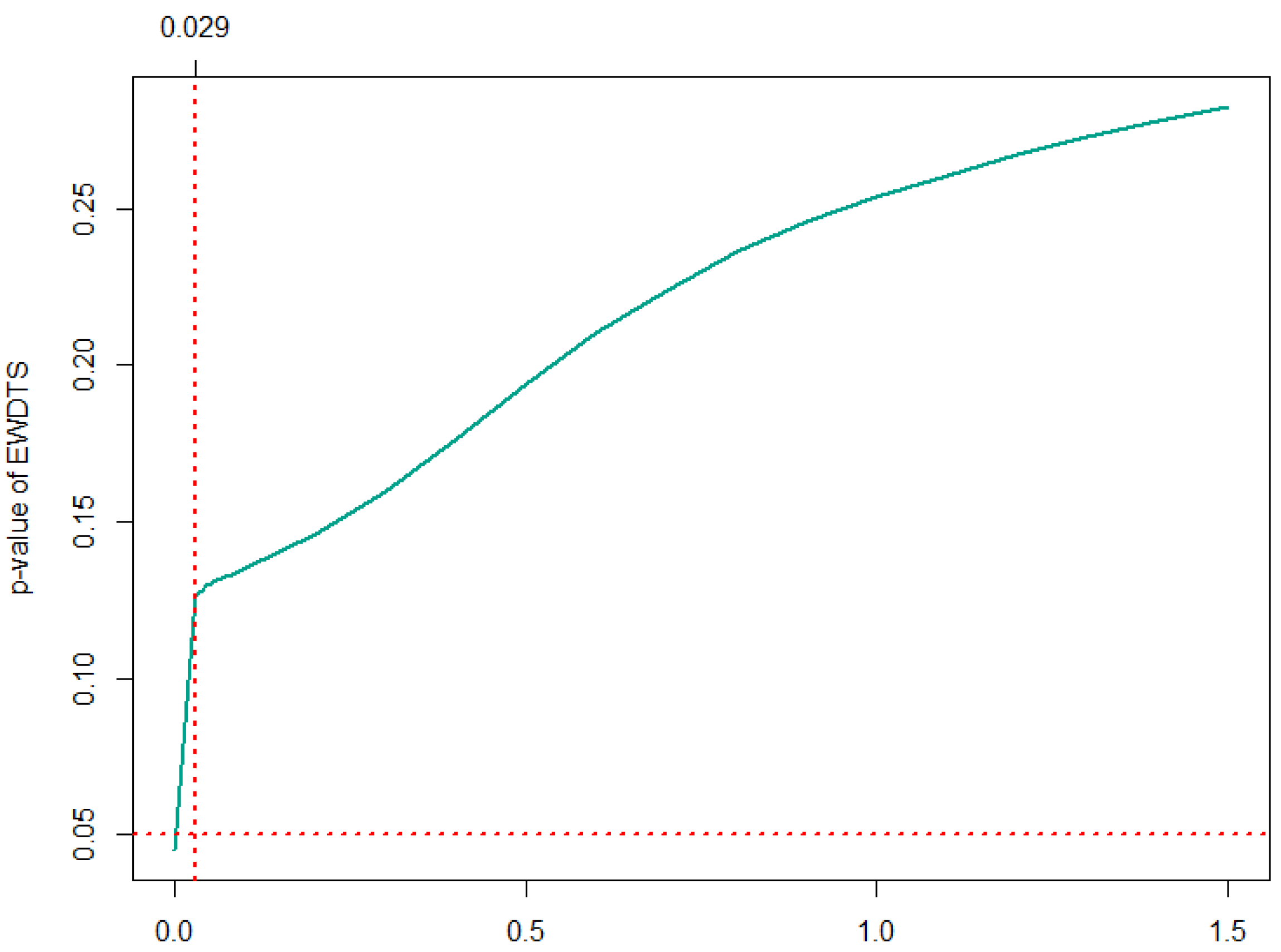
we would get a p-value of 0.053, which is at the borderline of significance at 5% level. On the other hand, the non-parametric one-sample sign test returns an entirely insignificant p value of 0.823. It would be interesting to investigate the performance of the robust test statistic presented in Section 6.2 in this context. In particular, we focus on the test statistic obtained by setting B 1 = B 2 = B , where B is the function corresponding to the exponentially weighted divergence, as defined in Equation (5). We term the test statistic so obtained as the exponentially weighted divergence test statistic (denoted by EWDTS( β )) and compute it for varying values of β > 0 . For β 0 , the test resembles the standard likelihood ratio test and returns a p-value slightly exceeding the 0.05 threshold, as reported by [21]. As β increases, the p-value quickly becomes highly insignificant, indicating that the borderline significance under the likelihood based methods is driven by the outliers. Note that the p-value for the t-test statistic for the data with three outliers removed is 0.329 , which conforms to the p-values of the EWDTS for moderately large values of β . The graph of the p-values (Figure 9) demonstrates the outlier stability of EWDTS for large values of β .

7. Closing Remarks

In this paper, we have presented an estimator based on a sub-class of density-based Bregman divergences, which is seen to be outperforming the existing standard (i.e., the DPD-based estimator). We have shown several asymptotic and distributional properties of the proposed estimator, both in the context of i.i.d data as well as independent and non-homogeneous data. A special case of linear regression (both simple and multiple) has been explored in the context of real data. We have also discussed “judicial” choice(s) of the tuning parameter which, when chosen properly, yields highly robust and efficient estimators which can often dominate the MDPDE. We have also considered an hypothesis testing strategy for parametric models which may serve as robust alternatives to the classical likelihood ratio and other likelihood-based tests. As we have noted, when the weight function generated by EWD converges to 1 as its argument, the value of the density function increases. We feel that this is the more balanced way for weighting the observations, rather than the weighing provided by the DPD, where the weights increase indefinitely with increase in the value of the density.

7.1. Practical Recommendations for Practitioners

Based on the theoretical properties and empirical results presented in this work, we offer the following guidelines for practitioners choosing between the proposed MEWDE and existing alternatives like the MDPDE:
  • Hypothesis Testing and Size Control: The MEWDE is strictly preferable in hypothesis testing scenarios where controlling the Type I error rate is critical (e.g., regulatory clinical trials). As demonstrated in the power analysis (Figure 8), the MEWDE maintains the correct nominal size (≈0.05) even under heavy contamination, whereas the MDPDE can suffer from size inflation.
  • Interpretation of Weights: In settings involving high-leverage points, the MEWDE offers a safer interpretation of “downweighting.” The exponentially decaying weight function w ( t ) = 1 exp ( t / β ) is strictly bounded in [ 0 , 1 ] , ensuring that no observation—regardless of how well it fits the model—can exert undue influence. This contrasts with power-divergence weights, which can theoretically grow unbounded depending on the model parameterization.
  • Implementation in Complex Models: For practitioners concerned with the integration burden of the asymptotic null distribution, we recommend the parametric bootstrap approach detailed in Section 6.2. This method is computationally stable, integrates easily with existing statistical software (requiring only a standard optimization routine), and avoids the complexity of estimating the eigenvalues of the weighted chi-square distribution.

7.2. Diagnostics for Model Failure

Since the theoretical guarantees of the MEWDE rely on the compatibility between the assumed model family and the bulk of the data, practitioners should monitor the resulting robust weights ( w i ) as a post hoc diagnostic. In a successful fit, weights should cluster near 1 for inliers and near 0 for outliers. A specific failure mode occurs in “heavy-tailed” settings (e.g., Cauchy data modeled as normal) where the tails of the data far exceed the support of the model. In this case, the estimator may attempt to flatten the density to accommodate the spread, causing the estimated density values f θ ( x i ) to become negligible for all points. This results in a weight collapse, where the contributing weights w i 0 . Practitioners observing consistently low weights across the sample should interpret this as a signal that the chosen parametric family is insufficiently heavy-tailed for the data, necessitating either a different model family (e.g., t-distribution) or a breakdown-point estimator such as LTS.

7.3. Limitations

While the MEWDE demonstrates strong robustness against outliers and contamination within the support of the distribution, it is important to acknowledge certain theoretical limitations. First, like most M-estimators derived from the exponential family, the validity of the asymptotic theory (specifically Assumptions 5–7 relies on the integrability of the weighted score function). In settings with extremely heavy-tailed data (e.g., Cauchy-distributed errors) or severe leverage points where the underlying moments do not exist, the required integrals may diverge. In such pathological cases, high-breakdown methods such as Least Trimmed Squares (LTS) or MM-estimators may be more appropriate, albeit at the cost of efficiency. Second, the current formulation of the EWD focuses on the standard p < n regime; as noted earlier, extending this framework to high-dimensional settings ( p n ) requires the incorporation of sparsity-inducing penalties, which is a subject of our ongoing research.

7.4. Future Work

It may also be mentioned that the proposal based on the EWD has the potential to be useful in all the situations where the DPD has been successfully applied, such as generalized linear models, survival analysis and Bayesian inference, to name a few. We hope to pursue all of these in our future research. A systematic comparison of alternative bounded weight functions within the Bregman framework is another interesting direction for future research, but lies beyond the scope of the present paper. In case of hypothesis testing, we have only investigated the analogues of the likelihood ratio tests. Other Wald-type tests based on the EWD should also be studied which are likely to have simpler asymptotic null distributions compared to that in Equation (21). The DPD-based Wald-type test has been extensively used in the literature, and comparisons with EWD-based tests will be interesting. We also hope to refine the tuning parameter selection strategy using the recently developed method of [26].
Author Contributions

Conceptualization, S.P. and A.B.; methodology, S.P. and A.B.; software, S.P.; validation, S.P. and A.B.; formal analysis, S.P. and A.B.; writing—original draft preparation, S.P.; writing—review and editing, A.B.; visualization, S.P.; supervision, A.B. All authors have read and agreed to the published version of the manuscript.

Funding

This research received no external funding.

Data Availability Statement

The data presented in this study are openly available in a Github repository: https://github.com/soumikp/2025_mathematics (accessed on 2 February 2026).

Acknowledgments

This research was supported in part by the University of Pittsburgh Center for Research Computing and Data, RRID:SCR022735, through the resources provided. Specifically, this work used the HTC cluster, which is supported by NIH award number S10OD028483.

Conflicts of Interest

The authors declare no conflicts of interest.

Abbreviations

The following abbreviations are used in this manuscript:
BDTSBregman Divergence Test Statistic
DPDDensity Power Divergence
EWDExponentially Weighted Divergence
EWDTSExponentially Weighted Divergence Test Statistic
FSREFinite Sample Relative Efficiency
GDPGross Domestic Product
IIDIndependent and Identically Distributed
LMSLeast Median of Squares
MDPDEMinimum Density Power Divergence Estimator
MEWDEMinimum Exponentially Weighted Divergence Estimator
MLEMaximum Likelihood Estimator
MSEMean Squared Error
PDFProbability Density Function
SAGSolvent Accessible Surface-bounded Molecular Volume

Appendix A. The B Function of EWD(β)

B ( x ) = x 2 β n = 0 ( x / β ) n ( n + 2 ) ! ( n + 1 ) = x 2 β n = 2 ( x / β ) n 2 ( n ) ! ( n 1 ) = x 2 β β 2 x 2 n = 2 ( x / β ) n ( n ) ! 0 1 t n 2 d t = β 0 1 1 t 2 n = 2 ( x t / β ) n ( n ) ! d t = β 0 1 exp ( x t / β ) 1 + x t β t 2 d t = β 0 1 exp ( x t / β ) 1 + x t β t 2 d t = x 0 x / β exp ( t ) 1 + t t 2 d t = x exp ( t ) 1 + t t 0 x / β 0 x / β exp ( t ) 1 t d t ] = x [ I 1 I 2 ]
where
x · I 1 = β β exp ( x / β ) x ,
and
x · I 2 = x 0 x / β exp ( t ) 1 t d t = x lim Δ 0 Δ exp ( t ) 1 t d t x / β Δ exp ( t ) 1 t d t = x { lim Δ [ log ( Δ ) [ exp ( Δ ) 1 ] + 0 Δ log ( t ) exp ( t ) d t x / β Δ exp ( t ) t d t + log Δ x / β ] } = x lim Δ log ( Δ ) exp ( Δ ) + 0 log ( t ) exp ( t ) d t x / β exp ( t ) t d t log ( x / β ) = x · [ 0 γ Γ ( 0 , x / β ) log ( x / β ) ] = x · [ γ + Γ ( 0 , x / β ) + log ( x / β ) ] .
Here γ is the Euler–Mascheroni constant, usually defined as
γ = lim n k = 1 n 1 k log n = 0 exp ( x ) log ( x ) d x ,
and Γ ( α , β ) is the incomplete Gamma integral defined as
Γ ( α , β ) = β y α 1 exp ( y ) d y .
Finally, we can write
B ( x ) = x 2 β n = 0 ( x / β ) n ( n + 2 ) ! ( n + 1 ) = x [ I 1 I 2 ] = x + γ x + β β exp ( x / β ) + x Γ ( 0 , x / β ) + x log ( x / β ) .

Appendix B. Additional Examples of Simple Linear Regression

Appendix B.1. Hertzsprung–Russell Star Cluster Data

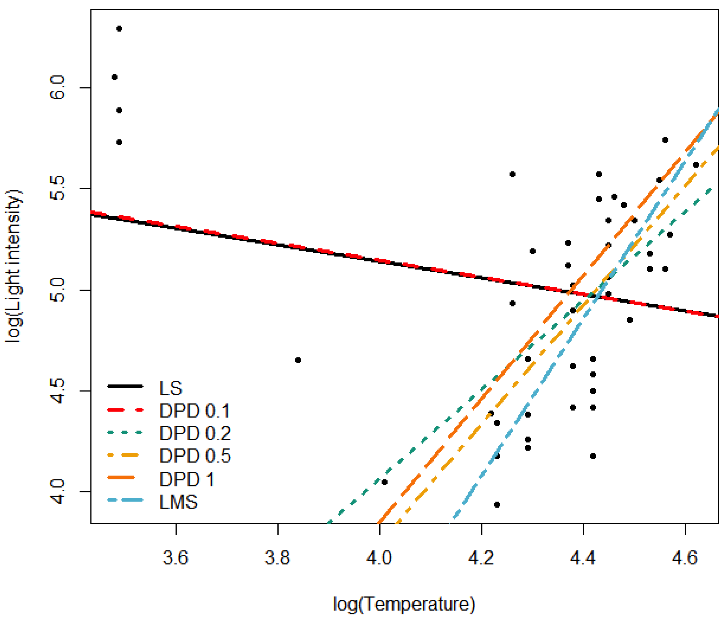
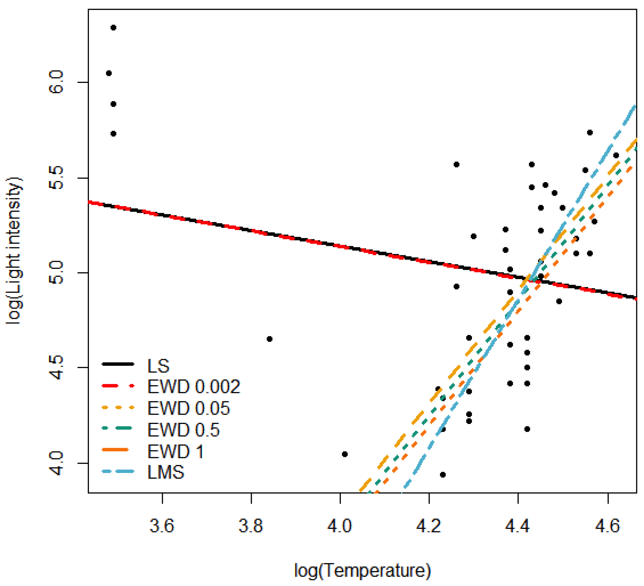
We consider the data for the Hertzsprung–Russell diagram of the star cluster CYG OB1 containing 47 stars in the direction of Cygnus (Table 3, Chap. 2 [27]). For these data the independent variable x is the logarithm of the effective temperature at the surface of the star ( T e ), and the dependent variable y is the logarithm of its light intensity ( L / L 0 ). The data were thoroughly studied by [27] who inferred that there are two groups of data points — four data points (in the top right corner of the scatter plot) clearly form a separate group in comparison with the rest of the data points. These data points are known as giants in astronomy. So, these outliers are not recording errors but are actually leverage points with the interpretation that the data are coming from two different groups. Estimates of the linear regression parameters obtained by the minimum DPD and minimum EWD methods are presented in Table A1 and Table A2, respectively.
Table A1. θ ^ for Hertzsprung–Russell dataset using MDPDE(D( α )).
EstimatesMLED(0.01)D(0.05)D(0.1)D(0.25)D(0.5)D(1)
Intercept 6.793 6.796 6.803 6.816 5.797 8.027 8.405
Slope 0.413 0.414 0.415 0.417 2.440 2.943 3.062
Error s.d. 0.565 0.554 0.560 0.566 0.405 0.393 0.392
Table A2. θ ^ for Hertzsprung–Russell dataset using MEWDE(E( β )).
EstimatesMLEE(0.01)E(0.05)E(0.1)E(0.25)E(0.5)E(1)
Intercept 6.793 6.795 8.236 8.395 8.537 8.408 8.373
Slope 0.413 0.414 2.988 3.024 3.057 3.014 2.993
Error s.d. 0.565 0.561 0.355 0.359 0.376 0.213 0.123
Based on Figure A1 and Figure A2, we observe that:
  • Clearly the estimators corresponding to α = 0 and β = 0 (which are identical and also coincide with the ordinary least squares estimators) are pulled away significantly by the four leverage points and hence it is not possible to separate out the two groups of data by looking at the corresponding residuals.
  • The MDPDE with α 0.25 can successfully ignore the outliers to give excellent robust fits that are much closer to the fit generated by the LMS estimates.
  • The MEWDE with β 0.05 are strongly robust with respect to the outliers, giving excellent fits to the remaining observations.
  • For both MDPDE and MEWDE methods, based on the residuals, we can also separate out the two groups of observations—four large residuals correspond to the four giant stars.
Thus the analysis based on DPD and EWD give stable and competitive inference in this case.
Figure A1. Data points and fitted regression lines for Hertzsprung–Russell star cluster data using least squares and minimum DPD estimates.
Mathematics 14 00670 g0a1
Figure A2. Data points and fitted regression lines for Hertzsprung–Russell star cluster data using least squares and minimum EWD estimates.
Mathematics 14 00670 g0a2

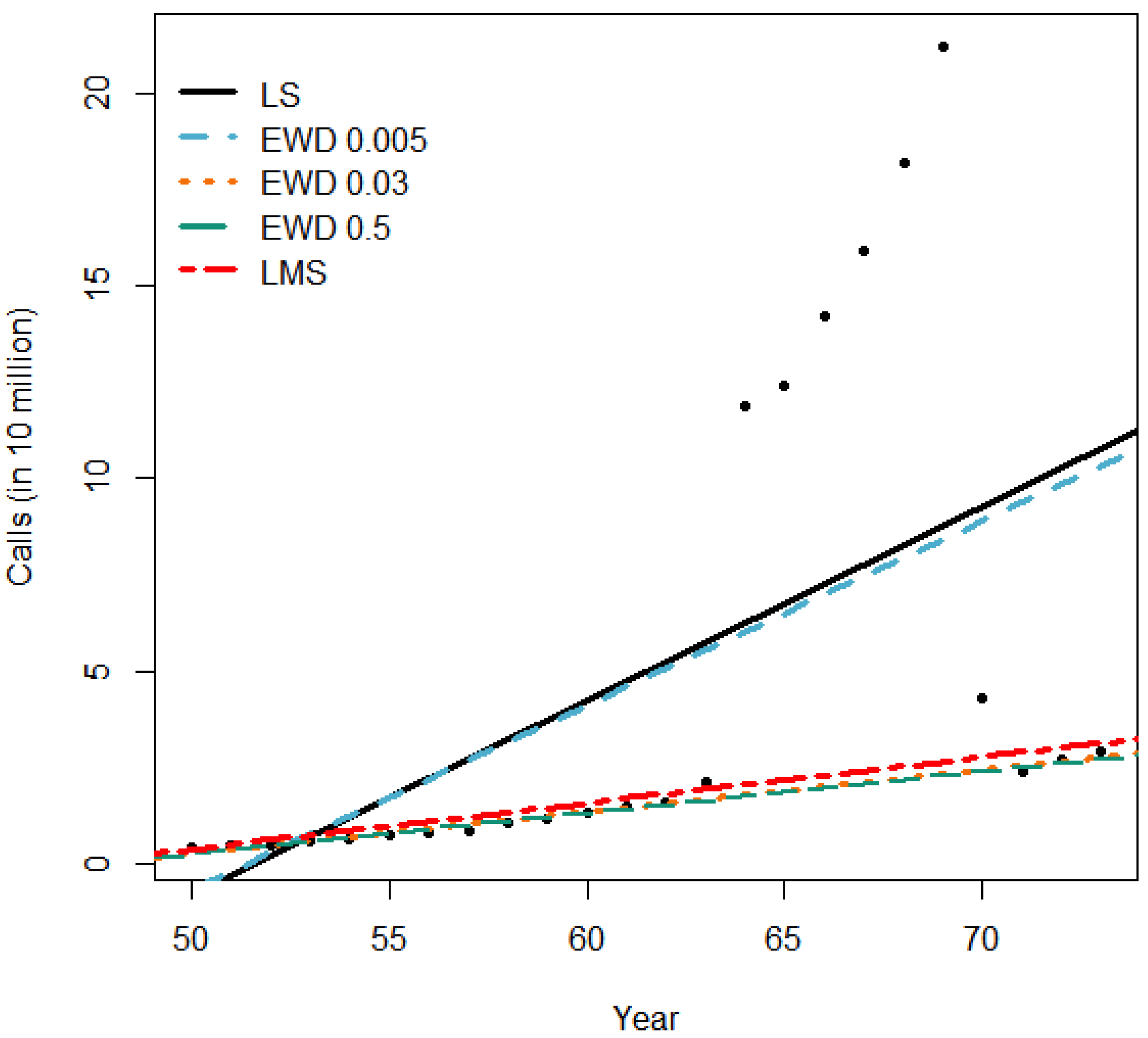
Appendix B.2. Number of International Telephone Calls in Belgium (1950–1973)

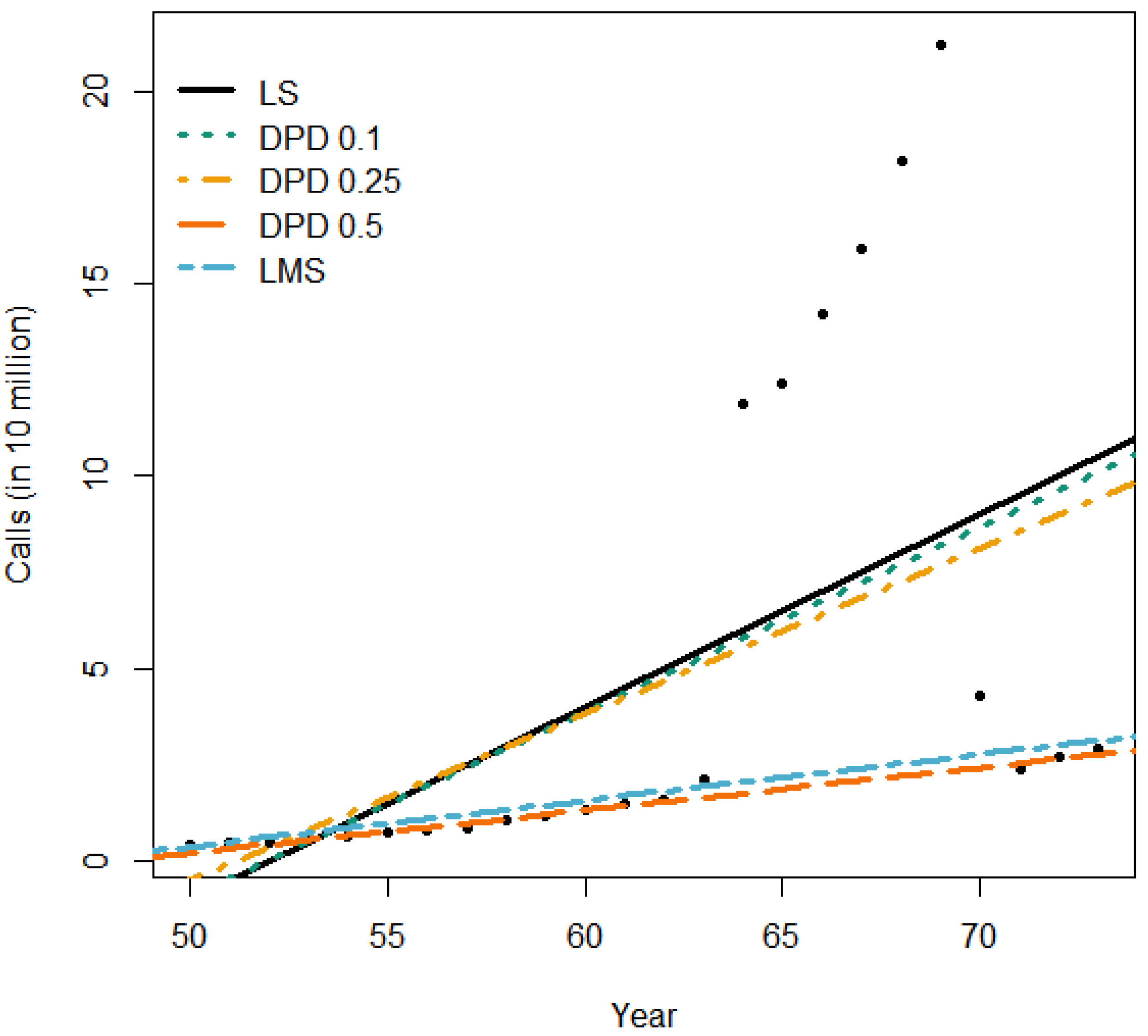
We consider a segment of data obtained from the Belgian Statistical Survey by the Ministry of Economy, Belgium (Table 2, Chap. 2, [27]). Here, the total number (in tens of millions) of international phone calls made in a year is the dependent variable y. The independent variable is the year number x = 50 , 51 , , 73 . However, due to the use of another recording system (giving the total number of minutes of these calls) from the year 1964 to 1969, the data contain heavy contamination in the y-direction in that range. The years 1963 and 1970 are also partially affected for the same reason. Estimates of the linear regression parameters obtained by the minimum DPD and minimum EWD methods are presented in Table A3 and Table A4, respectively.
Table A3. θ ^ for Belgium telephone data using MDPDE(D( α )).
EstimatesD(0)D(0.05)D(0.1)D(0.25)D(0.5)D(1)
Intercept 26.01 25.53 24.94 21.97 5.260 5.360
Slope 0.500 0.500 0.480 0.430 0.110 0.110
Error s.d. 5.380 5.400 5.410 5.290 0.110 0.120
Table A4. θ ^ for Belgium telephone data using MEWDE(E( β )).
EstimatesE(0)E(0.05)E(0.1)E(0.25)E(0.5)E(1)
Intercept 26.010 5.180 5.190 5.180 5.040 5.660
Slope 0.500 0.110 0.110 0.110 0.110 0.120
Error s.d. 5.380 0.090 0.090 0.090 0.080 0.060
We make the following observations based on Figure A3 and Figure A4:
Figure A3. Plots of the data points and fitted regression lines for Belgium telephone data using least squares and minimum DPD estimates.
Mathematics 14 00670 g0a3
Figure A4. Plots of the data points and fitted regression lines for Belgium telephone data using least squares and minimum EWD estimates.
Mathematics 14 00670 g0a4
  • It is clear that the estimators corresponding to α = 0 and β = 0 (which are identical and coincide with the ordinary LS estimators) are heavily affected by the outliers.
  • The MDPDE with α 0.5 are strongly robust with respect to the outliers, giving excellent fits to the remaining observations; while analyzing this dataset, ref. [28] notes that the slope parameter remains practically constant for all α 0.4 .
  • The MEWDE with β 0.05 are strongly robust with respect to the outliers, giving excellent fits to the remaining observations. We note that the estimated regression parameters do not differ by much for all β 0.05 when compared to the outlier-influenced ML regression estimates.
  • The least square estimators of the regression parameters, after deleting the outlying observations corresponding to the years 1964 to 1970 are 5.260 , 0.111 and 0.146 , quite close to all our robust estimators.
Clearly, the performance of the MDPDEs and the MEWDEs are quite competitive in this example.

Appendix B.3. Residual Analysis of Certain Fits for Alcohol Solubility Data

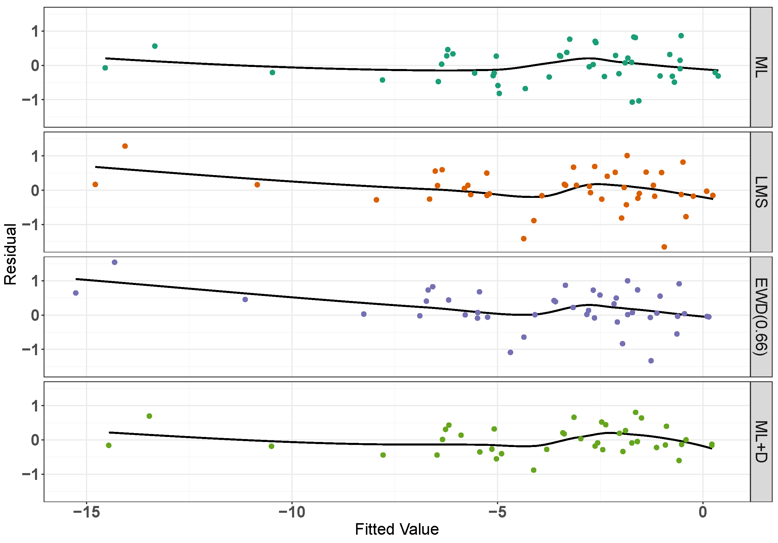
In continuation with the example considered in the main article, we have, in Figure A5, presented the residual plots (against fitted values) of some fits (ML, LMS, ML + D (outlier deleted) and minimum EWD(0.66)) for the alcohol solubility data [25]. In Figure A6, we present the kernel density estimates of the residuals of the same fits.
As noted in the manuscript, we observe that the LMS and minimum EWD(0.66) procedures identify a few outliers. On the other hand, these observations remain masked in the case of the maximum likelihood method, while the ML + D method does not identify any outlier. This is indicated by the lack of the long tails for the ML and ML + D methods.
Figure A5. Scatter plots of the residuals against fitted values for ML, LMS, ML + D and minimum EWD( 0.66 ) fits for alcohol solubility data [25].
Mathematics 14 00670 g0a5
Figure A6. Kernel density estimates of the residuals arising from ML, LMS, ML + D and minimum EWD( 0.66 ) fits for alcohol solubility data [25]. Vertical black lines correspond to 25th, 50 th and 75 th percentiles of corresponding density curves, while red rug-lines correspond to the actual residuals from which the kernel density estimates are obtained.
Mathematics 14 00670 g0a6

Appendix C. Additional Simulation Results

This appendix provides the detailed simulation results for the scenarios referenced in Section 4.4, specifically the estimation of scale in a normal model (Scenario (b)) and the estimation of the mean in an exponential model (Scenario (c)).

Appendix C.1. Estimation of Scale (Standard Deviation)

Table A5 presents the finite sample relative efficiency (FSRE) for estimating the standard deviation σ of a univariate normal distribution N ( 0 , σ 2 ) with a known mean of zero. The data were generated with contamination from a variance-inflated distribution N ( 0 , 3 2 ) . The FSRE is defined as the ratio of the Mean Squared Error (MSE) of the estimator to the MSE of the MLE ( M S E e s t / M S E M L E ). Consequently, values less than 1 indicate that the robust estimator outperforms the MLE. We compare the proposed MEWDE against the MDPDE and two classical robust M-estimators: Huber’s estimator and Tukey’s Bisquare estimator. The columns “MEWDE (Oracle)” and “MDPDE (Oracle)” correspond to the minimum MSE achieved across their respective tuning grids. As shown in Table A5, under pure data ( ϵ = 0 ), the robust estimators exhibit the expected loss of efficiency compared to the MLE (values > 1 ). However, under contamination, the MLE’s performance deteriorates drastically, resulting in low FSRE values for all robust methods. Notably, the MEWDE consistently outperforms the Bisquare estimator and achieves efficiency superior to the Huber estimator across all contaminated scenarios. Furthermore, the MEWDE remains highly competitive with the MDPDE, achieving the lowest MSE in several high-contamination settings (e.g., n = 200 , ϵ = 0.2 ).
Table A5. Finite sample relative efficiency (relative to MLE) for scale estimation ( σ ). Lower values indicate better performance.
n ϵ HuberBisquareMDPDE (Oracle)MEWDE (Oracle)
500.01.7511.9241.1931.198
0.10.2950.2910.1980.218
0.20.1820.3150.1310.129
0.30.1660.3680.1270.126
1000.02.3241.1181.0151.460
0.10.1350.2110.1170.109
0.20.1480.2510.0930.086
0.30.1480.3620.1140.112
2000.02.0531.1151.0311.386
0.10.1140.1690.0810.076
0.20.1010.2420.0770.069
0.30.1460.3630.1090.104

Appendix C.2. Estimation of Exponential Mean

In this scenario, we consider the estimation of the mean parameter θ of an exponential distribution with probability density function f ( x ; θ ) = 1 θ e x / θ , x 0 . The true parameter value was set to θ = 1 . We evaluated the performance of the estimators under sample sizes n { 50 , 100 , 200 } and contamination proportions ϵ { 0.0 , 0.1 , 0.2 , 0.3 } . The contaminated observations were generated from a uniform distribution U ( 20 , 30 ) , representing severe, high-value outliers that typically bias the mean estimate upwards. We compare the proposed MEWDE against the standard MLE (sample mean) and the MDPDE. For the robust benchmark, we utilize the Scaled Median estimator, defined as θ ^ m e d = Median ( X 1 , , X n ) / ln ( 2 ) , which provides a Fisher-consistent and robust estimate for the exponential mean. Unlike the location and scale settings (Scenarios (a) and (b) of simulation 1), we do not include the standard Huber or Tukey’s Bisquare M-estimators in this comparison. These classical estimators are constructed based on symmetric influence functions designed for location-scale families (e.g., the normal distribution). As the exponential distribution is defined on the positive half-line ( [ 0 , ) ) and is highly asymmetric, the direct application of symmetric influence functions is theoretically inappropriate and leads to inconsistent estimates. The Scaled Median serves as the appropriate high-breakdown benchmark for this asymmetric context. Table A6 presents the finite sample relative efficiency (FSRE) of the estimators relative to the MLE. Values less than 1 indicate superior performance compared to the MLE. The results demonstrate that while the MLE breaks down under contamination (resulting in extremely low relative efficiency for the robust methods), the MEWDE consistently outperforms the Scaled Median and achieves parity with the MDPDE.
Table A6. Finite sample relative efficiency (relative to MLE) for Exponential Mean Estimation ( θ ). Lower values indicate better performance.
n ϵ Scaled MedianMDPDE (Oracle)MEWDE (Oracle)
500.01.8551.0021.283
0.10.0130.0060.006
0.20.0140.0030.002
0.30.0750.0090.003
1000.02.4471.0411.564
0.10.0140.0040.004
0.20.0120.0020.002
0.30.0160.0020.002
2000.01.6741.0221.283
0.10.0070.0020.002
0.20.0090.0010.001
0.30.0150.0020.001

Appendix D. Proofs of Theorems

While the proof techniques are inspired by the specific case of the density power divergence in [16,28], the derivations provided in the Appendix D are significantly broader. They establish the asymptotic properties for the entire class of minimum Bregman divergence estimators defined by a general weight function w. As such, these results provide a unified theoretical framework for robust inference in independent non-homogeneous models. Below, we provide the proofs of the asymptotic properties of the minimum Bregman divergence estimator (MBDE) and the associated test statistics. We strictly adopt the notation defined in Section 2, Section 3 and Section 6 of the manuscript.
Recall the objective function for the independent non-homogeneous setting is H n ( θ ) = 1 n i = 1 n V i , θ ( X i ) , where V i , θ ( X i ) is defined in Equation (2). The estimating equation is given by θ H n ( θ ) = S n ( θ ) = 0 , where
S n ( θ ) = 1 n i = 1 n u i , θ ( X i ) w ( f i , θ ( X i ) ) u i , θ ( x ) w ( f i , θ ( x ) ) f i , θ ( x ) d x ,
with w ( t ) = B ( t ) t and u i , θ ( x ) = θ log ( f i , θ ( x ) ) .

Appendix D.1. Proof of Theorem 1

Proof. 
This proof is adapted from [28], generalized here for the Bregman divergence class. We consider the Taylor series expansion of the score function S n ( θ ^ n ) around the true best-fitting parameter θ g . Since θ ^ n is a root of the estimating equation, S n ( θ ^ n ) = 0 . Expanding yields the following:
0 = S n ( θ ^ n ) = S n ( θ g ) + θ S n ( θ n * ) ( θ ^ n θ g ) ,
where θ n * lies on the line segment joining θ ^ n and θ g . Rearranging the terms
n ( θ ^ n θ g ) = [ θ S n ( θ n * ) ] 1 n S n ( θ g ) .
First, we derive the asymptotic distribution of n S n ( θ g ) . Consider n S n ( θ g ) = 1 n i = 1 n θ V i , θ g ( X i ) . Since the observations X i are independent, the terms θ V i , θ g ( X i ) are independent random vectors with mean zero (at the truth θ g ). The covariance matrix is
Var ( n S n ( θ g ) ) = 1 n i = 1 n Var g i [ θ V i , θ g ( X i ) ] = Ω n ,
where Ω n is defined in Equation (11). Under Assumptions 6 and 7 (Lindeberg–Feller conditions), the Central Limit Theorem applies:
Ω n 1 / 2 n S n ( θ g ) d N s ( 0 , I s ) .
Next, we consider the convergence of the Hessian matrix. Consider θ S n ( θ ) = 1 n i = 1 n θ 2 V i , θ ( X i ) . Under Assumptions 1–5 and the Weak Law of Large Numbers for non-homogeneous variables [29,30], θ S n ( θ g ) converges in probability to its expectation:
E [ θ S n ( θ g ) ] = 1 n i = 1 n J ( i ) = Ψ n ,
where J ( i ) is defined in Equation (9) and Ψ n in Equation (10). Given the consistency θ ^ n p θ g , we have θ S n ( θ n * ) p Ψ n . Substituting these results into (A3) provides the following:
n ( θ ^ n θ g ) = Ψ n 1 n S n ( θ g ) + o p ( 1 ) .
Multiplying by Ω n 1 / 2 Ψ n , we obtain the result stated in Theorem 1:
Ω n 1 / 2 Ψ n n ( θ ^ n θ g ) d N s ( 0 , I s ) .

Appendix D.2. Proof of Theorem 2

Proof. 
This proof adapts the logic of [16]. Let the null hypothesis be m ( θ ) = 0 , where m : R s R r is differentiable with Jacobian M ( θ ) = m ( θ ) T θ . The constrained estimator θ ˜ n , B 1 minimizes H n ( θ ) subject to m ( θ ) = 0 . The Lagrangian is L ( θ , λ ) = H n ( θ ) + λ T m ( θ ) . The stationary conditions are
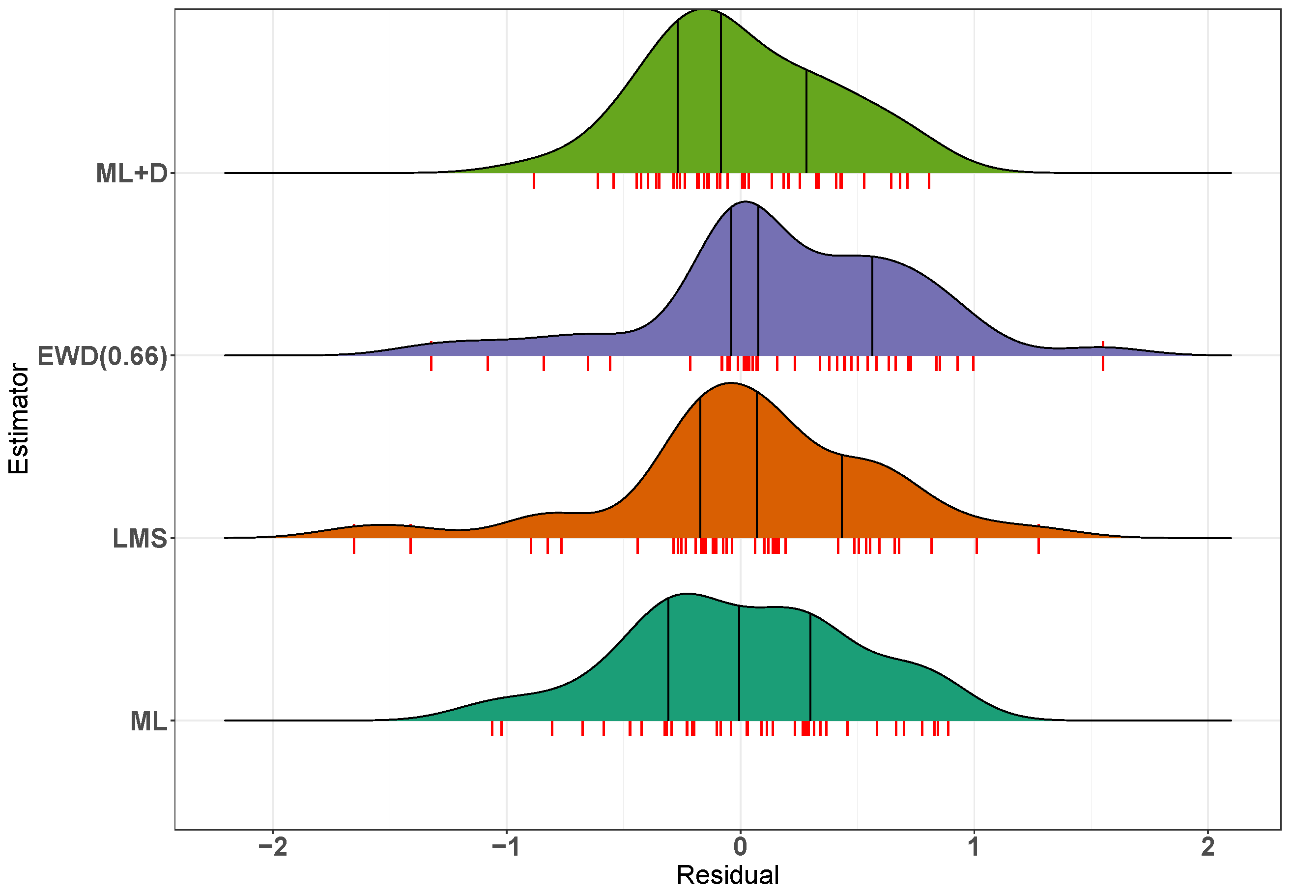
S n ( θ ˜ n , B 1 ) + M ( θ ˜ n , B 1 ) λ ˜ n = 0 ,
m ( θ ˜ n , B 1 ) = 0 .
Expanding (A9) around θ g (where m ( θ g ) = 0 under H 0 ):
S n ( θ g ) + Ψ n ( θ ˜ n , B 1 θ g ) + M ( θ g ) λ ˜ n 0 .
Expanding (A10) around θ g :
m ( θ g ) + M ( θ g ) T ( θ ˜ n , B 1 θ g ) 0 M ( θ g ) T ( θ ˜ n , B 1 θ g ) 0 .
Combining these in matrix form and solving for ( θ ˜ n , B 1 θ g ) :
n ( θ ˜ n , B 1 θ g ) n P Ψ n Ψ n 1 S n ( θ g ) ,
where P Ψ n = I s Ψ n 1 M ( θ g ) [ M ( θ g ) T Ψ n 1 M ( θ g ) ] 1 M ( θ g ) T . This can be rewritten using the notation P B 1 from Theorem 2 (assuming B 1 is the divergence used):
n ( θ ˜ n , B 1 θ g ) P B 1 Ψ n n Ψ n 1 S n ( θ g ) .
Since n S n ( θ g ) d N ( 0 , Ω n ) , the asymptotic distribution is normal with covariance matrix Σ B 1 = P B 1 Ψ n ( Ψ n 1 Ω n Ψ n 1 ) Ψ n P B 1 T = P B 1 Ω n P B 1 T . □

Appendix D.3. Proof of Theorem 3

Proof. 
Let the test statistic be T B 2 = 2 n D B 2 ( f θ ^ n , f θ ˜ n ) . Under H 0 , a second-order Taylor expansion of the divergence around θ ^ n gives
T B 2 n ( θ ^ n θ ˜ n ) T A B 2 ( θ g ) ( θ ^ n θ ˜ n ) ,
where A B 2 ( θ g ) corresponds to the Hessian of the divergence D B 2 . Using the expansions from Theorems 1 and 2,
n ( θ ^ n θ g ) Ψ n 1 n S n ( θ g ) ,
n ( θ ˜ n θ g ) P B 1 n S n ( θ g ) Ψ n 1 .
The difference is n ( θ ^ n θ ˜ n ) ( Ψ n 1 P B 1 Ψ n 1 ) n S n ( θ g ) . This simplifies using the definition of Q in Theorem 2 ( P B 1 = Ψ n 1 Q M Ψ n 1 ) to
n ( θ ^ n θ ˜ n ) Q n S n ( θ g ) .
Substituting back into the quadratic form:
T B 2 [ n S n ( θ g ) ] T Q T A B 2 Q [ n S n ( θ g ) ] .
Since n S n ( θ g ) N ( 0 , Ω n ) , we can write n S n ( θ g ) = Ω n 1 / 2 Z where Z N ( 0 , I ) .
T B 2 Z T ( Ω n 1 / 2 Q T A B 2 Q Ω n 1 / 2 ) Z .
This is a quadratic form Z T M n Z . Its distribution is λ i Z i 2 , where λ i are the eigenvalues of M n , or equivalently, the non-zero eigenvalues of A B 2 Q Ω n Q . Identifying B B 1 from Theorem 3 with components of Q, we obtain the result in Equation (21). □

References

  1. Csiszár, I. Eine informationstheoretische ungleichung und ihre anwendung auf beweis der ergodizitaet von markoffschen ketten. Magyer Tud. Akad. Mat. Kut. Int. Koezl. 1963, 8, 85–108. [Google Scholar]
  2. Lindsay, B.G. Efficiency versus robustness: The case for minimum Hellinger distance and related methods. Ann. Stat. 1994, 22, 1081–1114. [Google Scholar] [CrossRef]
  3. Beran, R. Minimum Hellinger distance estimates for parametric models. Ann. Stat. 1977, 5, 445–463. [Google Scholar] [CrossRef]
  4. Basu, A.; Shioya, H.; Park, C. Statistical Inference: The Minimum Distance Approach; Chapman and Hall/CRC: Boca Raton, FL, USA, 2011. [Google Scholar]
  5. Simpson, D.G. Hellinger deviance tests: Efficiency, breakdown points, and examples. J. Am. Stat. Assoc. 1989, 84, 107–113. [Google Scholar] [CrossRef]
  6. Basu, A.; Harris, I.R.; Hjort, N.L.; Jones, M. Robust and efficient estimation by minimising a density power divergence. Biometrika 1998, 85, 549–559. [Google Scholar] [CrossRef]
  7. Broniatowski, M.; Toma, A.; Vajda, I. Decomposable pseudodistances and applications in statistical estimation. J. Stat. Plan. Inference 2012, 142, 2574–2585. [Google Scholar] [CrossRef][Green Version]
  8. Jana, S.; Basu, A. A characterization of all single-integral, non-kernel divergence estimators. IEEE Trans. Inf. Theory 2019, 65, 7976–7984. [Google Scholar] [CrossRef]
  9. Si, T.; Wang, Y.; Zhang, L.; Richmond, E.; Ahn, T.H.; Gong, H. Multivariate time series change-point detection with a novel Pearson-like scaled Bregman divergence. Stats 2024, 7, 462–480. [Google Scholar] [CrossRef]
  10. Wang, Y.; Zhang, L.; Si, T.; Bishop, G.; Gong, H. Anomaly Detection in High-Dimensional Time Series Data with Scaled Bregman Divergence. Algorithms 2025, 18, 62. [Google Scholar] [CrossRef]
  11. Duan, X.; Mu, A.; Zhao, X.; Wu, Y. A K-Means Clustering Algorithm with Total Bregman Divergence for Point Cloud Denoising. Symmetry 2025, 17, 1186. [Google Scholar] [CrossRef]
  12. Omanwar, A.; Alajaji, F.; Linder, T. Bounds on the Excess Minimum Risk via Generalized Information Divergence Measures. Entropy 2025, 27, 727. [Google Scholar] [CrossRef] [PubMed]
  13. Ardakani, O.M. Robust Learning of Tail Dependence. Econometrics 2025, 13, 47. [Google Scholar] [CrossRef]
  14. Pardo, L. Statistical Inference Based on Divergence Measures; CRC Press: Boca Raton, FL, USA, 2006. [Google Scholar]
  15. Basu, A.; Mandal, A.; Martin, N.; Pardo, L. Testing statistical hypotheses based on the density power divergence. Ann. Inst. Stat. Math. 2013, 65, 319–348. [Google Scholar] [CrossRef]
  16. Basu, A.; Mandal, A.; Martin, N.; Pardo, L. Testing Composite Hypothesis Based on the Density Power Divergence. Sankhya B 2018, 80, 222–262. [Google Scholar] [CrossRef]
  17. Csiszár, I. Why least squares and maximum entropy? An axiomatic approach to inference for linear inverse problems. Ann. Stat. 1991, 19, 2032–2066. [Google Scholar] [CrossRef]
  18. Feller, W. An Introduction to Probability Theory and Its Applications; Wiley: New York, NY, USA, 1971; Volume 963. [Google Scholar]
  19. Warwick, J.; Jones, M. Choosing a robustness tuning parameter. J. Stat. Comput. Simul. 2005, 75, 581–588. [Google Scholar] [CrossRef]
  20. Soetaert, K. rootSolve: Nonlinear Root Finding, Equilibrium and Steady-State Analysis of Ordinary Differential Equations; R package 1.6; R Foundation for Statistical Computing: Vienna, Austria, 2009. [Google Scholar]
  21. Hettmansperger, T.P.; McKean, J.W. Robust Nonparametric Statistical Methods; CRC Press: Boca Raton, FL, USA, 2010. [Google Scholar]
  22. Woodruff, R.; Mason, J.; Valencia, R.; Zimmering, S. Chemical mutagenesis testing in Drosophila: I. Comparison of positive and negative control data for sex-linked recessive lethal mutations and reciprocal translocations in three laboratories. Environ. Mutagen. 1984, 6, 189–202. [Google Scholar] [CrossRef] [PubMed]
  23. Roser, M.; Ritchie, H. Homicides. Our World in Data. 2020. Available online: https://ourworldindata.org/homicides (accessed on 2 February 2026).
  24. Central Intelligence Agency. CIA World Factbook 2022–2023; Simon and Schuster: New York, NY, USA, 2022. [Google Scholar]
  25. Maronna, R.A.; Martin, R.D.; Yohai, V.J.; Salibián-Barrera, M. Robust Statistics: Theory and Methods (with R); John Wiley & Sons: Hoboken, NJ, USA, 2019. [Google Scholar]
  26. Basak, S.; Basu, A.; Jones, M. On the ‘optimal’ density power divergence tuning parameter. J. Appl. Stat. 2020, 48, 536–556. [Google Scholar] [CrossRef] [PubMed]
  27. Rousseeuw, P.J.; Leroy, A.M. Robust Regression and Outlier Detection; Wiley Online Library: Hoboken, NJ, USA, 1987; Volume 1. [Google Scholar]
  28. Ghosh, A.; Basu, A. Robust estimation for independent non-homogeneous observations using density power divergence with applications to linear regression. Electron. J. Stat. 2013, 7, 2420–2456. [Google Scholar] [CrossRef]
  29. Van der Vaart, A.W. Asymptotic Statistics; Cambridge University Press: Cambridge, UK, 2000; Volume 3. [Google Scholar]
  30. White, H. Asymptotic Theory for Econometricians; Academic Press: Amsterdam, The Netherlands, 2014. [Google Scholar]
Figure 1. Weight functions of some DPD( α ) members.
Mathematics 14 00670 g001
Figure 2. Weight functions of some EWD( β ) members.
Mathematics 14 00670 g002
Figure 3. Influence function for μ ^ from the contaminated normal distribution ( 1 ϵ ) N ( μ , 1 ) + ϵ Δ t for some MEWDE( β ).
Mathematics 14 00670 g003
Figure 5. Analysis of the Shoshoni dataset. The plot overlays the estimated density curves for MLE, Huber, Bisquare, MDPDE ( α = 0.5 ), and MEWDE ( β = 0.4 ) on the data points.
Mathematics 14 00670 g005
Figure 6. Histogram of Drosophila count data (truncated at x = 8 ) with overlaid Poisson density estimates using MLE, MLE + D, MDPDE (0.50), MEWDE (0.25), and L 2 .
Mathematics 14 00670 g006
Figure 7. Modeling firearm-related homicide rates in Western countries as a function of per-capita gross domestic product: fits with MLE, MLE + D, MEWDE, MDPDE, Huber, and Bisquare estimators.
Mathematics 14 00670 g007
Figure 8. Power curves of the proposed robust Wald-type test for varying sample sizes (n) and contamination levels ( ϵ ).
Mathematics 14 00670 g008
Figure 9. p-value of EWDTS( β ) for β > 0 for the Shoshoni rectangles dataset.
Mathematics 14 00670 g009
Table 1. Finite sample relative efficiency (FSRE) of the MEWDE compared to the MLE and MDPDE under varying contamination levels ( ϵ ) and sample sizes (n).
ϵ nRelative Efficiency
HuberBisquareMDPDE (Oracle)MEWDE (Oracle)
0.0501.0211.0451.0021.012
1001.0021.0131.0061.004
2001.0351.0551.0441.003
0.1500.3150.1230.0870.078
1000.2630.0650.0470.039
2000.2310.0400.0300.024
0.2500.6780.4040.2610.027
1000.5820.2650.0230.016
2000.5550.2000.0140.008
0.3500.9200.7920.3956.413
1000.9180.7880.0930.995
2000.9230.8040.0140.005
Table 2. Comparison of Mean Squared Error (MSE) between the Oracle-tuned MEWDE and the data-driven MEWDE (using the Warwick–Jones algorithm with minimum L 2 pilot).
ϵ nMSE (Oracle)MSE (Data-Driven)% Loss
0.00250.04920.061224.41%
1000.01250.015524.06%
5000.00230.002719.31%
0.05251.12441.18935.78%
1000.55930.56220.53%
5000.25820.25910.34%
0.10251.35991.37461.08%
1002.07942.08430.23%
5001.71921.71950.02%
0.20251.71201.77913.92%
1004.29754.29980.05%
5009.41439.41450.00%
Table 3. Parameter estimation error (sum of squared errors, β ^ β 2 2 ) for multivariate linear regression with p predictors. Data were generated with 10% and 20% vertical outliers from N ( 20 , 1 ) .
ϵ npMLEMEWDE
β = 0 . 1 β = 0 . 5
0.05020.0450.0570.069
10050.0540.0710.091
50100.2530.4130.606
100100.1110.1560.209
200100.0530.0670.082
0.15021.6750.0570.066
10052.2870.0680.079
501010.4350.4180.592
200102.1680.0700.082
0.25023.4180.0560.063
10054.2180.0750.084
501020.5550.4060.518
200104.4000.0720.080
Table 4. Parameter estimates for the Shoshoni dataset using classical and robust estimators. N ( μ , σ 2 ) distribution is fitted using MLE, Huber, Bisquare, MDPDE ( α = 0.5 ), and MEWDE ( α = 0.4 ).
Method μ ^ σ ^
MLE0.66050.0902
Huber0.64210.0519
Bisquare0.63450.0519
MDPDE ( α = 0.5 )0.63140.0472
MEWDE ( α = 0.4 )0.60600.0421
Table 5. Fitted frequencies for Drosophila data using MLE, MDPDE (denoted by D( α )) and MEWDE (denoted by E( β )), where α and β are tuning parameters for MDPDE and MEWDE.
Count01234≥5 λ ^
Observed2373001 (91)
MLE. 1.596 4.882 7.467 7.613 5.822 6.620 3.059
D( 0.10 ) 22.981 9.002 1.763 0.230 0.023 0.002 0.392
D( 0.50 ) 23.375 8.759 1.641 0.205 0.019 0.002 0.375
D( 0.75 ) 23.549 8.649 1.588 0.194 0.018 0.001 0.367
E( 0.001 ) 22.894 9.055 1.791 0.236 0.023 0.002 0.396
E( 0.02 ) 22.614 9.222 1.880 0.256 0.026 0.002 0.408
E( 0.25 ) 23.712 8.545 1.540 0.185 0.017 0.001 0.360
L 2 23.609 8.611 1.570 0.191 0.017 0.001 0.365
MLE + D 22.93 9.03 1.78 0.23 0.02 0 0.39
Table 6. Regression coefficient estimates and scale estimates for the homicide rate dataset. The response variable is the homicide rate, and the predictor is GDP.
ParameterMLEML + DHuberBisquareMEWDE (0.3)MEWDE (0.5)MDPDE (0.3)MDPDE (0.5)
Intercept ( β 0 )−0.2930.3560.3330.3570.3480.3510.3600.364
Slope ( β 1 × 10 5 )1.45−0.30−0.25−0.31−0.31−0.32−0.32−0.33
Sigma ( σ )0.9590.1160.1150.1120.1020.1030.1090.108
Table 7. Estimated regression parameters for alcohol solubility data.
EstimatesMLELMSE(0.1)E(0.4)E(0.7)HuberBisquare
Intercept 8.777 3.617 5.883 3.974 5.444 7.9907.919
SAG 0.014 0.177 0.110 0.163 0.129 0.038 0.041
Volume 0.040 0.191 0.133 0.179 0.152 0.063 0.066
Mass 0.027 0.248 0.172 0.235 0.206 0.063 0.068
Error s.d. 0.504 0.405 0.372 0.145 0.221 0.541 0.552
Disclaimer/Publisher’s Note: The statements, opinions and data contained in all publications are solely those of the individual author(s) and contributor(s) and not of MDPI and/or the editor(s). MDPI and/or the editor(s) disclaim responsibility for any injury to people or property resulting from any ideas, methods, instructions or products referred to in the content.