GPU-Based Parallel Euclidean Distance Transform Algorithm

Abstract

Euclidean distance transform (EDT) often suffers from high computational complexity and limited processing efficiency, especially when applied to large-scale images. To address these challenges, this paper proposes a GPU-based parallel EDT algorithm. The proposed approach first partitions the input image into multiple horizontal sub-blocks. For each sub-block, a row-wise recursive computation strategy is adopted to construct its Voronoi diagram in parallel, thereby reducing computational overhead by exploiting the strong structural similarity between the Voronoi diagrams of adjacent rows. Based on the Voronoi diagrams of all sub-blocks, the Euclidean distance from each pixel to the nearest background pixel is subsequently evaluated, completing the transform. Experimental results demonstrate that the proposed algorithm achieves up to a 52× speedup over traditional CPU-based EDT methods, leading to a substantial improvement in computational performance. Nevertheless, the scalability of the method is influenced by GPU memory capacity and the chosen sub-block partitioning strategy when processing extremely large images. Moreover, the core idea of leveraging inter-row Voronoi similarity to reduce redundant computation can be naturally extended to higher-dimensional exact EDT as well as approximate EDT variants.

1. Introduction

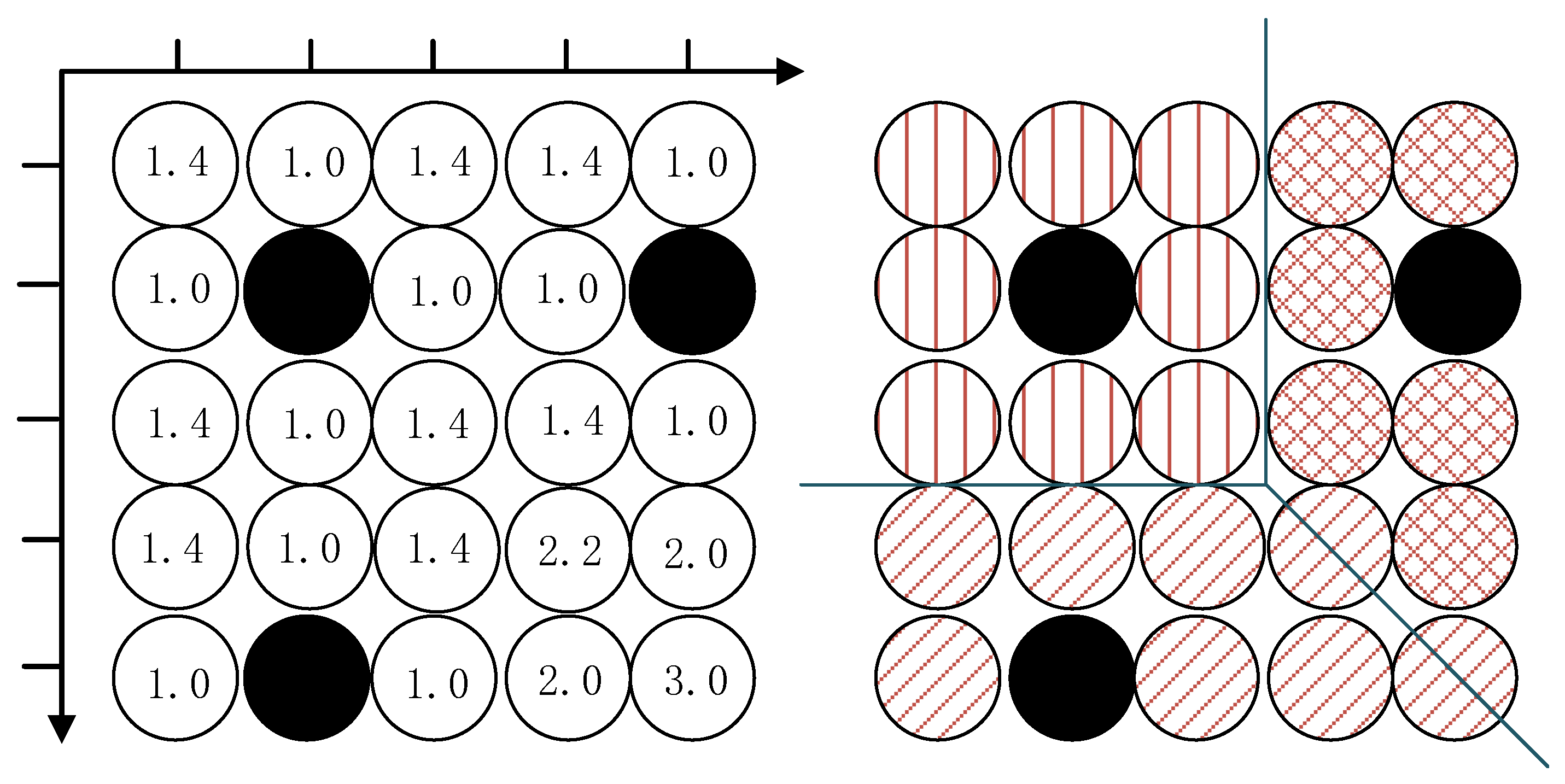
The Euclidean distance transform (EDT) is a fundamental operation in image processing and computer vision, and is widely used in applications such as shape analysis, object segmentation, and medial axis extraction. Given a binary image, EDT computes the shortest Euclidean distance from each foreground pixel to its nearest background pixel, thereby producing a Euclidean distance map that supports various high-level vision tasks. During this process, the image is typically represented as a matrix composed of discrete pixels, where each pixel can be regarded as a point in a two-dimensional space whose coordinates are determined by its column and row indices. This representation allows direct computation of Euclidean distances between pixels and facilitates the application of computational geometry techniques—such as Voronoi diagrams and convex hulls—to optimize distance transform algorithms and improve both computational efficiency and accuracy. As illustrated on the left side of Figure 1, a $5\times 5$ binary image is embedded in a two-dimensional coordinate system, where black-filled circles denote background pixels and white-filled circles represent foreground pixels. The numerical values inside the circles indicate the Euclidean distance from each foreground pixel to its nearest background pixel.

The Voronoi diagram is a classical spatial partitioning structure that has been extensively studied and applied in computational geometry, image processing, geographic information systems, and machine learning. In the context of EDT, the Voronoi diagram provides a clear geometric interpretation of the nearest-background-pixel assignment problem. Specifically, given a set of background pixels, the image domain is partitioned into a collection of Voronoi cells, each of which is associated with a unique background pixel. Each Voronoi cell consists of all foreground pixels whose Euclidean distance to its associated background pixel is smaller than that to any other background pixel. Consequently, for any foreground pixel within a given Voronoi cell, the associated background pixel is guaranteed to be its nearest background pixel, and their Euclidean distance directly yields the EDT value. This formulation enables an efficient and structured computation of the distance transform and serves as a foundation for parallel EDT algorithms, since distance calculations for all foreground pixels can be performed independently and simultaneously.

On the left side of Figure 1, three background pixels are present. Accordingly, the Voronoi diagram shown on the right partitions the entire image into three distinct regions, each corresponding to a different background pixel and delineated by a unique background pattern. For a two-dimensional image, the Voronoi diagram can be computed either in a single global pass or by decomposing the image into multiple sub-blocks that are processed independently, after which the resulting partial diagrams are merged to obtain the complete diagram. Following this strategy, the Voronoi diagram of a sub-block is constructed by further decomposing it into individual image rows. The Voronoi diagram of each row is computed independently and then aggregated to form the Voronoi diagram of the entire sub-block. Because adjacent image rows typically exhibit strong structural similarity in their Voronoi diagrams, the diagram of a given row can be efficiently derived from that of its neighboring row through recursive updates, rather than being recomputed from scratch. This approach significantly reduces redundant computations and lowers the overall computational cost.

Modern NVIDIA graphics processing units (GPUs) adopt a programmable many-core architecture with a hierarchical organization of parallel computing resources. Each GPU consists of multiple Streaming Multiprocessors (SMs), and each SM contains dozens of stream processors, along with a large register file and a capacity-limited but low-latency shared memory. In addition, GPUs provide a global memory space that is accessible by all SMs through a high-bandwidth interconnect. CUDA programs expose massive parallelism via a hierarchical execution model composed of grids and thread blocks, while a hardware scheduler dynamically assigns thread blocks to available SMs to maximize resource utilization. Owing to their fine-grained parallelism and the ability to execute tens of thousands of concurrent threads, GPUs can accelerate traditionally serial algorithms by one to two orders of magnitude, offering substantial performance gains for high-performance computing applications.

As image resolutions and data dimensionalities continue to increase, traditional serial EDT algorithms can no longer satisfy the demands of efficient processing. Consequently, both computation time and resource consumption have become major bottlenecks in practical applications. Although previous studies have explored parallel approaches to accelerate EDT, the strong data dependencies and irregular memory-access patterns inherent to the problem significantly limit the performance gains achievable on GPUs. To overcome these challenges, this work investigates GPU-oriented parallel computing techniques, focusing on two key objectives: (1) designing data-partitioning and scheduling strategies that effectively exploit GPU parallelism, and (2) substantially reducing overall computational cost while preserving scalability.

In this paper, we propose an efficient GPU-based parallel algorithm for computing the Euclidean distance transform. The proposed method integrates a task-partitioning strategy that combines row-wise decomposition with Voronoi-based spatial decomposition, and introduces an incremental update mechanism that significantly enhances parallelism while reducing computational complexity, without sacrificing accuracy. The core contribution lies in leveraging Voronoi diagrams for data partitioning to maximize parallel execution, while relaxing the conventional assumption in traditional Voronoi-intersection methods that each image row must be processed independently. By fully exploiting the structural similarity between the Voronoi diagrams of adjacent rows, the proposed algorithm eliminates redundant computation and further improves parallel efficiency, providing an effective solution for accelerating EDT in large-scale image-processing applications.

2. Related Work

This section focuses on the discussion of two-dimensional exact EDT algorithms. Three-dimensional or approximate EDT algorithms are beyond the scope of this study.

2.1. Serial Algorithms

Based on the order in which pixels are processed, the serial EDT algorithms can generally be classified into three categories [1,2]: raster-scanning algorithms [3,4,5], propagation algorithms [6,7], and independent-scanning algorithms [8,9]. Raster-scanning algorithms start from the top-left corner of the image and traverse pixels from left to right and from top to bottom, using a two-dimensional mask to estimate the distance from each pixel to its nearest background pixel. A reverse scan is subsequently performed from the bottom-right corner, proceeding from right to left and from bottom to top, during which distance values are refined using the same update scheme. Propagation algorithms treat each background pixel as a seed and iteratively propagate distance information to neighboring foreground pixels. Through this iterative process, the distance from every foreground pixel to its nearest background pixel is eventually determined. Independent-scanning algorithms adopt a dimensionality-reduction strategy and typically operate in two stages. In the first stage, distance information is computed independently along the column direction. In the second stage, each row independently determines the distance from its foreground pixels to their nearest background pixels based on the intermediate results produced in the first stage, without introducing inter-row dependencies. Depending on the specific implementation of the second stage, independent-scanning algorithms can be further divided into three groups: parabolic-intersection–based methods [10], mathematical-morphology–based methods [11], and Voronoi-diagram-intersection–based methods [12].

In addition to these categories, Silva et al. [13] proposed a component-tree–based approach for computing the maximal distance transform, while Ali et al. [14] introduced a voxel-accelerated data structure that efficiently maintains and queries EDT results.

2.2. Parallel Algorithms

The optimal serial EDT algorithm has a time complexity of $O\left(n^2\right)$ [12]. However, for large-scale images, the associated computational cost becomes prohibitively high, severely constraining overall efficiency. As a result, the development of efficient parallel EDT algorithms—particularly those targeting GPU architectures—has become increasingly important.

Raster-scanning algorithms are inherently difficult to parallelize because their strict sequential processing order limits opportunities for effective parallel execution. In [15], the image is partitioned into multiple regions, each assigned to a thread block, and these regions are further subdivided into smaller subregions in which individual threads perform raster scanning. Nevertheless, this approach achieves less than a fourfold speedup over the serial implementation, indicating limited parallel efficiency. In [16], the raster-scanning algorithm from [17] is ported to the GPU and reported to achieve substantial acceleration; however, the work provides neither a detailed description of the parallelization strategy nor sufficient experimental evidence, raising concerns regarding reproducibility and scientific rigor.

The performance of propagation algorithms largely depends on the data structures used to manage pixels awaiting propagation, such as priority queues [18] or bucket-based schemes. The degree to which these data structures can be parallelized directly affects the overall efficiency of the algorithm. However, implementing highly optimized parallel versions of such structures on GPUs or multicore processors remains challenging [19]. Moreover, parallel propagation algorithms [20,21] may introduce small numerical errors, making them more suitable for approximate EDT computations rather than exact transforms.

For these reasons, most parallel EDT algorithms adopt the independent-scanning paradigm. Zampirolli et al. [22] parallelized the mathematical-morphology–based approach proposed in [11] and implemented it on GPUs; however, the resulting computational efficiency remains limited. Cao et al. [23] proposed a parallel EDT algorithm based on the Voronoi-diagram-intersection method. To increase parallelism, each image row is divided into multiple segments, and individual threads independently compute local Voronoi diagrams, which are subsequently merged to form the complete diagram for the row. Man et al. [24,25,26] focused on parallelizing the serial Voronoi-diagram-intersection algorithm originally proposed by Breu et al. [27]. In this approach, parallelism is expressed at the image-row level: each image row is assigned to a group of GPU threads, and the Voronoi diagram construction for different rows is carried out independently and concurrently. This row-wise independence naturally maps to GPU thread-level parallelism and does not require inter-row synchronization.

More recently, Chen et al. [28] proposed a GPU-accelerated incremental EDT method for online motion planning, while Black et al. [29] introduced a hardware-agnostic GPU acceleration framework for EDT computation with multi-threading and cross-language support. In addition, Gallet et al. [30] investigated the use of Tensor Cores (matrix multiply–accumulate units) to accelerate double-precision Euclidean distance computations. Zhu et al. [31] proposed VDB-EDT, an efficient Euclidean distance transform algorithm that leverages the VDB sparse volumetric data structure to represent distance fields hierarchically. The algorithm optimizes scheduling priorities within the transform procedure to accelerate running speed. Han et al. [32] presents a dedicated parallel hardware architecture that exploits the separability of the Euclidean distance transform to achieve high-throughput EDT computation on binary images, particularly suited for FPGA-based real-time processing.

The proposed parallel EDT algorithm falls into the category of independent-scanning algorithms. Compared with classical independent-scanning algorithms [24,25,26,29], the proposed EDT algorithm differs in that it exploits inter-row similarity through a partition-based recursive strategy. Instead of constructing the Voronoi diagram of each row independently, the algorithm reuses proximate-point information across rows within a sub-block, which significantly reduces redundant computations while preserving exact EDT results.

3. Parallel Euclidean Distance Transform Algorithm

3.1. Overview

In a binary image, drawing the perpendicular bisectors of the line segments connecting adjacent background pixels partitions the image plane into a collection of polygons, known as Voronoi cells. Together, these cells form the Voronoi diagram of the image. By definition, each Voronoi cell is associated with the background pixel that is closest to all foreground pixels within that region. Consequently, the distance from any foreground pixel to its associated background pixel corresponds exactly to the Euclidean distance required by EDT. Although this property of the Voronoi diagram is highly advantageous for EDT computation, explicitly constructing the complete Voronoi diagram for an entire image incurs substantial computational cost and therefore impractical for many real-world engineering applications.

To address this challenge, we adopt a block-wise strategy in which the input image is horizontally partitioned into multiple sub-blocks, and the Voronoi diagram within each sub-block is computed independently. The complete Voronoi diagram of the entire image is then obtained by aggregating the local Voronoi diagrams generated from all sub-blocks. Within each sub-block, the problem is reduced to constructing the Voronoi diagram for each individual image row. The Voronoi diagram of an arbitrary row can be interpreted as the intersection between the global Voronoi diagram and that row. Equivalently, each Voronoi cell appearing on a row corresponds to a one-dimensional slice of the global Voronoi diagram restricted to that row, thereby reflecting the local spatial partitioning induced by the global geometric structure.

Given that each image row contains n pixels, it can intersect with at most $O\left(n\right)$ Voronoi cells, each of which corresponds to a distinct background pixel. Equivalently, the Voronoi diagram of a row is fully determined by a set of $O\left(n\right)$ background pixels [27], referred to as the proximate points of that row. Consequently, the Voronoi diagram of a row and its corresponding proximate-point set provide equivalent representations. Moreover, the similarity between two image rows can be quantitatively characterized by the differences between their respective proximate-point sets.

Neighboring image rows often exhibit highly similar Voronoi structures. Motivated by this observation, our method employs an incremental update mechanism that constructs the proximate-point set of each row by updating that of its predecessor, rather than recomputing it from scratch. Specifically, when processing a new row, proximate points that are no longer geometrically valid are removed, while newly relevant points inherited from the previous row are inserted. This incremental strategy preserves the correctness of the Voronoi representation while eliminating redundant computations. As a result, the overall computational workload is substantially reduced, leading to a more efficient Euclidean distance transform that is well suited for large-scale images and GPU-accelerated execution.

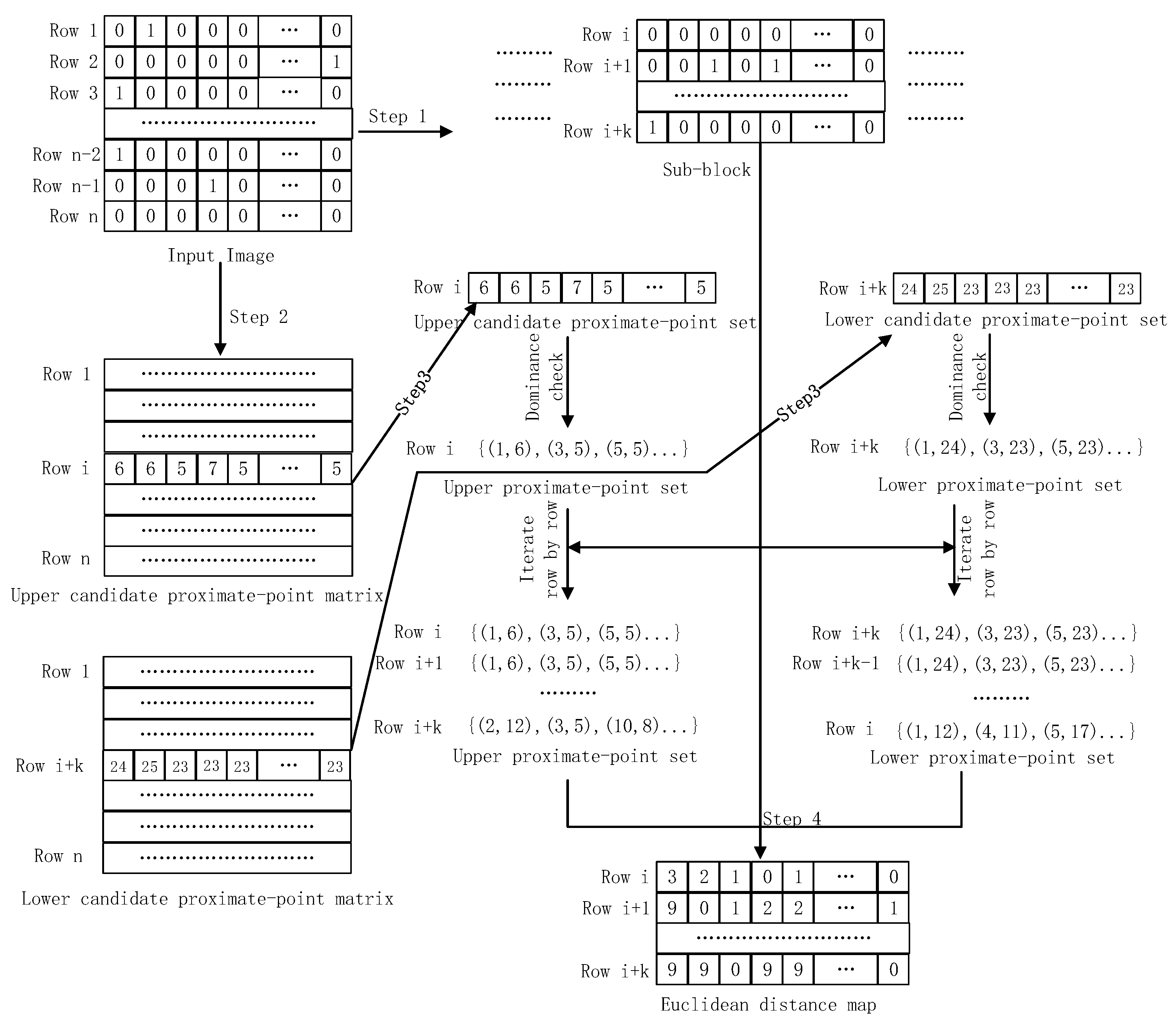
Figure 2 illustrates the overall workflow of the proposed algorithm, which consists of four main steps:

• Partitioning: The input image is horizontally divided into k sub-blocks, denoted as $S_1$, $S_2$, …, $S_k$. The input image in Figure 2 uses 0 and 1 to represent foreground and background pixels, respectively. The example sub-block contains a contiguous set of rows, ranging from row i to row $i+k$.
• Candidate Proximate-point Matrix Computation: An upper candidate proximate-point matrix and a lower candidate proximate-point matrix are constructed via row-wise forward propagation and row-wise backward propagation. Each row of these matrices stores the upper or lower candidate proximate-point set corresponding to that image row.
• Proximate-point Set Computation: The upper and lower proximate-point sets for all rows within each sub-block are generated using a row-wise recursive strategy. In illustrated in Figure 2, the upper proximate-point set of row i is obtained by eliminating dominated candidate proximate points through a dominance check on the upper candidate proximate-point set of that row. Subsequently, a row-wise recurrence is performed from row i to row $i+k$ to compute the upper proximate-point sets for rows i to $i+k$. An analogous procedure is applied in the reverse direction, from row $i+k$ to row i, to compute the lower proximate-point set.
• Euclidean Distance Computation: Based on the upper and lower proximate-point set of all rows in the sub-block, the nearest background pixel for each foreground pixel is determined, and the corresponding Euclidean distance is calculated, thereby producing the Euclidean distance map of the sub-block.

The remainder of this section provides a detailed description of Steps 2, 3, and 4.

Figure 2. Algorithm flowchart.

Figure 2. Algorithm flowchart.

3.2. Computation of the Upper and Lower Candidate Proximate-Point Matrices

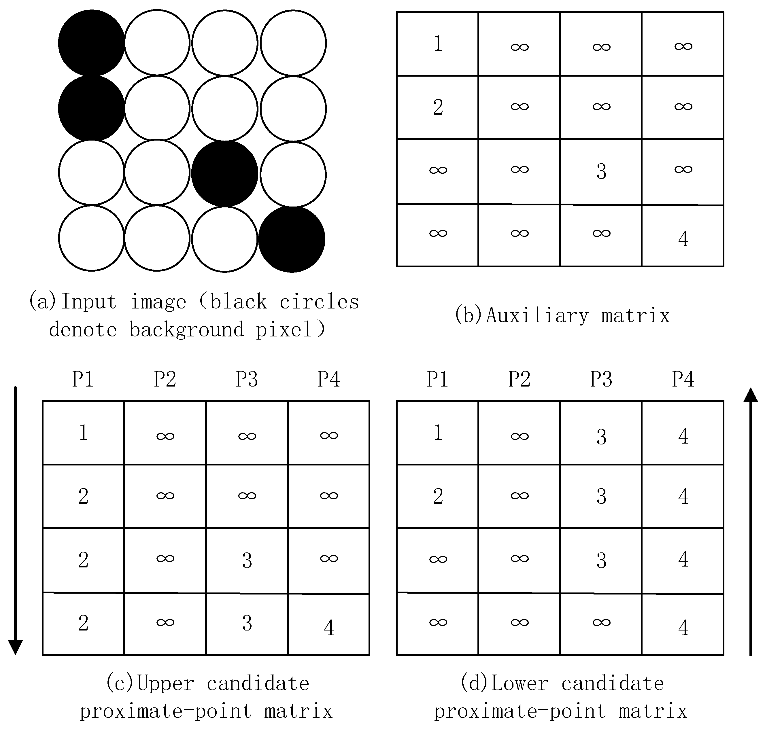
For any pixel in an image row, its upper candidate proximate point is defined as the nearest background pixel located in the same column above it, whereas its lower candidate proximate point is the nearest background pixel located in the same column below it. Consequently, for a row consisting of n pixels, both the upper and lower candidate proximate-point sets contain exactly n elements. From the definition of a candidate proximate point, the candidate proximate-point set for a row can be seen as a superset of the proximate-point set. Figure 3 illustrates the procedure for computing the matrices that stores these candidate proximate-point sets for all rows.

We first extract the background-pixel information from the input image (Figure 3a) and initialize an auxiliary matrix with the same dimensions as the original image (Figure 3b). In this matrix, each entry is assigned the row index of the corresponding pixel if it is a background pixel, and $+\infty$ otherwise. This auxiliary matrix serves as the input for computing the upper and lower candidate proximate-point matrices for all image rows.

To obtain the upper candidate proximate-point matrix, a row-wise forward propagation is performed from top to bottom. Starting from the first row, each entry in the current row is compared with the corresponding entry in the next row. If the value in the next row is $+\infty$, it is replaced by the value from the current row; otherwise, the original value is retained. After completing this propagation, the resulting matrix (Figure 3c) records, for each pixel, the row index of its upper candidate proximate point. Consequently, each row of this matrix corresponds to the upper candidate proximate-point set of the associated image row.

An important observation is that all column-wise operations within a row are mutually independent. Therefore, each pixel can be mapped to an individual GPU thread, enabling the forward propagation to be executed in a highly parallel manner.

The lower candidate proximate-point matrix (Figure 3d) is computed in an analogous manner. Starting from the last row of the auxiliary matrix, a backward propagation is performed from bottom to top. At each step, the current row is compared with the row above it, and entries with infinite values are updated accordingly. Through this process, the nearest background pixel located below each pixel is identified, thereby generating the lower candidate proximate-point matrix as well as the corresponding lower candidate proximate-point set for every image row.

3.3. Computation of the Upper and Lower Proximate-Point Sets

The Voronoi diagram of each sub-block is constructed from the Voronoi diagrams of all image rows within that sub-block. For each row, its proximate-point set can be independently extracted from the candidate proximate-points set in $O\left(n\right)$ time using the method described in [27]. However, because proximate-point sets of adjacent rows typically exhibit strong structural similarity—especially in images with sparsely distributed background pixels—this property can be exploited through a recursive update strategy to avoid redundant computations and thereby further improve overall efficiency.

To efficiently construct the Voronoi diagram of each row, we design a two-stage recursive procedure consisting of a top-down pass followed by a bottom-up pass. To support these passes, the proximate-point set introduced in Section 3.1 is further decomposed into two subsets: the upper proximate-point set and the lower proximate-point set. For any given row, the upper proximate-point set contains the $O\left(n\right)$ background pixels that determine the row’s Voronoi diagram when only the background pixels in the current row and all rows above it are considered. Similarly, the lower proximate-point set contains the $O\left(n\right)$ background pixels that determine the row’s Voronoi diagram when only the background pixels in the current row and all rows below it are taken into account. Here, n denotes the number of columns in the image.

The top-down pass operates as follows: starting from the upper candidate proximate-point set of the first row in each sub-block, we compute the upper proximate-point set for that row. Using this set as input, we then determine which of its proximate points remain unmasked in the second row and merge them with the background pixels of the second row to obtain its upper proximate-point set. This process is applied iteratively in a row-by-row manner until the upper proximate-point sets of all rows within the sub-block have been computed.

The bottom-up pass follows an analogous process. Beginning with the lower candidate proximate-point set of the last row in each sub-block, we first compute the lower proximate-point set for that row. This set is then used as input to iteratively compute the lower proximate-point sets of the remaining rows in an upward direction.

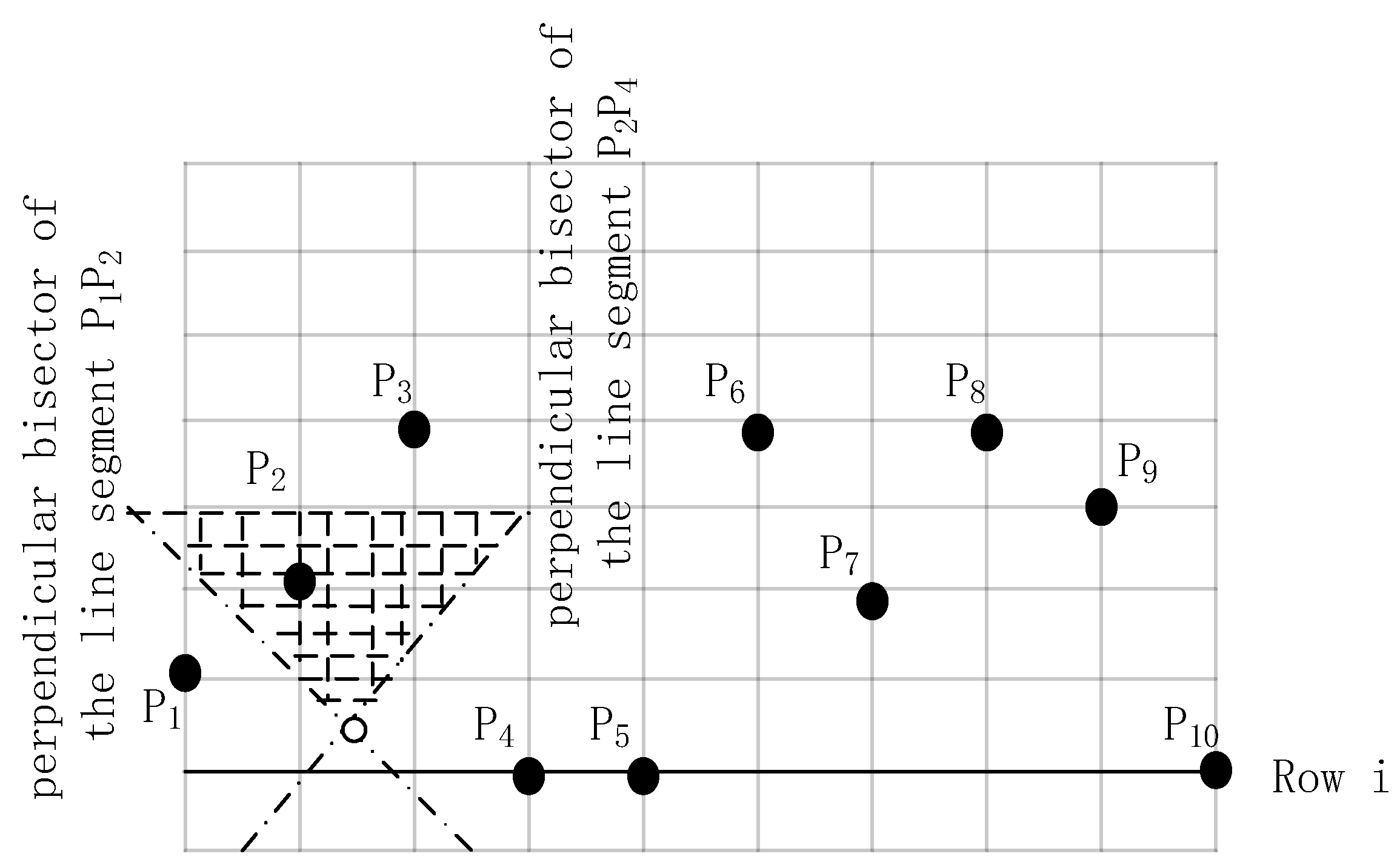
Figure 4 illustrates the concept of proximate-point masking. We consider only background pixels $P_1$, $P_2$ and $P_4$, which are also the proximate points of row $i-1$. The Voronoi cells associated with $P_1$ and $P_4$ intersect row i, making them valid proximate points for that row. The two dotted lines represent the perpendicular bisectors of the line segments $P_1{P}_2$ and $P_2{P}_4$. The intersection of these bisectors lies above row i, indicating that the Voronoi cell corresponding to $P_2$ (as dipicted by the background pattern in the figure) does not intersect this row. Because $P_2$ is dominated by $P_1$ and $P_4$, it is excluded from the proximate-point set of row i. Even when other proximate points in the figure are taken into account, the Voronoi cell corresponding to $P_2$ further shrinks and still does not intersect row i.

3.3.1. Computation of the Upper Proximate-Points Set for the First Row of Each Sub-Block

To compute the upper proximate-point set for the first row of each sub-block, the upper candidate proximate-point set obtained in Section 3.2 is used as input, and all geometrically dominated points are removed. The procedure operates as follows: each candidate proximate point is examined sequentially and inserted into the upper proximate-point set (e.g., points $P_1$–$P_{10}$ in Figure 4). After inserting a proximate point, the algorithm checks whether it masks one or more previously inserted proximate points. If masking occurs, the dominated points are removed from the upper proximate-point set. For example, when inserting $P_4$, the algorithm checks whether it masks $P_3$ or even $P_2$. The construction of the upper proximate-point set for the first row of each sub-block can be performed in parallel. The complete procedure is presented in Algorithm 1.

Algorithm 1 Computation of Upper Proximate-Points Sets of the First Row of Each Sub-block

Input: Upper candidate proximate-point matrix M;             Sub-blocks $S_1$, $S_2$, …, $S_k$. Output: Upper proximate-point sets of the first row of all sub-blocks: $Q_{1,1}$, $Q_{2,1}$, …, $Q_{k,1}$.  1: for all $i=1$ to k in parallel do  2:       Initialize an empty upper proximate-point set $Q_{i,1}$  3:       Retrieve the upper candidate proximate-point list $M_i$ from M  4:       for $j=1$ to $|M_i|$ do  5:            Extract the j-th candidate proximate point $P_j$ from $M_i$  6:            Insert $P_j$ into $Q_{i,1}$  7:            Check whether $P_j$ geometrically dominates one or more previously inserted proximate points  8:            if dominated points exist then  9:                 Remove all dominated proximate points from $Q_{i,1}$ 10:            end if 11:       end for 12: end for

The implementation details of the dominance test used in Line 7 of Algorithm 1 are provided in [27]. The procedure for computing the lower proximate-point set of the last row in each sub-block follows the same methodology and is therefore omitted for brevity.

3.3.2. Recurrence of the Upper Proximate-Point Set for the Next Row

Once the upper proximate-point set for a given row within a sub-block has been constructed, only a subset of these points remains valid for the subsequent row. The surviving points persist because they are not geometrically dominated by other proximate points, whereas dominated points are removed. In addition, the upper proximate-point set for row $i+1$ must incorporate all background pixels located on that row. Consequently, the key idea for deriving the upper proximate-point set of row $i+1$ is to identify which proximate points from row i become invalid due to geometric domination and then merge the remaining valid proximate points with the background pixels of the next row.

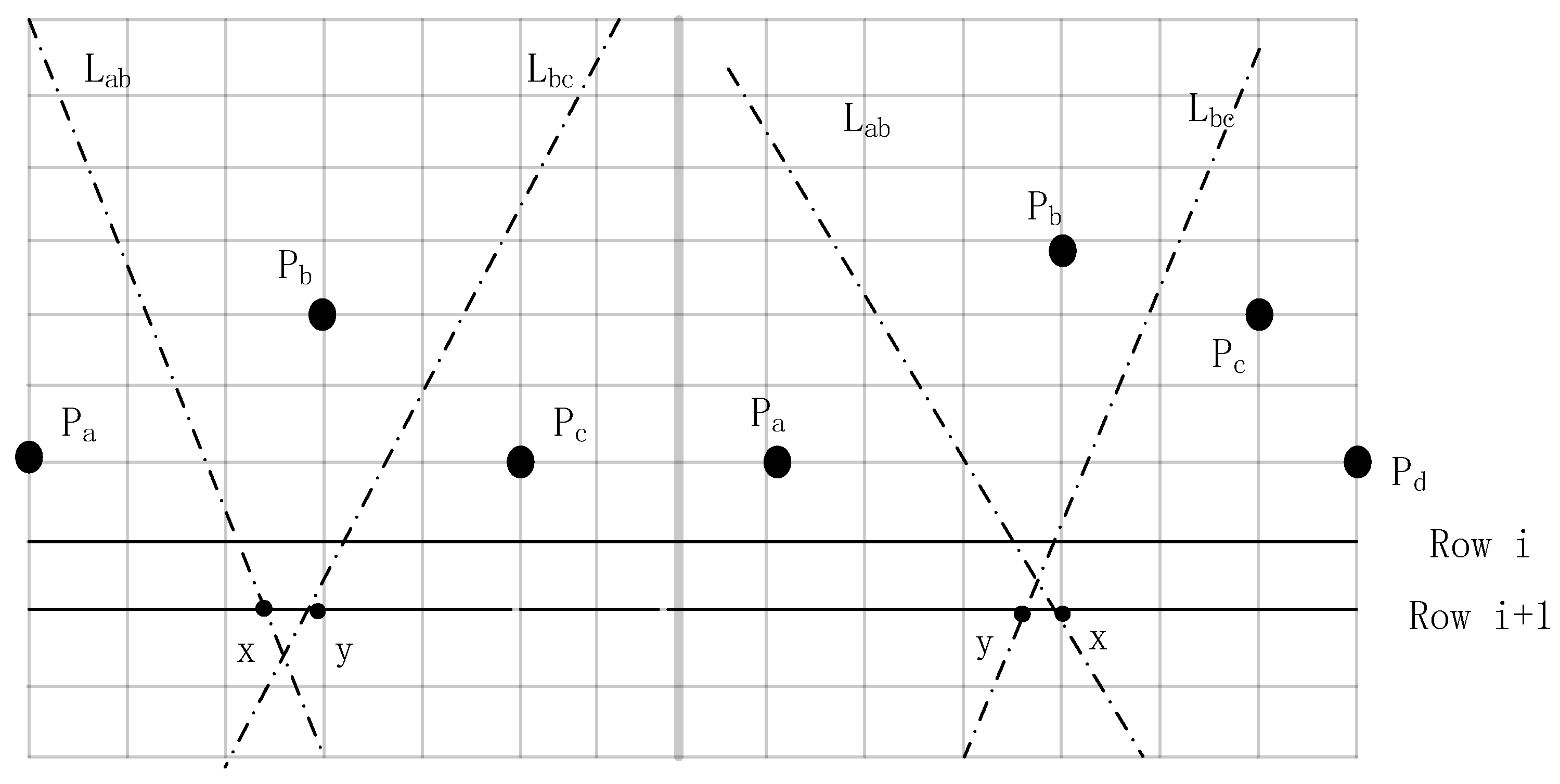
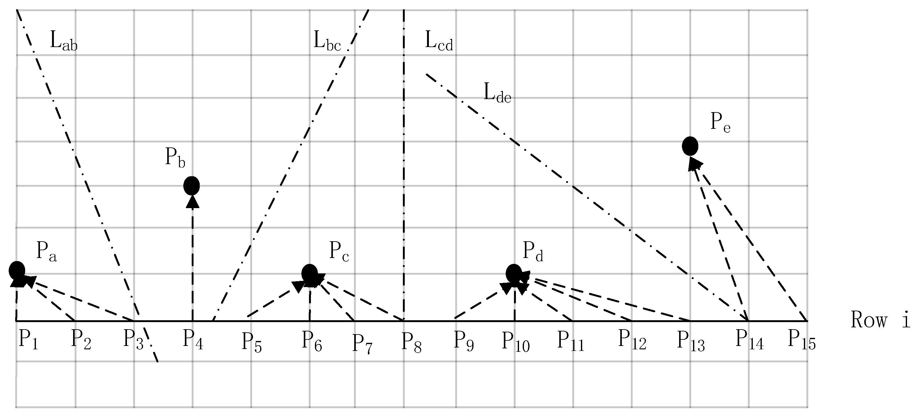
To determine whether a proximate point in row i remains valid in row $i+1$, every three consecutive proximate points ($P_a$, $P_b$, $P_c$) are grouped into a triplet, and the visibility of the middle point $P_b$ is evaluated. As illustrated in Figure 5, this evaluation examines whether $P_b$ is geometrically dominated by $P_a$ and $P_c$. Specifically, we compute the intersection points x and y between row $i+1$ and the perpendicular bisectors $L_{ab}$ and $L_{bc}$ of the point pairs ($P_a$, $P_b$) and ($P_b$, $P_c$), respectively.

If $x<y$, then point $P_b$ is the nearest background pixel to all positions in the interval $[x,y]$ on row $i+1$, and therefore remains in the upper proximate-point set of row $i+1$. Conversely, if $x>y$, the interval in which $P_b$ could be the closest background pixel collapses, indicating that $P_b$ is fully dominated; consequently, it is removed from the upper proximate-point set of row $i+1$.

As shown in Figure 5, the left-hand example illustrates a case in which $P_b$ remains valid in row $i+1$, while the right-hand example demonstrates a situation where $P_b$ becomes geometrically dominated by $P_a$ and $P_c$.

However, the above triplet-based method cannot identify all dominated proximate points in a single pass when multiple consecutive dominated points exist. For instance, in the right-hand case of Figure 5, both $P_b$ and $P_c$ are dominated. Yet, using the triplet 〈$P_b$, $P_c$, $P_d$〉 alone, it is not possible to determine whether $P_c$ is dominated by $P_b$ and $P_d$. Instead, multiple iterations of the triplet-checking procedure are required to fully detect all dominated points. Specifically, in the first iteration, the triplet 〈$P_a$, $P_b$, $P_c$〉 reveals that $P_b$ is dominated and should be removed. Only after removing $P_b$ can a second iteration detect that $P_c$ is also dominated, based on the updated triplet $\langle P_a,P_c,P_d\rangle$. More generally, if there are up to n consecutive dominated proximate points in the upper proximate-point set, the triplet-based evaluation must be executed up to n times to eliminate all dominated points.

To address this inefficiency, we introduce an enhanced strategy. After the initial triplet-based evaluation, dominated proximate points are removed immediately, and additional localized checks are performed around the removal positions to extend the detection range. Specifically, once a dominated proximate point (e.g., $P_b$) is eliminated, its adjacent neighbors (such as $P_a$ and $P_c$ in Figure 5) are immediately re-evaluated to determine whether they are also dominated. As stated in Algorithm 2, $P_c$ and the proximate points to its right are subsequently examined for dominance. This localized propagation mechanism substantially reduces the number of required passes, thereby improving the efficiency of dominated-point detection.

Algorithm 2 Detection of Consecutively Dominated Proximate Points

Input: Two proximate points $P_a$ and $P_c$; a sequence of proximate points $\{P_1,\dots ,P_k\}$ Output: A set of dominated proximate points   1: Begin   2: for $i=1$ to k do   3:       $P_t\leftarrow P_i$   4:       if $\mathrm{intersection}(P_a,P_c)\ge \mathrm{intersection}(P_c,P_t)$ then   5:            Mark $P_c$ as dominated   6:            $P_c\leftarrow P_t$   7:       else   8:            break   9:       end if 10: end for

After all dominated proximate points have been removed from the upper proximate-point set of row i, the background pixels of row $i+1$ are merged into the set to form the final upper proximate-point set for that row. During this merging process, each background pixel in row $i+1$ is inserted into the set according to its horizontal coordinate, and potential dominance relationships are re-evaluated. In particular, a newly inserted background pixel may dominate existing proximate points on either side; if so, the corresponding dominated proximate points are removed accordingly.

By repeating the above procedure, the upper proximate-point set can be computed for every row within each sub-block, as summarized in Algorithm 3. A symmetric procedure is applied to compute the lower proximate-point sets for all rows.

Algorithm 3 Computation of the Upper Proximate-Point Set for Row $i+1$

Input: Upper proximate-point sets of row i for all sub-blocks: $Q_{1,i},\dots ,Q_{k,i}$;             Background-pixel sets of row $i+1$ for all sub-blocks: $B_{1,i+1},\dots ,B_{k,i+1}$. Output: Upper proximate-point sets of row $i+1$ for all sub-blocks: $Q_{1,i+1}$, …, $Q_{k,i+1}$.  1: Begin  2: for all $r=1\dots k$ in parallel do  3:       Initialize $Q_{r,i+1}\leftarrow Q_{r,i}$  4:        $num\leftarrow |Q_{r,i}|$  5:      for all $j=2\dots num-1$ do  6:            Evaluate whether $P_j$ is dominated by $P_{j-1}$ and $P_{j+1}$  7:            if $P_j$ is dominated then  8:                Mark $P_j$ as dominated  9:            end if 10:           Check for consecutively dominated proximate points on the left of $P_j$ 11:           Check for consecutively dominated proximate points on the right of $P_j$ 12:      end for 13:      Compact $Q_{r,i+1}$ by removing all points marked as dominated 14:      Insert all background pixels in $B_{r,i+1}$ into $Q_{r,i+1}$ (ordered by x-coordinate) 15:      For each inserted background pixel, test and mark any proximate points it dominates (left/right) 16:      Compact $Q_{r,i+1}$ again to remove newly marked points 17: end for 18: End

During the execution of Algorithm 3, the proximate-point set of each sub-block is stored in the GPU’s shared memory, with each proximate point retaining its spatial coordinates. To enable parallel execution, each proximate point is assigned a dedicated thread. Once dominated proximate points are identified, they are marked for removal, and a parallel array-compaction procedure based on the prefix-sum algorithm [33] is applied to efficiently eliminate all marked elements from the set.

After compaction, the background pixels of the current image row are inserted into the remaining proximate-point set. For each inserted background pixel, dominance checks are performed on its immediate left and right neighbors to detect any newly dominated proximate points. These dominated points are subsequently marked and removed through a second array-compaction step. Through this iterative process, the proximate-point set is efficiently updated for each row while preserving both correctness and high parallel efficiency.

3.4. Euclidean Distance Computation

For each image row, a one-dimensional Voronoi diagram is constructed based on the upper proximate-point set. Each foreground pixel on that row identifies its nearest background pixel by determining the Voronoi cell to which it belongs and computing the corresponding Euclidean distance. Similarly, another one-dimensional Voronoi diagram is constructed using the lower proximate-point set, enabling each foreground pixel to obtain an additional candidate background pixel and its associated distance. Consequently, each foreground pixel produces two candidate distances, potentially corresponding to different background pixels, and the smaller of the two is selected as the final Euclidean distance to the nearest background pixel. Since the distance computations for all foreground pixels are mutually independent, they can be executed fully in parallel on the GPU, thereby substantially improving overall computational efficiency. Collectively, these distances form the final Euclidean distance map.

Figure 6 illustrates the construction of a one-dimensional Voronoi diagram on row i based on its upper proximate-point set. In this example, the row’s upper proximate-point set consists of five proximate points, denoted as $P_a$ through $P_e$. The perpendicular bisectors between adjacent proximate points partition the row into five Voronoi cells. The fifteen foreground pixels ($P_1$–$P_{15}$) on the row are assigned to the cell associated with the proximate point that yields the minimum Euclidean distance.

3.5. GPU Memory Organization and Thread Configuration

During execution, the input image, candidate proximate-point matrices, and intermediate proximate-point arrays are stored in global memory. Shared memory is employed within each thread block to cache proximate-point sets, thereby reducing global memory access latency.

For constructing the candidate proximate-point matrices, each image row is processed by a dedicated thread block, where one thread is assigned to each pixel. To compute the proximate-point sets, each sub-block is handled by a single thread block, in which multiple threads collaboratively process individual rows in parallel. The number of concurrent threads is determined by the image width and the CUDA block configuration, ensuring sufficient parallelism while remaining within shared memory constraints.

Finally, for Euclidean distance computation, one thread block is assigned to each image row, enabling parallel distance evaluation for all foreground pixels in that row.

3.6. Time Complexity Analysis

Assume that the image has n rows and n columns and is partitioned into k sub-blocks. In Step 2, the algorithm performs two full-image scans to compute the upper and lower candidate proximate-point sets, resulting in a computational complexity of $O\left(n^2\right)$. With n processors executing the scan in parallel, the theoretical time complexity can be reduced to $O\left(n\right)$.

In Step 3, computing the upper or lower proximate-point set for an arbitrary image row from its candidate proximate-point sets requires $O\left(n\right)$ time. Hence, the total cost of computing the upper proximate-point sets of the first row and the lower proximate-point sets of the last row for all k sub-blocks is $O\left(kn\right)$. With k processors performing these tasks in parallel, the theoretical time complexity decreases to $O\left(n\right)$. For the remaining rows, the proximate-point sets can be computed using a recursive update strategy. Since each row requires processing $O\left(n\right)$ proximate points, the complexity for a single row is $O\left(n\right)$, and the total complexity for all n rows in all k sub-blocks is $O\left(n^2\right)$. According to the parallel strategy adopted in Algorithm 3, this stage can theoretically be executed using $O\left(kn\right)$ parallel processors, reducing the time complexity to $O(n/k)$.

In Step 4, constructing the Voronoi diagram for each row based on its $O\left(n\right)$ proximate points incurs $O\left(n^2\right)$ computational cost. Additionally, computing the Euclidean distance from each foreground pixel to its nearest background pixel also requires $O\left(n^2\right)$ operations. If $O\left(n^2\right)$ processors were available to carry out all these tasks in parallel, the time complexity of this stage could be reduced to $O\left(1\right)$.

In summary, the theoretical time complexity of the proposed parallel Euclidean distance transform algorithm is $O\left(n\right)$. However, as noted in [23], a noticeable gap often exists between the theoretical complexity of Euclidean distance transform algorithms and their actual performance on GPU platforms. Many algorithms that exhibit favorable theoretical complexity fail to achieve the expected efficiency in practical GPU execution. A primary reason for this discrepancy is that theoretical analyses often rely on idealized assumptions, such as the availability of an unlimited number of processing units. In real systems, however, hardware resources are inherently constrained. For example, in Step 3, achieving the theoretical time complexity of $O(n/k)$ requires the GPU to provide $O\left(kn\right)$ concurrent threads to process the recursive updates of proximate-point sets for all rows. In practice, the maximum number of concurrently active threads is limited by the GPU architecture, making such large-scale parallelism unattainable.

Another major factor that impacts GPU performance is the memory access pattern. In [24,25,26], the algorithms perform frequent insertions and deletions on the proximate-point sets of each row, which are stored using non-contiguous data structures such as linked lists. These structures prevent efficient utilization of memory coalescing—a key feature for achieving high memory throughput on GPUs. As a result, memory access efficiency is significantly reduced, which in turn limits the overall performance.

4. Experiments and Results Analysis

4.1. Experimental Setup

The experiments in this paper were conducted on an NVIDIA A10 GPU platform equipped with 28 streaming multiprocessors (SMs), a 4 MB L2 cache, and 164 KB of shared memory. All GPU implementations were compiled and executed using the CUDA Toolkit 10.1. The serial algorithms were benchmarked on an Intel Xeon Gold 5320 processor.

For clarity in presenting the experimental results, the parallel EDT algorithm proposed by Duhu Man in [24,25] is referred to as the Man algorithm, the parallel EDT algorithm proposed by Dale Black in [29] is referred to as the Black algorithm, whereas the method proposed in this paper is referred to as the Partition-Based Recursive EDT (PR-EDT) algorithm.

To facilitate performance evaluation, three speedup metrics are introduced. The first metric, $S_1$, is defined as the ratio of the execution time of the serial EDT algorithm to that of the Man algorithm:

$$S_1={\displaystyle \frac{T_{serial}}{T_{Man}}}$$

(1)

Similarly, the second metric, $S_2$, is defined as the ratio of the serial EDT execution time to that of the Black algorithm, i.e.,

$$S_2={\displaystyle \frac{T_{serial}}{T_{Black}}}$$

(2)

Similarly, the third metric, $S_3$, is defined as the ratio of the serial EDT execution time to that of the PR-EDT algorithm, i.e.,

$$S_3={\displaystyle \frac{T_{serial}}{T_{PR}}}$$

(3)

Here, $T_{\mathrm{serial}}$ denotes the execution time of the serial algorithm, $T_{\mathrm{Man}}$ represents the execution time of the Man algorithm, $T_{\mathrm{Black}}$ represents the execution time of the Black algorithm, and $T_{\mathrm{PR}}$ corresponds to the execution time of the PR-EDT algorithm.

The objectives of our experiments are five-fold:

• to evaluate the performance overhead and time distribution of each step in the PR-EDT algorithm;
• to compare the performance of the PR-EDT algorithm with that of the optimized serial algorithm [27], the Man algorithm [24,25] and the Black algorithm [29];
• to examine the adaptability and efficiency of the algorithm when applied to images with varying levels of background-pixel sparsity; and
• to assess the impact of the sub-block size on the overall performance.
• to compare the memory usage of the PR-EDT algorithm with that of the optimized serial algorithm, the Man algorithm and the Black algorithm.

We use four categories of image samples with different resolutions (1024 × 1024, 2048 × 2048, 4096 × 4096, and 8192 × 8192). The proportion of background pixels is adjusted according to the experimental requirements.

To ensure experimental reproducibility, all test images are randomly generated using a fixed random seed (seed = 42). For each image resolution and background-pixel density, the same seed is consistently applied across all runs, guaranteeing identical input data for all compared methods. Each experiment is repeated 20 times on the same generated image, and the reported execution time is the average over these runs. In addition, the results produced by the PR-EDT algorithm are compared against those of the serial algorithm on a pixel-by-pixel basis to verify the correctness of the proposed method.

In the experiments presented in Section 4.2, Section 4.3 and Section 4.4, the number of rows in each sub-block is fixed at 20.

4.2. Performance Analysis of Each Step in the PR-EDT Algorithm

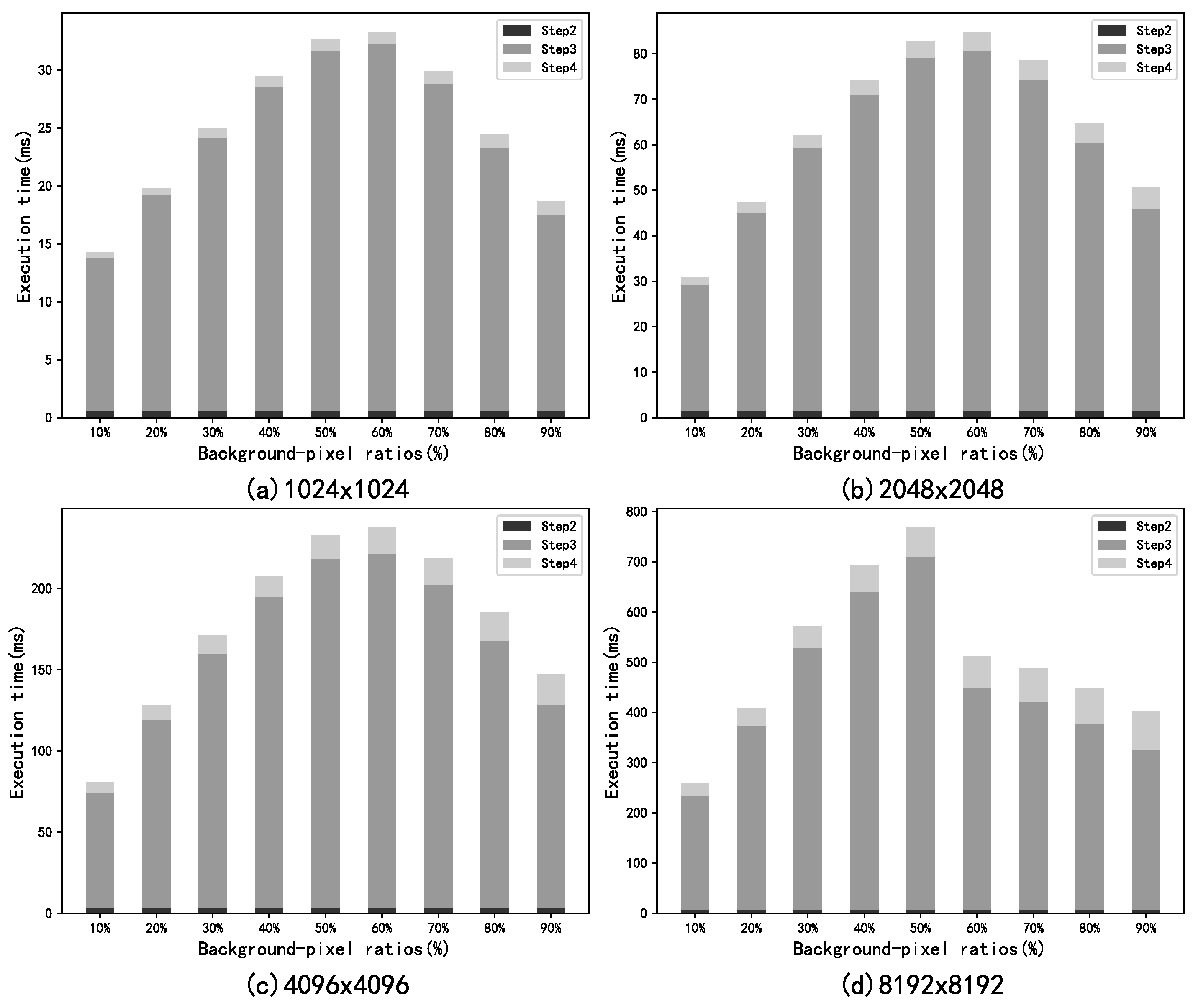
To analyze the behavior of the PR-EDT algorithm under different image characteristics, we conducted experiments on images with background-pixel ratios ranging from 10% to 90%. We measured the execution time of Step 2, Step 3, and Step 4, while Step 1 was omitted because its overhead is negligible. On average, Step 2, Step 3, and Step 4 accounted for approximately 1.69%, 88.59%, and 9.72% of the total runtime, respectively. The time distribution of these three steps under varying image conditions is shown in Figure 7.

Step 3 computes the upper and lower proximate-point sets for each row within every sub-block. As the proportion of background pixels increases, the number of candidate proximate points also increases. For example, in an 8192 × 8192 image, the candidate proximate-points set contains 2623 points when the background-pixel ratio is 1%, but the number increases to 7187 when the ratio reaches 57%. Consequently, for images of the same resolution, Step 3 generally generally requires more execution time as the background-pixel ratio increases.

The execution time of Step 3 peaks when the background-pixels ratio is around 57%. Interestingly, when the ratio increases beyond this point, the execution time begins to decrease. This behavior occurs because higher background-pixel density increases the likelihood that candidate proximate points form long consecutive segments within a row. The PR-EDT algorithm is particularly efficient at handling such consecutively distributed candidate points, for example by quickly eliminating long runs of dominated proximate points. As a result, despite the larger candidate proximate-point set, the overall computational cost of Step 3 decreases when background pixels become highly dense.

4.3. Performance Comparison with the Serial, Man, and Black Algorithms

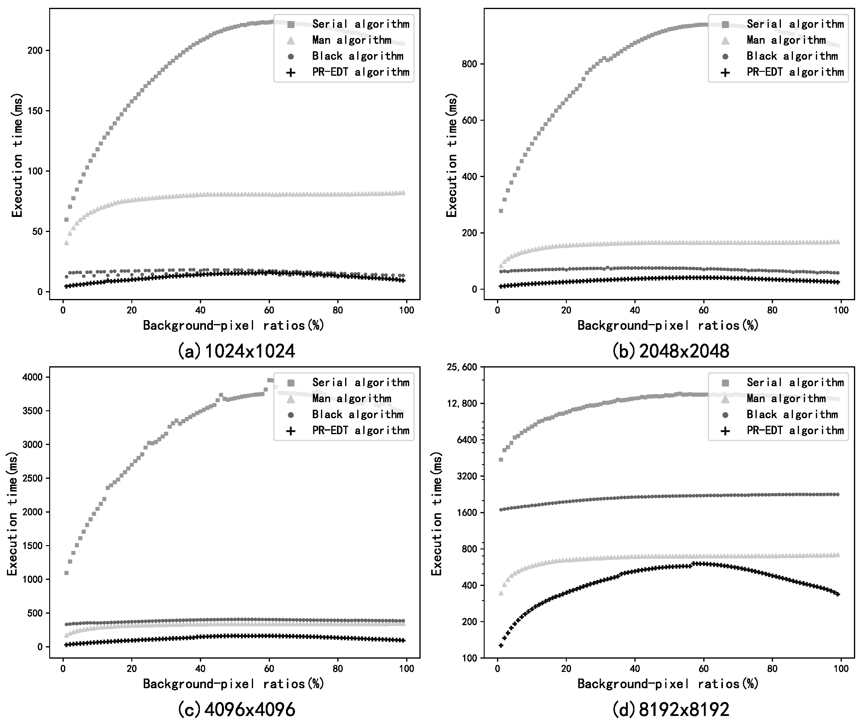
To comprehensively evaluate the performance of the serial algorithm, the Man algorithm, and the PR-EDT algorithm, we conducted experiments on images with four different resolutions and varying background-pixel ratios. The experimental results are summarized in Figure 8. As the image resolution increases, the performance advantage of the PR-EDT algorithm becomes increasingly pronounced, consistently outperforming the serial, Man, and Black algorithms.

4.4. Performance Comparison of the Algorithm on Images with Sparse and Dense Background Pixels

To evaluate the impact of background-pixel density on algorithmic performance, we conducted experiments on four image resolutions using the serial algorithm, the Man algorithm, the Black algorithm, and the proposed PR-EDT algorithm. For each resolution, two image types were generated: one with a background-pixel ratio of 1% and another with 99%, corresponding to sparse and dense background-pixel distributions, respectively. These test cases enable a comprehensive assessment of the adaptability and efficiency of the three algorithms under varying background-pixel conditions.

Table 1. Execution time comparison of the serial algorithm, the Man algorithm, the Black algorithm, and the PR-EDT algorithm under different image resolutions and background-pixel ratios.

Image Resolution/Background Ratio	Serial (ms)	Man (ms)	Black (ms)	PR-EDT (ms)	${\mathit{S}}_1$	${\mathit{S}}_2$	${\mathit{S}}_3$
1024 × 1024 (1%)	59.77	40.58	12.40	7.68	1.47	4.82	7.78
2048 × 2048 (1%)	278.37	82.88	62.52	13.3	3.35	4.45	20.93
4096 × 4096 (1%)	1094.07	169.22	333.11	28.08	6.46	3.28	38.96
8192 × 8192 (1%)	4380.63	344.24	1688.41	84.19	12.72	2.59	52.03
1024 × 1024 (99%)	205.39	82.05	13.45	14.15	2.50	15.27	14.51
2048 × 2048 (99%)	864.44	168.04	58.09	39.24	5.14	14.88	22.02
4096 × 4096 (99%)	3484.25	343.88	385.77	116.77	10.13	9.03	29.83
8192 × 8192 (99%)	13,862.27	713.49	2256.60	341.91	19.42	6.14	40.54

summarizes the execution times of the algorithms (in milliseconds) and reports the speedup of the Man algorithm over the serial baseline (S1), the speedup of the Black algorithm over the serial baseline (S2), as well as the speedup of the PR-EDT algorithm over the serial baseline (S3).

The results in Table 1 show that the PR-EDT algorithm consistently outperforms the serial, Man and Black algorithms across all resolutions and background-pixel ratios. For any fixed resolution, the PR-EDT algorithm achieves greater speedup on background-dense images. This behavior arises because the serial algorithm processes each background pixel independently, regardless of its distribution, whereas the PR-EDT algorithm efficiently handles groups of consecutively distributed background pixels (proximate points), leading to more substantial acceleration in dense-background scenarios. Although the Man and Black algorithm yields noticeable improvement over the serial algorithm, its performance remains significantly inferior to that of the PR-EDT algorithm under both sparse and dense background-pixel distributions.

4.5. Performance Analysis Under Varying Sub-Block Sizes

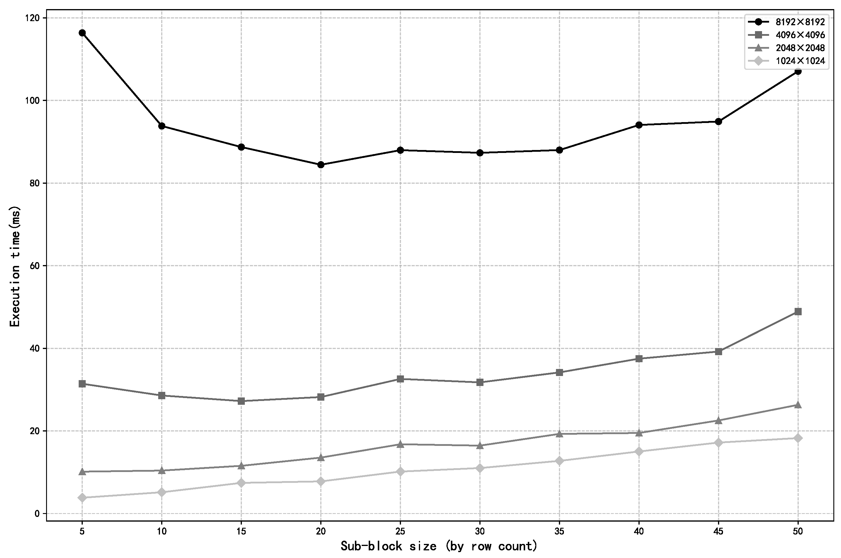
To evaluate the impact of sub-block size on the performance of the PR-EDT algorithm, experiments were conducted on images with resolutions of 1024 × 1024, 2048 × 2048, 4096 × 4096, and 8192 × 8192, while fixing the background-pixel ratio at 1%. The algorithm was tested with multiple sub-block configurations, and the results are shown in Figure 9.

Selecting an appropriate sub-block size requires balancing two competing factors. On the one hand, proximate-point recursion is performed within each sub-block; thus, increasing the number of rows per sub-block reduces the local computational overhead. On the other hand, larger sub-blocks yield fewer total sub-blocks, which in turn decreases the degree of global parallelism. As shown in Figure 9, configuring each sub-block to contain approximately 20 rows provides consistently optimal performance across all tested image resolutions.

4.6. Memory Usage Analysis

Table 2. Memory usage comparison of the serial algorithm, the Man algorithm, the Black algorithm, and the PR-EDT algorithm under different image resolutions.

Image Resolution	Serial (MiB)	Man (MiB)	Black (MiB)	PR-EDT (MiB)
1024 × 1024	17	624	34	258
2048 × 2048	68	748	84	324
4096 × 4096	272	1240	275	588
8192 × 8192	1088	3210	1090	1644

compares the memory usage of the serial algorithm, the Man algorithm, the Black algorithm, and the proposed PR-EDT algorithm under different image resolutions.

As expected, the memory consumption of all algorithms increases with image resolution. The serial algorithm exhibits the lowest memory usage, since it only stores the input image and intermediate distance maps. The Man algorithm requires significantly more memory due to the storage of multiple auxiliary arrays and intermediate data structures during parallel computation.

Compared with the Man algorithm, the PR-EDT algorithm substantially reduces memory usage by partitioning the image into sub-blocks and processing them independently, thereby limiting the size of auxiliary data structures. Although the PR-EDT algorithm consumes more memory than the serial and Black algorithms, it achieves a favorable trade-off between memory usage and computational efficiency. The additional memory overhead of PR-EDT mainly comes from storing candidate proximate-point matrices and sub-block-level auxiliary data, which are essential for enabling efficient parallel processing and reducing redundant distance computations.

5. Limitations and Scalability Analysis

Despite the significant performance improvement achieved by the PR-EDT algorithm, several limitations should be acknowledged to provide a comprehensive and balanced evaluation of the method.

5.1. GPU Memory Constraints

The PR-EDT algorithm relies on storing the input image, the background-pixels for each image row, candidate proximate-point matrix, proximate points for each image row and auxiliary buffers in GPU global memory. While this design enables high parallel efficiency, it inherently limits the maximum image resolution that can be processed on a single GPU. For extremely large-scale images, the memory consumption of intermediate data structures may exceed the available GPU memory capacity, thereby restricting scalability in single-GPU environments.

In the current implementation, all sub-blocks are processed in-core to minimize data transfer overhead between host and device memory. As a result, the method is most suitable for scenarios where the entire dataset can reside in GPU memory. Extending the algorithm to support out-of-core processing or memory streaming would be necessary to handle ultra-high-resolution images.

5.2. Scalability with Image Resolution and Sub-Block Partitioning

Although the computational complexity of the PR-EDT algorithm scales favorably with image size, practical scalability is influenced by several GPU-specific factors. The horizontal sub-block partitioning strategy introduces a trade-off between parallelism and overhead. Smaller sub-blocks increase the degree of parallel execution but may incur more redundant computation, whereas larger sub-blocks reduce overall computation but limit concurrency.

Furthermore, as image resolution increases, the algorithm becomes increasingly sensitive to memory bandwidth saturation and cache utilization efficiency. While the row-wise recursive construction of Voronoi diagrams effectively reduces redundant computation, the overall performance may eventually be bounded by memory access patterns rather than arithmetic intensity.

6. Conclusions

For the two-dimensional exact Euclidean distance transform (EDT) problem, this work proposes a row-wise recursive parallel algorithm, termed PR-EDT, which is constructed upon the classical Voronoi-intersection approach. By fully exploiting the structural similarity between the Voronoi diagrams of adjacent rows, the PR-EDT algorithm efficiently builds the Voronoi diagram within each sub-block, thereby reducing computational complexity and significantly improving overall performance. Experimental evaluations show that the PR-EDT algorithm achieves up to a 52× speedup on GPU platforms compared with traditional CPU-based methods. The core idea of exploiting inter-row structural similarity during Voronoi diagram construction is, in principle, extendable to higher-dimensional exact and approximate EDT formulations, as the underlying algorithmic structure is dimension-independent. However, such extensions would significantly increase memory requirements and data dependency complexity, posing additional challenges for efficient GPU implementation. Moreover, the current work focuses on a single-GPU execution model. Scaling the proposed approach to multi-GPU systems would require careful redesign of data partitioning and inter-device communication mechanisms to maintain consistency across sub-block boundaries. Investigating efficient multi-GPU and distributed implementations is therefore identified as an important direction for future research.

References

1. Fabbri, R.; Costa, L.d.F.; Torelli, J.C.; Bruno, O.M. 2D Euclidean distance transform algorithms: A comparative survey. ACM Comput. Surv. 2008, 40, 1–44. [Google Scholar] [CrossRef]
2. Mussabayev, R. Optimizing Euclidean Distance Computation. Mathematics 2024, 12, 3787. [Google Scholar] [CrossRef]
3. Cuisenaire, O.; Macq, B. Fast and exact signed Euclidean distance transformation with linear complexity. In Proceedings of the IEEE International Conference on Acoustics, Speech, and Signal Processing, Phoenix, AZ, USA, 15–19 March 1999; pp. 3293–3296. [Google Scholar] [CrossRef]
4. Shih, F.Y.; Wu, Y.T. Fast Euclidean distance transformation in two scans using a 3 × 3 neighborhood. Comput. Vis. Image Underst. 2004, 93, 195–205. [Google Scholar] [CrossRef]
5. Shih, F.Y.; Wu, Y.T. The efficient algorithms for achieving Euclidean distance transformation. IEEE Trans. Image Process. 2004, 13, 1078–1091. [Google Scholar] [CrossRef] [PubMed]
6. Cuisenaire, O.; Macq, B. Fast Euclidean distance transformations by propagation using multiple neighborhoods. Comput. Vis. Image Underst. 1999, 76, 163–172. [Google Scholar] [CrossRef]
7. Eggers, H. Two fast Euclidean distance transformations in Z2 based on sufficient propagation. Comput. Vis. Image Underst. 1998, 69, 106–116. [Google Scholar] [CrossRef]
8. Paglieroni, D.W. Distance transforms: Properties and machine vision applications. CVGIP Graph. Model. Image Process. 1992, 54, 56–74. [Google Scholar] [CrossRef]
9. Paglieroni, D.W. A unified distance transform algorithm and architecture. Mach. Vis. Appl. 1992, 5, 47–55. [Google Scholar] [CrossRef]
10. Hirata, T. A unified linear-time algorithm for computing distance maps. Inf. Process. Lett. 1996, 58, 129–133. [Google Scholar] [CrossRef]
11. Lotufo, R.A.; Zampirolli, F.A. Fast multidimensional parallel Euclidean distance transform based on mathematical morphology. In Proceedings of the Brazilian Symposium on Computer Graphics and Image Processing, Florianopolis, Brazil, 15–18 October 2001; pp. 100–105. [Google Scholar] [CrossRef]
12. Maurer, C.R.; Raghavan, V.; Qi, R. A linear time algorithm for computing the Euclidean distance transform in arbitrary dimensions. In Proceedings of the Information Processing in Medical Imaging, Davis, CA, USA, 18–22 June 2001; pp. 358–364. [Google Scholar] [CrossRef]
13. Silva, D.J.; Miranda, P.A.V.; Alves, W.A.L.; Hashimoto, R.F.; Kosinka, J.; Roerdink, J.B.T.M. Differential maximum Euclidean distance transform computation in component trees. In Proceedings of the International Conference on Discrete Geometry and Mathematical Morphology, Florence, Italy, 15–18 April 2024; pp. 67–79. [Google Scholar] [CrossRef]
14. Ali, U.; Wu, L.; Müller, A.; Sukkar, F.; Kaupp, T.; Vidal-Calleja, T.A. Interactive Distance Field Mapping and Planning to Enable Human-Robot Collaboration. IEEE Robot. Autom. Lett. 2024, 9, 10850–10857. [Google Scholar] [CrossRef]
15. Elizondo-Leal, J.C.; Ramirez-Torres, J.G.; Barrón-Zambrano, J.H.; Diaz-Manríquez, A.; Nuño-Maganda, M.A.; Saldivar-Alonso, V.P. Parallel raster scan for Euclidean distance transform. Symmetry 2020, 12, 1808. [Google Scholar] [CrossRef]
16. Aaa, M.; Dorent, R.; Vercauteren, T. FastGeodis: Fast generalised geodesic distance transform. J. Open Source Softw. 2022, 7, 4532. [Google Scholar] [CrossRef]
17. Criminisi, A.; Sharp, T.; Siddiqui, K. Interactive geodesic segmentation of n-dimensional medical images on the graphics processor. In Proceedings of the Radiological Society of North America, Chicago, IL, USA, 29 November–4 December 2009. [Google Scholar]
18. He, X.; Agarwal, D.; Prasad, S.K. Design and implementation of a parallel priority queue on many-core architectures. In Proceedings of the International Conference on High Performance Computing, Pune, India, 18–22 December 2012; pp. 1–10. [Google Scholar] [CrossRef]
19. He, X.; Wu, Y.; Di, Z.; Chen, J. GPU-based morphological reconstruction system. J. Comput. Appl. 2019, 39, 2008–2013. [Google Scholar] [CrossRef]
20. Rong, G.; Tan, T.S. Variants of jump flooding algorithm for computing discrete Voronoi diagrams. In Proceedings of the International Symposium on Voronoi Diagrams in Science and Engineering, Glamorgan, UK, 9–11 July 2007; pp. 176–181. [Google Scholar] [CrossRef]
21. Cuntz, N.; Kolb, A. Fast Hierarchical 3D Distance Transforms on the GPU; The Eurographics Association: Eindhoven, The Netherlands, 2007; pp. 93–96. [Google Scholar] [CrossRef]
22. Zampirolli, F.D.A.; Filipe, L. Distance transform separable by mathematical morphology in GPU. In Proceedings of the Progress in Pattern Recognition, Image Analysis, Computer Vision, and Applications, Havana, Cuba, 20–23 November 2013; pp. 41–48. [Google Scholar] [CrossRef]
23. Cao, T.T.; Tang, K.; Mohamed, A.A.; Tan, T.S. Parallel banding algorithm to compute exact distance transform with the GPU. In Proceedings of the ACM on Computer Graphics and Interactive Techniques, Los Angeles, CA, USA, 26–30 July 2010; pp. 83–90. [Google Scholar] [CrossRef]
24. Man, D.; Uda, K.; Ueyama, H.; Ito, Y.; Nakano, K. Implementations of parallel computation of Euclidean distance map in multicore processors and GPUs. In Proceedings of the International Conference on Networking & Computing, Washington, DC, USA, 30 November–2 December 2011; pp. 120–127. [Google Scholar] [CrossRef]
25. Man, D.; Uda, K.; Ito, Y.; Nakano, K. Accelerating computation of Euclidean distance map using the GPU with efficient memory access. Int. J. Parallel Emergent Distrib. Syst. 2013, 28, 383–406. [Google Scholar] [CrossRef]
26. Mandudu, M.; Jones, M.W. A work efficient parallel algorithm for exact Euclidean Distance Transform. IEEE Trans. Image Process. 2019, 28, 5322–5335. [Google Scholar] [CrossRef] [PubMed]
27. Breu, H.; Gil, J.; Kirkpatrick, D.; Werman, M. Linear time Euclidean distance transform algorithms. IEEE Trans. Pattern Anal. Mach. Intell. 2002, 17, 529–533. [Google Scholar] [CrossRef]
28. Chen, Y.; Lai, S.; Cui, J.; Wang, B.; Chen, B.M. GPU-accelerated incremental Euclidean distance transform for online motion planning of mobile robots. IEEE Robot. Autom. Lett. 2022, 7, 6894–6901. [Google Scholar] [CrossRef]
29. Black, D.; Li, W.; Zhang, Q.; Molloi, S. Accelerating Euclidean distance transforms: A fast and flexible approach with multi-vendor GPU, multi-threading, and multi-language support. IEEE Access 2025, 13, 44636–44649. [Google Scholar] [CrossRef]
30. Gallet, B.; Michael, G. Leveraging GPU tensor cores for double precision Euclidean distance calculations. In Proceedings of the International Conference on High Performance Computing, Data, and Analytics (HiPC), Bengaluru, India, 18–21 December 2022; pp. 135–144. [Google Scholar] [CrossRef]
31. Zhu, D.; Wang, C.; Wang, W.; Garg, R.; Scherer, S.; Meng, M.Q.H. VDB-EDT: An Efficient Euclidean Distance Transform Algorithm Based on VDB Data Structure. arXiv 2021, arXiv:2105.04419. [Google Scholar] [CrossRef]
32. Han, X.; Zeng, P. A Hardware Design of EDT Algorithm Applied to Binary Images. In Proceedings of the International Conference on Computer Science and Electronics Engineering; IEEE: Piscataway, NJ, USA, 2013. [Google Scholar] [CrossRef][Green Version]
33. Sengupta, S.; Harris, M.; Zhang, Y.; Owens, J.D. Scan primitives for GPU computing. In Proceedings of the ACM Eurographics Workshop on Graphics Hardware, San Diego, CA, USA, 4–5 August 2007; pp. 97–106. [Google Scholar] [CrossRef]
Figure 1. Illustration of a 5 × 5 binary image in a two-dimensional coordinate system and its corresponding Voronoi diagram.
Mathematics 14 00597 g001
Figure 3. Compute the upper/lower candidate proximate-point matrices.
Mathematics 14 00597 g003
Figure 4. Illustration of proximate-point masking.
Mathematics 14 00597 g004
Figure 5. Determining whether a proximate point is dominated.
Mathematics 14 00597 g005
Figure 6. Construction of a one-dimensional Voronoi diagram based on the upper proximate-point set.
Mathematics 14 00597 g006
Figure 7. Performance Analysis of Each Step in the PR-EDT Algorithm.
Mathematics 14 00597 g007
Figure 8. Performance Analysis of Four Algorithms.
Mathematics 14 00597 g008
Figure 9. Performance Comparison under Varying Sub-Block Sizes.
Mathematics 14 00597 g009