A Well-Balanced Wet–Dry Front Reconstruction for Two-Layer Shallow Water Flows

Abstract
1. Introduction
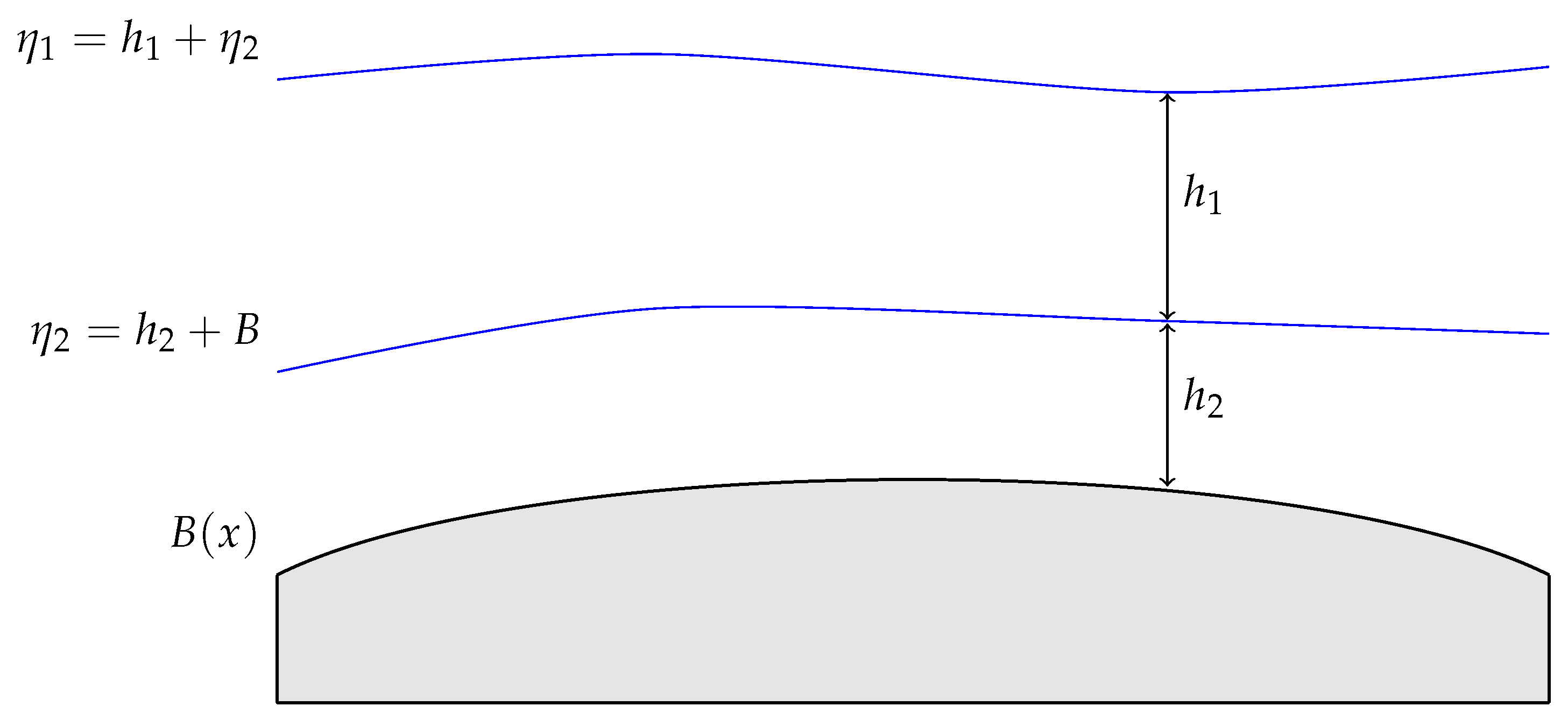
2. A Finite Volume Scheme for the Two-Layer Shallow Water Equations
3. A New Reconstruction for Two-Layer SWEs with Wet–Dry Fronts
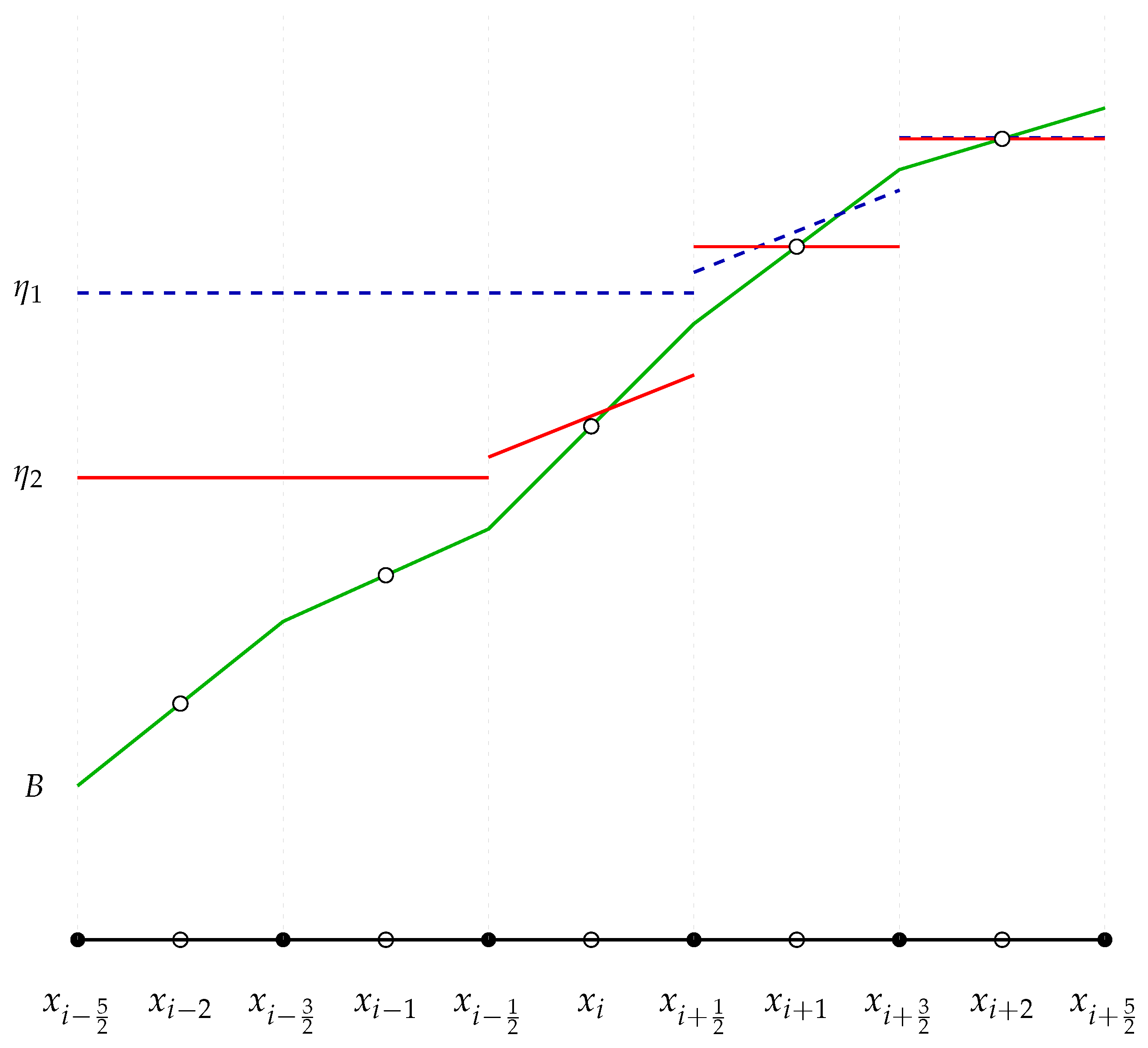
3.1. Piecewise Linear Reconstruction for Flux Variables
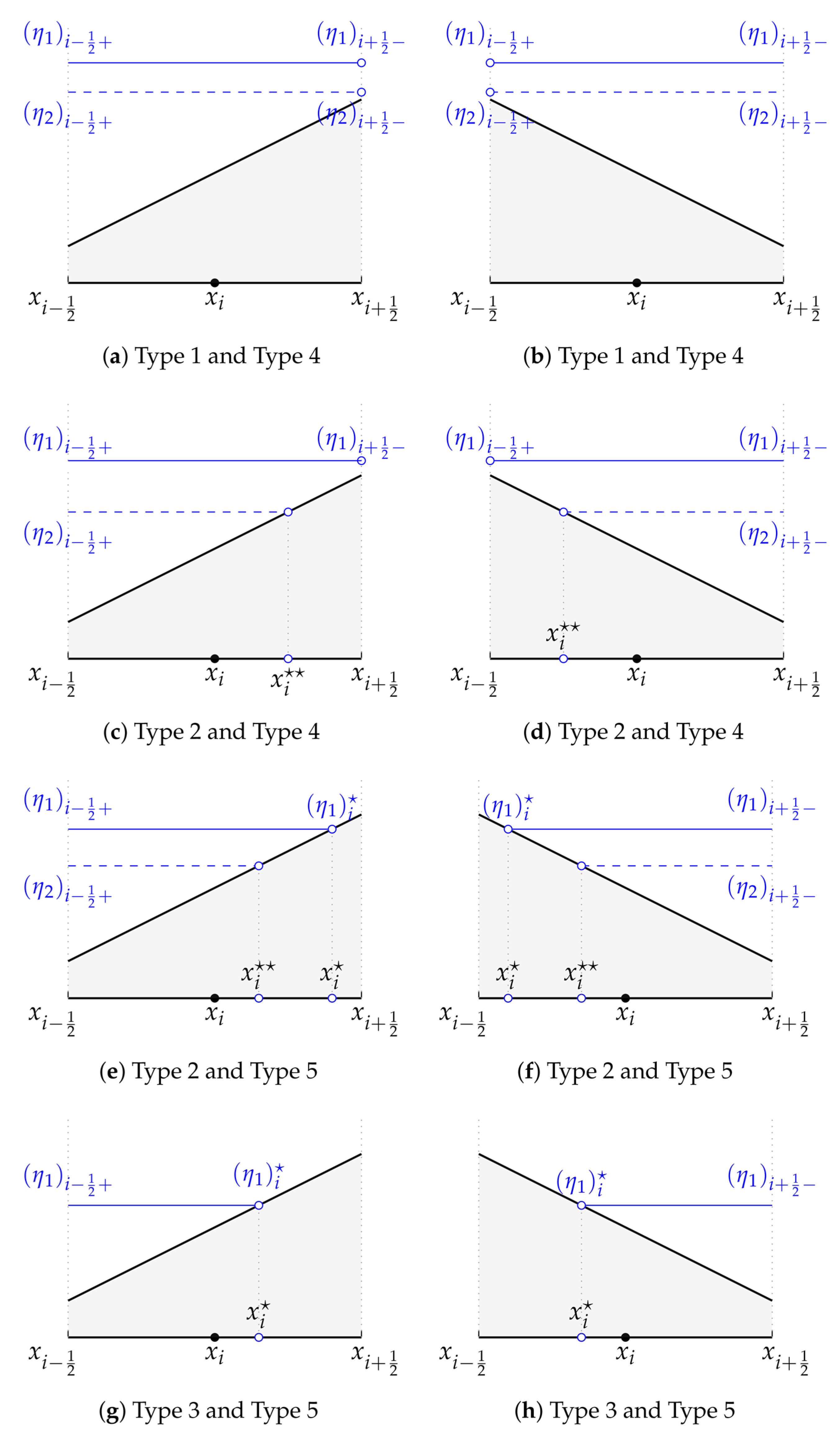
3.2. Correction of Surface Reconstruction for Two-Layer Fluid Systems
- Type 1: Fully flooded cell: ,
- Type 2: Partially flooded cell: ,
- Type 3: Dry cell: ,
- Type 4: Fully flooded cell: ,
- Type 5: Partially flooded cell: ,
- Type 6: Dry cell: ,
- Step 1: Reconstruct the lower layer fluid using the method from [27]:
- In the lower fluid layer, the cell is a fully flooded cell , i.e., it belongs to Type 1. The corrected water depth expression is as follows:whereso the layer interface is
- In the Type 2 cell , assuming that water is distributed in the lower region of the bottom while the higher region remains dry, without loss of generality, we consider an increasing bottom: . The expression for the layer interface is then given bywhere denotes the water depth at the wet vertex of the cell , represents the position of the wet–dry front, and is the length of the wet subregion within the cell. In the following, we will define and sequentially.
- (1)
- First, we define the value at the left edge of the cell , with the specific form given bywhere denotes the steady free surface of the lower layer fluid, i.e., the water is at rest, expressed asThe extrapolated value is computed starting from the left neighboring cell under the condition that it is fully filled with water. Specifically, the expression for calculating is given by
- (2)
- Next, the wet–dry front is reconstructed. Using the conservation of water mass within this cell, we obtainthen the length of the wet sub-interval within the cell can be determined, thereby locating the position of the wet–dry front:The inequality indicates the presence of the wet–dry front within the cell.
Thus the wet–dry front reconstruction is completed, and a similar procedure is applied for the case where . - When the cell belongs to Type 3, i.e., in cell , we directly set
- Step 2: Correction of the surface reconstruction for the upper layer fluid.
- In the fully flooded cell , i.e., the cell belongs to Type 4, the water surface reconstruction for the lower layer has been completed. Denote and as the reconstructed water surface values of the lower layer at the two endpoints of the cell . Assuming the current water surface values of the upper layer at the two endpoints are and , two cases need to be discussed:
- (1)
- If and , the water surface requires no correction, we let
- (2)
- Otherwise, the reconstructed upper-layer water depth at the cell interface is negative; a case-by-case analysis is required.
- —
- If , ⟹
- —
- If , ⟹
The expression for the free surface is - In the partially flooded cell , i.e., the cell of Type 5, the water is assumed to occupy the lower part of the bottom, while the higher part remains dry. Without loss of generality, we consider the case where . The expression for the free surface is then given as follows:where , is the values defined in (28), denotes the position of the wet–dry front at the free surface, we will proceed to define and sequentially.
- (1)
- We first define as the free surface value at the cell edge ,where the extrapolated value is obtained using the endpoint value from the left neighbor cell under the fully flooded state; Specifically, the expression for is given byHere, represents the free surface level when the entire fluid is in the static steady state, given byNext, we determine the upper bound and lower bound for . According to the mass conservation of water, their expressions are given as follows:where and . We next proceed to determine the values of a and b. First, b is set as , where the value of is calculated as follows:where is the surface value of the lower layer fluid at the endpoint , defined by (28), the mass conservation law then gives .Next, we define , where denotes the wet–dry front position of the lower layer after the first reconstruction step as given in (32), and represents the wet–dry front position of the entire fluid at the static steady state.The position of the wet–dry front under static state steady condition isTherefore, the values of a and b areand the corresponding and are determined, thereby yielding .
- (2)
- The wet–dry front position for linear surface reconstruction over the entire fluid isFrom (39), it can be deduced that , and since , the wet–dry front must exist within the cell.
The reconstruction is thus completed. A similar procedure applies to the case when . - For the Type 6, where in cell , we directly set
4. Fully Discrete Numerical Scheme
5. Discretization of the Right-Hand Side
- 1.
- One needs to first construct the topography to a piecewise linear and continuous bed.
- 2.
- 3.
- 4.
- 5.
- The forward Euler step (50) is executed first, and the final numerical solution at the new time level is obtained via the strong stability-preserving Runge–Kutta method (SSP-RK2).
6. Numerical Experiments
6.1. Experimental Order of Accuracy
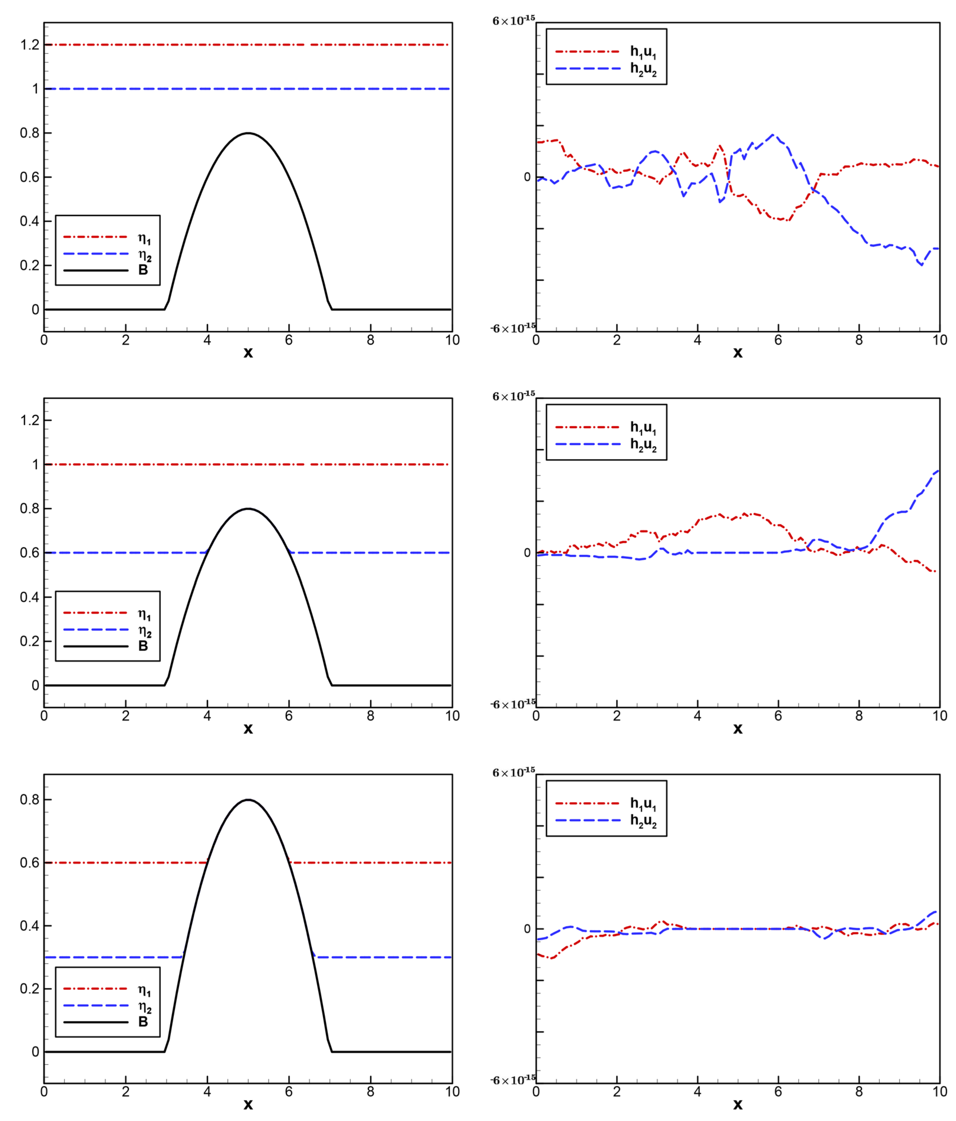
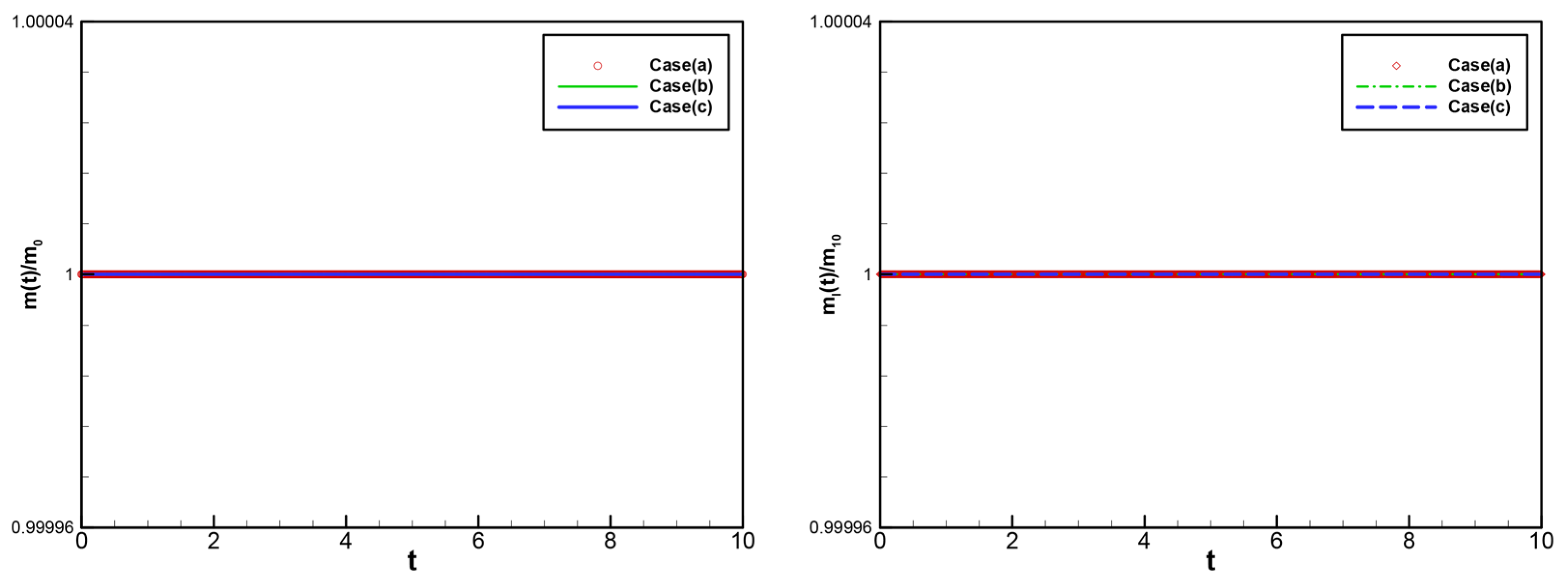
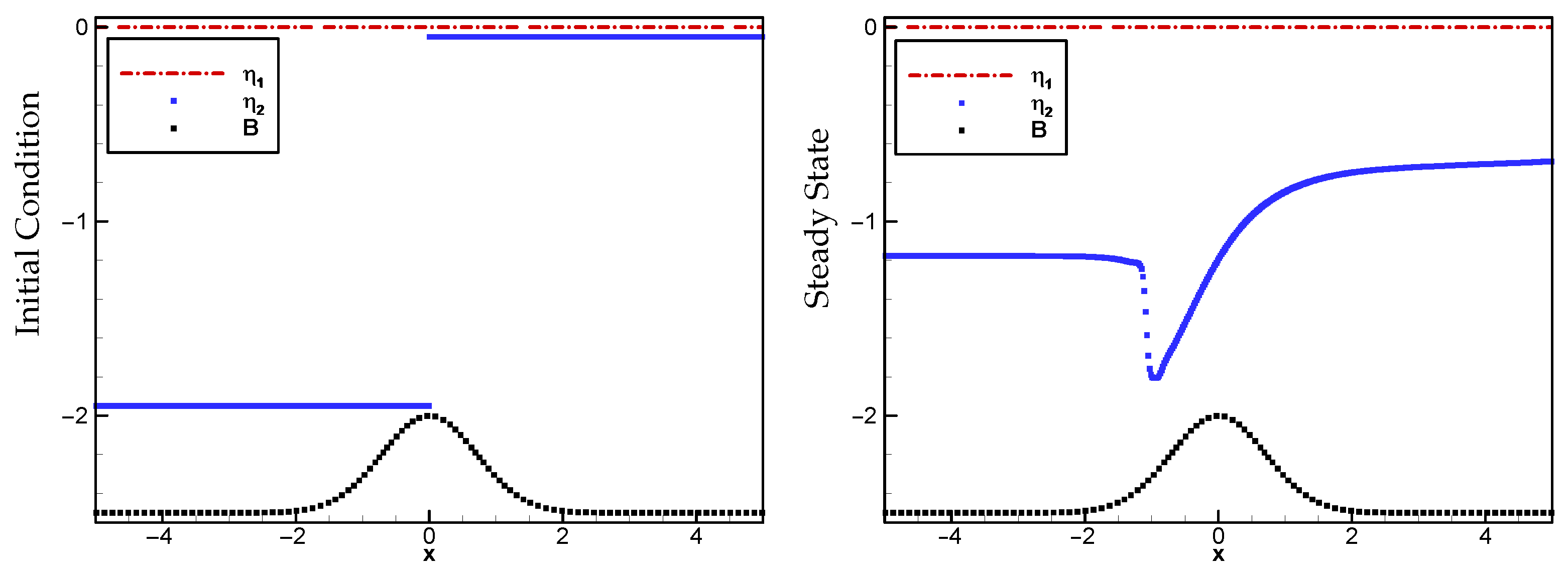
6.2. Stationary Steady-State Solutions
- (a)
- Upper layer: fully flooded; Lower layer: fully flooded,
- (b)
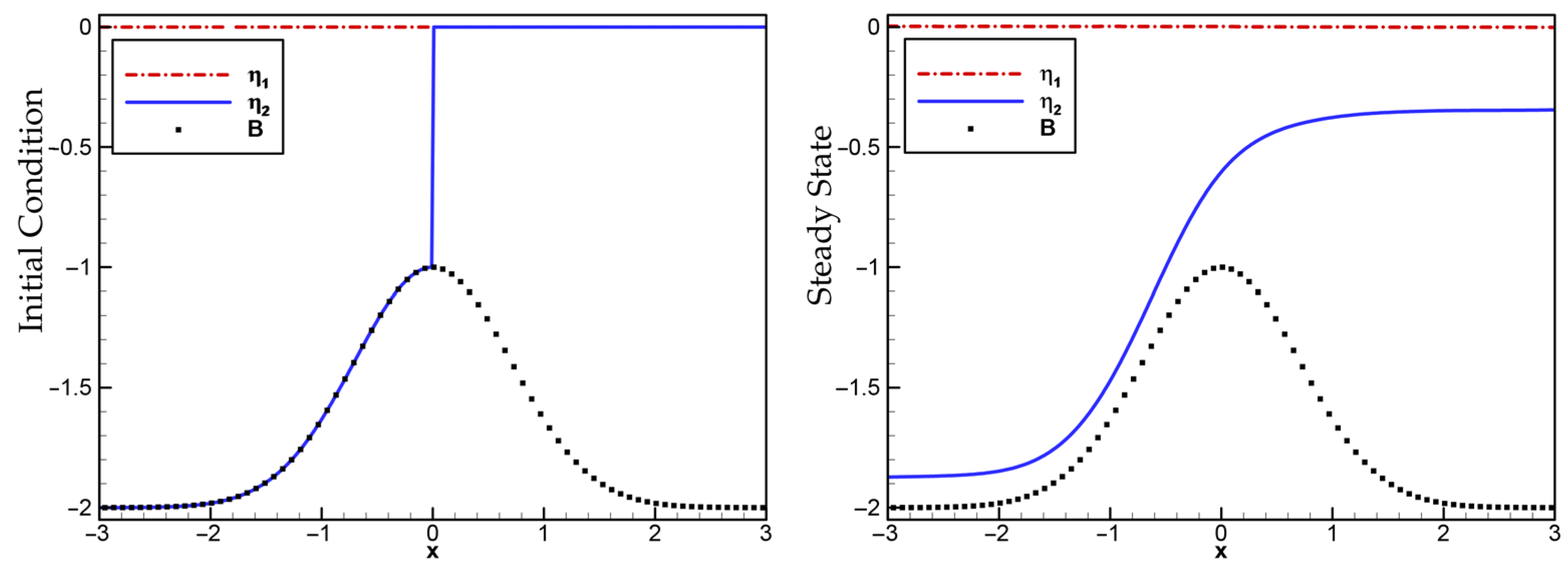
- Upper layer: fully flooded; Lower layer: partially flooded,
- (c)
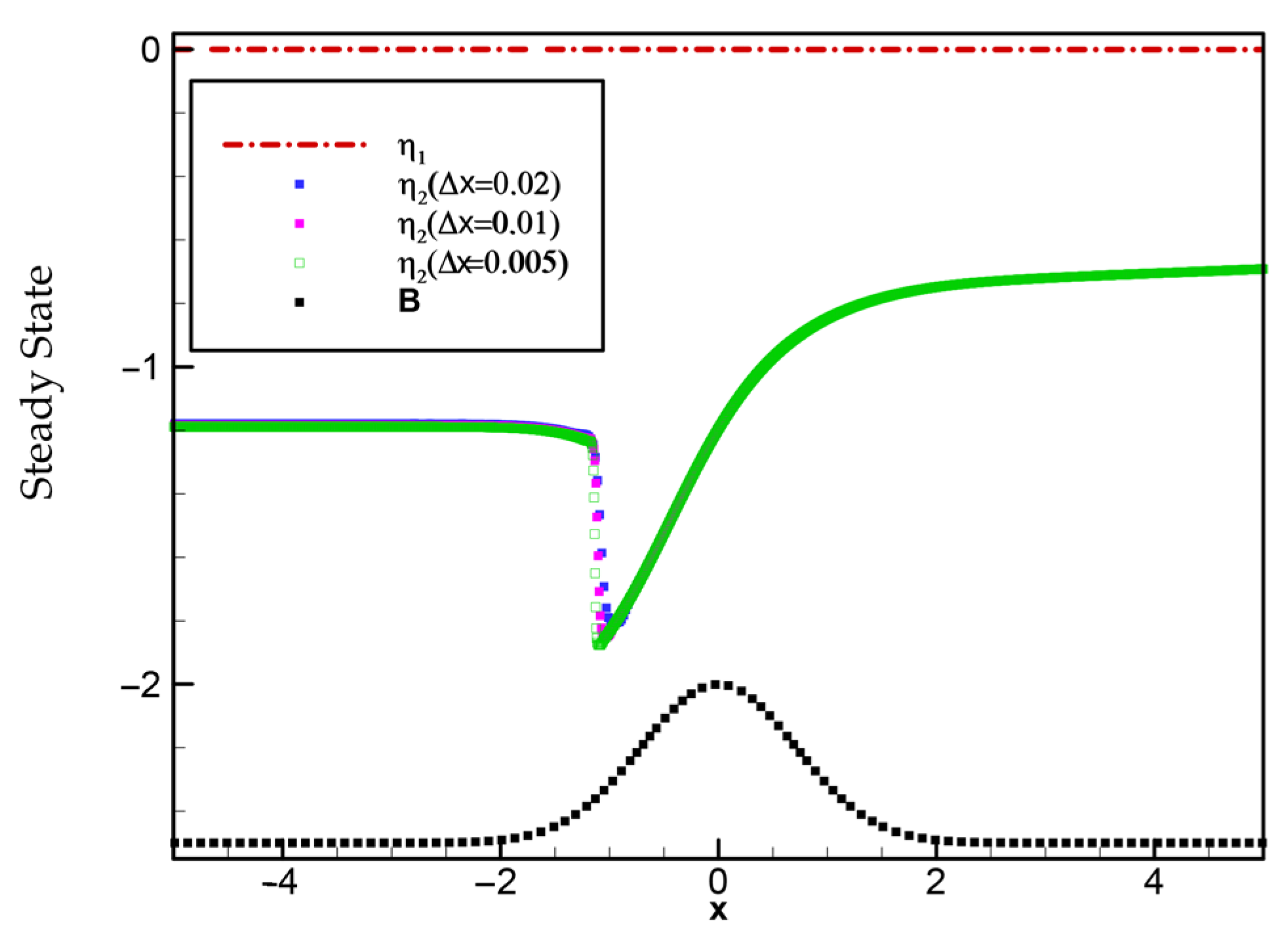
- Upper layer: partially flooded; Lower layer: partially flooded,
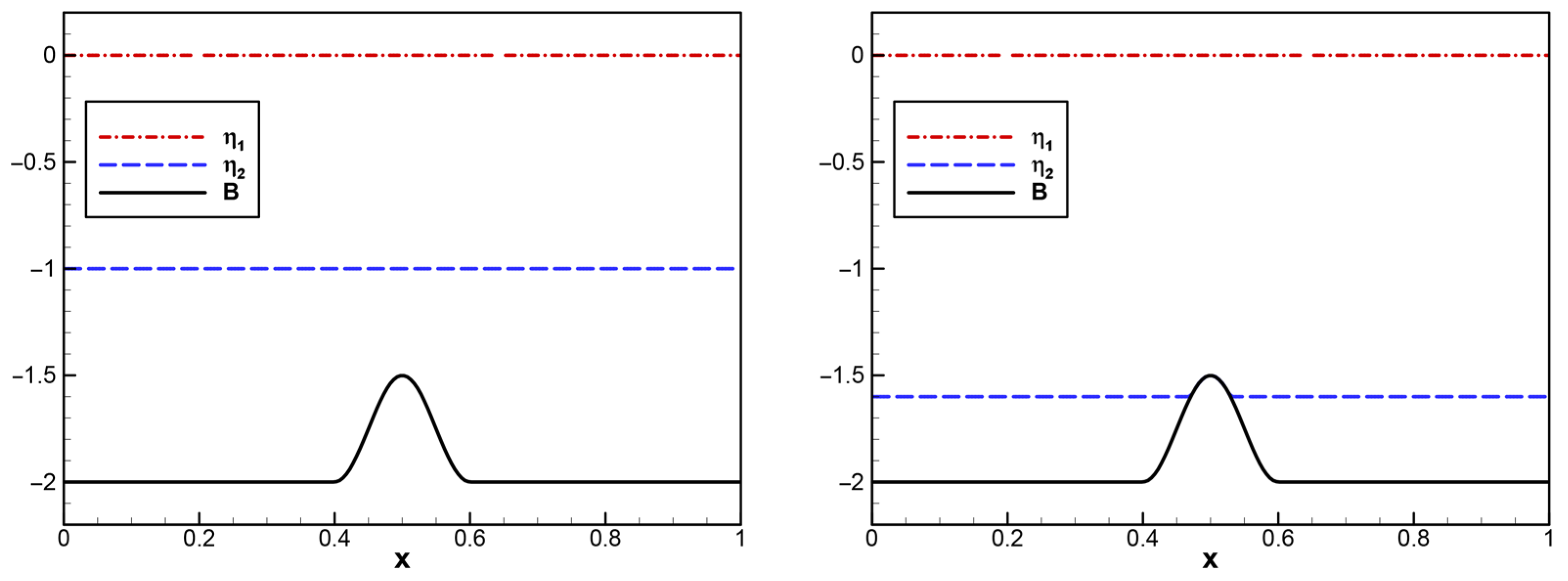
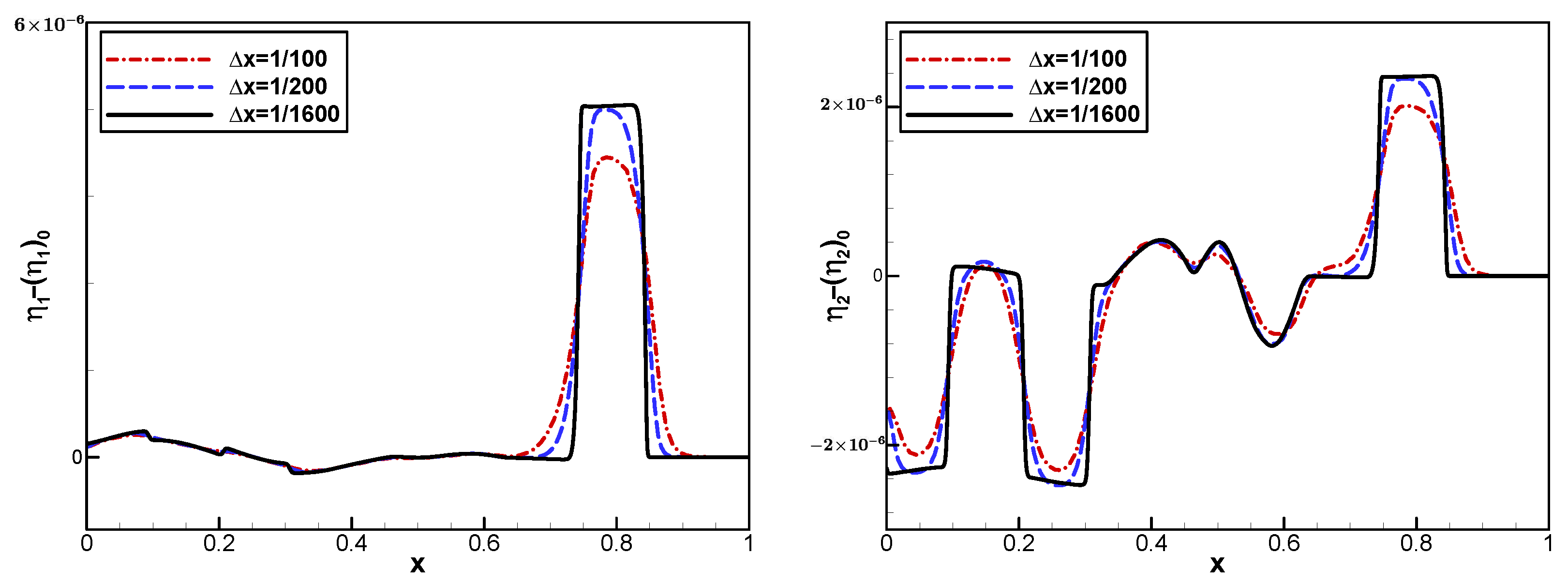
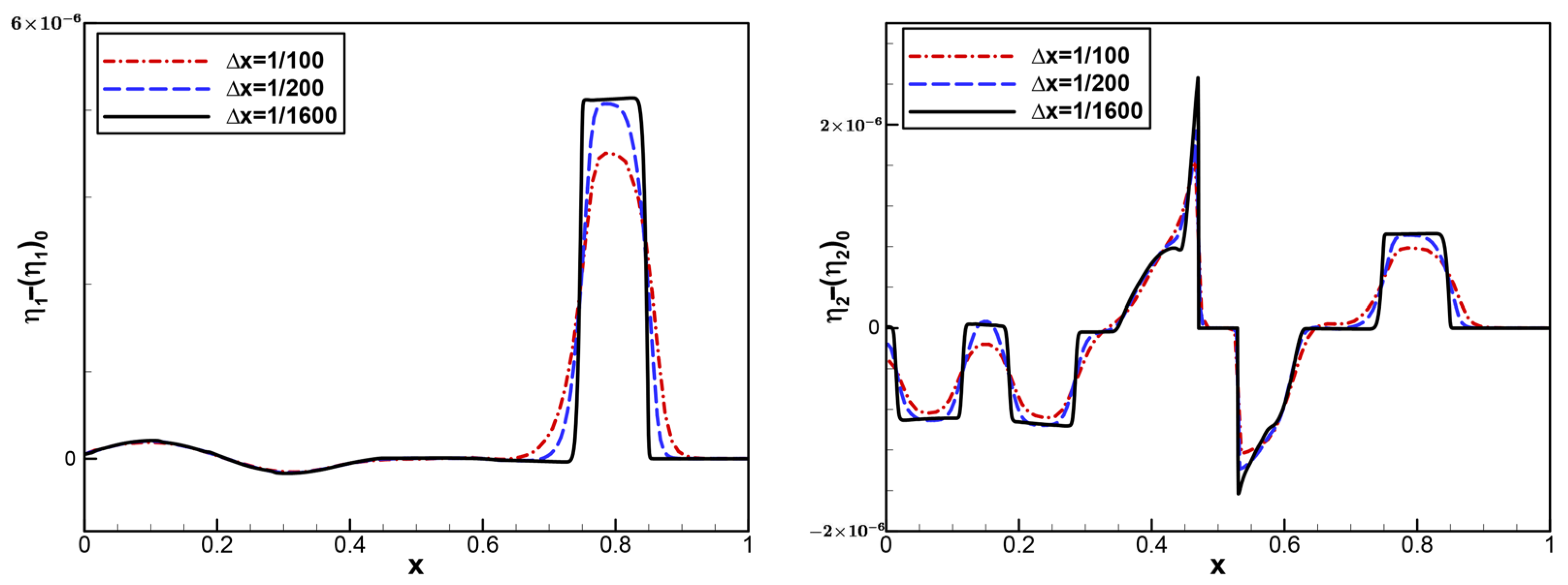
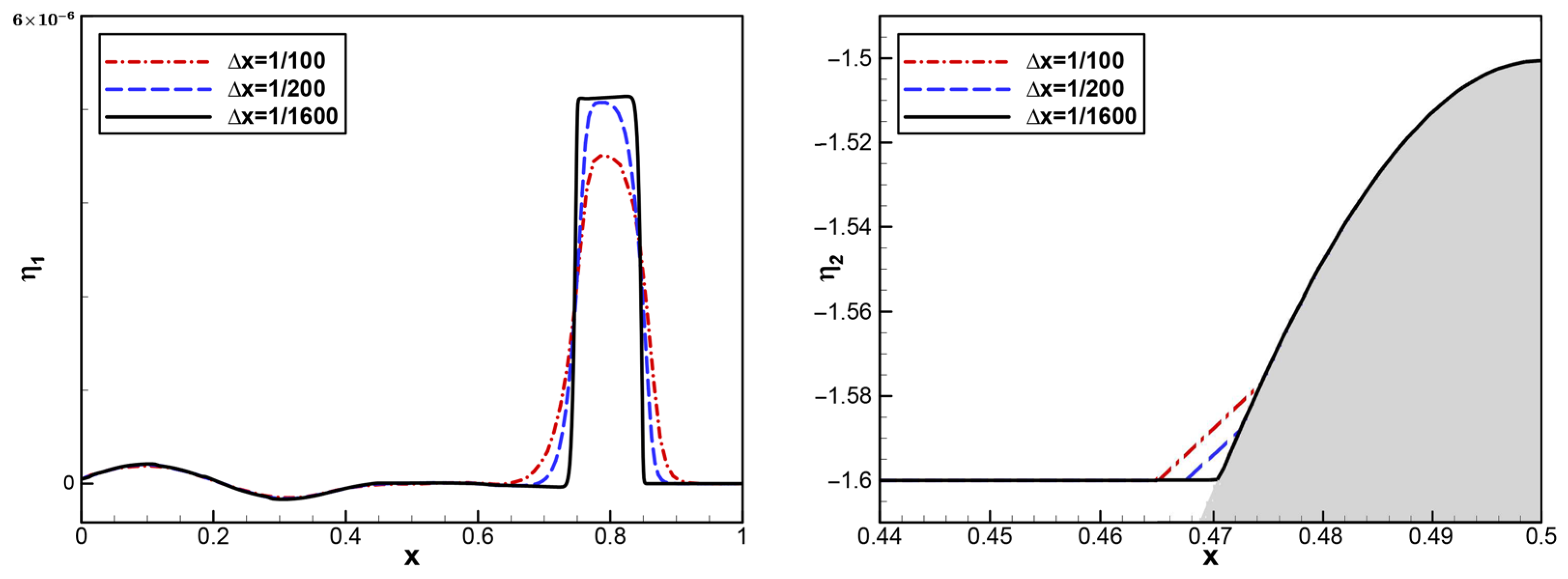
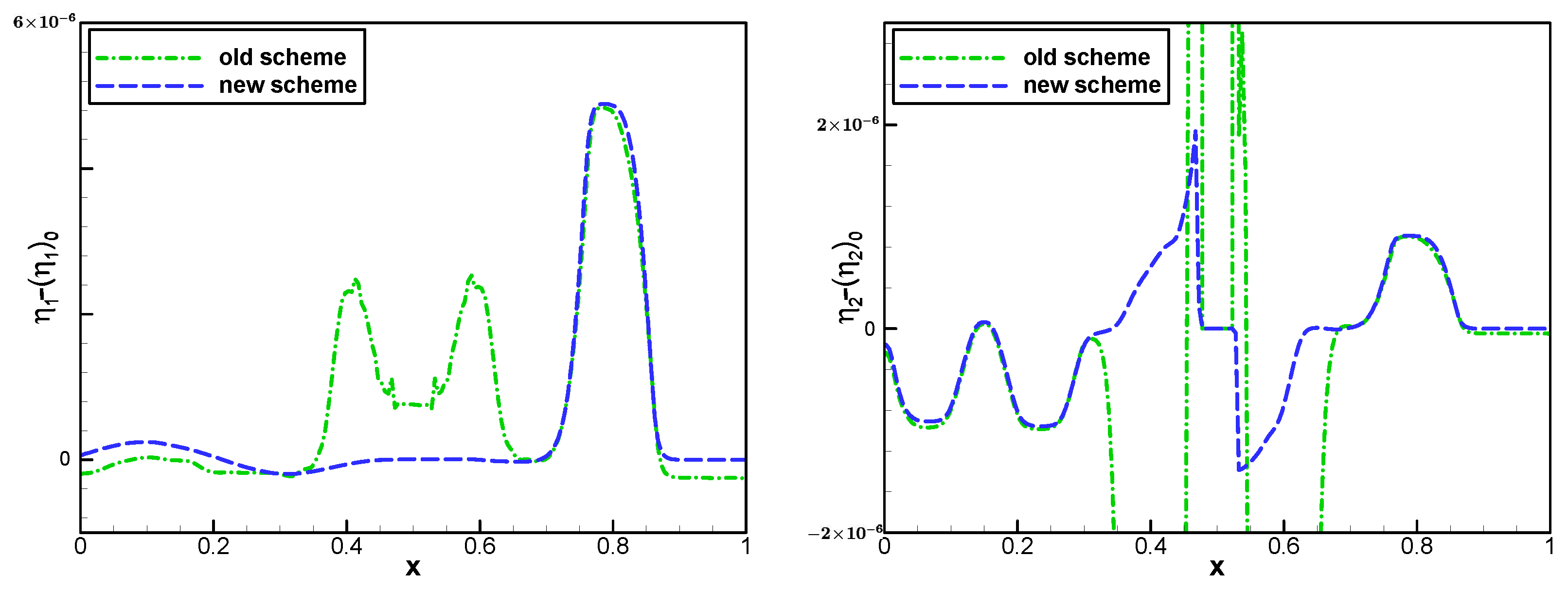
6.3. Small Perturbation of Steady-State Solutions
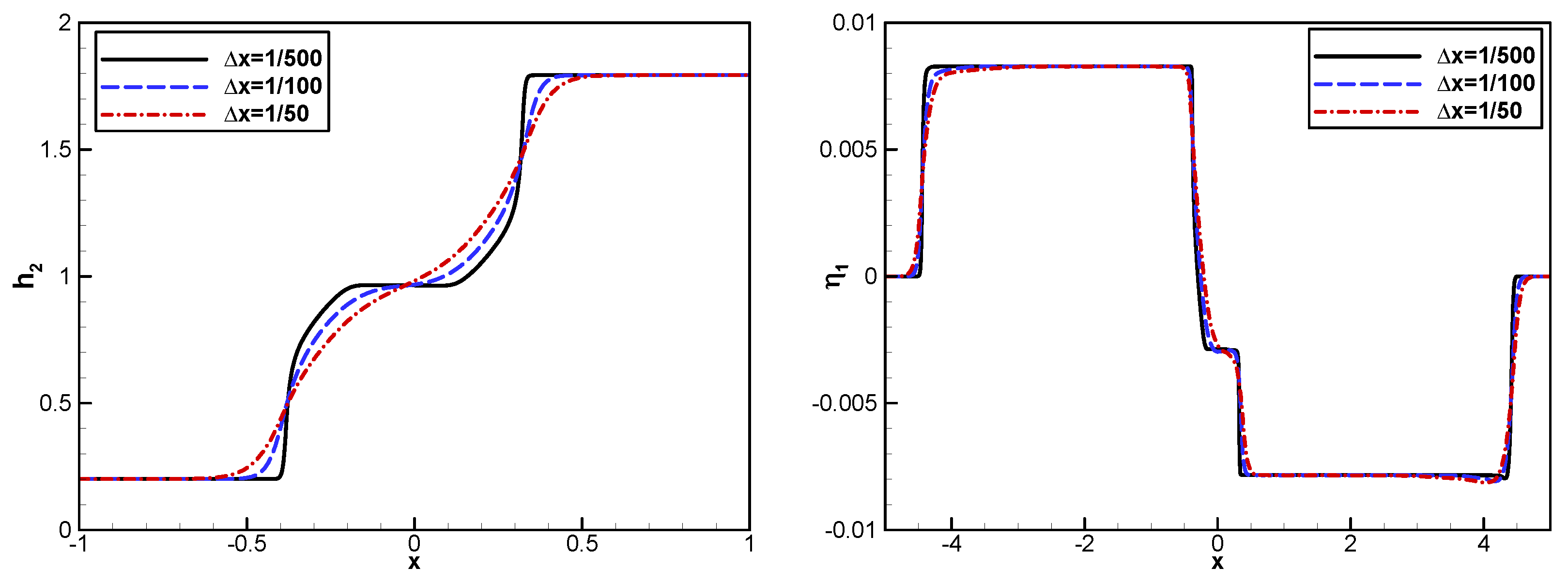
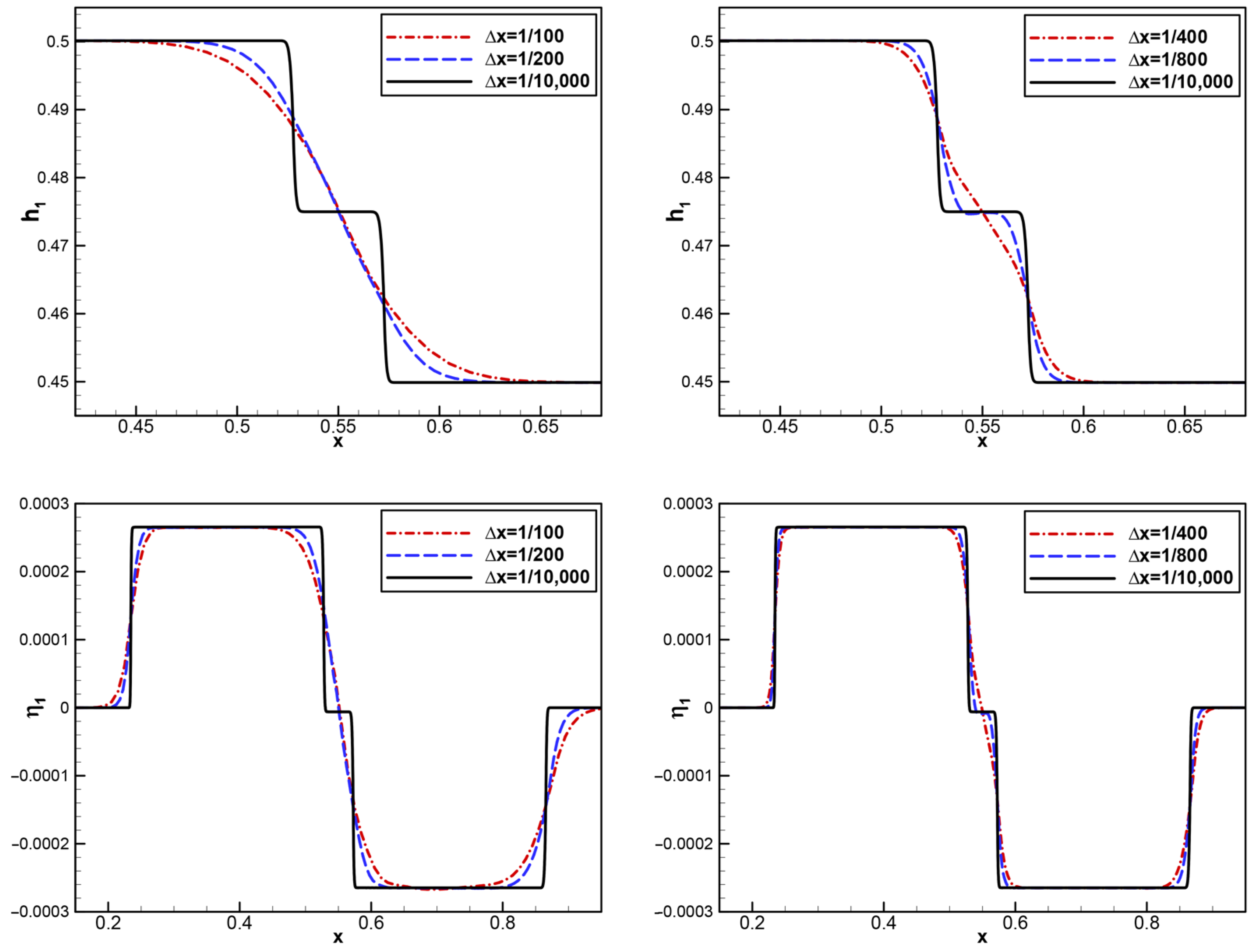
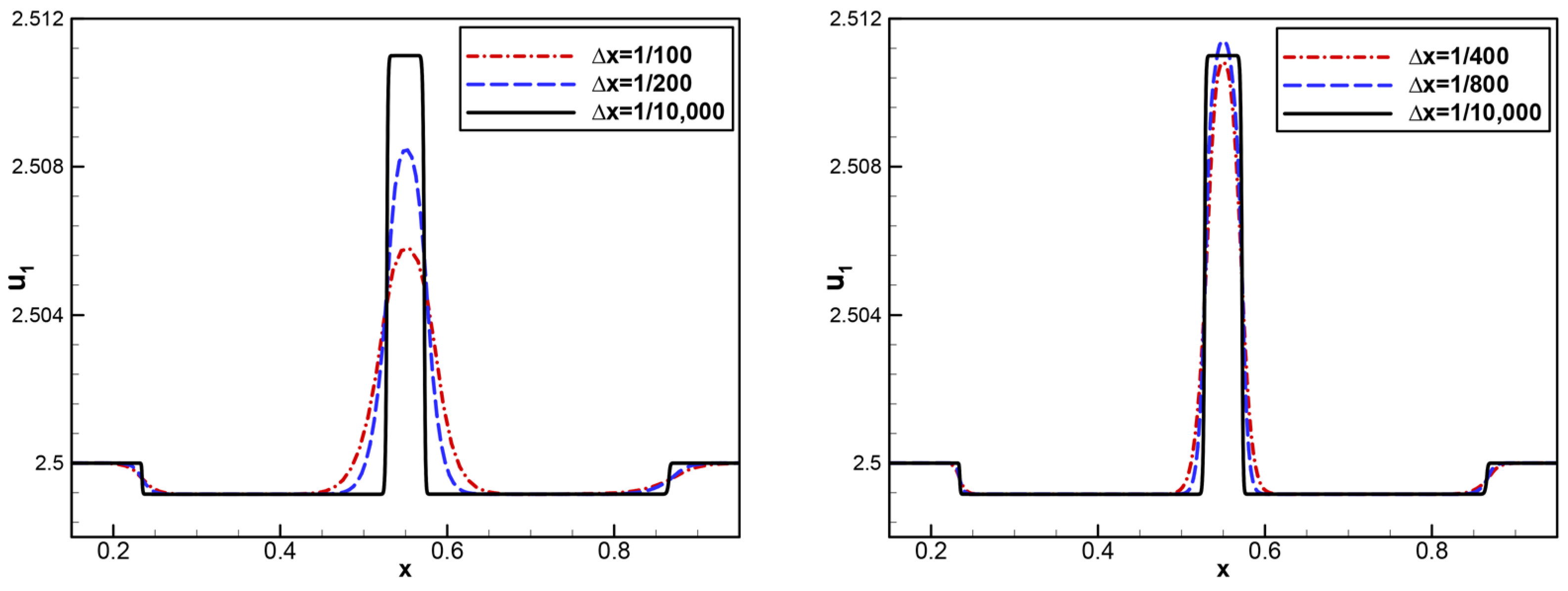
6.4. Interface Propagation
6.5. Lock Exchange Problem
6.6. Internal Dam Break
7. Conclusions
Funding
Data Availability Statement
Acknowledgments
Conflicts of Interest
References
- De St Venant, B. Theorie du mouvement non-permanent des eaux avec application aux crues des rivers et a l’introduction des marees dans leur lit. Acad. Sci. Comptes Redus 1871, 73, 148–154. [Google Scholar]
- Mahdi, T.F. One-Dimensional Shallow Water Equations Ill-Posedness. Mathematics 2025, 13, 2476. [Google Scholar] [CrossRef]
- Castro, M.; Macías, J.; Parés, C. A q-scheme for a class of systems of coupled conservation laws with source term. application to a two-layer 1-d shallow water system. ESAIM Math. Model. Numer. Anal. 2001, 35, 107–127. [Google Scholar] [CrossRef]
- Abgrall, R.; Karni, S. Two-layer shallow water system: A relaxation approach. SIAM J. Sci. Comput. 2009, 31, 1603–1627. [Google Scholar] [CrossRef]
- Bouchut, F.; de Luna, T.M. An entropy satisfying scheme for two-layer shallow water equations with uncoupled treatment. ESAIM Math. Model. Numer. Anal. 2008, 42, 683–698. [Google Scholar] [CrossRef]
- Castro, M.J.; Macıas, J.; Parés, C.; Garcıa-Rodrıguez, J.A.; Vázquez-Cendón, E. A two-layer finite volume model for flows through channels with irregular geometry: Computation of maximal exchange solutions: Application to the strait of gibraltar. Commun. Nonlinear Sci. Numer. Simul. 2004, 9, 241–249. [Google Scholar] [CrossRef]
- Castro Díaz, M.; Chacón Rebollo, T.; Fernández-Nieto, E.D.; Parés, C. On well-balanced finite volume methods for nonconservative nonhomogeneous hyperbolic systems. SIAM J. Sci. Comput. 2007, 29, 1093–1126. [Google Scholar] [CrossRef]
- Dong, J.; Qian, X.; Wei, Z. A robust structure-preserving surface reconstruction scheme for two-layer shallow water equations based on a relaxation model and an extension on adaptive moving triangles. J. Comput. Phys. 2025, 541, 114328. [Google Scholar] [CrossRef]
- Del Grosso, A.; Díaz, M.C.; Chalons, C.; de Luna, T.M. On well-balanced implicit-explicit Lagrange-projection schemes for two-layer shallow water equations. Appl. Math. Comput. 2023, 442, 127702. [Google Scholar] [CrossRef]
- Maso, G.D.; Lefloch, P.G.; Murat, F. Definition and weak stability of nonconservative products. J. De Math. Pures Appl. 1995, 74, 483–548. [Google Scholar]
- Mohamed, K. A modified rusanov method for simulating two-layer shallow water flows with irregular topography. Comput. Appl. Math. 2024, 43, 136. [Google Scholar] [CrossRef]
- Mohamed, K.; Sahmim, S.; Benkhaldoun, F.; Abdelrahman, M.A. Some recent finite volume schemes for one and two layers shallow water equations with variable density. Math. Methods Appl. Sci. 2023, 46, 12979–12995. [Google Scholar] [CrossRef]
- Zhao, F.; Gan, J.; Xu, K. High-order compact gas-kinetic scheme for two-layer shallow water equations on unstructured mesh. J. Comput. Phys. 2024, 498, 112651. [Google Scholar] [CrossRef]
- Du, C.; Li, M. A high-order domain preserving DG method for the two-layer shallow water equations. Comput. Fluids 2024, 269, 106140. [Google Scholar] [CrossRef]
- Guerrero Fernandez, E.; Castro-Diaz, M.J.; Morales de Luna, T. A second-order well-balanced finite volume scheme for the multilayer shallow water model with variable density. Mathematics 2020, 8, 848. [Google Scholar] [CrossRef]
- Castro, M.J.; LeFloch, P.G.; Muñoz-Ruiz, M.L.; Parés, C. Why many theories of shock waves are necessary: Convergence error in formally path-consistent schemes. J. Comput. Phys. 2008, 227, 8107–8129. [Google Scholar] [CrossRef]
- Diaz, M.J.C.; Kurganov, A.; de Luna, T.M. Path-conservative central-upwind schemes for nonconservative hyperbolic systems. ESAIM Math. Model. Numer. Anal. 2019, 53, 959–985. [Google Scholar] [CrossRef]
- Dumbser, M.; Hidalgo, A.; Zanotti, O. High order space–time adaptive ader-weno finite volume schemes for non-conservative hyperbolic systems. Comput. Methods Appl. Mech. Eng. 2014, 268, 359–387. [Google Scholar] [CrossRef]
- Muñoz-Ruiz, M.L.; Parés, C. On the convergence and well-balanced property of path-conservative numerical schemes for systems of balance laws. J. Sci. Comput. 2011, 48, 274–295. [Google Scholar] [CrossRef]
- Parés, C. Numerical methods for nonconservative hyperbolic systems: A theoretical framework. SIAM J. Numer. Anal. 2006, 44, 300–321. [Google Scholar] [CrossRef]
- Kurganov, A.; Petrova, G. Central-upwind schemes for two-layer shallow water equations. SIAM J. Sci. Comput. 2009, 31, 1742–1773. [Google Scholar] [CrossRef]
- Kurganov, A.; Tadmor, E. New high-resolution central schemes for nonlinear conservation laws and convection–diffusion equations. J. Comput. Phys. 2000, 160, 241–282. [Google Scholar] [CrossRef]
- Kurganov, A.; Lin, C.T. On the reduction of numerical dissipation in central-upwind schemes. Commun. Comput. Phys. 2007, 2, 141–163. [Google Scholar]
- Kurganov, A.; Noelle, S.; Petrova, G. Semidiscrete central-upwind schemes for hyperbolic conservation laws and hamilton–jacobi equations. SIAM J. Sci. Comput. 2001, 23, 707–740. [Google Scholar] [CrossRef]
- Kurganov, A.; Tadmor, E. Solution of two-dimensional Riemann problems for gas dynamics without Riemann problem solvers. Numer. Methods Partial. Differ. Equ. Int. J. 2002, 18, 584–608. [Google Scholar] [CrossRef]
- Ahmadi, N. Revolutionizing heat exchanger design: Helical groove turbulators for superior thermal-hydraulic and exergy performance. Results Eng. 2025, 28, 107207. [Google Scholar] [CrossRef]
- Bollermann, A.; Chen, G.; Kurganov, A.; Noelle, S. A well-balanced reconstruction of wet/dry fronts for the shallow water equations. J. Sci. Comput. 2013, 56, 267–290. [Google Scholar] [CrossRef]
- Bollermann, A.; Noelle, S.; Lukáčová-Medvidová, M. Finite volume evolution galerkin methods for the shallow water equations with dry beds. Commun. Comput. Phys. 2011, 10, 371–404. [Google Scholar] [CrossRef]
- Wang, X.; Chen, G. A positivity-preserving well-balanced wet-dry front reconstruction for shallow water equations on rectangular grids. Appl. Numer. Math. 2024, 198, 295–317. [Google Scholar] [CrossRef]
- Wang, X.; Chen, G. Well-balanced and positivity-preserving wet-dry front reconstruction scheme for Ripa models. Appl. Numer. Math. 2025, 213, 38–60. [Google Scholar] [CrossRef]
- Kurganov, A.; Petrova, G. A second-order well-balanced positivity preserving central-upwind scheme for the saint-venant system. Commun. Math. Sci. 2007, 5, 133–160. [Google Scholar] [CrossRef]
- Gottlieb, S.; Shu, C.W.; Tadmor, E. Strong stability-preserving high-order time discretization methods. SIAM Rev. 2001, 43, 89–112. [Google Scholar] [CrossRef]
- Liu, X.; He, J. A well-balanced numerical model for depth-averaged two-layer shallow water flows. Comput. Appl. Math. 2021, 40, 311. [Google Scholar] [CrossRef]
- Hao, J.W.; Caraballo, T. Solvability and convergence results for the temperature and concentration field in incompressible Navier-Stokes equations with boundary conditions. J. Differ. Equ. 2026, 450, 113735. [Google Scholar] [CrossRef]







| Correction Step | Type | Corresponding Equations |
|---|---|---|
| Step 1 | Type 1 | (24)–(26) |
| Type 2 | (27)–(30), (32) | |
| Type 3 | (33) | |
| Step 2 | Type 4 | (34)–(37) |
| Type 5 | (38)–(42), (45)–(46) | |
| Type 6 | (47) |
| N | - | Rate | - | Rate |
|---|---|---|---|---|
| 100 | 1.4223 × 10⁻³ | 1.3806 × 10⁻³ | ||
| 200 | 2.7070 × 10⁻⁴ | 2.39 | 2.5451 × 10⁻⁴ | 2.44 |
| 400 | 5.9511 × 10⁻⁵ | 2.19 | 5.4740 × 10⁻⁵ | 2.22 |
| 800 | 1.2358 × 10⁻⁵ | 2.27 | 1.1186 × 10⁻⁵ | 2.29 |
| 1600 | 2.7100 × 10⁻⁶ | 2.19 | 2.4134 × 10⁻⁶ | 2.21 |
| 3200 | 6.1624 × 10⁻⁷ | 2.14 | 5.4235 × 10⁻⁷ | 2.15 |
| N | - | Rate | - | Rate |
|---|---|---|---|---|
| 100 | 2.0231 × 10⁻³ | 1.7642 × 10⁻³ | ||
| 200 | 3.9979 × 10⁻⁴ | 2.34 | 3.4277 × 10⁻⁴ | 2.36 |
| 400 | 7.3842 × 10⁻⁵ | 2.44 | 6.5734 × 10⁻⁵ | 2.38 |
| 800 | 1.3989 × 10⁻⁵ | 2.40 | 1.3347 × 10⁻⁵ | 2.30 |
| 1600 | 2.9863 × 10⁻⁶ | 2.23 | 2.9129 × 10⁻⁶ | 2.20 |
| 3200 | 6.6795 × 10⁻⁷ | 2.16 | 6.6179 × 10⁻⁷ | 2.14 |
| -Error | -Error | -Error | -Error | -Error | -Error | -Error | -Error | |
|---|---|---|---|---|---|---|---|---|
| Case (a) | ||||||||
| 0 | 0 | 0 | 0 | 5.84 × 10⁻¹⁷ | 1.16 × 10⁻¹⁶ | 2.13 × 10⁻¹⁶ | 7.14 × 10⁻¹⁶ | |
| 9.72 × 10⁻¹⁷ | 1.56 × 10⁻¹⁶ | 2.65 × 10⁻¹⁷ | 2.21 × 10⁻¹⁶ | 1.41 × 10⁻¹⁶ | 5.09 × 10⁻¹⁶ | 3.40 × 10⁻¹⁶ | 1.27 × 10⁻¹⁵ | |
| 2.34 × 10⁻¹⁶ | 1.46 × 10⁻¹⁵ | 1.21 × 10⁻¹⁶ | 1.53 × 10⁻¹⁵ | 2.76 × 10⁻¹⁶ | 1.17 × 10⁻¹⁵ | 1.04 × 10⁻¹⁵ | 3.73 × 10⁻¹⁵ | |
| Case (b) | ||||||||
| 1.13 × 10⁻¹⁷ | 1.13 × 10⁻¹⁶ | 0 | 0 | 3.38 × 10⁻¹⁷ | 1.58 × 10⁻¹⁶ | 4.64 × 10⁻¹⁷ | 1.79 × 10⁻¹⁶ | |
| 7.08 × 10⁻¹⁷ | 4.44 × 10⁻¹⁶ | 7.88 × 10⁻¹⁷ | 3.33 × 10⁻¹⁶ | 2.04 × 10⁻¹⁶ | 6.19 × 10⁻¹⁶ | 2.13 × 10⁻¹⁶ | 7.98 × 10⁻¹⁶ | |
| 4.86 × 10⁻¹⁶ | 1.45 × 10⁻¹⁵ | 1.79 × 10⁻¹⁶ | 9.98 × 10⁻¹⁶ | 8.78 × 10⁻¹⁶ | 2.86 × 10⁻¹⁵ | 8.61 × 10⁻¹⁶ | 3.93 × 10⁻¹⁵ | |
| Case (c) | ||||||||
| 4.14 × 10⁻¹⁸ | 4.14 × 10⁻¹⁷ | 0 | 0 | 2.57 × 10⁻¹⁷ | 6.07 × 10⁻¹⁷ | 8.43 × 10⁻¹⁷ | 2.82 × 10⁻¹⁶ | |
| 5.35 × 10⁻¹⁷ | 1.64 × 10⁻¹⁶ | 4.77 × 10⁻¹⁷ | 1.64 × 10⁻¹⁶ | 1.55 × 10⁻¹⁶ | 3.19 × 10⁻¹⁶ | 1.41 × 10⁻¹⁶ | 5.82 × 10⁻¹⁶ | |
| 1.73 × 10⁻¹⁶ | 7.20 × 10⁻¹⁶ | 1.08 × 10⁻¹⁶ | 6.12 × 10⁻¹⁶ | 4.08 × 10⁻¹⁶ | 1.81 × 10⁻¹⁵ | 3.69 × 10⁻¹⁶ | 1.87 × 10⁻¹⁵ | |
| Scheme | - | - |
|---|---|---|
| Case (a) | ||
| old scheme | 5.04 × 10⁻¹⁶ | 2.24 × 10⁻¹⁵ |
| new scheme | 5.09 × 10⁻¹⁶ | 1.27 × 10⁻¹⁵ |
| Case (b) | ||
| old scheme | 5.18 × 10⁻⁵ | 4.83 × 10⁻⁵ |
| new scheme | 6.19 × 10⁻¹⁶ | 7.98 × 10⁻¹⁶ |
| Case (c) | ||
| old scheme | 6.01 × 10⁻⁴ | 6.98 × 10⁻⁴ |
| new scheme | 3.19 × 10⁻¹⁶ | 5.82 × 10⁻¹⁶ |
| Test Case | Old Scheme (CPU Time, s) | New Scheme (CPU Time, s) |
|---|---|---|
| Case (a) | 0.03102 | 0.03125 |
| Case (b) | 0.04605 | 0.04688 |
| Case (c) | 0.0612 | 0.0625 |
Disclaimer/Publisher’s Note: The statements, opinions and data contained in all publications are solely those of the individual author(s) and contributor(s) and not of MDPI and/or the editor(s). MDPI and/or the editor(s) disclaim responsibility for any injury to people or property resulting from any ideas, methods, instructions or products referred to in the content. |
© 2026 by the author. Licensee MDPI, Basel, Switzerland. This article is an open access article distributed under the terms and conditions of the Creative Commons Attribution (CC BY) license.
Share and Cite
Wang, X. A Well-Balanced Wet–Dry Front Reconstruction for Two-Layer Shallow Water Flows. Mathematics 2026, 14, 595. https://doi.org/10.3390/math14040595
Wang X. A Well-Balanced Wet–Dry Front Reconstruction for Two-Layer Shallow Water Flows. Mathematics. 2026; 14(4):595. https://doi.org/10.3390/math14040595
Chicago/Turabian StyleWang, Xue. 2026. "A Well-Balanced Wet–Dry Front Reconstruction for Two-Layer Shallow Water Flows" Mathematics 14, no. 4: 595. https://doi.org/10.3390/math14040595
APA StyleWang, X. (2026). A Well-Balanced Wet–Dry Front Reconstruction for Two-Layer Shallow Water Flows. Mathematics, 14(4), 595. https://doi.org/10.3390/math14040595