Article

Algorithms for Solving Systems of Boolean Equations Based on the Transformation of Logical Expressions


by
Anvar Kabulov
1,2,†,
Alimdzhan Babadzhanov
3,†,
Abdussattar Baizhumanov
4,†,
Islambek Saymanov
1,5,*,† and
Akbarjon Babadjanov
6,†
1
School of Mathematics and Natural Sciences, New Uzbekistan University, Movarounnahr 1, Tashkent 100007, Uzbekistan
2
Applied Mathematics and Intelligent Technologies Faculty, National University of Uzbekistan, Tashkent 100174, Uzbekistan
3
Department of Algorithmization, Engineering Federation of Uzbekistan, Tashkent 100003, Uzbekistan
4
Department of Mathematics, O. Zhanibekov South Kazakhstan State Pedagogical University, A. Baitursynov Street No. 13, Shymkent 160012, Kazakhstan
5
Department of Applied Informatics, Kimyo International University in Tashkent, Shota Rustaveli Str. 156, Tashkent 100121, Uzbekistan
6
Department of Information Systems, University of Maryland, Baltimore County, 1000 Hilltop Circle, Baltimore, MD 21250, USA
*
Author to whom correspondence should be addressed.
These authors contributed equally to this work.
Mathematics 2026, 14(4), 594; https://doi.org/10.3390/math14040594
Submission received: 12 January 2026 / Revised: 29 January 2026 / Accepted: 5 February 2026 / Published: 8 February 2026

Abstract

This manuscript proves specific theorems for transforming Boolean expressions of logical formulas when moving from one basis to another, simplifying the solution of complex equations, especially for cryptographic applications. The paper develops methods for solving specific nonlinear systems of Boolean equations used in cryptographic S-boxes using transformations to simpler forms, such as disjunctive normal forms (DNFs) and Zhegalkin polynomials. The main contributions include a mathematical basis for transforming formulas, a complexity-reducing grouping method, and the RLSY program for practical implementation. A rigorous theory, cryptographic relevance, and a detailed description of the algorithm are proposed. The grouping method reduces the system complexity by a factor of 2 11 , as shown in a test example, improving computational efficiency. A solution to a special class of systems of nonlinear Boolean equations of the second degree, which are a logical model of algebraic cryptanalysis, is also proposed. Test examples of logical formula transformations are given.

1. Introduction

Algebraic-logical methods are traditionally applied in solving a wide range of problems in pattern recognition theory, neural structure theory, intelligence theory, and mathematical linguistics [1,2,3,4,5]. These methods serve as both a means of formalization and an effective tool for solving the problems that arise in these fields [2,6,7].
We will outline some of the methods used in logical operations when solving systems of logical equations and finding their solutions. As is well known, logical problems are primarily presented in the form of analytical formulas with arbitrary bases [8,9]. It is evident that performing any operation on these formulas is difficult, even with the help of computers. Therefore, we now examine some of the main methods commonly used in logical operations within logical propositions and explore the criteria for transforming logical formulas when transitioning from one base to another [10,11,12,13].
The solution of systems of second-degree nonlinear Boolean equations, which serve as a logical model for algebraic cryptanalysis, is investigated. Test examples of logical formula transformations are constructed [14,15,16,17,18]. The solution of systems of second-degree nonlinear Boolean equations of a special class is considered. The advantage of the research results compared to others lies in the ability to solve systems of special second-degree nonlinear Boolean equations based on grouping and minimizing logical propositions in the disjunctive normal form (DNF) class [19]. These equations serve as the algebraic model of S-blocks in symmetric encryption algorithms [5,20,21,22].

2. Criteria for Analytical Transformations of Boolean Expressions

It is easy to notice that when performing successive elementary transformations, the number of different logical operations increases significantly, requiring enormous computational resources. We will present several formulas in which logical transformations frequently occur, determining a direct transition from one expression to another, as well as the apparatus of decimal numbers, which can be easily implemented on computers [23,24,25,26,27,28].
Let us introduce the following notation: i = 1 m ,   i = 1 m ,   i = 1 m , i = 1 m ,   / / i = 1 m ,   i = 1 m refer to m-fold equivalence, disjunction, conjunction, modulo 2 addition ( mod 2 ), Sheffer’s operation, and implication.
Let us denote by E n 2 the set of all binary vectors α 1 , α 2 ,   ,   α n . It can be considered as the set of all vertices of a unit n-dimensional cube, with the vectors α 1 , α 2 ,   ,   α n representing the vertices of the cube [29,30,31,32].
Defination 1.
The i-th level of a cube is defined as the set of tuples in E n 2 whose number of unit coordinates is equal to i, where i = 0 ,   1 ,   ,   n .

3. Methods of Boolean Formula Transformations for Simplifying Logical Statements

We consider analytical criteria for transformation that examine the issues of converting formulas from an arbitrary basis ( { ¬ x ,   x 1   &   x 2 ,   x 1 x 2 ,   x 1 x 2 , x 1 x 2 ,   x 1 x 2 ,   x 1 / x 2 } ) into formulas over the basis { 0 ,   1 ,   x 1 & x 2 , x 1 x 2 } [33,34,35,36,37].
In what follows, we transform logical formulas through an expression of the form A i o 1 m A i * o 2 m 1 , where A i o m = A 1 · A 2 · · A m . We will denote the transformation from the sequential logical operation o 1 to the operation o 2 , where o 1 ,   o 2 are symbols for logical operations; L o 2 o 1 ( m ) is the number of occurrences of variables in A j * o i m 1 ,   i = 1 ,   2 ,   ,   m ; j = 1 ,   2 ,   ,   m 1 ; and m 1 = K o 2 o 1 m is the number of elementary conjunctions in A j * o 2 m 1 ,   A i ,   A j * —elementary conjunctions.
The criteria for transforming formulas are considered here: { U i } m { U j * } m 1 ,   { U i } m { U j * } m 1 ,   { U i } m { U j * } m 1 ,   { U i } I m { U j * } m 1 (this allows for eliminating intermediate results in the transformation process and evaluating their complexity in K o 2 0 1 m ,   L 0 2 0 1 ( m ) ). Additionally, a new approach to transforming formulas from an arbitrary basis to the Zhegalkin polynomial is considered and theoretically justified [38,39].
Theorem 1.
The transformation { U i } / m { U j * } m 1 is uniquely represented in the form of a decomposition modulo 2:
& i = 1 m U i i = 3 m ( & j = i m U j ) 1
or
( 1 U m ( 1 U m 1 ( 1 U m 2 ( 1 U 3 ( 1 U 1 U 2 ) ) ) ) )
where (2) is obtained from (1) by factoring out common arguments and K Σ / m = m , L / ( m ) = Σ i = 1 m 1 i + 1 .
Proof. 
We apply the method of induction:
(a) For m = 2, the following relation holds: U 1 / U 2 U 1 U 2 1 .
(b) For m = 3, we have U 1 / U 2 / U 3 = U 1 U 2 U 3 U 3 1 .
(c) Suppose that relation (2) holds for m = n: // i = 1 n U i ( 1 U n ( 1 U n 1 ( 1 U 3 ( 1 U 1 U 2 ) ) ) ) .
We will prove the validity of relation (2) for m = n + 1 :
// i = 1 n + 1 U i n / / i = 1 U i / U n + 1 ( // i = 1 n U i ) U n + 1 1 ( 1 U n ( 1 U n + 1 ( 1 U 3 ( 1 U 1 U 2 ) ) ) ) U n + 1 1 ( 1 U n + 1 ( 1 U n ( 1 U n 1 ( 1 U 3 ( 1 U 1 U 2 ) ) ) )
From this, we obtain // i = 1 n + 1 U i = 1 U n + 1 ( 1 U n ( 1 U 3 ( 1 U 1 U 2 ) ) ) .
The estimates K Σ / m and L Σ / m are easily derived from Formula (1). □
Theorem 2.
The transformation { U i } m { U j * } m 1 has the form
{ U j * } m 1 = ( U 1 σ 1   &   U 2 σ 2   &     U k σ k )
where ( σ 1 σ 2 σ m = 1 ) ,   { σ 1 ,   σ 2 ,   ,   σ k } { σ 1 ,   σ 2 ,   ,   σ m } ,  σ 1 = σ 2 = = σ k = 1 , i k 1 , 2 , , m , k m , and L Σ V m = Σ i = 1 m ( i · C m i ) , K Σ V m = 2 m 1 .
Proof. 
Let B k and l k denote the expression and the number of unit coordinates after transforming the formulas k i = 1 U i into the Zhegalkin polynomial.
For k = 2 and k = 3 , the formulas are found very easily:
U 1 U 2 = U 1 U 2 U 1 U 2 = B 2 , l 2 = 3 ;
U 1 U 2 U 3 = B 2 U 3 B 2 U 3 = U 1 U 2 U 3 U 1 U 3 U 2 U 3 U 1 U 2 U 1 U 2 U 3 = B 3 , l 3 = l 2 + l 2 + 1 = 7 ;
Let k = n + 1 . Then, the following holds:
U 1 U 2 U n U n + 1 = B n U n + 1 B n U n + 1 , l n + 1 = 2 l n + 1 .
If for B k k = 1 , , n + 1 , the number of unit coordinates is calculated sequentially,
k = 1 , l 1 = 1 = 2 1 1 , k = 2 , l 2 = 2 l 1 + 1 = 3 = 2 2 1 , k = 3 , l 3 = 2 l 2 + 1 = 7 = 2 3 1 , k = n + 1 , l n + 1 = 2 l n + 1 = 2 n + 1 1 .
then it is easy to observe that for m variables, we have l m = K Σ ( m ) = 2 m 1 .
If we consider that E m 2 = 2 m and K Σ m = 2 m 1 , then the decomposition consists of all possible unit elements of an m-dimensional cube, through which Formula (3) can be easily expressed in an analytical form.
It is known that at each level i of the m-dimensional cube, there are C m i sets, and in each set, i units participate, corresponding to m variables. Consequently, the number of variable occurrences in the polynomial { U j } Σ m equals L Σ m = Σ i = 1 m ( i C m i ) . □
Theorem 3.
In the basis D 2 = { 0 ,   1 ,   x 1   &   x 2 ,   x 1 x 2 } , the sequence of implication operations is uniquely represented in the form of a Zhegalkin polynomial:
= 1 m U i = 1 m 2 ( t 2 1 ) j = 2 i m t + 2 k = j + 1 m t + 3 l = n + 1 m ( U 2 i 1 U j U k U l ) i = 1 m 2 ( p 1 ) 2 j = 2 i m p + 2 k = j + 1 m p + 3 l = n + 1 m ( U 2 i 1 U j U k U l )
where
t = 2 , 4 , , m if m is even , 1 , 3 , , m otherwise .
= 1 , 3 , , m 1 ; if m is even , 2 , 4 , , m 1 ; otherwise .
c = 1 , if m is even , 0 , otherwise .
and the following holds:
K Σ m = 1 + 2 3 ( 2 m 1 ) , if m is even , 1 3 ( 2 m + 1 1 ) , otherwise .
where p and t represent the number of arguments in the unit coordinate system.
Proof. 
The proof of the main formula is not provided, as it can be easily obtained using a method similar to that of the previous theorems or through a sequential transformation into the Zhegalkin polynomial. Let us consider the proof of the number of unit coordinates involved in the polynomial for arbitrary m.
Let T i i = 1 , 2 , , m be the number of unit coordinates in the polynomial as the number of variables increases from 1 to m.
For m = 2 and m = 3 , we have
U 1 U 2 = U 1 U 2 U 1 1 ,
U 1 U 2 U 3 = U 1 U 2 U 3 U 1 U 2 U 1 U 3 U 1 U 3
and, consequently, we obtain T 2 = 3 , T 3 = 5 .
If we sequentially construct the polynomials, it is easy to notice that the number of unit coordinates in each subsequent polynomial is either one more or one less than in the previous one. It increases by one if m is even and decreases by one otherwise.
Thus, we can construct a numerical sequence that defines the number of unit coordinates in the polynomial as m increases:
T i = 2 T i 1 + 1 , if i is even , 2 T i 1 1 , otherwise , where i = 2 , 3 , , m
Let us divide the sequence into two groups based on even and odd values of m:
T 2 k : 3 , 11 , 43 , 171 , , k = 1 , 2 , , m / 2 ;
T 2 k 1 : 1 , 5 , 21 , 85 , 341 , , k = 1 , 2 , , m + 1 / 2 .
From this, it is evident that
T 2 k = T 2 ( k 1 ) + 2 2 k 1 and T 2 k 1 = T 2 k 1 1 + 2 2 k 2 or
T 2 k = 1 + 2 1 + 2 3 + 2 5 + + 2 2 k 1 = 1 + 2 ( 1 + 2 1 + 2 4 + + 2 2 k 2 ) = = 1 + 2 ( 1 + 4 1 + 4 2 + + 4 ( k 1 ) ) ;
T 2 k 1 = 2 o + 2 2 + 2 4 + + 2 2 k 2 = 1 + 4 1 + 4 2 + + 4 k 1 .
Using the sum of a geometric progression, we obtain
T 2 k = 1 + 2 ( 4 k 1 4 1 ) = 1 + 2 3 4 k 1 , T 2 k 1 = 4 k 1 / 3 = 1 3 4 k 1
or, considering that 2k = m when m is even, and 2 k 1 = m , 2 k = m + 1 otherwise, along with 4 k = 2 2 k , the following holds:
T m = 1 + 2 3 ( 2 m 1 ) , if m is even 1 3 ( 2 m + 1 1 ) , otherwise .
Theorem 4.
The transformation U i m = U j Σ m can be uniquely represented in the form of a decomposition modulo 2 (mod2).
m i = 1 A i = ¬ i = 1 m U i , if m is even , i = 1 m U i , otherwise .
and
K Σ m = m + 1 , if m is even , m , otherwise . , L Σ m = m .
With this transformation, the inverse problem is also solved in the same manner, i.e.,
i = 1 m U i = m i = 1 U i , if m is even ; m i = 1 U i , otherwise .
Theorem 5.
The transformation { U i } & m = { U j } Σ m 1 in its analytical form is uniquely represented as an expansion in terms of mod2.
¬ U i & m = & i = 1 m   ( ¬ U i ) = & i = 1 m U i i = 1 2 j = i + 1 3 k = l + 1 m U i U j U k i = 1 m 1 j = i + 1 m U i U j i = 1 m U i 1 ;
The proof of the theorem is easily provided using the method of induction.
Let P ( 1 , x 2 , , x n ) = i = 1 k + 1 U i ( 1 , 2 , , n ) be a polynomial over the basis B * , where U i is an elementary component, U l U j , and let U ( σ i 1 , σ i 2 , , σ i k ) denote the elementary component U = x i 1 σ i 1 · x i 2 σ i 2 · · x i k σ i k .
Theorem 6.
The polynomial P ( i 1 , x i 2 , , x i k ) is identically equal to one if P can be represented in the form
U j 1 ( σ i 1 ) U j 2 ( σ ¯ i 1 , σ i 2 ) U j 3 ( σ i 1 ¯ , σ i 2 , ¯ σ i 3 ¯ ) U j k ( σ i 1 ¯ , , σ i k 1 ¯ , σ i k ) U j k + 1 ( σ i 1 ¯ , , σ i k 1 ¯ , σ i k ¯ )
where U j i U i , i = 1 , 2 , , k + 1 ; .
Proof. 
Let us express the polynomial (4) in its general form as follows:
i = 1 k ( & j = 1 i 1 x i j σ i j ¯ ) x i j σ i j j = 1 k x i j σ i j ¯
or
x i 1 σ i 1 x i 1 σ i 1 ¯ x i 2 σ i 2 x i 1 σ i 1 ¯ x i 2 σ i 2 ¯ x i 3 σ i 3 x i 1 σ i 1 ¯ x i k 1 σ i k 1 ¯ x i k σ i k x i 1 σ i 1 ¯ x i k σ i k ¯ .
Corollary 1.
U j 1 U j i 1 U j i + 1 U j k + 1 U j i 1 , holds if U j 1 U j i 1 U j i + 1 U j k + 1 = U j i 1 , satisfies the condition of Formula (4), where U j l , l = 1 , 2 , , k + 1 .
Corollary 2.
If the elementary component U , i = 1 , , m ; G j , j = 1 , , t can be expressed as U = · U , G j = × G j where U , G j (elementary component) and i = 1 m U i = 1 , j = 1 t G j = 1 , then i = 1 m U j = 1 t G j = 0 .

4. Text Example

1. Initial analytical formula: R = R 1 ~ R 2 ~ R 3 ~ R 4 , where R 1 = X 1 & ¬ X 3 & x 5 , R 2 = ¬ X 2 & X 3 & ¬ X 4 & X 5 , R 3 = ¬ X 3 & ¬ X 5 , R 4 = ¬ X 1 & ¬ X 3 & ¬ X 5 (See Table 1).
σ 1 σ 2 σ 3 σ 4 = 1 is the set of tuples satisfying the following equality: Q = 0000 , 0011 , 0101 , 0110 , 1001 , 1010 , 1100 , 1111 .
2. Corresponding disjunctive normal form (DNF)
R = ¬ A 1   &   ¬ A 2   &   ¬ A 3   &   ¬ A 4 v ¬ A 1   &   ¬ A 2 A 3   &   A 4 v ¬ A 1   &   A 2   &   &   ¬ A 3   &   A 4 v v ¬ A 1   &   A 2   &   A 3   &   ¬ A 4 v A 1   &   ¬ A 2   &   ¬ A 3 A 4 v A 1   &   ¬ A 2   &   A 3   &   ¬ A 4 v v A 1   &   A 2   &   ¬ A 3   &   ¬ A 4 v A 1   &   A 2   &   A 3   &   A 4 ;
3. Result of the obtained formula after minimization in the reduced basis.
4. Result in analytical form (See Table 2):
R 2 = X 2 &   X 3 v X 3 &   X 4 v X 3   &   X ¯ 5 v X ¯ 1 &   X 2 &   X 5 v X ¯ 1 &   X 4 &   X 5 v X ¯ 1 &   X ¯ 3

5. Solution of Second-Degree Nonlinear Boolean Equation Systems of a Special Class

This study examines the solution of second-degree nonlinear Boolean equation systems, which serve as a logical model for algebraic cryptanalysis [40]. Test examples of logical formula transformations are constructed. The research also explores the solution of second-degree nonlinear Boolean equation systems of a special class. The key advantage of the findings compared to other approaches lies in the ability to solve such systems based on the grouping and minimization of logical statements in the class of disjunctive normal forms (DNFs), which serve as an algebraic model of S-boxes in symmetric encryption algorithms [41,42,43].
A special class of systems of nonlinear Boolean equations of the second degree is being studied:
R = f 1 x 1 , x 2 , , x n = α 1 , f 2 x 1 , x 2 , , x n = α 2 , , f m x 1 , x 2 , , x n = α m
Moreover, the statement f x 1 , x 2 , , x n from R has the form
f = i , j = k i < j k + 3 a i j x i x j i , j = e i < j e + 3 b i j x i x j i , j = p i < j p + 3 c i j x i x j i , j = q i < j q + 3 d i j x i x j i = t t + 3 e i x i ,
where k + 3 < e , e + 3 < p , p + 3 < q , q + 3 < t ;
i , j = k k + 3 a i j = i , j = e e + 3 b i j = i , j = p p + 3 c i j = i , j = q q + 3 d i j = 4 , a i j , b i j , c i j , d i j , e i 0 , 1
Here, the symbols , Σ are understood as summation modulo 2.
To solve nonlinear Boolean equations of the second degree, the study focuses on compactly representing statements f by grouping elements, introducing new variables, transforming f into specialized disjunctive normal forms (DNFs) using a more optimal decimal representation method, simplifying these specialized DNFs, and analyzing the key features of formula implementation for this special class of nonlinear Boolean equation systems of the second degree.
Here, sums of the form i , j = v v + 3 q i j x i x j and i = w w + 1 e i x i will be referred to as groups of elements of the statement f. Moreover, the groups of different equations (statements) in the system R do not coincide pairwise.
The method for solving system R consists of compactly representing f i by grouping elements, introducing new variables, transforming them into disjunctive normal forms (DNFs), and simplifying them. The search for solutions to system R is carried out using an algorithm for solving systems of linear Boolean equations.
The functional of an arbitrary system α , obtained from R by grouping and replacing variables in the elements of the statements, is denoted as follows:
ψ α = φ y , where Y is the set of variables in system α , φ y is the number of occurrences of Y Y in Y, and Y is the number of elements in Y. The algorithm for grouping system R from the given class consists of the following steps:
Groups of elements of the statements in system R are identified;
All possible groupings within these groups are performed, and new variables are introduced.
From each group, such groupings of elements are selected to ensure that for the resulting system α , the functional ψ α is maximized among all functionals ψ β of systems β formed from the groupings of the system’s groups.
Thus, for a formula like
f = i , j = k i < j k + 3 a i j x i x j i , j = e i < j e + 3 b i j x i x j i , j = p i < j p + 3 c i j x i x j i , j = q i < j q + 3 d i j x i x j i = t t + 3 x i ,
the matrix A n × n is constructed, where the element a i j = 1 if the formula f contains x i x j and a i j = 0 otherwise. Here, a i i corresponds to x i x i in formula f, i.e., x i . Then, the maximum grouping problem in formula f is identical to the problem of finding the maximum identity submatrix of matrix A. It is easy to see that the algorithm for solving the latter problem has polynomial complexity.
It has been proven that at the initial stage, each statement f x 1 , x 2 , , x n from R involves 20 elementary conjunctions. However, after grouping and introducing new variables, the statements F x ˜ , Y x ˜ in the transformed system R * will contain no more than nine linear conjunctions. From this data, based on U 1 U 2 U t = σ 1 σ 2 σ t = 1 U 1 σ 1   &   U 2 σ 2   &     &   U t σ t , we obtain L k f = 2 20 , L k F = 2 9 .
From this, it is evident that the complexity difference between statements f and F is reduced by a factor of 2 11 , i.e., L k = L k f L k F = 2 20 2 9 = 2 11 , where L k Q is the number of elementary conjunctions in the disjunctive normal form (DNF) Q that we obtain.
This means that the method of grouping elements and introducing new variables for second-degree equations of a special class reduces the complexity of Boolean equation statements by a factor of 2 11 .
Solving systems of nonlinear Boolean equations is an N P -complete problem. Moreover, the SAT or Mutant solvers offer a solution to the problem based on posing all binary sets α 1 , α 2 , , α n of the set E n 2 for each equation without simplifying the Boolean equation statements. This increases the complexity of the system / E n 2 / times, where / M / is the cardinality of the set M.
However, the article proposes grouping nonlinear polynomials. Moreover, this is not always the case; in the best case, second-order polynomials can be reduced to a linear polynomial by grouping, demonstrating the transition from the NP problem to the P problem. For example, the equation x 1 x 3 + x 1 x 4 + x 2 x 3 + x 2 x 4 = 1 can be transformed to the equation x 1 + x 2 x 3 + x 4 = 1 , which is identical to the system x 1 + x 2 = 1 , x 3 + x 4 = 1 .
In addition, minimization of statements of nonlinear Boolean equations is performed, for example, in the application of the formula
F ( X ) + 1 = F ( X ) F ( X ) G ( X ) + F ( X ) = F ( X ) G ( X ) + 1 = F ( X ) G ( X )
Let
F 5 F 4 F 3 F 2 F 1 = 1
There are 13 solutions in total (See Table 3).
Example: Solve the equation.
F x 1 , , x 5 = x 1 x 2 x 3 x 4 x 5 + x 3 x 4 x 5 + x 4 x 5 + x 4 = 1 .
It is easy to see that (See Table 4)
x 4 x 5 x 1 x 2 x 3 = 1
There are 11 solutions in total.
The following example can be used as an example of the results for S-boxes. For the GOST R34.12-2015 (Kuznechik) algorithms [44], the S-box ANF consists of y(0), …, y(7). For brevity, we present the ANF for y(0).
y [ 0 ] = 1 + x 6 x 7 + x 5 x 7 + x 5 x 6 + x 4 x 6 x 7 + x 4 x 5 + x 4 x 5 x 6 + x 4 x 5 x 6 x 7 + x 3 x 7 + x 3 x 5 x 7 + x 3 x 5 x 6 + x 3 x 4 + x 3 x 4 x 7 + x 3 x 4 x 6 + x 3 x 4 x 5 + x 3 x 4 x 5 x 7 + x 3 x 4 x 5 x 6 x 7 + x 2 x 7 + x 2 x 6 + x 2 x 5 x 7 + x 2 x 5 x 6 x 7 + x 2 x 4 x 6 x 7 + x 2 x 4 x 5 + x 2 x 4 x 5 x 6 + x 2 x 4 x 5 x 6 x 7 + x 2 x 3 + x 2 x 3 x 7 + x 2 x 3 x 6 + x 2 x 3 x 6 x 7 + x 2 x 3 x 5 + x 2 x 3 x 5 x 7 + x 2 x 3 x 4 + x 1 x 7 + x 1 x 6 + x 1 x 5 x 6 + x 1 x 4 x 5 + x 1 x 4 x 5 x 7 + x 1 x 3 x 7 + x 1 x 3 x 5 + x 1 x 3 x 5 x 7 + x 1 x 3 x 5 x 6 x 7 + x 1 x 3 x 4 + x 1 x 3 x 4 x 7 + x 1 x 3 x 4 x 6 + x 1 x 3 x 4 x 6 x 7 + x 1 x 3 x 4 x 5 x 6 x 7 + x 1 x 2 + x 1 x 2 x 7 + x 1 x 2 x 6 + x 1 x 2 x 6 x 7 + x 1 x 2 x 5 x 7 + x 1 x 2 x 5 x 6 x 7 + x 1 x 2 x 4 + x 1 x 2 x 4 x 7 + x 1 x 2 x 4 x 5 + x 1 x 2 x 4 x 5 x 6 + x 1 x 2 x 3 + x 1 x 2 x 3 x 6 x 7 + x 1 x 2 x 3 x 5 + x 1 x 2 x 3 x 5 x 7 + x 1 x 2 x 3 x 5 x 6 + x 1 x 2 x 3 x 5 x 6 x 7 + x 1 x 2 x 3 x 4 x 7 + x 1 x 2 x 3 x 4 x 6 + x 1 x 2 x 3 x 4 x 6 x 7 + x 1 x 2 x 3 x 4 x 5 + x 1 x 2 x 3 x 4 x 5 x 7 + x 1 x 2 x 3 x 4 x 5 x 6 + x 0 x 6 + x 0 x 5 + x 0 x 5 x 6 x 7 + x 0 x 4 x 7 + x 0 x 4 x 6 + x 0 x 4 x 6 x 7 + x 0 x 4 x 5 + x 0 x 4 x 5 x 6 + x 0 x 3 x 6 + x 0 x 3 x 5 x 6 + x 0 x 3 x 5 x 6 x 7 + x 0 x 3 x 4 + x 0 x 3 x 4 x 7 + x 0 x 3 x 4 x 6 + x 0 x 3 x 4 x 6 x 7 + x 0 x 3 x 4 x 5 + x 0 x 3 x 4 x 5 x 7 + x 0 x 2 x 7 + x 0 x 2 x 6 + x 0 x 2 x 6 x 7 + x 0 x 2 x 4 + x 0 x 2 x 4 x 6 x 7 + x 0 x 2 x 4 x 5 x 6 x 7 + x 0 x 2 x 3 + x 0 x 2 x 3 x 7 + x 0 x 2 x 3 x 6 x 7 + x 0 x 2 x 3 x 5 + x 0 x 2 x 3 x 5 x 7 + x 0 x 2 x 3 x 5 x 6 x 7 + x 0 x 2 x 3 x 4 x 5 + x 0 x 2 x 3 x 4 x 5 x 6 + x 0 x 2 x 3 x 4 x 5 x 6 x 7 + x 0 x 1 + x 0 x 1 x 7 + x 0 x 1 x 6 + x 0 x 1 x 5 x 7 + x 0 x 1 x 5 x 6 x 7 + x 0 x 1 x 4 x 7 + x 0 x 1 x 4 x 5 + x 0 x 1 x 4 x 5 x 7 + x 0 x 1 x 3 + x 0 x 1 x 3 x 7 + x 0 x 1 x 3 x 6 x 7 + x 0 x 1 x 3 x 5 + x 0 x 1 x 3 x 5 x 7 + x 0 x 1 x 3 x 5 x 6 + x 0 x 1 x 3 x 4 + x 0 x 1 x 3 x 4 x 7 + x 0 x 1 x 3 x 4 x 6 x 7 + x 0 x 1 x 3 x 4 x 5 + x 0 x 1 x 3 x 4 x 5 x 6 + x 0 x 1 x 3 x 4 x 5 x 6 x 7 + x 0 x 1 x 2 + x 0 x 1 x 2 x 7 + x 0 x 1 x 2 x 5 + x 0 x 1 x 2 x 5 x 6 x 7 + x 0 x 1 x 2 x 4 + x 0 x 1 x 2 x 4 x 7 + x 0 x 1 x 2 x 4 x 5 x 6 x 7 + x 0 x 1 x 2 x 3 x 6 x 7 + x 0 x 1 x 2 x 3 x 5 x 7 + x 0 x 1 x 2 x 3 x 5 x 6 x 7 + x 0 x 1 x 2 x 3 x 4 + x 0 x 1 x 2 x 3 x 4 x 7 + x 0 x 1 x 2 x 3 x 4 x 6 + x 0 x 1 x 2 x 3 x 4 x 6 x 7 + x 0 x 1 x 2 x 3 x 4 x 5 + x 0 x 1 x 2 x 3 x 4 x 5 x 7 + x 0 x 1 x 2 x 3 x 4 x 5 x 6
After grouping:
y [ 0 ] = ( x 4 x 5 ( x 0 ( x 3 ( x 2 ( x 6 ( x 7 ) ) ) ) ) ) + x 1 x 3 x 7 ( x 5 ( x 6 ( x 4 ( x 0 ) ) ) ) + x 0 x 1 x 7 ( x 5 ( x 6 ( x 2 ( x 4 ) ) ) ) + x 1 x 2 x 7 ( x 6 ( x 3 ( x 5 ( x 0 ) ) ) ) + x 0 x 1 x 3 ( x 7 ( x 6 ( x 4 ( x 2 ) ) ) ) + x 2 x 3 ( x 7 ( x 0 ( x 5 ( x 1 ( x 4 ) ) ) ) ) + x 1 x 3 x 5 ( x 0 ( x 6 ( x 4 ( x 2 ) ) ) ) + x 3 x 4 x 7 ( x 1 ( x 2 ( x 6 ) ) ) + x 0 x 2 x 7 ( x 6 ( x 3 ( x 1 ) ) ) + x 2 x 5 x 7 ( x 1 ( x 3 ( x 4 ) ) ) + x 0 x 4 x 7 ( x 1 ( x 3 ( x 2 ) ) ) + x 3 x 4 x 6 ( x 1 ( x 2 ( x 0 ) ) ) + x 4 x 5 x 6 ( x 2 ( x 1 ( x 3 ) ) ) + x 1 x 4 x 5 ( x 0 ( x 3 ( x 2 ) ) ) + x 6 x 7 ( x 4 ( x 5 ( x 2 ( x 0 ) ) ) ) + x 0 x 5 x 6 x 7 ( x 3 ( x 2 ) ) + x 1 x 4 x 5 x 7 ( x 0 ) + x 3 x 5 x 7 ( x 0 x 1 ) + x 2 x 3 x 5 ( x 1 ( x 6 ) ) + x 0 x 1 x 2 ( x 7 ( x 4 ) ) + x 1 x 2 x 4 ( x 5 ( x 3 ) ) + x 1 x 3 x 4 ( x 6 x 7 ) + x 3 x 4 x 5 ( x 7 ( x 6 ) ) + x 0 x 3 x 4 ( x 1 ( x 2 ) ) + x 0 x 4 x 6 ( x 7 ( x 3 ) ) + x 0 x 3 x 4 x 7 ( x 5 ) + x 2 x 4 x 6 x 7 ( x 0 ) + x 2 x 5 x 6 x 7 ( x 1 ) + x 0 x 4 x 5 x 6 + x 0 x 3 x 6 ( x 5 ) + x 0 x 1 x 2 x 5 + x 0 x 2 x 4 ( x 1 ) + x 0 x 3 x 4 x 6 + x 1 x 2 x 4 x 7 + x 2 x 3 x 6 ( x 7 ) + x 0 x 2 x 3 ( x 5 ) + x 2 x 3 x 5 x 7 + x 0 x 1 x 6 + x 1 x 2 x 6 + x 2 x 3 x 4 + x 0 x 2 x 6 + x 1 x 2 x 3 + x 1 x 5 x 6 + x 3 x 5 x 6 + x 2 x 4 x 5 + ( x 6 + x 7 ) ( x 2 + x 5 ) + ( x 0 ) ( x 1 + x 5 + x 6 ) + ( x 1 ) ( x 2 + x 6 + x 7 ) + ( x 3 ) ( x 4 + x 7 )
where the formula ( F ( x ) ) = F ( x ) 1 , i.e., it is the logical negation of the function F ( x ) .
To solve this system, subsystems R * are identified using a first-order neighborhood algorithm and transformed into a system of linear logical equations,
x j 1 σ 1 x j 2 σ 2 x j k σ l Y l i m i σ l + i Y l j m j r j σ l + j Y l k m k r k s k σ l + k = 1 , l n , i 8 , j 16 , k 32 ,
followed by the simplification of special disjunctive normal forms (DNFs) using the following null identities:
(a) For the linear form of two variables:
x i x j Y i j = 0 , x i x j ¯ Y i j ¯ = 0 , x i ¯ x j Y i j ¯ = 0 , x i ¯ x j ¯ Y i j = 0 ,
(b) For the linear form of three variables:
x i x j x k Y i j k ¯ = 0 , x i x j x k ¯ Y i j k = 0 , x i x j ¯ x k Y i j k = 0 , x i x j x k Y i j k = 0 , x i x j ¯ x k ¯ Y i j k ¯ = 0 , x i ¯ x j x k ¯ Y i j k ¯ = 0 , x i ¯ x j ¯ x k Y i j k ¯ = 0 , x i ¯ x j ¯ x k ¯ Y i j k = 0 .
(c) For the linear form of four variables:
x i x j x k x 1 Y i j k 1 = 0 , x i x j x k x 1 ¯ Y i j k 1 ¯ = 0 , x i x j x k ¯ x 1 Y i j k 1 ¯ = 0 , x i x j ¯ x k x 1 Y i j k 1 ¯ = 0 , x i ¯ x j x k x 1 Y i j k 1 ¯ = 0 , x i x j x k ¯ x 1 ¯ Y i j k 1 = 0 , x i x j ¯ x k x 1 ¯ Y i j k 1 = 0 , x i ¯ x j x k x 1 ¯ Y i j k 1 = 0 , x i x j ¯ x k ¯ x 1 Y i j k 1 = 0 , x i ¯ x j x k ¯ x 1 Y i j k 1 = 0 , x i ¯ x j ¯ x k x 1 Y i j k 1 = 0 , x i ¯ x j ¯ x k ¯ x 1 Y i j k 1 ¯ = 0 , x i ¯ x j ¯ x k x 1 ¯ Y i j k 1 ¯ = 0 , x i ¯ x j x k ¯ x 1 ¯ Y i j k 1 ¯ = 0 , x i x j ¯ x k ¯ x 1 ¯ Y i j k 1 ¯ = 0 , x i ¯ x j ¯ x k ¯ x 1 ¯ Y i j k 1 = 0 .
Next, we simplify by applying the fundamental features of formula implementation for the special class of second-degree nonlinear Boolean equation systems:
(a) For the linear form of two variables:
x i ¯ Y i j = x i ¯ x j , x j Y i j ¯ = x i x j , x i Y i j = x i ¯ x j , x i Y i j ¯ = x i x j , x i Y i j = x i x j ¯ , x i ¯ Y i j = x i x j ¯ , x j ¯ Y i j ¯ = x i ¯ x j ¯ , x i x j Y i j ¯ = x i x j , x i ¯ x j Y i j = x i ¯ x j , x i x j ¯ Y i j = x i x j ¯ , x i ¯ x j ¯ Y ¯ i j = x i ¯ x j ¯ .
(b) For the linear form of three variables:
x i x j x k Y i j k = x i x j x k , x i x j x k ¯ Y i j k ¯ = x i x j x k , x i x j ¯ x k Y i j k ¯ = x i x j ¯ x k , x i ¯ x j x k Y i j k ¯ = x i ¯ x j x k , x i x j ¯ x k ¯ Y i j k = x i x j ¯ x k ¯ , x i ¯ x j x k ¯ Y i j k = x i ¯ x j x k ¯ , x i ¯ x j ¯ x k Y i j k = x i ¯ x j ¯ x k , x i ¯ x j ¯ x k ¯ Y i j k ¯ = x i ¯ x j ¯ x k ¯ .
(c) For the linear form of four variables:
x i x j x k x 1 Y i j k 1 ¯ = x i x j x k x 1 , x i x j x k x 1 ¯ Y i j k 1 = x i x j x k x 1 ¯ , x i x j x k ¯ x 1 Y i j k 1 = x i x j x k ¯ x 1 , x i x j ¯ x k x 1 Y i j k 1 = x i x j ¯ x k x 1 , x i ¯ x j x k x 1 Y i j k 1 ¯ = x i ¯ x j x k x 1 , x i x j x k ¯ x 1 ¯ Y i j k 1 ¯ = x i x j x k ¯ x 1 ¯ , x i x j ¯ x k x 1 ¯ Y i j k 1 ¯ = x i x j ¯ x k x 1 ¯ , x i ¯ x j x k x 1 ¯ Y i j k 1 ¯ = x i ¯ x j x k x 1 ¯ , x i x j ¯ x k ¯ x 1 Y i j k 1 ¯ = x i x j ¯ x k ¯ x 1 , x i ¯ x j x k ¯ x 1 Y i j k 1 ¯ = x i ¯ x j x k ¯ x 1 , x i ¯ x j ¯ x k x 1 Y i j k 1 ¯ = x i ¯ x j ¯ x k x 1 , x i ¯ x j ¯ x k ¯ x 1 Y i j k 1 = x i ¯ x j ¯ x k ¯ x 1 . x i ¯ x j ¯ x k x 1 ¯ Y i j k 1 = x i ¯ x j ¯ x k x 1 ¯ , x i ¯ x j x k ¯ x 1 ¯ Y i j k 1 = x i ¯ x j x k ¯ x 1 ¯ , x i x j ¯ x k ¯ x 1 ¯ Y i j k 1 = x i x j ¯ x k ¯ x 1 ¯ .
And we obtain a system of equations of the form x i 1 σ 1 x i 2 σ 2 & & x i k σ k = 1 , for each of which we derive the solution α ¯ = α 1 , α 2 , , α n , where
α γ = σ γ , i f γ i 1 , i 2 , , i k , , otherwise .

6. Description and Structure of the Program for Solving a Special Class System and a Test Example

RLSY Program: Solving logical equation systems.
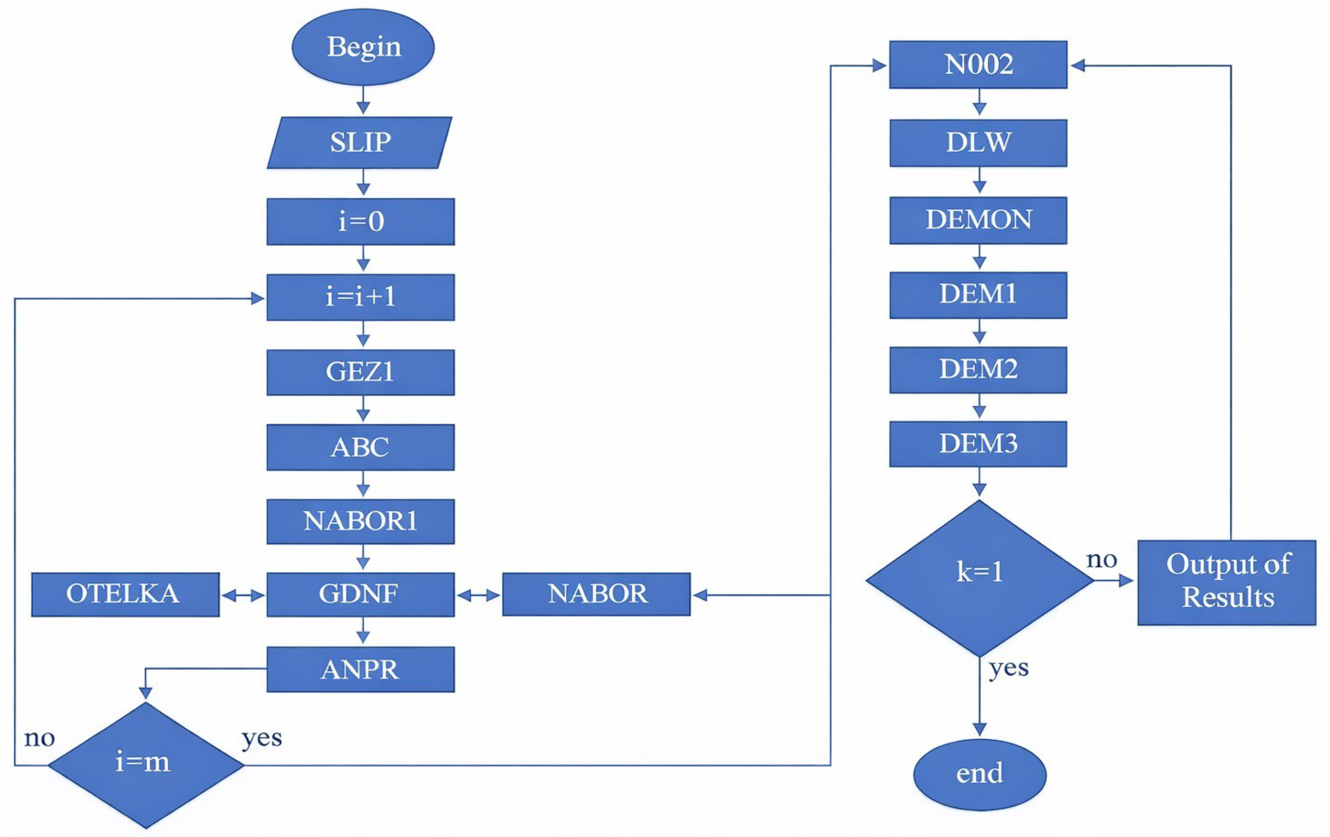
The RLSY program is designed to solve systems of second-degree nonlinear Boolean equations of a special class. It is implemented in the Basic programming language. The block diagram of RLSY is shown in Figure 1.
The program uses 14 procedures.
The SLIP procedure is a control procedure responsible for forming a dataset on a magnetic disk.
The GEZ1 (F, Z 1 , N 1 ) procedure is designed for grouping elements of statements in system R and encoding logical expressions (groupings) into the Z 1 array. Here,
F represents a Zhegalkin polynomial of a special type (a statement of system R);
Z 1 is an array of encoded logical expressions;
N 1 is the number of structural components (s.k.).
In the A B C ( L , A ) procedure,
L is the number of structural components in the A array;
A is an array of bit strings corresponding to structural components.
This procedure is used to transform structural components into bit-string arrays.
The procedure N A B O R ( B 2 , N , K ) forms the set of all sets V * = V 1 , V 2 , , V N , where V i * 0 , 1 , i = 1 , 2 , N such that V = i = 1 m V i = K , where
B 2 is the array of sets from the set F F K ;
N is the number of bits in vectors V * from F F K ;
K is the number of ones in the coordinates.
This procedure generates all possible combinations of sets (or vectors), where the sum of the elements in each vector equals K, corresponding to the number of ones in the vector.
The N A B O R 1 ( N 1 , B B , K 1 , T O ) procedure is designed to determine the elements V * from FF such that V * = V 1 , V 2 , , V n , where V 1 = V 2 = = V k = 1 ; V k + 1 = = V n = 0 , where
N 1 is the number of c.c.;
B B is a binary set;
K 1 is the number of one-bit positions;
T O is an auxiliary conditional parameter.
The O T E L K A ( H 1 , B T 1 , N , A A , C A ) procedure is used to perform transformations of the form: ¬ U 1   &   U 2   &     &   U m = ¬ U 1 ¬ U 2 ¬ U m ; U U 1 U m = U U 1 U U m , where U , , U m c . c .
Here, H 1 represents the number of c.c.; B T 1 is an array of bit strings for c.c.; N is the number of variables; A A and E A are arrays of bit strings corresponding to the DNF (disjunctive normal form) of the system’s logical statements.
The G D N F ( B 1 , B N 1 , N N , B 11 , C 11 , N , T 1 , K ) procedure transforms an array of bit strings of c.c. logical statements of the Zhegalkin polynomial into DNF:
B 1 —a bit string of c.c. statements of the Zhegalkin polynomial;
B N 1 —an array of elements;
N N —the number of c.c. of the Zhegalkin polynomial at input and the number of c.c. in DNF at output;
B 11 , C 11 —arrays of bit strings of c.c. in DNF;
N—the number of variables;
T 1 —an auxiliary conditional parameter;
K—the number of unit coordinates.
The A N P R ( N N , B 11 , C 11 , A N , Z ) procedure maps binary sets to an analytical representation and DNF for variable encoding:
N N —the number of elementary conjunctions in the DNF of system F F ;
B 11 , C 11 —arrays of binary sets representing the form;
A N —an elementary conjunction in analytical form;
N—the number of variables;
Z—an array of encoded functions.
Procedure N 002 ( N B , N , T , B ) generates index vectors of complex conjunctions (c.k.) during the multiplication of the system and, using subsequent procedures, constructs sets of solutions for system R:
N B —the number of equations in the system;
N—the number of variables;
T—an array containing the number of elementary conjunctions in the equations of system R;
B—an array of complex conjunctions in system R.
Procedure DLW (NB, L, B, SCH, K7, N)
This procedure performs the multiplication of complex conjunctions according to the index vector:
N B —an array defining the number of equations;
L—the size of array N B ;
B—an array of elementary conjunctions in the equations;
S C H —a conditional parameter;
K 7 —the size of array B;
N—the number of variables.
Procedure DEMON (N, N5, A, BB)
This procedure determines the structure of the resulting product of complex conjunctions:
B B —a vector corresponding to the Zhegalkin polynomial in the product;
A—a vector corresponding to the remaining part of the product B B ;
N 5 —the number of Zhegalkin polynomials in BB and the dimension of arrays A;
N—the number of variables.
Procedure DEM1 (N, N5, A, BB)
This procedure compares the part of the product represented in the form of the Zhegalkin polynomial with the remaining part and simplifies the product in case of intersections. The parameters N , N 5 , A , B B correspond to those in the DEMON procedure.
Procedure DEM2 (N, N5, A, BB)
This procedure forms sets of solutions corresponding to the remaining Zhegalkin polynomials. The parameters N , N 5 , A , B B correspond to those in the DEMON procedure.
Procedure DEM3 (N5, A, B, K1)
This procedure compares the sets of solutions obtained in DEM2 with the remaining part of the product and prints the resulting sets of solutions:
N 5 —the number of Zhegalkin polynomials in the product;
B—a vector corresponding to the Zhegalkin polynomial in the product;
A—a vector corresponding to the remaining part of the product;
K 1 —the dimension of vector A.

7. Instruction for the RLSY Program (Solution of Logical Systems of Equations)

The input data for the RLSY program (Resolution of Logical Systems of Equations) consists of the following:
N—number of variables;
M—number of equations;
F F i i = 1 , 2 , , M —formulas of the system of logical equations of a special second-degree class.
Since the solution set generated during the program execution can be very large, it is recommended to publish them gradually rather than storing them in a dedicated array or to stop the program periodically, printing partial results.
The input parameters, the system of second-order Boolean equations of a special class F F i i = 1 , 2 , , M and the sought solutions of the system are recorded as sets of size N, consisting of Z subsets. If a solution set is obtained, it corresponds to all possible solutions.
As a test example for the RLSY program (Solution of Logical Systems of Equations), we consider a system of equations where N = 10 and M = 20.
Test Example:
For simplicity and explanation, we take an analytical test example consisting of equations from a special class, divided into two groups, with 10 variables and α i = 1 i = 1 , 8 ¯ .
By grouping elements on the left-hand sides of the equations, we introduce new variables:
1. Now, to illustrate the effectiveness of this method, we will demonstrate how much the complexity of the given system has been reduced using simplicity indices.
Let us introduce the following notation:
[ U ¬ ( i = 1 m U i ) ] 0 . —the number of variable letters appearing in the notation of the left-hand sides of the equations.
[ U ¬ ( i = 1 m U i ) ] 0 . —the number of elementary conjunctions included in the equations.
α ˜ E n 2 —the complexity of the system is measured using L B and L K :
From this, we obtain m i = 1 U i ( α ˜ ) = 0 . The overall complexity difference between the systems is R = L R L R = 129 40 = 89 (See Table 5).
Thus, using this method, the complexity of the system is reduced by more than three times.
2. Using the formula α ˜ E n 2 , we transform the system R into its disjunctive normal form (DNF).
Naturally, the DNF may contain opposing complex conjunctions (i.e., terms that equal zero), which are excluded from the DNF.
Based on the program’s structure, the output can be a single solution, several solutions (k) as per the user’s preference, or all possible solutions.
In our approach, we determine multiple solutions for the given system. To achieve this, we select one complex conjunction from each equation and apply the method of linear equation systems.
Y 14 ¯ · Y 567 x 2 · Y 345 · Y 67910 ¯ x 3 · Y 456 · Y 78910 ¯ x 3 · Y 123 · Y 8910 ¯ x 4 · Y 234 · Y 6810 ¯ x 3 · Y 456 · Y 789 ¯ x 1 · Y 345 · Y 67910 ¯ x 2 Y 345 Y 67910 ¯ = 1
From this, it is easy to understand that x 1 = x 2 = x 3 = x 4 = 1 . They satisfy linear expressions at x 1 = x 2 = x 3 = x 4 = 1 ; Y 123 = Y 234 = Y 14 ¯ = 1 . Therefore, we will exclude them from the complex conjunction, leaving only one from Y 345 and one from x 5 = 1 and Y 67910 ¯ . From Y 345 , it follows that [ U ( α ˜ ) M ( α ˜ ) ] 1 . Consequently, from Y 456 we obtain x 6 = 1 , and further, we derive Y 567 x 7 = 1 . These are then excluded from the system of constraints (s.c.). Thus, we obtain
Y ¯ 67910 = Y ¯ 910 = 1 Y ¯ 78910 = Y 8910 = 1 Y ¯ 8910 = 1 Y ¯ 6810 = Y 810 = 1 Y ¯ 789 = Y 89 = 1 Y ¯ 67910 = Y ¯ 910 = 1
From this, it is evident that the first and last elements are identical and equivalent, so we remove one of them from the system. The second and third elements are incompatible (as they correspond to the third and fourth equations in the original system).
Thus, by eliminating each of them, we obtain the solution to the system for the special class.
A
Y ¯ 67910 = Y ¯ 910 = 1 Y ¯ 78910 = Y 8910 = 1 Y ¯ 6810 = Y 810 = 1 Y ¯ 789 = Y 89 = 1 x 9 x 10 1 = 1 x 8 x 9 x 10 = 1 x 8 x 10 = 1 x 8 x 9 = 1
The solution to this system is α ˜ E n 2 . Taking into account the previous variable roots, we obtain the general solution of the system without the fourth equation: 1 , 1 , 1 , 1 , 1 , 1 , 1 , 1 , 0 , 0 .
B
Thus, we obtain the general solution of the system without the third equation: 1 , 1 , 1 , 1 , 1 , 1 , 1 , 0 , 1 , 1 .

8. Conclusions

This article explores various transformations of logical formulas when transitioning from one basis to another in the process of solving systems of logical equations and determining their solution roots. The necessary criteria for formula transformations during basis transitions are established in the form of theorems, which describe the statements of Boolean equation systems. A solution is proposed for systems of second-degree nonlinear Boolean equations, which serve as a logical model for algebraic cryptanalysis. Test examples of logical formula transformations are provided. Additionally, a solution is presented for systems of second-degree nonlinear Boolean equations of a special class. The practical significance of the research results lies in the ability to solve systems of special second-degree nonlinear Boolean equations based on the grouping and minimization of logical statements in the class of disjunctive normal forms (DNFs), which serve as an algebraic model of S-boxes in symmetric encryption algorithms.

Author Contributions

Conceptualization, A.K. and I.S.; methodology, I.S.; software, A.B. (Alimdzhan Babadzhanov); validation, A.K., A.B. (Abdussattar Baizhumanov) and A.B. (Akbarjon Babadjanov); formal analysis, I.S.; investigation, A.B. (Alimdzhan Babadzhanov) and I.S.; resources, A.K., A.B. (Abdussattar Baizhumanov) and A.B. (Akbarjon Babadjanov); data curation, A.B. (Alimdzhan Babadzhanov); writing—original draft preparation, I.S.; writing—review and editing, A.B. (Alimdzhan Babadzhanov), A.B. (Abdussattar Baizhumanov) and A.B. (Akbarjon Babadjanov); visualization, A.B. (Akbarjon Babadjanov); supervision, I.S.; project administration, A.K. All authors have read and agreed to the published version of the manuscript.

Funding

This research received no external funding.

Data Availability Statement

No new data were created or analyzed in this study.

Acknowledgments

The author of the article, Islambek Saymanov, expresses gratitude to the participants of the project “AL-9424104925-R1”, implemented at the New Uzbekistan University, funded by the Agency for Innovative Development under the Ministry of Higher Education, Science and Innovation of the Republic of Uzbekistan, for their assistance in writing the article.

Conflicts of Interest

The authors declare no conflicts of interest.

References

  1. Chong, J.; Jiang, N.; Zhuo, Z.; Zhang, W. Boolean Functions with Two Distinct Nega-Hadamard Coefficients. IEICE Trans. Fundam. Electron. Commun. Comput. Sci. 2024, 107, 1603–1608. [Google Scholar] [CrossRef]
  2. Carlet, C. Boolean Functions for Cryptography and Coding Theory; Cambridge University Press: Cambridge, UK, 2020. [Google Scholar]
  3. Picek, S.; Carlet, C.; Guilley, S.; Miller, J.F.; Jakobovic, D. Evolutionary Algorithms for Boolean Functions in Diverse Domains of Cryptography. Evol. Comput. 2016, 24, 667–694. [Google Scholar] [CrossRef]
  4. Garcia, F.; Simmons, H.; Kumar, S. Classification of Boolean Functions. Discret. Appl. Math. 2022, 290, 9–23. [Google Scholar]
  5. Bushnell, M.L.; Agrawal, V.D. Essentials of Electronic Testing for Digital, Memory and Mixed-Signal VLSI Circuits; Kluwer Academic Publishers: Boston, MA, USA, 2000. [Google Scholar]
  6. O’Donnell, R. Analysis of Boolean Functions; Cambridge University Press: New York, NY, USA, 2014. [Google Scholar] [CrossRef]
  7. Lee, S.-Y.; Riener, H.; Mishchenko, A.; Brayton, R.K.; De Micheli, G. A Simulation-Guided Paradigm for Logic Synthesis and Verification. IEEE Trans. Comput.-Aided Des. Integr. Circuits Syst. 2022, 41, 2573–2586. [Google Scholar] [CrossRef]
  8. Wang, C.; Agarwal, R.P.; Regan, D.O.; Sakthivel, R. Theory of Translation Closedness for Time Scales; Springer Nature: New York, NY, USA, 2020. [Google Scholar] [CrossRef]
  9. Ahmed, M.; Baker, T.; Patel, S. On the Cryptographic Properties of Boolean Functions. J. Cryptogr. Eng. 2022, 12, 231–245. [Google Scholar]
  10. Muhiddinov, M.; Ochilov, N.; Umurkulov, B.; Kholnazarov, U.; Sapaev, I.; Bazarova, N.; Kholova, M.; Aripova, G. Privacy-Aware Information Security for E-Learning Platforms in History Using Attribute-Based Encryption Algorithm. J. Internet Serv. Inf. Secur. 2025, 15, 305–-315. [Google Scholar] [CrossRef]
  11. Xia, B.; Mantegh, I.; Xie, W.-F. Hybrid Framework for UAV Motion Planning and Obstacle Avoidance: Integrating Deep Reinforcement Learning with Fuzzy Logic. In Proceedings of the 2024 10th International Conference on Control, Decision and Information Technologies (CoDIT), Valletta, Malta, 1–4 July 2024; Volume 9, pp. 2662–2669. [Google Scholar] [CrossRef]
  12. Bakhronova, D.; Narziyeva, M.; Yuldosheva, N.; Zayniyeva, U.; Yusupov, J.; Uralov, B.; Sapaev, I.; Khikmatov, N. Intelligent Information Security System for Language and History Education Using Machine Learning-based Intrusion Detection Algorithm. J. Internet Serv. Inf. Secur. 2025, 15, 520–529. [Google Scholar] [CrossRef]
  13. Kabulov, A.; Saymanov, I.; Yarashov, I.; Muxammadiev, F. Algorithmic method of security of the Internet of Things based on steganographic coding. In Proceedings of the 2021 IEEE International IOT, Electronics and Mechatronics Conference (IEMTRONICS), Toronto, ON, Canada, 21–24 April 2021; pp. 1–5. [Google Scholar] [CrossRef]
  14. Cusick, T.W.; Stănică, P. Cryptographic Boolean Functions and Applications; Academic Press: San Diego, CA, USA, 2017. [Google Scholar]
  15. Srinivasan, C.; Lakshmy, K.V.; Sethumadhavan, M. Complexity measures of cryptographically secure boolean functions. In Cyber Security Cyber Crime and Cyber Forensics Applications and Perspectives; IGI Global: Hershey, PA, USA, 2011; pp. 220–230. [Google Scholar] [CrossRef]
  16. Rosen, K.H. Discrete Mathematics and Its Applications, 8th ed; McGraw-Hill: New York, NY, USA, 2019; p. 1120. [Google Scholar]
  17. Zheng, J. Security analysis of Boolean algebra based on Zhang-Wang digital signature scheme. AIP Conf. Proc. 2014, 1618, 507–509. [Google Scholar] [CrossRef]
  18. Kim, J.; Nguyen, F.; Lee, S. Boolean Functions in Cryptography. IEEE Trans. Inf. Theory 2024, 70, 310–325. [Google Scholar]
  19. Green, R.; Ahmed, L.; Qureshi, N. Circuit Realizations of Boolean Functions. J. Log. Comput. 2021, 31, 222–236. [Google Scholar]
  20. Jackson, T.; Velasquez, M.; Dutta, R. Spectral Properties of Boolean Functions. Comput. Complex. 2022, 29, 1065–1079. [Google Scholar]
  21. Kim, D.; Nair, V.; Zhang, X. Boolean Functions in Quantum Computing. Quantum Comput. Quantum Inf. 2022, 33, 12–29. [Google Scholar]
  22. Jukna, S. Boolean Function Complexity: Advances and Frontiers; Springer: Berlin, Germany, 2012. [Google Scholar] [CrossRef]
  23. Ballani, F. The surface pair correlation function for stationary Boolean models. Adv. Appl. Probab. 2007, 39, 1–15. [Google Scholar] [CrossRef][Green Version]
  24. Wegener, I. The Complexity of Boolean Functions; John Wiley & Sons: Chichester, UK, 1987. [Google Scholar]
  25. López-López, I.; Sosa-Gómez, G.; Segura, C.; Oliva, D.; Rojas, O. Metaheuristics in the Optimization of Cryptographic Boolean Functions. Entropy 2020, 22, 1052. [Google Scholar] [CrossRef]
  26. Bonich, T.A.; Panferov, M.A.; Tokareva, N.N. On the number of -suitable Boolean functions in constructions of filter and combining models of stream ciphers. Prikl. Diskretn. Mat. 2023, 62, 1211–1216. [Google Scholar] [CrossRef]
  27. Sun, Q.; Wei, S.; Saymanov, I.; Lu, Y.; Deng, W.; Lou, J. A Mechanical–Electrical Damage Model for Performance Analysis of Crack-based Strain Sensor. Int. J. Appl. Mech. Source Preview 2025, 18, 2550124. [Google Scholar] [CrossRef]
  28. Sun, Z.; Ambrosi, E.; Bricalli, A.; Ielmini, D. Logic Computing with Stateful Neural Networks of Resistive Switches. Adv. Mater. 2018, 30, 1802554. [Google Scholar] [CrossRef]
  29. Stallings, W. Cryptography and Network Security: Principles and Practice, 7th ed.; Pearson Prentice Hall: Boston, MA, USA, 2017. [Google Scholar]
  30. Mesnager, S. Bent Functions: Fundamentals and Results; Springer: Cham, Switzerland, 2016. [Google Scholar] [CrossRef]
  31. Brayton, R.K.; Hachtel, G.D.; McMullen, C.T.; Sangiovanni-Vincentelli, A.L. Logic Minimization Algorithms for VLSI Synthesis; Kluwer Academic Publishers: Boston, MA, USA, 1984. [Google Scholar] [CrossRef]
  32. Yang, Y.; Zhang, L.; An, L. Fixed-Time Adaptive Fault-Tolerant Control for Uncertain Nonlinear Systems with Actuator Faults. Appl. Math. Comput. 2025, 516, 129867. [Google Scholar] [CrossRef]
  33. Kuzmin, A.S.; Markov, V.T.; Nechaev, A.A.; Neljubin, A.S. A Generalization of the Binary Preparata Code. Discret. Appl. Math. 2005, 154, 337–345. [Google Scholar] [CrossRef][Green Version]
  34. Hiep, X.H.; Bao, H.L.; Hung, V.C.L.; Tam, T.L.; Nghia, D.-T. Design of an IoT ultrasonic-vision based system for automatic fruit sorting utilizing size and color. Internet Things 2024, 25, 101017. [Google Scholar] [CrossRef]
  35. Tran, T.C.T.; Phan, L.P.; Huynh, H.X. Approach of Item-Based Collaborative Filtering Recommendation Using Energy Distance. J. Adv. Inf. Technol. 2024, 15, 10–16. [Google Scholar] [CrossRef]
  36. Shukla, S.; Hussain, S.; Irshad, R.R.; Alattab, A.A.; Thakur, S.; Breslin, J.G.; Hassan, M.F.; Abimannan, S.; Husain, S.; Jameel, S.M. Network analysis in a peer-to-peer energy trading model using blockchain and machine learning. Comput. Stand. Interfaces 2024, 88, 103799. [Google Scholar] [CrossRef]
  37. Chang, Y.-S.; Huang, S.-T.; Haobijam, B.; Abimannan, S.; Kushida, T. Marine ecological information prediction by using adjacent location spatiotemporal deep learning model with ensemble learning techniques. Ecol. Inform. 2025, 85, 102964. [Google Scholar] [CrossRef]
  38. Gotarane, V.; Abimannan, S.; Hussain, S.; Irshad, R.R. A Hybrid Framework Leveraging Whale Optimization and Deep Learning With Trust-Index for Attack Identification in IoT Networks. IEEE Access 2024, 12, 36296–36310. [Google Scholar] [CrossRef]
  39. She, Y.; Hong, Y.; Shen, S.; Yang, B.; Zhang, L.; Wang, J. Consistency regularization for few shot multivariate time series forecasting. Sci. Rep. 2025, 15, 14195. [Google Scholar] [CrossRef]
  40. Makhmudov, F.; Privalov, A.; Egorenkov, S.; Pryadkin, A.; Kutlimuratov, A.; Bekbaev, G.; Cho, Y.I. Analytical Approach to UAV Cargo Delivery Processes Under Malicious Interference Conditions. Mathematics 2025, 13, 2008. [Google Scholar] [CrossRef]
  41. Kabulov, A.; Baizhumanov, A.; Saymanov, I. Synthesis of Optimal Correction Functions in the Class of Disjunctive Normal Forms. Mathematics 2024, 12, 2120. [Google Scholar] [CrossRef]
  42. Saymanov, I. Logical automatic implementation of steganographic coding algorithms. J. Math. Mech. Comput. Sci. 2024, 121, 122–131. [Google Scholar] [CrossRef]
  43. Kabulov, A.; Normatov, I.; Saymanov, I.; Baizhumanov, A. On the Completeness of Classes of Correcting Functions of Heuristic Algorithms. Azerbaijan J. Math. 2025, 15, 51–64. [Google Scholar] [CrossRef]
  44. GOST R 34.12-2015; Information Technology. Cryptographic Data Security. Block Ciphers. Technical Committee for Standardization “Cryptography and Security Mechanisms” (TC 26): Moscow, Russia, 2015.
Figure 1. Algorithm for solving logical equation systems.
Mathematics 14 00594 g001
Table 1. Formula representation in the reduced basis.
X X 1 X 2 X 3 X 4 X 5
R
11*10*1
2*0101
3**0*0
40*0*0
1 *—accepts an arbitrary value (0 or 1) and does not affect the remaining values, which makes no difference.
Table 2. The result of the obtained formula.
X X 1 X 2 X 3 X 4 X 5
U i
1* 111**
2**11*
3**1*0
401**1
50**11
60*0**
1 *—accepts an arbitrary value (0 or 1) and does not affect the remaining values, which makes no difference.
Table 3. The solution of the equation using Formula (6).
Number of Solutions
F 5 = 1 ; F 5 = 1 ; F 5 = 1 ;
F 4 = 0 ; F 4 = 1 ; F 4 = 1 ;
F 1 , F 2 , F 3 -optional F 3 = 0 , F 1 , F 2 -optional F 3 = 1 , F 2 = 1 , F 3 = 0
841
Table 4. The solution of the equation using the Formula (7).
Number of Solutions
x 4 = 1 ; x 4 = 1
x 5 = 0 x 5 = 1
x 1 , x 2 , x 3 -optional x 3 = 1 ; ( x 1 , x 2 ) = 0
83
Table 5. General difference in system complexity.
No. U ( α ˜ ) = 1 ¬ ( i = 1 m U i ( α ˜ ) ) = 1 U ( α ˜ ) = 1 U ( x ˜ , y ( x ˜ ) ) = 1 U 1 ( x ˜ , y ( x ˜ ) ) = 0 U m ( x ˜ ,   y ( x ˜ ) ) = 0          α ˜ U ( α ˜ ) = 1
i = 1 117183        25
i = 2 107173        25
i = 3 107173        25
i = 4 96153        25
i = 5 96153        25
i = 6 96153        25
i = 7 107173        25
i = 8 96153        25
Total775212924        1640
Disclaimer/Publisher’s Note: The statements, opinions and data contained in all publications are solely those of the individual author(s) and contributor(s) and not of MDPI and/or the editor(s). MDPI and/or the editor(s) disclaim responsibility for any injury to people or property resulting from any ideas, methods, instructions or products referred to in the content.