A Novel Twin-Bounded Support Vector Machine with Smooth Generalized Pinball Loss

Abstract

We present a one-parameter family of smooth generalized pinball loss functions to overcome the challenges of non-differentiability, noise sensitivity, and resampling instability inherent in traditional loss functions such as hinge loss. These functions make the objective function in the formulation of the support vector machine (SVM) model twice continuously differentiable and improve model performance by reducing noise sensitivity and preserving the sparsity of the solution. Similarly, a novel twin-bounded support vector machine (TBSVM) model with a smooth generalized pinball loss function is obtained. Furthermore, we compare the performance of the TBSVM with the novel type of smooth loss function against other contemporary approaches, offering a comprehensive assessment of its strengths and limitations by conducting an evaluation with UCI datasets. The experimental results show that the proposed model has the best performance in the TBSVM with RBFSampler. Additionally, we prove that the generalized pinball loss function can be approximated by a novel smooth generalized pinball loss function in the uniform norm with arbitrary precision. We further show that the solutions of the proposed SVM and TBSVM models are unique and that they converge to the solutions of the models with non-smooth generalized pinball loss as the parameter approaches zero.

1. Introduction

The support vector machine (SVM), as introduced by Vapnik and Cortes [1], is a machine learning technique founded on the principles of the Vapnik–Chervonenkis (VC) dimension and structural risk minimization theory within the realm of statistical learning. It is a powerful and widely used supervised machine learning algorithm that is primarily employed for classification and regression tasks, such as text categorization [2], or scene classification [3], to name just a few examples. When applied to classification, this approach employs a strategy of maximizing the distances between two distinct data classes from a separating hyperplane, ensuring the correct classification of the two training datasets with a high level of confidence. Through the introduction of “slack variables” and the “kernel trick”, SVMs are particularly suited for their ability to effectively handle high-dimensional data and complex, non-linear decision boundaries.

The twin support vector machine (TWSVM), an innovative extension of the traditional SVM, has garnered considerable attention for its potential to address complex data distributions. Khemchandani and Chandra [4] proposed the TWSVM, which consists of two non-parallel hyperplanes, each positioned in close proximity to one of the two classes while maintaining a minimum separation distance from the other class. The TWSVM reduces the algorithmic complexity to just a quarter of that of the standard SVM, resulting in a significant reduction of computational time. Shao and his research team [5] modified the TWSVM to the twin-bounded support vector machine (TBSVM), aiming to minimize structural risk and leading to improved general performance.

Creating the hyperplanes in any of the support vector machine models involves solving a constrained convex minimization problem. The most common solution technique is to formulate the dual optimization problem and solve it using the method of Lagrange multipliers. More recently, techniques for solving the primal problem directly have become popular. These methods use a “loss function” to reformulate the problem as an unconstrained optimization problem. Common loss functions include the hinge loss, the pinball loss [6], and the generalized pinball loss functions [7], listed in order of complexity. Because these loss functions are not differentiable, efficient numerical methods such as gradient descent or Newton methods cannot be applied, or cannot be applied based on a solid theoretical foundation. A theoretical analysis generally requires that the objective functions be of $C^2$ type, that is, twice continuously differentiable.

In 2023, Makmuang, Ratiphaphongthon, and Wangkeeree introduced a $C^1$-smooth approximation to the generalized pinball loss function within the standard SVM framework [8]. The results demonstrate that, on average, the proposed method exhibits superior performance compared to the baseline models. Similarly, Kai and Zhen [9] introduced a smooth approximation to the pinball loss function in the twin-bounded support vector machine model to mitigate the noise sensitivity and resampling instability associated with the hinge loss function.

A variety of further loss functions have been proposed in the literature. In [10], a piecewise-quadratic loss is introduced that smooths the pinball loss and belongs to the class of $C^1$-functions. In [11], a truncated $epsilon$-insensitive pinball loss is investigated, which is only piecewise $C^1$. In [12], the pinball loss is modified by an S-curve to obtain a family of $C^1$ loss functions depending on three parameters. In [13], a quartic truncated pinball loss is introduced, which is $C^1$ and bounded; hence, it is non-convex. Furthermore, in [14], a rescaled huberized pinball loss is discussed, which again is $C^1$, bounded, and non-convex. Finally, recent studies [15] have explored interesting hybrid data–physics loss formulations, which incorporate physical constraints or domain knowledge into the training process. While such approaches may offer improved interpretability, they are tailored to specific applications and require knowledge of the physical setting. Thus, there is a scarcity of $C^2$-smooth convex loss functions that approximate the pinball loss and can be applied to a variety of data.

The main contributions of this work can be summarized as follows. First, we propose a novel one-parameter family of $C^2$-smooth loss functions, rendering the objective function in the unconstrained formulation of the SVM $C^2$-smooth as well. We further show that the novel smooth functions can approximate the non-smooth generalized pinball loss function with arbitrary precision in the uniform norm. Second, the proposed smooth loss is incorporated into the twin-bounded support vector machine framework, for which we rigorously prove the uniqueness of solutions and their convergence to the solutions obtained from the non-smooth generalized pinball loss as the smoothing parameter approaches zero. Third, unlike existing smooth pinball or generalized pinball loss formulations, our work provides a complete theoretical foundation for both SVM and TBSVM models, linking smooth loss approximation, optimization stability, and solution behavior. Finally, numerical experiments on benchmark datasets demonstrate that the proposed approach achieves competitive accuracy with stable training behavior.

By comparing the TBSVM equipped with this novel loss function against other contemporary approaches, this study aims to provide a comprehensive perspective on the strengths and limitations of this methodology. It primarily concentrates on conducting an extensive comparative analysis to investigate the impact of various loss functions and their generalizations on model performance. Additionally, it proves that the generalized pinball loss function can be arbitrarily approximated by one of the smooth loss functions in the uniform norm.

The remainder of this paper is organized as follows. Section 2 reviews background material on SVMs, TWSVMs, TBSVMs, and loss functions. Section 3 introduces the proposed smooth generalized pinball loss and presents theoretical analysis. Section 4 reports on numerical experiments, and Section 5 concludes the paper.

2. Background and Literature Review

This section introduces the fundamental mathematical concepts in machine learning as they pertain to the support vector machine models used in this work.

2.1. The Support Vector Machine

Let $X=\{(\overrightarrow{x_i},y_i):i=1,2,\dots ,m\}$ be a training data set, where $\overrightarrow{x_i}\in {\mathbf{R}}^n$ and $y_i\in \{+1,-1\}$. Here, m denotes the number of data samples, n the number of features, and $y_i$ the class to which a data sample belongs. A linear support vector machine (SVM) finds the optimal hyperplane

$$f\left(\overrightarrow{x}\right)={\overrightarrow{w}}^T\overrightarrow{x}+b=0,$$

which separates the data into two classes and has the largest distance from each of the two classes; this distance is called the margin. The vector $\overrightarrow{w}$ is normal to the hyperplane and determines its direction in n-space, while the offset b reflects its distance from the origin. The decision function of an SVM, which determines the class a data sample $\overrightarrow{x}$ belongs to, is obtained from the sign function (sgn) by

$$\mathrm{class}\left(\overrightarrow{x}\right)=\mathrm{sgn}({\overrightarrow{w}}^T\overrightarrow{x}+b).$$

(1)

In practice, it may not be possible to properly separate the two data classes by means of a single hyperplane. One thus allows for misclassification of some of the training data samples, and can find the hyperplane by solving an unconstrained optimization problem:

$$\underset{\overrightarrow{w},b}{min}{\displaystyle \frac{1}{2}}\left(\parallel \overrightarrow{w}{\parallel }^2+b^2\right)+{\displaystyle \frac{C}{m}}\sum _{i=1}^m{L}_{\mathbf{hinge}}\left(1-y_i({\overrightarrow{w}}^T\overrightarrow{x_i}+b)\right),$$

(2)

where the function $L_{\mathbf{hinge}}$ is the hinge loss function defined on the real line by

$$L_{\mathbf{hinge}}\left(u\right)=max\{0,u\}=\left\{\begin{array}{cc}u,\hfill & u\ge 0,\hfill \\ 0,\hfill & u<0.\hfill \end{array}\right.$$

(3)

The term on the right of (2) reflects the amount of misclassification, and the parameter $C>0$ manages the equilibrium between maximizing the margin and minimizing classification errors.

2.2. The Twin Support Vector Machine

Consider a binary classification dataset X, which contains $m_1$ positive (class $+1$) and $m_2$ negative (class $-1$) samples, respectively, with $m_1+m_2=m$. In a twin support vector machine (TWSVM), two non-parallel hyperplanes are located in a manner where each hyperplane is nearer to one of the two classes and maintains a minimum margin of at least one from the other. The two nonparallel classification hyperplanes take the following form:

$$f_1\left(\overrightarrow{x}\right)={\overrightarrow{w_1}}^T\overrightarrow{x}+b_1=0\mathrm{and}{f}_2\left(\overrightarrow{x}\right)={\overrightarrow{w_2}}^T\overrightarrow{x}+b_2=0,$$

and need to separate the samples correctly. Thus, the TWSVM is determined by the following two unconstrained optimization problems:

$$\underset{\overrightarrow{w_1},b_1}{min}{\displaystyle \frac{1}{2}}\sum _{i=1}^{m_1}{({\overrightarrow{w_1}}^T{\overrightarrow{x_i}}^{\left(1\right)}+b_1)}^2+{\displaystyle \frac{c_1}{m_2}}\sum _{i=1}^{m_2}{L}_{\mathbf{hinge}}\left(1+({\overrightarrow{w_1}}^T{\overrightarrow{x_i}}^{\left(2\right)}+b_1)\right),$$

(4)

and

$$\underset{\overrightarrow{w_2},b_2}{min}{\displaystyle \frac{1}{2}}\sum _{i=1}^{m_2}{({\overrightarrow{w_2}}^T{\overrightarrow{x_i}}^{\left(2\right)}+b_2)}^2+{\displaystyle \frac{c_2}{m_1}}\sum _{i=1}^{m_1}{L}_{\mathbf{hinge}}\left(1-({\overrightarrow{w_2}}^T{\overrightarrow{x_i}}^{\left(1\right)}+b_2)\right),$$

(5)

where ${\overrightarrow{x_i}}^{\left(1\right)}$$(i=1\dots m_1)$ and ${\overrightarrow{x_i}}^{\left(2\right)}$$(i=1\dots m_2)$ denote the data samples in the positive and negative class, respectively. The decision function of the TWSVM is

$${\displaystyle \mathrm{class}\left(\overrightarrow{x}\right)=\mathrm{sign}\left(\frac{{\overrightarrow{w_1}}^T\overrightarrow{x}+b_1}{\parallel \overrightarrow{w_1}\parallel }+\frac{{\overrightarrow{w_2}}^T\overrightarrow{x}+b_2}{\parallel \overrightarrow{w_2}\parallel }\right).}$$

(6)

2.3. The Twin-Bounded Support Vector Machine

The objective function of the TWSVM saw the integration of a regularization term by Shao and his research team in 2011 [5], resulting in the introduction of a novel machine learning model called the twin-bounded support vector machine (TBSVM). It is formulated as

$$\underset{\overrightarrow{w_1},b_1}{min}{\displaystyle \frac{1}{2}}\sum _{i=1}^{m_1}{({\overrightarrow{w_1}}^T{\overrightarrow{x_i}}^{\left(1\right)}+b_1)}^2+{\displaystyle \frac{c_3}{2}}(\parallel \overrightarrow{w_1}{\parallel }^2+b_1^2)+{\displaystyle \frac{c_1}{m_2}}\sum _{i=1}^{m_2}{L}_{\mathbf{hinge}}\left(1+({\overrightarrow{w_1}}^T{\overrightarrow{x_i}}^{\left(2\right)}+b_1)\right),$$

(7)

and

$$\underset{\overrightarrow{w_2},b_2}{min}{\displaystyle \frac{1}{2}}\sum _{i=1}^{m_2}{({\overrightarrow{w_2}}^T{\overrightarrow{x_i}}^{\left(2\right)}+b_2)}^2+{\displaystyle \frac{c_4}{2}}(\parallel \overrightarrow{w_2}{\parallel }^2+b_2^2)+{\displaystyle \frac{c_2}{m_1}}\sum _{i=1}^{m_1}{L}_{\mathbf{hinge}}\left(1-({\overrightarrow{w_2}}^T{\overrightarrow{x_i}}^{\left(1\right)}+b_2)\right).$$

(8)

A survey on various twin support machine variants can be found in [16].

2.4. Loss Functions

The hinge loss function $L_{\mathbf{hinge}}\left(u\right)$ is unstable for resampling and sensitive to noise. To resolve this problem, in 2013, Huang, Shi, and Suykens [6] modified it to the pinball loss function in the SVM classifier, and demonstrated its effectiveness in mitigating noise sensitivity through experiments. The pinball loss function is defined as follows

$$L_{\tau }\left(u\right)=\left\{\begin{array}{cc}u,\hfill & u\ge 0,\hfill \\ -\tau u,\hfill & u<0,\hfill \end{array}\right.$$

(9)

where $\tau$ is a non-negative real parameter. However, the pinball loss function still shows some noise sensitivity. Thus, the $ϵ$-insensitive pinball loss function was created, defined as

$$L_{\tau }^{ϵ}\left(u\right)=\left\{\begin{array}{cc}u-ϵ,\hfill & u>ϵ,\hfill \\ 0,\hfill & -{\displaystyle \frac{ϵ}{\tau }}\le u\le ϵ,\hfill \\ -\tau (u+{\displaystyle \frac{ϵ}{\tau }}),\hfill & u<-{\displaystyle \frac{ϵ}{\tau }},\hfill \end{array}\right.$$

(10)

where $\tau ,ϵ$ are non-negative real values. Recently, Rastogi, Pal, and Chandra [7] introduced a novel loss function generalizing the $ϵ$-insensitive pinball loss by introducing one more parameter. This is generalized pinball loss; it is defined by

$$L_{{\tau }_1,{\tau }_2}^{{ϵ}_1,{ϵ}_2}\left(u\right)=\left\{\begin{array}{cc}{\tau }_1(u-{\displaystyle \frac{{ϵ}_1}{{\tau }_1}}),\hfill & u>{\displaystyle \frac{{ϵ}_1}{{\tau }_1}},\hfill \\ 0,\hfill & -{\displaystyle \frac{{ϵ}_2}{{\tau }_2}}\le u\le {\displaystyle \frac{{ϵ}_1}{{\tau }_1}},\hfill \\ -{\tau }_2(u+{\displaystyle \frac{{ϵ}_2}{{\tau }_2}}),\hfill & u<-{\displaystyle \frac{{ϵ}_2}{{\tau }_2}},\hfill \end{array}\right.$$

(11)

where ${\tau }_1,{\tau }_2,{ϵ}_1,{ϵ}_2$ are non-negative parameters.

Makmuang, Ratiphaphongthon, and Wangkeeree [8] introduced a new $C^1$-smooth loss function that approximates the generalized pinball loss function for use in the SVM, which is given by

$$Q_{{\tau }_1,{\tau }_2}^{{ϵ}_1,{ϵ}_2}(u,\mu )=\left\{\begin{array}{cc}{\tau }_1(u-{\displaystyle \frac{{ϵ}_1}{{\tau }_1}})-{\displaystyle \frac{{\tau }_1^2}{2}}\mu ,\hfill & {\displaystyle \frac{{ϵ}_1}{{\tau }_1}}+{\tau }_1\mu \le u,\hfill \\ {\displaystyle \frac{1}{2\mu }}{(u-{\displaystyle \frac{{ϵ}_1}{{\tau }_1}})}^2,\hfill & {\displaystyle \frac{{ϵ}_1}{{\tau }_1}}\le u\le {\displaystyle \frac{{ϵ}_1}{{\tau }_1}}+{\tau }_1\mu ,\hfill \\ 0,\hfill & -{\displaystyle \frac{{ϵ}_2}{{\tau }_2}}\le u\le {\displaystyle \frac{{ϵ}_1}{{\tau }_1}},\hfill \\ {\displaystyle \frac{1}{2\mu }}{(u+{\displaystyle \frac{{ϵ}_2}{{\tau }_2}})}^2,\hfill & -{\displaystyle \frac{{ϵ}_2}{{\tau }_2}}-{\tau }_2\mu \le u\le -{\displaystyle \frac{{ϵ}_2}{{\tau }_2}},\hfill \\ -{\tau }_2(u+{\displaystyle \frac{{ϵ}_2}{{\tau }_2}})-{\displaystyle \frac{{\tau }_2^2}{2}}\mu ,\hfill & u\le -{\displaystyle \frac{{ϵ}_2}{{\tau }_2}}-{\tau }_2\mu ,\hfill \end{array}\right.$$

(12)

where ${\tau }_1,{\tau }_2,{ϵ}_1,{ϵ}_2$ are non-negative real values, $u\in \mathbb{R}$, and $\mu \in {\mathbb{R}}_{+}$ is a parameter of how close $Q_{{\tau }_1,{\tau }_2}^{{ϵ}_1,{ϵ}_2}(·,\mu )$ approximates $L_{{\tau }_1,{\tau }_2}^{{ϵ}_1,{ϵ}_2}(·)$.

Alternatively, Kai and Zhen [9] proposed an infinitely differentiable approximation of the pinball loss function within the twin-bounded support vector machine model to mitigate the noise sensitivity and resampling instability inherent in the pinball loss function. Their smooth approximation of the pinball loss function is defined as

$${\varphi }_{\tau }(u,ϵ)={\displaystyle \frac{u+\sqrt{u^2+4{ϵ}^2}}{2}}+{\displaystyle \frac{-\tau u+\sqrt{{\tau }^2{u}^2+4{ϵ}^2}}{2}},$$

(13)

where $\tau ,ϵ$ are non-negative real parameter values.

3. Proposed Work

This section proposes a novel one-parameter family of $C^2$ loss functions, presents the proof of uniform convergence to the generalized pinball loss function with decreasing parameter, and develops and analyzes an SVM model and a TBSVM model incorporating the novel loss.

3.1. The Proposed Smooth Loss Function

To smooth the generalized pinball loss $L_{{\tau }_1,{\tau }_2}^{{ϵ}_1,{ϵ}_2}\left(u\right)$, we define functions $P_{{\tau }_1,{\tau }_2}^{{ϵ}_1,{ϵ}_2}(u,\mu )$: $\mathbb{R}\times {\mathbb{R}}^{+}\to {\mathbb{R}}^{+}$, which depend on the real variable u and are parameterized by an approximation parameter $\mu >0$, by

$$P_{{\tau }_1,{\tau }_2}^{{ϵ}_1,{ϵ}_2}(u,\mu )=\left\{\begin{array}{cc}{\tau }_1(u-{\displaystyle \frac{{ϵ}_1}{{\tau }_1}})-{\displaystyle \frac{5}{8}}{\tau }_1^2\mu ,\hfill & {\displaystyle \frac{{ϵ}_1}{{\tau }_1}}+{\tau }_1\mu <u,\hfill \\ {\displaystyle \frac{5}{8{\tau }_1^2{\mu }^3}}{(u-{\displaystyle \frac{{ϵ}_1}{{\tau }_1}})}^4-{\displaystyle \frac{1}{4{\tau }_1^4{\mu }^5}}{(u-{\displaystyle \frac{{ϵ}_1}{{\tau }_1}})}^6,\hfill & {\displaystyle \frac{{ϵ}_1}{{\tau }_1}}<u\le {\displaystyle \frac{{ϵ}_1}{{\tau }_1}}+{\tau }_1\mu ,\hfill \\ 0,\hfill & -{\displaystyle \frac{{ϵ}_2}{{\tau }_2}}\le u\le {\displaystyle \frac{{ϵ}_1}{{\tau }_1}},\hfill \\ {\displaystyle \frac{5}{8{\tau }_2^2{\mu }^3}}{(u+{\displaystyle \frac{{ϵ}_2}{{\tau }_2}})}^4-{\displaystyle \frac{1}{4{\tau }_2^4{\mu }^5}}{(u+{\displaystyle \frac{{ϵ}_2}{{\tau }_2}})}^6,\hfill & -{\displaystyle \frac{{ϵ}_2}{{\tau }_2}}-{\tau }_2\mu \le u<-{\displaystyle \frac{{ϵ}_2}{{\tau }_2}},\hfill \\ -{\tau }_2(u+{\displaystyle \frac{{ϵ}_2}{{\tau }_2}})-{\displaystyle \frac{5}{8}}{\tau }_2^2\mu ,\hfill & u<-{\displaystyle \frac{{ϵ}_2}{{\tau }_2}}-{\tau }_2\mu .\hfill \end{array}\right.$$

(14)

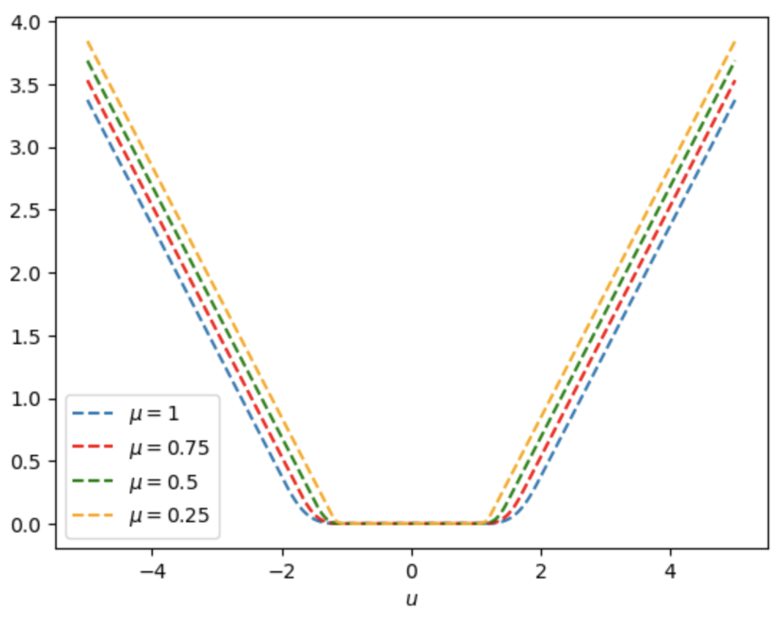
where the parameters ${\tau }_1,{\tau }_2,{ϵ}_1,{ϵ}_2$ take non-negative real values. Note that when $\mu =0$, we recover the generalized pinball loss $L_{{\tau }_1,{\tau }_2}^{{ϵ}_1,{ϵ}_2}\left(u\right)$. Figure 1 displays the graphic representation of $P_{{\tau }_1,{\tau }_2}^{{ϵ}_1,{ϵ}_2}(u,\mu )$ for various values of the parameter $\mu$, with ${\tau }_1,{\tau }_2,{ϵ}_1,{ϵ}_2$ fixed (${\tau }_1,{\tau }_2,{ϵ}_1,{ϵ}_2=1$).

It is easy to verify that the $P_{{\tau }_1,{\tau }_2}^{{ϵ}_1,{ϵ}_2}(u,\mu )$ are $C^2$-functions and belong to a category of smoothing functions for $L_{{\tau }_1,{\tau }_2}^{{ϵ}_1,{ϵ}_2}\left(u\right).$ Figure 1 hints that the mapping $P_{{\tau }_1,{\tau }_2}^{{ϵ}_1,{ϵ}_2}(u,\mu )$ converges to $L_{{\tau }_1,{\tau }_2}^{{ϵ}_1,{ϵ}_2}\left(u\right)$ as $\mu \to 0^{+}$, which we will prove.

In the support vector machine models described below, the parameters ${\tau }_1$ and ${\tau }_2$ control the asymmetric penalties assigned to positive and negative misclassification errors, respectively, while ${\epsilon }_1$ and ${\epsilon }_2$ determine the width of the insensitivity region and thus tolerance to noise. The smoothing parameter $\mu$ governs the trade-off between approximation accuracy and the numerical smoothness: smaller values of $\mu$ yield a closer approximation to the original generalized pinball loss, whereas larger values improve numerical stability during optimization.

In the following proofs, we will use the symbols $L\left(u\right)$ and $P(u,\mu )$ in place of $L_{{\tau }_1,{\tau }_2}^{{ϵ}_1,{ϵ}_2}\left(u\right)$ and $P_{{\tau }_1,{\tau }_2}^{{ϵ}_1,{ϵ}_2}(u,\mu )$, respectively, since the parameters ${\tau }_1,{\tau }_2,{ϵ}_1,{ϵ}_2$ remain fixed.

The next theorem shows that our proposed smooth loss functions indeed approach the generalized pinball loss uniformly as the parameter $\mu$ tends to zero.

Theorem 1.

Let $L\left(u\right)$ and $P(u,\mu )$ be defined as in (11) and (14), respectively. Then

(i)  

for all $u\in R$, ${\displaystyle 0\le L\left(u\right)-P(u,\mu )\le \frac{5}{8}{\tau }_0^2\mu }$, where ${\tau }_0$ = max$\{{\tau }_1,{\tau }_2\}$,

(ii) 

${\displaystyle \underset{\mu \to 0^{+}}{lim}P(u,\mu )=L\left(u\right)}$ uniformly on $\mathbb{R}$.

Proof. 

(i) Let ${ϵ}_1,{ϵ}_2\ge 0,{\tau }_1,{\tau }_2>0$ be fixed and $\mu >0$. In light of the definitions of $L\left(u\right)$ and $P(u,\mu )$, we divide the proof into five cases, depending on the values of the variable u.

• Case 1: ${\displaystyle \frac{{ϵ}_1}{{\tau }_1}+{\tau }_1\mu <u}$. We obtain

  $$L\left(u\right)-P(u,\mu )={\tau }_1(u-{\displaystyle \frac{{ϵ}_1}{{\tau }_1}})-\left[{\tau }_1(u-{\displaystyle \frac{{ϵ}_1}{{\tau }_1}})-{\displaystyle \frac{5}{8}}{\tau }_1^2\mu \right]={\displaystyle \frac{5}{8}}{\tau }_1^2\mu \le {\displaystyle \frac{5}{8}}{\tau }_0^2\mu .$$
• Case 2: ${\displaystyle \frac{{ϵ}_1}{{\tau }_1}<u\le \frac{{ϵ}_1}{{\tau }_1}+{\tau }_1\mu }$. We have

  $$L\left(u\right)-P(u,\mu )={\tau }_1(u-{\displaystyle \frac{{ϵ}_1}{{\tau }_1}})-\left[{\displaystyle \frac{5}{8{\tau }_1^2{\mu }^3}}{(u-{\displaystyle \frac{{ϵ}_1}{{\tau }_1}})}^4-{\displaystyle \frac{1}{4{\tau }_1^4{\mu }^5}}{(u-{\displaystyle \frac{{ϵ}_1}{{\tau }_1}})}^6\right].$$
  Set $I\left(u\right)=L\left(u\right)-P(u,\mu )$, we obtain that

  $$I^{\prime }\left(u\right)={\tau }_1-\left[{\displaystyle \frac{5}{2{\tau }_1^2{\mu }^3}}{(u-{\displaystyle \frac{{ϵ}_1}{{\tau }_1}})}^3-{\displaystyle \frac{3}{2{\tau }_1^4{\mu }^5}}{(u-{\displaystyle \frac{{ϵ}_1}{{\tau }_1}})}^5\right].$$
  Let ${\displaystyle x=u-\frac{{ϵ}_1}{{\tau }_1}}$. Then, x lies in the interval $(0,{\tau }_1\mu ]$, and ${\displaystyle I\left(x\right)={\tau }_{1}x-\left[\frac{5}{8{\tau }_1^2{\mu }^3}{x}^4-\frac{1}{4{\tau }_1^4{\mu }^5}{x}^6\right]}$, so that ${\displaystyle I^{\prime }\left(x\right)={\tau }_1-\left[\frac{5}{2{\tau }_1^2{\mu }^3}{x}^3-\frac{3}{2{\tau }_1^4{\mu }^5}{x}^5\right]}$. The critical points of the function $I^{\prime }\left(x\right)$ are $x=0,{\tau }_1\mu$ and $-{\tau }_1\mu$, so that $I^{\prime }\left(x\right)$ is monotone on $[0,{\tau }_1\mu ]$. As $I^{\prime }\left(0\right)={\tau }_1>0$ and $I^{\prime }\left({\tau }_1\mu \right)=0$, therefore, $I^{\prime }\left(x\right)\ge 0$ on $\left(0,{\tau }_1\mu \right]$, and hence $I\left(u\right)$ is an increasing function on ${\displaystyle \frac{{ϵ}_1}{{\tau }_1}<u\le \frac{{ϵ}_1}{{\tau }_1}+{\tau }_1\mu }$. In particular,

  $$L\left(u\right)-P(u,\mu )\le I{\left(u\right)}_{{\displaystyle |u=\frac{{ϵ}_1}{{\tau }_1}+{\tau }_1\mu }}={\displaystyle \frac{5}{8}}{\tau }_1^2\mu \le {\displaystyle \frac{5}{8}}{\tau }_0^2\mu .$$
• Case 3: ${\displaystyle \frac{{ϵ}_2}{{\tau }_2}\le u\le \frac{{ϵ}_1}{{\tau }_1}}$. We obtain

  $$L\left(u\right)-P(u,\mu )=0.$$
• Case 4: ${\displaystyle -\frac{{ϵ}_2}{{\tau }_2}-{\tau }_2\mu \le u<\frac{{ϵ}_2}{{\tau }_2}}$. Proceeding similarly to Case 2, we obtain that $I\left(u\right)$ is a decreasing function on ${\displaystyle -\frac{{ϵ}_2}{{\tau }_2}-{\tau }_2\mu \le u\le \frac{{ϵ}_2}{{\tau }_2}}$. Then

  $${\displaystyle L\left(u\right)-P(u,\mu )\le I(-\frac{{ϵ}_2}{{\tau }_2}-{\tau }_2\mu )=\frac{5}{8}{\tau }_2^2\mu \le \frac{5}{8}{\tau }_0^2\mu .}$$
• Case 5: ${\displaystyle u<-\frac{{ϵ}_2}{{\tau }_2}-{\tau }_2\mu }$. Proceeding similarly to Case 1, we obtain

  $$L\left(u\right)-P(u,\mu )=-{\tau }_2(u+{\displaystyle \frac{{ϵ}_2}{{\tau }_2}})-\left[-{\tau }_2(u+{\displaystyle \frac{{ϵ}_2}{{\tau }_2}})-{\displaystyle \frac{5}{8}}{\tau }_2^2\mu \right]={\displaystyle \frac{5}{8}}{\tau }_2^2\mu \le {\displaystyle \frac{5}{8}}{\tau }_0^2\mu .$$
  All five cases show that

  $${\displaystyle 0\le \underset{u\in \mathbb{R}}{sup}\left[L\left(u\right)-P(u,\mu )\right]\le \frac{5}{8}{\tau }_0^2\mu .}$$

  (15)

(ii) By the Squeeze Theorem, it follows that

$$\underset{\mu \to 0^{+}}{lim}P(u,\mu )=L\left(u\right),$$

uniformly on $\mathbb{R}$, as $\mu \to 0^{+}$. □

3.2. The Support Vector Machine with Smooth Loss Function

Consider a dataset $X=\left\{(\overrightarrow{x_i},y_i)\right|i=1,2,\dots ,m\},\overrightarrow{x_i}\in {\mathbb{R}}^n,y_i\in \{+1,-1\}$. We replace the usage of the hinge loss function $L_{\mathbf{hinge}}\left(u\right)$ with the proposed smooth approximation $P(u,\mu )$, where $\mu$ is the parameter. The SVM model (2) changes to the optimization problem

$$\underset{\overrightarrow{\omega }}{min}{\phi }_{\mu }\left(\overrightarrow{\omega }\right):={\displaystyle \frac{1}{2}}{\parallel \overrightarrow{\omega }\parallel }^2+{\displaystyle \frac{C}{m}}\sum _{i=1}^{m}P(1-y_i{\overrightarrow{\omega }}^T\overrightarrow{{\mathit{x}}_{\mathit{i}}},\mu ),$$

(16)

where $\overrightarrow{\omega }={[{\overrightarrow{w}}^T,b]}^T\in {\mathbb{R}}^{n+1},\overrightarrow{{\mathit{x}}_{\mathit{i}}}={[\overrightarrow{x_i},1]}^T$.

In the following, we will demonstrate that each optimization problem in the family defined by (16) admits a unique solution, and that the sequence of solutions for this family converges to the solution of the exact problem:

$$\underset{\overrightarrow{\omega }}{min}{\psi }_0\left(\overrightarrow{\omega }\right):={\displaystyle \frac{1}{2}}{\parallel \overrightarrow{\omega }\parallel }^2+{\displaystyle \frac{C}{m}}\sum _{i=1}^{m}L(1-y_i{\overrightarrow{\omega }}^T\overrightarrow{{\mathit{x}}_{\mathit{i}}}),$$

(17)

as $\mu \to 0^{+}$. The next theorem shows that the objective function of (16) converges to the objective function of (17) uniformly as $\mu \to 0^{+}$.

Theorem 2.

Let ${\tau }_0$ = max$\{{\tau }_1,{\tau }_2\}$, then for all $\overrightarrow{\omega }\in {\mathbb{R}}^{n+1}$ and $\mu >0$,

${\displaystyle \parallel {\psi }_0\left(\overrightarrow{\omega }\right)-{\phi }_{\mu }\left(\overrightarrow{\omega }\right){\parallel }_{\infty }\le C\left(\frac{5}{8}{\tau }_0^2\mu \right)}$.

Proof. 

For all $\overrightarrow{\omega }\in R^{n+1}$ as $L\left(u\right)-P(u,\mu )\ge 0$,

$$\begin{array}{cc}\hfill 0\le {\psi }_0\left(\overrightarrow{\omega }\right)-{\phi }_{\mu }\left(\overrightarrow{\omega }\right)=& {\displaystyle \frac{C}{m}\sum _{i=1}^{m}L(1-y_i{\overrightarrow{\omega }}^T\overrightarrow{{\mathit{x}}_{\mathbf{i}}})-\frac{C}{m}\sum _{i=1}^{m}P(1-y_i{\overrightarrow{\omega }}^T\overrightarrow{{\mathit{x}}_{\mathit{i}}},\mu )}\hfill \\ \hfill =& {\displaystyle \frac{C}{m}\sum _{i=1}^m[L\left(u_i\right)-P(u_i,\mu )] [\mathbf{Note}\mathbf{that}{u}_i=1-y_i{\overrightarrow{\omega }}^T\overrightarrow{{\mathit{x}}_{\mathit{i}}}]}\hfill \\ \hfill \le & {\displaystyle \frac{C}{m}\sum _{i=1}^m\frac{5}{8}{\tau }_0^2\mu \left[\mathrm{By}\right(15\left)\mathrm{in}\mathrm{Theorem}1\right]}\hfill \\ \hfill =& {\displaystyle C\left(\frac{5}{8}{\tau }_0^2\mu \right).}\hfill \end{array}$$

It follows that ${\displaystyle \parallel {\psi }_0\left(\overrightarrow{\omega }\right)-{\phi }_{\mu }\left(\overrightarrow{\omega }\right){\parallel }_{\infty }\le C\left(\frac{5}{8}{\tau }_0^2\mu \right)}$. □

Finally, we show that the solution of (16) converges to the solution of (17) as $\mu \to 0^{+}$.

Theorem 3.

Let ${\phi }_{\mu }\left(\overrightarrow{\omega }\right)$ and ${\psi }_0\left(\overrightarrow{\omega }\right)$ be defined as in (16) and (17), respectively, and let ${\overrightarrow{\omega }}^{*}$ be an optimal solution of problem (17). Then:

(i)   

There exists a unique solution ${\overrightarrow{\omega }}_{\mu }^{*}$ of problem (16);

(ii)  

${\displaystyle \parallel {\overrightarrow{\omega }}_{\mu }^{*}-{\overrightarrow{\omega }}^{*}{\parallel }_2^2\le C\left(\frac{5}{8}{\tau }_0^2\mu \right)}$;

(iii) 

${\overrightarrow{\omega }}_{\mu }^{*}\to {\overrightarrow{\omega }}^{*}$ as $\mu \to 0^{+}$.

Proof. 

Let ${ϵ}_1,{ϵ}_2\ge 0,{\tau }_1,{\tau }_2>0$ be fixed.

(i) Let $\mu >0$ be arbitrary, but given. For $c\in \mathbb{R}$, the set

$$S_c\left({\phi }_{\mu }\right):=\{\overrightarrow{\omega }\in {\mathbb{R}}^{n+1}:{\phi }_{\mu }\left(\overrightarrow{\omega }\right)\le c\}$$

is called a sublevel set. Clearly, we can pick $c>0$ so that $S_c\left({\phi }_{\mu }\right)\ne Ø$. Since ${\phi }_{\mu }$ is continuous, the sublevel set $S_c\left({\phi }_{\mu }\right)$ is closed. By the definition of ${\phi }_{\mu }$,

$$S_c\left({\phi }_{\mu }\right)\subseteq \{\overrightarrow{\omega }\in {\mathbb{R}}^{n+1}:{\overrightarrow{\omega }}^T\overrightarrow{\omega }=\parallel \overrightarrow{\omega }{\parallel }^2\le 2c\}.$$

Since the set $\{\overrightarrow{\omega }\in {\mathbb{R}}^{n+1}:{\overrightarrow{\omega }}^T\overrightarrow{\omega }=\parallel \overrightarrow{\omega }{\parallel }^2\le 2c\}$ is bounded, it follows that $S_c\left({\phi }_{\mu }\right)$ is bounded. By $S_c\left({\phi }_{\mu }\right)$ closed and bounded, we obtain that $S_c\left({\phi }_{\mu }\right)$ is a compact set in ${\mathbb{R}}^{n+1}$. By the Extreme Value Theorem, it follows that ${\phi }_{\mu }$ has a minimizer ${\overrightarrow{\omega }}_{\mu }^{*}$ on $S_c\left({\phi }_{\mu }\right)$, i.e., Problem (16) has a solution. On the other hand, $P(u,\mu )$ is convex and $u_i=1-y_i{\overrightarrow{\omega }}^T\overrightarrow{{\mathit{x}}_{\mathit{i}}}$ is affine in $\overrightarrow{\omega }$; therefore, ${\displaystyle \frac{C}{m}\sum _{i=1}^{m}P(1-y_i{\overrightarrow{\omega }}^T\overrightarrow{{\mathit{x}}_{\mathit{i}}},\mu )}$ is convex. As ${\displaystyle \frac{1}{2}{\parallel \overrightarrow{\omega }\parallel }^2}$ is strongly convex, it follows that ${\phi }_{\mu }\left(\overrightarrow{\omega }\right)$ is also strongly convex. By strong convexity, we achieve the uniqueness of the solution of problem (16).

(ii) Let ${\overrightarrow{\omega }}_{\mu }^{*}$ and ${\overrightarrow{\omega }}^{*}$ be optimal solutions of (16) and (17), respectively.

Let $\nabla {\phi }_{\mu }\left(\overrightarrow{\omega }\right)$ be the gradient of ${\phi }_{\mu }\left(\overrightarrow{\omega }\right)$ and ${\nabla }_0\left(\overrightarrow{\omega }\right)$ be subgradients of ${\psi }_0\left(\overrightarrow{\omega }\right)$; that is,

$${\nabla }_0\left(\overrightarrow{\omega }\right)\in \partial {\psi }_0\left(\overrightarrow{\omega }\right)=\overrightarrow{\omega }-C\sum _{i=1}^m{y}_i\overrightarrow{{\mathit{x}}_{\mathit{i}}}\partial L\left(u_i\right),[u_i=1-y_i{\overrightarrow{\omega }}^T\overrightarrow{{\mathit{x}}_{\mathit{i}}}]$$

where

$$\partial L\left(u\right)=\left\{\begin{array}{cc}\left\{{\tau }_1\right\},\hfill & {\displaystyle \frac{{ϵ}_1}{{\tau }_1}}<u,\hfill \\ \left[0,{\tau }_1\right],\hfill & u={\displaystyle \frac{{ϵ}_1}{{\tau }_1}},\hfill \\ \left\{0\right\},\hfill & -{\displaystyle \frac{{ϵ}_2}{{\tau }_2}}\le u\le {\displaystyle \frac{{ϵ}_1}{{\tau }_1}},\hfill \\ \left[-{\tau }_2,0\right],\hfill & u=-{\displaystyle \frac{{ϵ}_2}{{\tau }_2}},\hfill \\ \{-{\tau }_2\},\hfill & u<-{\displaystyle \frac{{ϵ}_2}{{\tau }_2}}.\hfill \end{array}\right.$$

By strong convexity with parameter 1, we obtain that

$${\psi }_0\left({\overrightarrow{\omega }}_{\mu }^{*}\right)-{\psi }_0\left({\overrightarrow{\omega }}^{*}\right)\ge ({\overrightarrow{\omega }}_{\mu }^{*}-{\overrightarrow{\omega }}^{*}){\nabla }_0\left({\overrightarrow{\omega }}^{*}\right)+{\displaystyle \frac{1}{2}}{\parallel {\overrightarrow{\omega }}_{\mu }^{*}-{\overrightarrow{\omega }}^{*}\parallel }_2^2,$$

and

$${\phi }_{\mu }\left({\overrightarrow{\omega }}^{*}\right)-{\phi }_{\mu }\left({\overrightarrow{\omega }}_{\mu }^{*}\right)\ge ({\overrightarrow{\omega }}^{*}-{\overrightarrow{\omega }}_{\mu }^{*})\nabla {\phi }_{\mu }\left({\overrightarrow{\omega }}_{\mu }^{*}\right)+{\displaystyle \frac{1}{2}}{\parallel {\overrightarrow{\omega }}_{\mu }^{*}-{\overrightarrow{\omega }}^{*}\parallel }_2^2.$$

The first-order necessary condition for optimality states that the subgradient of a strongly convex function at a local minimum point must contain zero. Thus, we obtain

$${\psi }_0\left({\overrightarrow{\omega }}_{\mu }^{*}\right)-{\psi }_0\left({\overrightarrow{\omega }}^{*}\right)\ge {\displaystyle \frac{1}{2}}{\parallel {\overrightarrow{\omega }}_{\mu }^{*}-{\overrightarrow{\omega }}^{*}\parallel }_2^2,$$

and

$${\phi }_{\mu }\left({\overrightarrow{\omega }}^{*}\right)-{\phi }_{\mu }\left({\overrightarrow{\omega }}_{\mu }^{*}\right)\ge {\displaystyle \frac{1}{2}}{\parallel {\overrightarrow{\omega }}_{\mu }^{*}-{\overrightarrow{\omega }}^{*}\parallel }_2^2.$$

By Theorem 1, we have

$${\psi }_0\left(\overrightarrow{\omega }\right)-{\phi }_{\mu }\left(\overrightarrow{\omega }\right)={\displaystyle \frac{C}{m}}\sum _{i=1}^{m}L\left(u_i\right)-{\displaystyle \frac{C}{m}}\sum _{i=1}^{m}P(u_i,\mu )\ge 0,\forall \overrightarrow{\omega }.$$

Consider

$$\begin{array}{cc}\hfill \parallel {\overrightarrow{\omega }}_{\mu }^{*}-{\overrightarrow{\omega }}^{*}{\parallel }_2^2\le & {\psi }_0\left({\overrightarrow{\omega }}_{\mu }^{*}\right)-{\psi }_0\left({\overrightarrow{\omega }}^{*}\right)+{\phi }_{\mu }\left({\overrightarrow{\omega }}^{*}\right)-{\phi }_{\mu }\left({\overrightarrow{\omega }}_{\mu }^{*}\right)\hfill \\ \hfill =& {\psi }_0\left({\overrightarrow{\omega }}_{\mu }^{*}\right)-{\phi }_{\mu }\left({\overrightarrow{\omega }}_{\mu }^{*}\right)-\left[{\psi }_0\left({\overrightarrow{\omega }}^{*}\right)-{\phi }_{\mu }\left({\overrightarrow{\omega }}^{*}\right)\right]\hfill \\ \hfill \le & {\psi }_0\left({\overrightarrow{\omega }}_{\mu }^{*}\right)-{\phi }_{\mu }\left({\overrightarrow{\omega }}_{\mu }^{*}\right).\hfill \end{array}$$

and by Theorem 2, we achieve

$$\begin{array}{cc}\hfill 0\le \parallel {\overrightarrow{\omega }}_{\mu }^{*}-{\overrightarrow{\omega }}^{*}{\parallel }_2^2\le {\psi }_0\left({\overrightarrow{\omega }}_{\mu }^{*}\right)-{\phi }_{\mu }\left({\overrightarrow{\omega }}_{\mu }^{*}\right)=& |{\psi }_0\left({\overrightarrow{\omega }}_{\mu }^{*}\right)-{\phi }_{\mu }\left({\overrightarrow{\omega }}_{\mu }^{*}\right)|\hfill \\ \hfill \le & \parallel {\psi }_0-{\phi }_{\mu }{\parallel }_{\infty }\hfill \\ \hfill \le & {\displaystyle C\left(\frac{5}{8}{\tau }_0^2\mu \right).}\hfill \end{array}$$

(iii) By the above and the Squeeze Theorem, we obtain that ${\overrightarrow{\omega }}_{\mu }^{*}\to {\overrightarrow{\omega }}^{*}$ as $\mu \to 0^{+}$. □

3.3. The Twin-Bounded Support Vector Machine with Smooth Loss Function

The combination of the TBSVM with the new smooth generalized pinball loss function $P(u,\mu )$ is designed to improve the algorithm’s performance in handling complex or noisy data, which traditional loss functions (such as the hinge loss) often struggle with. Consequently, a novel TBSVM with smooth generalized pinball loss is introduced to enhance the algorithm’s ability to manage noise sensitivity and imbalanced data. This approach not only improves the model’s predictive performance but also ensures faster and more stable computations during the optimization process.

The formulation of the TBSVM model (7) and (8) can be simplified to

$$\underset{\overrightarrow{{\omega }_1}}{min}{\mathrm{\Phi }}_0^{\left(1\right)}\left(\overrightarrow{{\omega }_1}\right):={\displaystyle \frac{1}{2}}\sum _{i=1}^{m_1}{\left({\overrightarrow{{\omega }_1}}^T{\overrightarrow{{\mathit{x}}_{\mathit{i}}}}^{\left(1\right)}\right)}^2+c_3{\parallel \overrightarrow{{\omega }_1}\parallel }^2+{\displaystyle \frac{c_1}{m_2}}\sum _{i=1}^{m_2}L(1+{\overrightarrow{{\omega }_1}}^T{\overrightarrow{{\mathit{x}}_{\mathit{i}}}}^{\left(2\right)}),$$

(18)

$$\underset{\overrightarrow{{\omega }_2}}{min}{\mathrm{\Phi }}_0^{\left(2\right)}\left(\overrightarrow{{\omega }_2}\right):={\displaystyle \frac{1}{2}}\sum _{i=1}^{m_2}{\left({\overrightarrow{{\omega }_2}}^T{\overrightarrow{{\mathit{x}}_{\mathit{i}}}}^{\left(2\right)}\right)}^2+c_4{\parallel \overrightarrow{{\omega }_2}\parallel }^2+{\displaystyle \frac{c_2}{m_1}}\sum _{i=1}^{m_1}L(1-{\overrightarrow{{\omega }_2}}^T{\overrightarrow{{\mathit{x}}_{\mathit{i}}}}^{\left(1\right)}),$$

(19)

where $\overrightarrow{{\omega }_1}={[{\overrightarrow{w_1}}^T,b_1]}^T,\overrightarrow{{\omega }_2}={[{\overrightarrow{w_2}}^T,b_2]}^T\mathrm{and}{\overrightarrow{{\mathit{x}}_{\mathit{i}}}}^{\left(1\right)}={[{\overrightarrow{x_i}}^{\left(1\right)},1]}^T,{\overrightarrow{{\mathit{x}}_{\mathit{i}}}}^{\left(2\right)}={[{\overrightarrow{x_i}}^{\left(2\right)},1]}^T$.

We replace the right-most terms with the new smooth loss function $P(·,\mu )$, and obtain the following structure:

$$\underset{\overrightarrow{{\omega }_1}}{min}{\varphi }_{\mu }^{\left(1\right)}\left(\overrightarrow{{\omega }_1}\right):={\displaystyle \frac{1}{2}}\sum _{i=1}^{m_1}{\left({\overrightarrow{{\omega }_1}}^T{\overrightarrow{{\mathit{x}}_{\mathit{i}}}}^{\left(1\right)}\right)}^2+c_3{\parallel \overrightarrow{{\omega }_1}\parallel }^2+{\displaystyle \frac{c_1}{m_2}}\sum _{i=1}^{m_2}P(1+{\overrightarrow{{\omega }_1}}^T{\overrightarrow{{\mathit{x}}_{\mathit{i}}}}^{\left(2\right)},\mu ),$$

(20)

$$\underset{\overrightarrow{{\omega }_2}}{min}{\varphi }_{\mu }^{\left(2\right)}\left(\overrightarrow{{\omega }_2}\right):={\displaystyle \frac{1}{2}}\sum _{i=1}^{m_2}{\left({\overrightarrow{{\omega }_2}}^T{\overrightarrow{{\mathit{x}}_{\mathit{i}}}}^{\left(2\right)}\right)}^2+c_4{\parallel \overrightarrow{{\omega }_2}\parallel }^2+{\displaystyle \frac{c_2}{m_1}}\sum _{i=1}^{m_1}P(1-{\overrightarrow{{\omega }_2}}^T{\overrightarrow{{\mathit{x}}_{\mathit{i}}}}^{\left(1\right)},\mu ).$$

(21)

Theorem 4.

Let ${\tau }_0$ = max$\{{\tau }_1,{\tau }_2\}$. Then ${\displaystyle \parallel {\mathrm{\Phi }}_0^{\left(1\right)}\left(\overrightarrow{{\omega }_1}\right)-{\varphi }_{\mu }^{\left(1\right)}\left(\overrightarrow{{\omega }_1}\right){\parallel }_{\infty }\le c_1\left(\frac{5}{8}{\tau }_0^2\mu \right)}$ and ${\displaystyle \parallel {\mathrm{\Phi }}_0^{\left(2\right)}\left(\overrightarrow{{\omega }_2}\right)-{\varphi }_{\mu }^{\left(2\right)}\left(\overrightarrow{{\omega }_2}\right){\parallel }_{\infty }\le c_2\left(\frac{5}{8}{\tau }_0^2\mu \right)}$ for $\overrightarrow{{\omega }_1},\overrightarrow{{\omega }_2}\in {\mathbb{R}}^{n+1}$.

Proof. 

Recall from the proof of Theorem 1 that ${\displaystyle L\left(u\right)-P(u,\mu )\le \frac{5}{8}{\tau }_0^2\mu ,\forall u\in \mathbb{R}}$. Then

$$\begin{array}{cc}\hfill 0\le {\mathrm{\Phi }}_0^{\left(1\right)}\left(\overrightarrow{{\omega }_1}\right)-{\varphi }_{\mu }^{\left(1\right)}\left(\overrightarrow{{\omega }_1}\right)=& {\displaystyle \frac{c_1}{m_2}\sum _{i=1}^{m_2}L({\overrightarrow{{\omega }_1}}^T{\overrightarrow{{\mathit{x}}_{\mathit{i}}}}^{\left(2\right)}+1)-\frac{c_1}{m_2}\sum _{i=1}^{m_2}P(1+{\overrightarrow{{\omega }_1}}^T{\overrightarrow{{\mathit{x}}_{\mathit{i}}}}^{\left(2\right)},\mu )}\hfill \\ \hfill =& {\displaystyle \frac{c_1}{m_2}\sum _{i=1}^{m_2}[L\left(u_i\right)-P(u_i,\mu )] [\mathbf{Note}\mathbf{that}{u}_i=1+{\overrightarrow{{\omega }_1}}^T{\overrightarrow{{\mathit{x}}_{\mathit{i}}}}^{\left(2\right)}]}\hfill \\ \hfill \le & {\displaystyle \frac{c_1}{m_2}\sum _{i=1}^{m_2}\frac{5}{8}{\tau }_0^2\mu }\hfill \\ \hfill =& {\displaystyle c_1\left(\frac{5}{8}{\tau }_0^2\mu \right),}\hfill \end{array}$$

that is, ${\displaystyle \parallel {\mathrm{\Phi }}_0^{\left(1\right)}\left(\overrightarrow{{\omega }_1}\right)-{\varphi }_{\mu }^{\left(1\right)}\left(\overrightarrow{{\omega }_1}\right){\parallel }_{\infty }\le c_1\left(\frac{5}{8}{\tau }_0^2\mu \right)}$.

In a similar way, one shows that ${\displaystyle \parallel {\mathrm{\Phi }}_0^{\left(2\right)}\left(\overrightarrow{{\omega }_2}\right)-{\varphi }_{\mu }^{\left(2\right)}\left(\overrightarrow{{\omega }_2}\right){\parallel }_{\infty }\le c_2\left(\frac{5}{8}{\tau }_0^2\mu \right)}$. □

Theorem 5.

Let ${\overrightarrow{\omega }}_1^{*}$ and ${\overrightarrow{\omega }}_2^{*}$ be the optimal solutions of problems (18) and (19), respectively. Then

(i)   

there exist unique solutions of problems (20) and (21), denoted ${\overrightarrow{\omega }}_1^{\mu }$ and ${\overrightarrow{\omega }}_2^{\mu }$, respectively.

(ii)  

${\displaystyle \parallel {\overrightarrow{\omega }}_1^{\mu }-{\overrightarrow{\omega }}_1^{*}{\parallel }_2^2\le c_1\left(\frac{5}{8}{\tau }_0^2\mu \right)}$ and ${\displaystyle \parallel {\overrightarrow{\omega }}_2^{\mu }-{\overrightarrow{\omega }}_2^{*}{\parallel }_2^2\le c_2\left(\frac{5}{8}{\tau }_0^2\mu \right)}$,

(iii) 

${\overrightarrow{\omega }}_1^{\mu }\to {\overrightarrow{\omega }}_1^{*}$ and ${\overrightarrow{\omega }}_2^{\mu }\to {\overrightarrow{\omega }}_2^{*}$ as $\mu \to 0^{+}$.

Proof. 

(i) Let $\mu >0$ be arbitrary, but fixed. Pick $\nu >0$, so that the sublevel set

$$S_{\nu }\left({\varphi }_{\mu }^{\left(1\right)}\right):=\{\overrightarrow{{\omega }_1}\in {\mathbb{R}}^{n+1}:{\varphi }_{\mu }^{\left(1\right)}\left(\overrightarrow{{\omega }_1}\right)\le \nu \}$$

is not empty. Since ${\varphi }_{\mu }^{\left(1\right)}\left(\overrightarrow{{\omega }_1}\right)$ is continuous, the sublevel set $S_{\nu }\left({\varphi }_{\mu }^{\left(1\right)}\right)$ is closed. Furthermore, by the definition of ${\varphi }_{\mu }^{\left(1\right)}$,

$$S_{\nu }\left({\varphi }_{\mu }^{\left(1\right)}\right)\subseteq \{\overrightarrow{{\omega }_1}\in {\mathbb{R}}^{n+1}:{\overrightarrow{{\omega }_1}}^T\overrightarrow{{\omega }_1}=\parallel \overrightarrow{{\omega }_1}{\parallel }^2\le {\displaystyle \frac{\nu }{c_3}}\}.$$

Since the set ${\displaystyle \{\overrightarrow{{\omega }_1}\in {\mathbb{R}}^{n+1}:{\overrightarrow{{\omega }_1}}^T\overrightarrow{{\omega }_1}=\parallel \overrightarrow{{\omega }_1}{\parallel }^2\le \frac{\nu }{c_3}\}}$ is bounded, then $S_{\nu }\left({\varphi }_{\mu }^{\left(1\right)}\right)$ is bounded. By $S_{\nu }\left({\varphi }_{\mu }^{\left(1\right)}\right)$ closed and bounded, we obtain that $S_{\nu }\left({\varphi }_{\mu }^{\left(1\right)}\right)$ is a compact set in ${\mathbb{R}}^{n+1}$. By the Extreme Value Theorem, a solution to problem (20) exists, which we denote by ${\overrightarrow{\omega }}_1^{\mu }$. As before, since $P(u,\mu )$ is convex, then ${\displaystyle \frac{c_1}{m_2}\sum _{i=1}^{m_2}P(u_i,\mu )}$ is convex.

Next, we show that the first term in (20) is convex in $\overrightarrow{{\omega }_1}$. In fact, as the function $y=x^2$ is convex, then

$$\begin{array}{cc}\hfill {\left[{\left(t\overrightarrow{v_1}+(1-t)\overrightarrow{v_2}\right)}^T{\overrightarrow{{\mathit{x}}_{\mathit{i}}}}^{\left(1\right)}\right]}^2=& {\left[t{\overrightarrow{v_1}}^T{\overrightarrow{{\mathit{x}}_{\mathit{i}}}}^{\left(1\right)}+(1-t){\overrightarrow{v_2}}^T{\overrightarrow{{\mathit{x}}_{\mathit{i}}}}^{\left(1\right)}\right]}^2\hfill \\ \hfill \le & t{\left({\overrightarrow{v_1}}^T{\overrightarrow{{\mathit{x}}_{\mathit{i}}}}^{\left(1\right)}\right)}^2+(1-t){\left({\overrightarrow{v_2}}^T{\overrightarrow{{\mathit{x}}_{\mathit{i}}}}^{\left(1\right)}\right)}^2\hfill \end{array}$$

$\forall \overrightarrow{v_1},\overrightarrow{v_2}\in {\mathbb{R}}^{n+1},\forall t\in [0,1]$. This shows that $\overrightarrow{{\omega }_1}\mapsto {\left({\overrightarrow{{\omega }_1}}^T{\overrightarrow{{\mathit{x}}_{\mathit{i}}}}^{\left(1\right)}\right)}^2$ is convex $\forall i$, so that ${\displaystyle \frac{1}{2}\sum _{i=1}^{m_1}{\left({\overrightarrow{{\omega }_1}}^T{\overrightarrow{{\mathit{x}}_{\mathit{i}}}}^{\left(1\right)}\right)}^2}$ is convex. As $c_3{\parallel \overrightarrow{{\omega }_1}\parallel }^2$ is strongly convex and the remaining terms in (20) are convex, it follows that ${\varphi }_{\mu }^{\left(1\right)}\left(\overrightarrow{{\omega }_1}\right)$ is also strongly convex. By strong convexity, we obtain that the solution of problem (20) is unique. For the uniqueness of the solution of problem (21), we proceed in a similar way to obtain a unique solution ${\overrightarrow{\omega }}_2^{\mu }$.

(ii) Let ${\overrightarrow{\omega }}_1^{*}$ and ${\overrightarrow{\omega }}_1^{\mu }$ be the optimal solutions of (18) and (20), respectively.

Let $\nabla {\varphi }_{\mu }^{\left(1\right)}\left({\overrightarrow{\omega }}_1\right)$ be the gradient of ${\varphi }_{\mu }^{\left(1\right)}\left({\overrightarrow{\omega }}_1\right)$ and ${\nabla }_0^{\left(1\right)}$ be a subgradient of ${\mathrm{\Phi }}_0^{\left(1\right)}\left({\overrightarrow{\omega }}_1\right)$, that is

$${\nabla }_0^{\left(1\right)}\left({\overrightarrow{\omega }}_1\right)\in \partial {\mathrm{\Phi }}_0^{\left(1\right)}\left({\overrightarrow{\omega }}_1\right)=\sum _{i=1}^{m_1}{\overrightarrow{{\mathit{x}}_{\mathit{i}}}}^{\left(1\right)}{\left[{\overrightarrow{{\mathit{x}}_{\mathit{i}}}}^{\left(1\right)}\right]}^T\overrightarrow{{\omega }_1}+2c_3\overrightarrow{{\omega }_1}+{\displaystyle \frac{c_1}{m_2}}\sum _{i=1}^{m_2}{\overrightarrow{{\mathit{x}}_{\mathit{i}}}}^{\left(2\right)}\partial L(1+{\overrightarrow{{\omega }_1}}^T{\overrightarrow{{\mathit{x}}_{\mathit{i}}}}^{\left(2\right)}).$$

By strong convexity with parameter 1, we obtain that

$${\mathrm{\Phi }}_0^{\left(1\right)}\left({\overrightarrow{\omega }}_1^{\mu }\right)-{\mathrm{\Phi }}_0^{\left(1\right)}\left({\overrightarrow{\omega }}_1^{*}\right)\ge ({\overrightarrow{\omega }}_1^{\mu }-{\overrightarrow{\omega }}_1^{*}){\nabla }_0^{\left(1\right)}\left({\overrightarrow{\omega }}_1^{*}\right)+{\displaystyle \frac{1}{2}}{\parallel {\overrightarrow{\omega }}_1^{\mu }-{\overrightarrow{\omega }}_1^{*}\parallel }_2^2,$$

and

$${\varphi }_{\mu }^{\left(1\right)}\left({\overrightarrow{\omega }}_1^{*}\right)-{\varphi }_{\mu }^{\left(1\right)}\left({\overrightarrow{\omega }}_1^{\mu }\right)\ge ({\overrightarrow{\omega }}_1^{*}-{\overrightarrow{\omega }}_1^{\mu })\nabla {\varphi }_{\mu }^{\left(1\right)}\left({\overrightarrow{\omega }}_1^{\mu }\right)+{\displaystyle \frac{1}{2}}{\parallel {\overrightarrow{\omega }}_1^{*}-{\overrightarrow{\omega }}_1^{\mu }\parallel }_2^2.$$

The first-order necessary condition for optimality states that the subgradient of a strongly convex function at a local minimum point must contain zero. Thus, we achieve

$${\mathrm{\Phi }}_0^{\left(1\right)}\left({\overrightarrow{\omega }}_1^{\mu }\right)-{\mathrm{\Phi }}_0^{\left(1\right)}\left({\overrightarrow{\omega }}_1^{*}\right)\ge {\displaystyle \frac{1}{2}}{\parallel {\overrightarrow{\omega }}_1^{\mu }-{\overrightarrow{\omega }}_1^{*}\parallel }_2^2,$$

and

$${\varphi }_{\mu }^{\left(1\right)}\left({\overrightarrow{\omega }}_1^{*}\right)-{\varphi }_{\mu }^{\left(1\right)}\left({\overrightarrow{\omega }}_1^{\mu }\right)\ge {\displaystyle \frac{1}{2}}\parallel {\overrightarrow{\omega }}_1^{*}-{\overrightarrow{\omega }}_1^{\mu }{\parallel }_2^2={\displaystyle \frac{1}{2}}{\parallel {\overrightarrow{\omega }}_1^{\mu }-{\overrightarrow{\omega }}_1^{*}\parallel }_2^2.$$

By Theorem 1, we have

$${\mathrm{\Phi }}_0^{\left(1\right)}\left(\overrightarrow{{\omega }_1}\right)-{\varphi }_{\mu }^{\left(1\right)}\left(\overrightarrow{{\omega }_1}\right)={\displaystyle \frac{c_1}{m_2}}\sum _{i=1}^{m_2}L\left(u_i^{\left(1\right)}\right)-{\displaystyle \frac{c_1}{m_2}}\sum _{i=1}^{m_2}P(u_i^{\left(1\right)},\mu )\ge 0,$$

where $u_i^{\left(1\right)}=1+{\overrightarrow{{\omega }_1}}^T{\overrightarrow{{\mathit{x}}_{\mathit{i}}}}^{\left(2\right)}$.

Consider

$$\begin{array}{cc}\hfill \parallel {\overrightarrow{\omega }}_1^{\mu }-{\overrightarrow{\omega }}_1^{*}{\parallel }_2^2\le & {\mathrm{\Phi }}_0^{\left(1\right)}\left({\overrightarrow{\omega }}_1^{\mu }\right)-{\mathrm{\Phi }}_0^{\left(1\right)}\left({\overrightarrow{\omega }}_1^{*}\right)+{\varphi }_{\mu }^{\left(1\right)}\left({\overrightarrow{\omega }}_1^{*}\right)-{\varphi }_{\mu }^{\left(1\right)}\left({\overrightarrow{\omega }}_1^{\mu }\right)\hfill \\ \hfill =& {\mathrm{\Phi }}_0^{\left(1\right)}\left({\overrightarrow{\omega }}_1^{\mu }\right)-{\varphi }_{\mu }^{\left(1\right)}\left({\overrightarrow{\omega }}_1^{\mu }\right)-\left[{\mathrm{\Phi }}_0^{\left(1\right)}\left({\overrightarrow{\omega }}_1^{*}\right)-{\varphi }_{\mu }^{\left(1\right)}\left({\overrightarrow{\omega }}_1^{*}\right)\right]\hfill \\ \hfill \le & {\mathrm{\Phi }}_0^{\left(1\right)}\left({\overrightarrow{\omega }}_1^{\mu }\right)-{\varphi }_{\mu }^{\left(1\right)}\left({\overrightarrow{\omega }}_1^{\mu }\right),\hfill \end{array}$$

and by Theorem 4, we obtain

$$\begin{array}{cc}\hfill 0\le \parallel {\overrightarrow{\omega }}_1^{\mu }-{\overrightarrow{\omega }}_1^{*}{\parallel }_2^2\le {\mathrm{\Phi }}_0^{\left(1\right)}\left({\overrightarrow{\omega }}_1^{\mu }\right)-{\varphi }_{\mu }^{\left(1\right)}\left({\overrightarrow{\omega }}_1^{\mu }\right)=& |{\mathrm{\Phi }}_0^{\left(1\right)}\left({\overrightarrow{\omega }}_1^{\mu }\right)-{\varphi }_{\mu }^{\left(1\right)}\left({\overrightarrow{\omega }}_1^{\mu }\right)|\hfill \\ \hfill \le & \parallel {\mathrm{\Phi }}_0^{\left(1\right)}-{\varphi }_{\mu }^{\left(1\right)}{\parallel }_{\infty }\hfill \\ \hfill \le & {\displaystyle c_1\left(\frac{5}{8}{\tau }_0^2\mu \right).}\hfill \end{array}$$

The inequality ${\displaystyle \parallel {\overrightarrow{\omega }}_2^{\mu }-{\overrightarrow{\omega }}_2^{*}{\parallel }_2^2\le c_2\left(\frac{5}{8}{\tau }_0^2\mu \right)}$, can be proven in the same way.

(iii) By the above arguments and the Squeeze Theorem, we have ${\overrightarrow{\omega }}_1^{\mu }\to {\overrightarrow{\omega }}_1^{*}$ as $\mu \to 0^{+}$. Similarly, we obtain ${\overrightarrow{\omega }}_2^{\mu }\to {\overrightarrow{\omega }}_2^{*}$ as $\mu \to 0^{+}$. □

In summary, the above theorems have established the convergence properties of the proposed smooth loss within the TBSVM framework, demonstrating both theoretical soundness and practical relevance. From a practical viewpoint, the established uniform convergence guarantees predictable behavior of the model as the smoothing parameter decreases, while the uniqueness of solutions implies robustness with respect to initialization and numerical perturbations. These properties are particularly important for large-scale or noisy datasets, where ill-posed optimization problems may otherwise lead to unstable training or inconsistent classification results.

3.4. Quasi-Newton Smooth Generalized Pinball Twin-Bounded Support Vector Machine

The Broyden–Fletcher–Goldfarb–Shanno (BFGS) method is one of the most widely used quasi-Newton algorithms, named after its developers. The focus of this section is on the application of the BFGS method, which we used to solve a strongly convex differentiable problem. This approach is used in optimization to find the minimum of a strongly convex and $C^2$ function. As before, we focus on the strongly convex differentiable problem (20):

$$\begin{array}{c}\hfill \underset{\overrightarrow{{\omega }_1}}{min}{\varphi }_{\mu }^{\left(1\right)}\left(\overrightarrow{{\omega }_1}\right):={\displaystyle \frac{1}{2}}\sum _{i=1}^{m_1}{\left({\overrightarrow{{\omega }_1}}^T{\overrightarrow{{\mathit{x}}_{\mathit{i}}}}^{\left(1\right)}\right)}^2+c_3{\parallel \overrightarrow{{\omega }_1}\parallel }^2+{\displaystyle \frac{c_1}{m_2}}\sum _{i=1}^{m_2}P(1+{\overrightarrow{{\omega }_1}}^T{\overrightarrow{{\mathit{x}}_{\mathit{i}}}}^{\left(2\right)},\mu )\end{array}$$

If ${\overrightarrow{{\omega }_1}}_k$ denotes the value of $\overrightarrow{{\omega }_1}$ obtained in the k-th iteration step, then the gradient of the objective function ${\varphi }_{\mu }^{\left(1\right)}$ at ${\overrightarrow{{\omega }_1}}_k$ is

$$\nabla {\varphi }_{\mu }^{\left(1\right)}\left({\overrightarrow{{\omega }_1}}_k\right)=\sum _{i=1}^{m_1}{\overrightarrow{{\mathit{x}}_{\mathit{i}}}}^{\left(1\right)}{\left[{\overrightarrow{{\mathit{x}}_{\mathit{i}}}}^{\left(1\right)}\right]}^T{\overrightarrow{{\omega }_1}}_k+2c_3{\overrightarrow{{\omega }_1}}_k+{\displaystyle \frac{c_1}{m_2}}\sum _{i=1}^{m_2}{\overrightarrow{{\mathit{x}}_{\mathit{i}}}}^{\left(2\right)}\partial P(u_{i_k},\mu ),$$

where $u_{i_k}=1+{\overrightarrow{{\omega }_1}}_k^T{\overrightarrow{{\mathit{x}}_{\mathit{i}}}}^{\left(2\right)}$ and the partial derivative of $P(u,\mu )$ with respect to the variable u is

$$\partial P(u,\mu )=\left\{\begin{array}{cc}{\tau }_1,\hfill & {\displaystyle \frac{{ϵ}_1}{{\tau }_1}}+{\tau }_1\mu <u,\hfill \\ {\displaystyle \frac{5}{2{\tau }_1^2{\mu }^3}}{(u-{\displaystyle \frac{{ϵ}_1}{{\tau }_1}})}^3-{\displaystyle \frac{3}{2{\tau }_1^4{\mu }^5}}{(u-{\displaystyle \frac{{ϵ}_1}{{\tau }_1}})}^5,\hfill & {\displaystyle \frac{{ϵ}_1}{{\tau }_1}}<u\le {\displaystyle \frac{{ϵ}_1}{{\tau }_1}}+{\tau }_1\mu ,\hfill \\ 0,\hfill & -{\displaystyle \frac{{ϵ}_2}{{\tau }_2}}\le u\le {\displaystyle \frac{{ϵ}_1}{{\tau }_1}},\hfill \\ {\displaystyle \frac{5}{2{\tau }_2^2{\mu }^3}}{(u+{\displaystyle \frac{{ϵ}_2}{{\tau }_2}})}^3-{\displaystyle \frac{3}{2{\tau }_2^4{\mu }^5}}{(u+{\displaystyle \frac{{ϵ}_2}{{\tau }_2}})}^5,\hfill & -{\displaystyle \frac{{ϵ}_2}{{\tau }_2}}-{\tau }_2\mu \le u<-{\displaystyle \frac{{ϵ}_2}{{\tau }_2}},\hfill \\ -{\tau }_2,\hfill & u<-{\displaystyle \frac{{ϵ}_2}{{\tau }_2}}-{\tau }_2\mu .\hfill \end{array}\right.$$

The BFGS method is outlined as follows:

$${\overrightarrow{{\omega }_1}}_{k+1}={\overrightarrow{{\omega }_1}}_k+{\alpha }_k{d}_k.$$

(22)

where $d_k=-F{\left(x_k\right)}^{-1}\nabla f\left(x_k\right)$ and ${\alpha }_k$ is determined by the Armijo condition.

Let $B_k$ be an approximation of the Hessian matrix ${\nabla }^2{\varphi }_{\mu }^{\left(1\right)}\left({\overrightarrow{{\omega }_1}}_k\right)$. For the next iteration, the Hessian matrix is updated by the Sherman–Morrison–Woodbury formula, that is,

$$B_{k+1}=B_k-{\displaystyle \frac{B_k\Delta x_k\Delta x_k^T{B}_k}{\Delta x_k^T{B}_k\Delta x_k}}+{\displaystyle \frac{\Delta g_k\Delta g_k^T}{\Delta x_k^T\Delta g_k}}.$$

where

$$\Delta x_k={\overrightarrow{{\omega }_1}}_{k+1}-{\overrightarrow{{\omega }_1}}_k,$$

and

$$\Delta g_k=\nabla {\varphi }_{\mu }^{\left(1\right)}\left({\overrightarrow{{\omega }_1}}_{k+1}\right)-\nabla {\varphi }_{\mu }^{\left(1\right)}\left({\overrightarrow{{\omega }_1}}_k\right).$$

The BFGS algorithm for the strongly convex differentiable problem (21) can be computed similarly to the problem (20).

3.5. The Kernel Trick

Many real-world datasets have complex structures where classes cannot be separated by a hyperplane. To address this, in the SVM or TBSVM models, one maps the original feature space into a higher-dimensional feature space in which separating hyperplanes can be found. It turns out that the mapping itself need not be known, this is called the kernel trick, as we explain now.

Let $\mathrm{\Phi }:{\mathbb{R}}^n\to \mathcal{H}$ be a mapping, where $\mathcal{H}$ is a Hilbert space, called the feature map. Here again, n is the number of features in the given dataset. Let $\tilde{\mathcal{H}}$ denote the linear span of $\{\mathrm{\Phi }\left(\overrightarrow{x_1}\right),\dots ,\mathrm{\Phi }\left(\overrightarrow{x_m}\right)\}$, so that $\tilde{\mathcal{H}}$ is a finite-dimensional subspace of $\mathcal{H}$ that is typically of high dimension. For convenience, we relabel the sets of positive and negative data samples by $\{\overrightarrow{x_i}{\}}_{i=1}^{m_1}$ and $\{\overrightarrow{x_i}{\}}_{i=m_1+1}^m$, respectively. We build our TBSVM in $\tilde{\mathcal{H}}$, where (20) and (21) become

$$\underset{\overrightarrow{w_1},b_1}{min}{\displaystyle \frac{1}{2}}\sum _{i=1}^{m_1}{({\overrightarrow{w_1}}^T\mathrm{\Phi }\left(\overrightarrow{x_i}\right)+b_1)}^2+c_3\left(\parallel \overrightarrow{w_1}{\parallel }^2+b_1^2\right)+{\displaystyle \frac{c_1}{m_2}}\sum _{i=m_1+1}^{m}P\left(1+({\overrightarrow{w_1}}^T\mathrm{\Phi }\left(\overrightarrow{x_i}\right)+b_1),\mu \right),$$

(23)

$$\underset{\overrightarrow{w_2},b_2}{min}{\displaystyle \frac{1}{2}}\sum _{i=m_1+1}^m{({\overrightarrow{w_2}}^T\mathrm{\Phi }\left(\overrightarrow{x_i}\right)+b_2)}^2+c_4\left(\parallel \overrightarrow{w_2}{\parallel }^2+b_2^2\right)+{\displaystyle \frac{c_2}{m_1}}\sum _{i=1}^{m_1}P\left(1-({\overrightarrow{w_2}}^T\mathrm{\Phi }\left(\overrightarrow{x_i}\right)+b_2),\mu \right).$$

(24)

Consider the symmetric mapping $K:{\mathbb{R}}^n\times {\mathbb{R}}^n\to \mathbb{R}$, called the kernel, given by

$$K(\overrightarrow{y_1},\overrightarrow{y_2})=\mathrm{\Phi }{\left(\overrightarrow{y_1}\right)}^T\mathrm{\Phi }\left(\overrightarrow{y_2}\right)=\mathrm{\Phi }{\left(\overrightarrow{y_2}\right)}^T\mathrm{\Phi }\left(\overrightarrow{y_1}\right)=K(\overrightarrow{y_2},\overrightarrow{y_1}),\overrightarrow{y_i}\in {\mathbb{R}}^n.$$

Its Gramian Matrix is

$$X={\left[K(\overrightarrow{x_i},\overrightarrow{x_j})\right]}_{i,j}=\left[\begin{array}{cccc}K(\overrightarrow{x_1},\overrightarrow{x_1})& K(\overrightarrow{x_1},\overrightarrow{x_2})& \dots & K(\overrightarrow{x_1},\overrightarrow{x_m})\\ K(\overrightarrow{x_2},\overrightarrow{x_1})& K(\overrightarrow{x_2},\overrightarrow{x_2})& \dots & K(\overrightarrow{x_2},\overrightarrow{x_m})\\ ⋮& ⋮& ⋮& ⋮\\ K(\overrightarrow{x_m},\overrightarrow{x_1})& K(\overrightarrow{x_m},\overrightarrow{x_2})& \dots & K(\overrightarrow{x_m},\overrightarrow{x_m})\end{array}\right].$$

As $\overrightarrow{w_1},\overrightarrow{w_2}\in \tilde{\mathcal{H}}$, we can write

$$\overrightarrow{w_1}=\sum _{j=1}^m{\alpha }_j\mathrm{\Phi }\left(\overrightarrow{x_j}\right)\mathrm{and}\overrightarrow{w_2}=\sum _{j=1}^m{\beta }_j\mathrm{\Phi }\left(\overrightarrow{x_j}\right)$$

where ${\alpha }_j,{\beta }_j\in \mathbb{R}$ need not be unique. Then (23) becomes

$$\begin{array}{cc}\hfill {\displaystyle \underset{\overrightarrow{\alpha },b_1}{min}}& {\displaystyle \frac{1}{2}\sum _{i=1}^{m_1}{\left({\left(\sum _{j=1}^m{\alpha }_j\mathrm{\Phi }\left(\overrightarrow{x_j}\right)\right)}^T\mathrm{\Phi }\left(\overrightarrow{x_i}\right)+b_1\right)}^2+c_3\left({\left(\sum _{j=1}^m{\alpha }_j\mathrm{\Phi }\left(\overrightarrow{x_j}\right)\right)}^T\left(\sum _{k=1}^m{\alpha }_k\mathrm{\Phi }\left(\overrightarrow{x_k}\right)\right)+b_1^2\right)}\hfill \\ \hfill & {\displaystyle +\frac{c_1}{m_2}\sum _{i=m_1+1}^{m}P\left(1+\sum _{j=1}^m\left({\alpha }_j\mathrm{\Phi }{\left(\overrightarrow{x_j}\right)}^T\mathrm{\Phi }\left(\overrightarrow{x_i}\right)+b_1\right),\mu \right),}\hfill \end{array}$$

(25)

where $\overrightarrow{\alpha }={({\alpha }_1,{\alpha }_2,\dots ,{\alpha }_m)}^T\in {\mathbb{R}}^m,b_1\in \mathbb{R}$, or equivalently,

$$\begin{array}{cc}\hfill {\displaystyle \underset{\overrightarrow{\alpha },b_1}{min}}& {\displaystyle \frac{1}{2}\sum _{i=1}^{m_1}{\left(\sum _{j=1}^{m}K(\overrightarrow{x_i},\overrightarrow{x_j}){\alpha }_j+b_1\right)}^2+c_3\left(\left(\sum _{j,k=1}^m{\alpha }_j{\alpha }_{k}K(\overrightarrow{x_j},\overrightarrow{x_k})\right)+b_1^2\right)}\hfill \\ \hfill & {\displaystyle +\frac{c_1}{m_2}\sum _{i=m_1+1}^{m}P\left(1+\sum _{j=1}^m\left(K(\overrightarrow{x_i},\overrightarrow{x_j}){\alpha }_j+b_1\right),\mu \right),}\hfill \end{array}$$

(26)

that is,

$${\displaystyle \underset{\overrightarrow{\alpha },b_1}{min}\frac{1}{2}\sum _{i=1}^{m_1}{\left({\mathbb{X}}_i\overrightarrow{\alpha }+b_1\right)}^2+c_3\left({\overrightarrow{\alpha }}^T\mathbb{X}\overrightarrow{\alpha }+b_1^2\right)+\frac{c_1}{m_2}\sum _{i=m_1+1}^{m}P\left(1+({\mathbb{X}}_i\overrightarrow{\alpha }+b_1),\mu \right),}$$

(27)

where ${\mathbb{X}}_i$ denotes the i-th row of $\mathbb{X}$. Similarly, (24) changes to

$${\displaystyle \underset{\overrightarrow{\beta },b_2}{min}\frac{1}{2}\sum _{i=m_1+1}^m{\left(X_i\overrightarrow{\beta }+b_2\right)}^2+c_4\left({\overrightarrow{\beta }}^{T}X\overrightarrow{\beta }+b_2^2\right)+\frac{c_2}{m_1}\sum _{i=1}^{m_1}P\left(1-(X_i\overrightarrow{\beta }+b_2),\mu \right)}$$

(28)

with $\overrightarrow{\beta }={({\beta }_1,{\beta }_2,\dots ,{\beta }_m)}^T$.

An unknown sample point $\overrightarrow{x}\in {\mathbb{R}}^n$ is assigned to class i$(i=+1\mathrm{or}i=-1)$ by the following:

$$\mathrm{class}\left(\overrightarrow{x}\right)=\mathrm{sgn}\left[{\displaystyle \frac{{\overrightarrow{w_1}}^T\mathrm{\Phi }\left(\overrightarrow{x}\right)+b_1}{\parallel \overrightarrow{w_1}\parallel }}+{\displaystyle \frac{{\overrightarrow{w_2}}^T\mathrm{\Phi }\left(\overrightarrow{x}\right)+b_2}{\parallel \overrightarrow{w_2}\parallel }}\right].$$

(29)

Since ${\displaystyle \overrightarrow{w_1}=\sum _{i=1}^m{\alpha }_i\mathrm{\Phi }\left(\overrightarrow{x_i}\right)}$, then

$${\overrightarrow{w_1}}^T\mathrm{\Phi }\left(\overrightarrow{x}\right)=\sum _{i=1}^m{\alpha }_{i}K(\overrightarrow{x_i},\overrightarrow{x}),$$

and

$$\parallel \overrightarrow{w_1}{\parallel }^2={\overrightarrow{w_1}}^T\overrightarrow{w_1}=\sum _{i,j=1}^m{\alpha }_{i}K(\overrightarrow{x_i},\overrightarrow{x_j}){\alpha }_j={\overrightarrow{\alpha }}^{T}X\overrightarrow{\alpha },$$

and similarly for $\overrightarrow{w_2}$, so that (29) becomes

$$\mathrm{class}\left(\overrightarrow{x}\right)=\mathrm{sgn}\left[{\displaystyle \frac{{\displaystyle b_1+\sum _{i=1}^m{\alpha }_{i}K(\overrightarrow{x_i},\overrightarrow{x})}}{\sqrt{{\overrightarrow{\alpha }}^T\mathbb{X}\overrightarrow{\alpha }}}}+{\displaystyle \frac{{\displaystyle b_2+\sum _{i=1}^m{\beta }_{i}K(\overrightarrow{x_i},\overrightarrow{x})}}{\sqrt{{\overrightarrow{\beta }}^T\mathbb{X}\overrightarrow{\beta }}}}\right].$$

(30)

Equations (27), (28) and (30) show that knowledge of the kernel suffices for building a TBSVM model; the specific feature map $\mathrm{\Phi }$ need not be known.

4. Numerical Experiments

This section illustrates the performance of our proposed algorithm through experimental results with a selection of nine datasets from the UCI dataset collection [17]. The UCI benchmark datasets provide standardized and widely accepted testbeds for classification algorithms. The datasets chosen are the Australian, Diabetes, Ionosphere, Monk2, Phoneme, Ring, Saheart, Spectfheart, and Twonorm datasets, as shown in

Table 1. Properties of the nine UCI datasets.

Dataset Name	Number of Instances	Number of Features
Australian	690	14
Diabetes	768	8
Monk2	432	6
Phoneme	5404	5
Saheart	462	9
Spectfheart	267	44
Twonorm	7400	20
Ring	7400	20
Ionosphere	351	33

.

All computations were performed with Python3 using the numpy and sklearn packages under the Linux operating system. In the following, we present a comparison of three TBSVM algorithms that differ in the loss functions used: the smooth approximation to the pinball loss function ${\varphi }_{{\tau }_1}(u,{ϵ}_1)$ of (13), the generalized pinball loss function $L_{{\tau }_1,{\tau }_2}^{{ϵ}_1,{ϵ}_2}\left(u\right)$ of (11), and our smooth generalized pinball loss function $P_{{\tau }_1,{\tau }_2}^{{ϵ}_1,{ϵ}_2}(u,\mu )$ of (14).

For each algorithm, random grid search was used to optimize the parameters of the TBSVM model and the parameter $\mu$ of our smooth generalized pinball loss function $P(u,\mu )$, as shown in

Table 2. The range of parameters in the random grid search. The symbol ‘+’ denotes the range for the positive TBSVM, and ‘−’ for the negative TBSVM.

Model/Loss Function	Parameter Ranges for the Loss Functions
${\varphi }_{{\tau }_1}(u,{ϵ}_1)$, $L_{{\tau }_1,{\tau }_2}^{{ϵ}_1,{ϵ}_2}\left(u\right)$, $P_{{\tau }_1,{\tau }_2}^{{ϵ}_1,{ϵ}_2}(u,\mu )$	${ϵ}_1^{+}:0.01,0.05,0.1,0.2,0.25,0.45,0.6,0.7,0.8,1,2$
	${ϵ}_1^{-}:0.01,0.05,0.1,0.2,0.25,0.4,0.45,0.5,0.6,0.7,0.8,1$
	${\tau }_1^{+}:0.1,0.3,0.4,0.5,0.6,0.7,0.8,0.9,1,1.2$
	${\tau }_1^{-}:0.1,0.3,0.4,0.45,0.5,0.6,0.7,0.8,0.9,1,1.2$
$L_{{\tau }_1,{\tau }_2}^{{ϵ}_1,{ϵ}_2}\left(u\right)$, $P_{{\tau }_1,{\tau }_2}^{{ϵ}_1,{ϵ}_2}(u,\mu )$	${ϵ}_2^{+}:0.1,0.25,0.45,0.7,0.8,1,1.5,2$
	${ϵ}_2^{-}:0.1,0.25,0.45,0.5,0.7,0.8,1,1.5,2$
	${\tau }_2^{+}:0.01,0.1,0.3,0.5,0.7,0.9,1,3.5$
	${\tau }_2^{-}:0.1,0.3,0.5,0.7,0.9,1,2$
$P_{{\tau }_1,{\tau }_2}^{{ϵ}_1,{ϵ}_2}(u,\mu )$	${\mu }^{+}:0.01,0.2,0.4,0.6,0.8,1,2$
	${\mu }^{-}:0.01,0.2,0.4,0.6,1,2$
TBSVM penalties	$c_1,c_2,c_3,c_4:0.1,0.2,0.4,0.8,1.2,1.6,2,3.2,6,10,20,50,80$

. After having obtained the best parameters, we trained our proposed algorithm using these parameters.

The experimental results are presented in Table 3, Table 4, Table 5 and Table 6. Accuracy (in %), standard deviation, and training time (in seconds) are used for evaluation, denoted as Acc, sd, and time (s), respectively. The numbers in bold show the best results for each row.

4.1. Linear Models

In this step, to assess the performance of the classifiers, a five-fold cross-validation technique was employed for all experiments. We divided the experiment into two cases, “fixed splits” and “variable splits”. In the case of fixed splits, the same five-fold cross-validation splits used in parameter optimization were also used in evaluation. In case of variable splits, the average results of 50 different tests are reported, where in each test the five-fold cross-validation splits were different, which is a more realistic scenario than with fixed splits.

The results of the fixed split experiments in Table 3 show that our smooth loss achieved the highest accuracies in three datasets (Diabetes, Spectfheart, Twonorm). As for the variable split experiments, Table 4 shows that our smooth loss achieved the highest accuracies in two datasets (Australian and Ring). It can be seen that the generalized pinball loss and our smooth loss show similar accuracies overall in the TBSVM model, although the training times differ. However, smooth pinball loss takes less training time than our proposed algorithm for all datasets.

Table 3. Linear TBSVM performance with various loss functions, fixed splits (Acc ± sd).

	Loss Function
Dataset	${\mathit{\varphi }}_{{\mathit{\tau }}_{\mathbf{1}}}(\mathit{u},{\mathit{ϵ}}_{\mathbf{1}})$	${\mathit{L}}_{{\mathit{\tau }}_{\mathbf{1}},{\mathit{\tau }}_{\mathbf{2}}}^{{\mathit{ϵ}}_{\mathbf{1}},{\mathit{ϵ}}_{\mathbf{2}}}\left(\mathit{u}\right)$	${\mathit{P}}_{{\mathit{\tau }}_{\mathbf{1}},{\mathit{\tau }}_{\mathbf{2}}}^{{\mathit{ϵ}}_{\mathbf{1}},{\mathit{ϵ}}_{\mathbf{2}}}(\mathit{u},\mathit{\mu })$
Australian	88.4058 ± 2.2915	87.8261 ± 2.1201	87.8261 ± 2.5681
time (s)	0.21679	0.370989	0.877043
Diabetes	77.8593 ± 2.5482	77.4688 ± 3.6535	77.8627 ± 2.2755
time (s)	0.092696	0.163853	0.253656
Monk2	83.3280 ± 4.5861	87.7252 ± 3.9495	87.0356 ± 4.0527
time (s)	0.047582	0.230813	0.178027
Phoneme	77.8127 ± 0.7475	77.9793 ± 0.4456	77.9237 ± 0.5031
time (s)	0.335106	0.480017	0.678361
Saheart	74.0159 ± 5.2307	73.8125 ± 4.4559	73.8055 ± 3.6154
time (s)	0.132691	0.186257	0.246309
Spectfheart	81.6562 ± 5.7405	81.6771 ± 4.9851	83.9064 ± 5.6250
time (s)	0.851100	4.725302	1.593111
Twonorm	97.8649 ± 0.2550	97.9054 ± 0.3963	97.9324 ± 0.3954
time (s)	0.430177	0.704223	0.658462
Ring	76.7973 ± 1.7075	76.9189 ± 1.5664	76.8378 ± 1.7058
time (s)	0.556805	0.667775	0.902595
Ionosphere	89.4567 ± 2.6563	89.1751 ± 2.7936	88.8893 ± 3.3052
time (s)	0.399795	0.56281	0.680536

Table 3. Linear TBSVM performance with various loss functions, fixed splits (Acc ± sd).

	Loss Function
Dataset	${\mathit{\varphi }}_{{\mathit{\tau }}_{\mathbf{1}}}(\mathit{u},{\mathit{ϵ}}_{\mathbf{1}})$	${\mathit{L}}_{{\mathit{\tau }}_{\mathbf{1}},{\mathit{\tau }}_{\mathbf{2}}}^{{\mathit{ϵ}}_{\mathbf{1}},{\mathit{ϵ}}_{\mathbf{2}}}\left(\mathit{u}\right)$	${\mathit{P}}_{{\mathit{\tau }}_{\mathbf{1}},{\mathit{\tau }}_{\mathbf{2}}}^{{\mathit{ϵ}}_{\mathbf{1}},{\mathit{ϵ}}_{\mathbf{2}}}(\mathit{u},\mathit{\mu })$
Australian	88.4058 ± 2.2915	87.8261 ± 2.1201	87.8261 ± 2.5681
time (s)	0.21679	0.370989	0.877043
Diabetes	77.8593 ± 2.5482	77.4688 ± 3.6535	77.8627 ± 2.2755
time (s)	0.092696	0.163853	0.253656
Monk2	83.3280 ± 4.5861	87.7252 ± 3.9495	87.0356 ± 4.0527
time (s)	0.047582	0.230813	0.178027
Phoneme	77.8127 ± 0.7475	77.9793 ± 0.4456	77.9237 ± 0.5031
time (s)	0.335106	0.480017	0.678361
Saheart	74.0159 ± 5.2307	73.8125 ± 4.4559	73.8055 ± 3.6154
time (s)	0.132691	0.186257	0.246309
Spectfheart	81.6562 ± 5.7405	81.6771 ± 4.9851	83.9064 ± 5.6250
time (s)	0.851100	4.725302	1.593111
Twonorm	97.8649 ± 0.2550	97.9054 ± 0.3963	97.9324 ± 0.3954
time (s)	0.430177	0.704223	0.658462
Ring	76.7973 ± 1.7075	76.9189 ± 1.5664	76.8378 ± 1.7058
time (s)	0.556805	0.667775	0.902595
Ionosphere	89.4567 ± 2.6563	89.1751 ± 2.7936	88.8893 ± 3.3052
time (s)	0.399795	0.56281	0.680536

Table 4. Linear TBSVM performance with various loss functions, variable splits (Acc ± sd).

	Loss Function
Dataset	${\mathit{\varphi }}_{{\mathit{\tau }}_{\mathbf{1}}}(\mathit{u},{\mathit{ϵ}}_{\mathbf{1}})$	${\mathit{L}}_{{\mathit{\tau }}_{\mathbf{1}},{\mathit{\tau }}_{\mathbf{2}}}^{{\mathit{ϵ}}_{\mathbf{1}},{\mathit{ϵ}}_{\mathbf{2}}}\left(\mathit{u}\right)$	${\mathit{P}}_{{\mathit{\tau }}_{\mathbf{1}},{\mathit{\tau }}_{\mathbf{2}}}^{{\mathit{ϵ}}_{\mathbf{1}},{\mathit{ϵ}}_{\mathbf{2}}}(\mathit{u},\mathit{\mu })$
Australian	86.6000 ± 2.3183	86.7130 ± 2.3182	86.9768 ± 2.5594
time (s)	0.218793	0.362228	0.813517
Diabetes	75.6744 ± 3.1206	76.6450 ± 2.7918	75.4544 ± 2.8918
time (s)	0.114313	0.159036	0.195348
Monk2	79.8147 ± 5.4047	86.4165 ± 3.6584	83.7312 ± 4.2069
time (s)	0.047766	0.210939	0.177863
Phoneme	77.4807 ± 1.0521	77.7872 ± 1.1616	76.9989 ± 1.4930
time (s)	0.338369	0.497339	0.747009
Saheart	72.2705 ± 3.7282	72.6528 ± 4.3875	72.6122 ± 3.9976
time (s)	0.123355	0.183273	0.270993
Spectfheart	77.2806 ± 7.2642	79.0070 ± 4.9500	78.5426 ± 7.4243
time (s)	0.772305	5.034258	1.382591
Twonorm	97.7586 ± 0.3190	97.8059 ± 0.3403	97.7232 ± 0.3141
time (s)	0.413597	0.710938	0.656289
Ring	76.3803 ± 0.9844	76.6319 ± 0.9745	76.6335 ± 0.9697
time (s)	0.538940	0.678837	0.889948
Ionosphere	86.9708 ± 3.6478	88.3367 ± 3.4795	88.1153 ± 3.2979
time (s)	0.464421	0.563288	0.726181

Table 4. Linear TBSVM performance with various loss functions, variable splits (Acc ± sd).

	Loss Function
Dataset	${\mathit{\varphi }}_{{\mathit{\tau }}_{\mathbf{1}}}(\mathit{u},{\mathit{ϵ}}_{\mathbf{1}})$	${\mathit{L}}_{{\mathit{\tau }}_{\mathbf{1}},{\mathit{\tau }}_{\mathbf{2}}}^{{\mathit{ϵ}}_{\mathbf{1}},{\mathit{ϵ}}_{\mathbf{2}}}\left(\mathit{u}\right)$	${\mathit{P}}_{{\mathit{\tau }}_{\mathbf{1}},{\mathit{\tau }}_{\mathbf{2}}}^{{\mathit{ϵ}}_{\mathbf{1}},{\mathit{ϵ}}_{\mathbf{2}}}(\mathit{u},\mathit{\mu })$
Australian	86.6000 ± 2.3183	86.7130 ± 2.3182	86.9768 ± 2.5594
time (s)	0.218793	0.362228	0.813517
Diabetes	75.6744 ± 3.1206	76.6450 ± 2.7918	75.4544 ± 2.8918
time (s)	0.114313	0.159036	0.195348
Monk2	79.8147 ± 5.4047	86.4165 ± 3.6584	83.7312 ± 4.2069
time (s)	0.047766	0.210939	0.177863
Phoneme	77.4807 ± 1.0521	77.7872 ± 1.1616	76.9989 ± 1.4930
time (s)	0.338369	0.497339	0.747009
Saheart	72.2705 ± 3.7282	72.6528 ± 4.3875	72.6122 ± 3.9976
time (s)	0.123355	0.183273	0.270993
Spectfheart	77.2806 ± 7.2642	79.0070 ± 4.9500	78.5426 ± 7.4243
time (s)	0.772305	5.034258	1.382591
Twonorm	97.7586 ± 0.3190	97.8059 ± 0.3403	97.7232 ± 0.3141
time (s)	0.413597	0.710938	0.656289
Ring	76.3803 ± 0.9844	76.6319 ± 0.9745	76.6335 ± 0.9697
time (s)	0.538940	0.678837	0.889948
Ionosphere	86.9708 ± 3.6478	88.3367 ± 3.4795	88.1153 ± 3.2979
time (s)	0.464421	0.563288	0.726181

4.2. Non-Linear Models

Table 5 and Table 6 show the experimental results using the kernel trick applied to the most commonly used kernel, the RBF kernel. This kernel is of the form

$$K\left(\overrightarrow{x},\overrightarrow{y}\right)=e^{-\gamma \parallel \overrightarrow{x}-\overrightarrow{y}{\parallel }^2}$$

where $\gamma >0$ is a parameter. However, to reduce problem size and thus decrease computation time, we have made use of the RBF sampler. This is a randomized technique that avoids utilizing kernels and the huge matrices that appear in the presence of large datasets, thus reducing problem size and computation time. It functions by approximating the feature map of the RBF kernel, mapping the given data into a vector space of substantially lower dimension than the RBF feature space, in which the linear vector machine models can still be applied.

Table 5. Kernel TBSVM performance with various loss functions, fixed splits (Acc ± sd).

	Loss Function
Dataset	${\mathit{\varphi }}_{{\mathit{\tau }}_{\mathbf{1}}}(\mathit{u},{\mathit{ϵ}}_{\mathbf{1}})$	${\mathit{L}}_{{\mathit{\tau }}_{\mathbf{1}},{\mathit{\tau }}_{\mathbf{2}}}^{{\mathit{ϵ}}_{\mathbf{1}},{\mathit{ϵ}}_{\mathbf{2}}}\left(\mathit{u}\right)$	${\mathit{P}}_{{\mathit{\tau }}_{\mathbf{1}},{\mathit{\tau }}_{\mathbf{2}}}^{{\mathit{ϵ}}_{\mathbf{1}},{\mathit{ϵ}}_{\mathbf{2}}}(\mathit{u},\mathit{\mu })$
Australian	82.4638 ± 2.3098	83.6232 ± 2.8102	84.0580 ± 1.8332
time (s)	1.736451	0.666318	2.079387
Diabetes	74.9979 ± 1.8926	75.3875 ± 3.2180	75.9087 ± 4.1264
time (s)	5.969881	1.443527	1.220819
Monk2	91.4274 ± 1.7705	95.5948 ± 1.5548	94.8998 ± 1.5939
time (s)	0.772924	3.983829	1.956448
Phoneme	79.4781 ± 0.5841	79.8668 ± 0.6885	80.3479 ± 0.9708
time (s)	2.184906	2.325309	3.43196
Saheart	74.0112 ± 4.6302	74.0089 ± 5.8561	74.2380 ± 4.2839
time (s)	1.177418	1.585177	1.247391
Spectfheart	83.5360 ± 4.6123	83.1586 ± 4.0473	84.6681 ± 5.5610
time (s)	0.471961	1.081096	1.35906
Twonorm	93.7162 ± 0.8547	94.6486 ± 0.5881	94.4595 ± 0.7914
time (s)	4.962333	2.749745	2.804496
Ring	95.0676 ± 0.4441	96.0000 ± 0.4041	95.7973 ± 0.5429
time (s)	1.994101	3.135659	3.292427
Ionosphere	90.3219 ± 2.8753	93.1630 ± 2.4558	91.7384 ± 3.5440
time (s)	0.955793	2.926564	2.245855

Table 5. Kernel TBSVM performance with various loss functions, fixed splits (Acc ± sd).

	Loss Function
Dataset	${\mathit{\varphi }}_{{\mathit{\tau }}_{\mathbf{1}}}(\mathit{u},{\mathit{ϵ}}_{\mathbf{1}})$	${\mathit{L}}_{{\mathit{\tau }}_{\mathbf{1}},{\mathit{\tau }}_{\mathbf{2}}}^{{\mathit{ϵ}}_{\mathbf{1}},{\mathit{ϵ}}_{\mathbf{2}}}\left(\mathit{u}\right)$	${\mathit{P}}_{{\mathit{\tau }}_{\mathbf{1}},{\mathit{\tau }}_{\mathbf{2}}}^{{\mathit{ϵ}}_{\mathbf{1}},{\mathit{ϵ}}_{\mathbf{2}}}(\mathit{u},\mathit{\mu })$
Australian	82.4638 ± 2.3098	83.6232 ± 2.8102	84.0580 ± 1.8332
time (s)	1.736451	0.666318	2.079387
Diabetes	74.9979 ± 1.8926	75.3875 ± 3.2180	75.9087 ± 4.1264
time (s)	5.969881	1.443527	1.220819
Monk2	91.4274 ± 1.7705	95.5948 ± 1.5548	94.8998 ± 1.5939
time (s)	0.772924	3.983829	1.956448
Phoneme	79.4781 ± 0.5841	79.8668 ± 0.6885	80.3479 ± 0.9708
time (s)	2.184906	2.325309	3.43196
Saheart	74.0112 ± 4.6302	74.0089 ± 5.8561	74.2380 ± 4.2839
time (s)	1.177418	1.585177	1.247391
Spectfheart	83.5360 ± 4.6123	83.1586 ± 4.0473	84.6681 ± 5.5610
time (s)	0.471961	1.081096	1.35906
Twonorm	93.7162 ± 0.8547	94.6486 ± 0.5881	94.4595 ± 0.7914
time (s)	4.962333	2.749745	2.804496
Ring	95.0676 ± 0.4441	96.0000 ± 0.4041	95.7973 ± 0.5429
time (s)	1.994101	3.135659	3.292427
Ionosphere	90.3219 ± 2.8753	93.1630 ± 2.4558	91.7384 ± 3.5440
time (s)	0.955793	2.926564	2.245855

Table 6. Kernel TBSVM performance with various loss functions, variable splits (Acc ± sd).

	Loss Function
Dataset	${\mathit{\varphi }}_{{\mathit{\tau }}_{\mathbf{1}}}(\mathit{u},{\mathit{ϵ}}_{\mathbf{1}})$	${\mathit{L}}_{{\mathit{\tau }}_{\mathbf{1}},{\mathit{\tau }}_{\mathbf{2}}}^{{\mathit{ϵ}}_{\mathbf{1}},{\mathit{ϵ}}_{\mathbf{2}}}\left(\mathit{u}\right)$	${\mathit{P}}_{{\mathit{\tau }}_{\mathbf{1}},{\mathit{\tau }}_{\mathbf{2}}}^{{\mathit{ϵ}}_{\mathbf{1}},{\mathit{ϵ}}_{\mathbf{2}}}(\mathit{u},\mathit{\mu })$
Australian	79.9333 ± 3.2045	81.1130 ± 3.1104	81.9826 ± 3.0698
time (s)	1.100957	0.692429	1.772433
Diabetes	70.8914 ± 3.5184	74.4581 ± 3.1129	73.7404 ± 3.0545
time (s)	2.557176	1.513731	1.235133
Monk2	89.4627 ± 4.2806	94.3527 ± 2.2290	93.3532 ± 2.7422
time (s)	1.751879	4.059142	2.015005
Phoneme	78.1296 ± 2.2966	79.8060 ± 1.0184	78.9168 ± 1.7498
time (s)	2.553766	1.772117	4.101333
Saheart	69.8903 ± 4.3887	71.9447 ± 4.3071	72.1198 ± 3.8393
time (s)	1.996333	1.579952	1.461621
Spectfheart	72.5744 ± 10.0496	79.9280 ± 4.8487	80.0032 ± 4.6938
time (s)	0.864064	1.085297	1.819914
Twonorm	93.3878 ± 0.7616	94.0049 ± 0.9483	93.8722 ± 0.7545
time (s)	6.243437	2.917959	2.576174
Ring	94.9878 ± 0.4759	94.9262 ± 1.6240	93.4192 ± 3.6378
time (s)	1.546431	3.376859	3.962855
Ionosphere	86.9302 ± 5.1465	91.2884 ± 2.8932	90.3624 ± 3.3991
time (s)	1.512256	4.066119	2.140556

Table 6. Kernel TBSVM performance with various loss functions, variable splits (Acc ± sd).

	Loss Function
Dataset	${\mathit{\varphi }}_{{\mathit{\tau }}_{\mathbf{1}}}(\mathit{u},{\mathit{ϵ}}_{\mathbf{1}})$	${\mathit{L}}_{{\mathit{\tau }}_{\mathbf{1}},{\mathit{\tau }}_{\mathbf{2}}}^{{\mathit{ϵ}}_{\mathbf{1}},{\mathit{ϵ}}_{\mathbf{2}}}\left(\mathit{u}\right)$	${\mathit{P}}_{{\mathit{\tau }}_{\mathbf{1}},{\mathit{\tau }}_{\mathbf{2}}}^{{\mathit{ϵ}}_{\mathbf{1}},{\mathit{ϵ}}_{\mathbf{2}}}(\mathit{u},\mathit{\mu })$
Australian	79.9333 ± 3.2045	81.1130 ± 3.1104	81.9826 ± 3.0698
time (s)	1.100957	0.692429	1.772433
Diabetes	70.8914 ± 3.5184	74.4581 ± 3.1129	73.7404 ± 3.0545
time (s)	2.557176	1.513731	1.235133
Monk2	89.4627 ± 4.2806	94.3527 ± 2.2290	93.3532 ± 2.7422
time (s)	1.751879	4.059142	2.015005
Phoneme	78.1296 ± 2.2966	79.8060 ± 1.0184	78.9168 ± 1.7498
time (s)	2.553766	1.772117	4.101333
Saheart	69.8903 ± 4.3887	71.9447 ± 4.3071	72.1198 ± 3.8393
time (s)	1.996333	1.579952	1.461621
Spectfheart	72.5744 ± 10.0496	79.9280 ± 4.8487	80.0032 ± 4.6938
time (s)	0.864064	1.085297	1.819914
Twonorm	93.3878 ± 0.7616	94.0049 ± 0.9483	93.8722 ± 0.7545
time (s)	6.243437	2.917959	2.576174
Ring	94.9878 ± 0.4759	94.9262 ± 1.6240	93.4192 ± 3.6378
time (s)	1.546431	3.376859	3.962855
Ionosphere	86.9302 ± 5.1465	91.2884 ± 2.8932	90.3624 ± 3.3991
time (s)	1.512256	4.066119	2.140556

Overall, our proposed smooth loss function can deliver the highest accuracy on five datasets (Australian, Diabetes, Phoneme, Saheart, Spectfheart). Moreover, our smooth loss function takes less training time with three of the nine datasets, namely Diabetes, Saheart, and Twonorm.

4.3. Noise Sensitivity

The generalized pinball loss function [7] has shown to lead to reduced noise sensitivity and improved stability during resampling. To evaluate the sensitivity of our smooth loss functions, normally distributed noise with a mean of zero and standard deviation (r) was added to the selected UCI datasets at ratios of r = 0.02, 0.05, 0.10, 0.15, 0.20, 0.25, and 0.30 standard deviation to test the noise sensitivity of the algorithms.

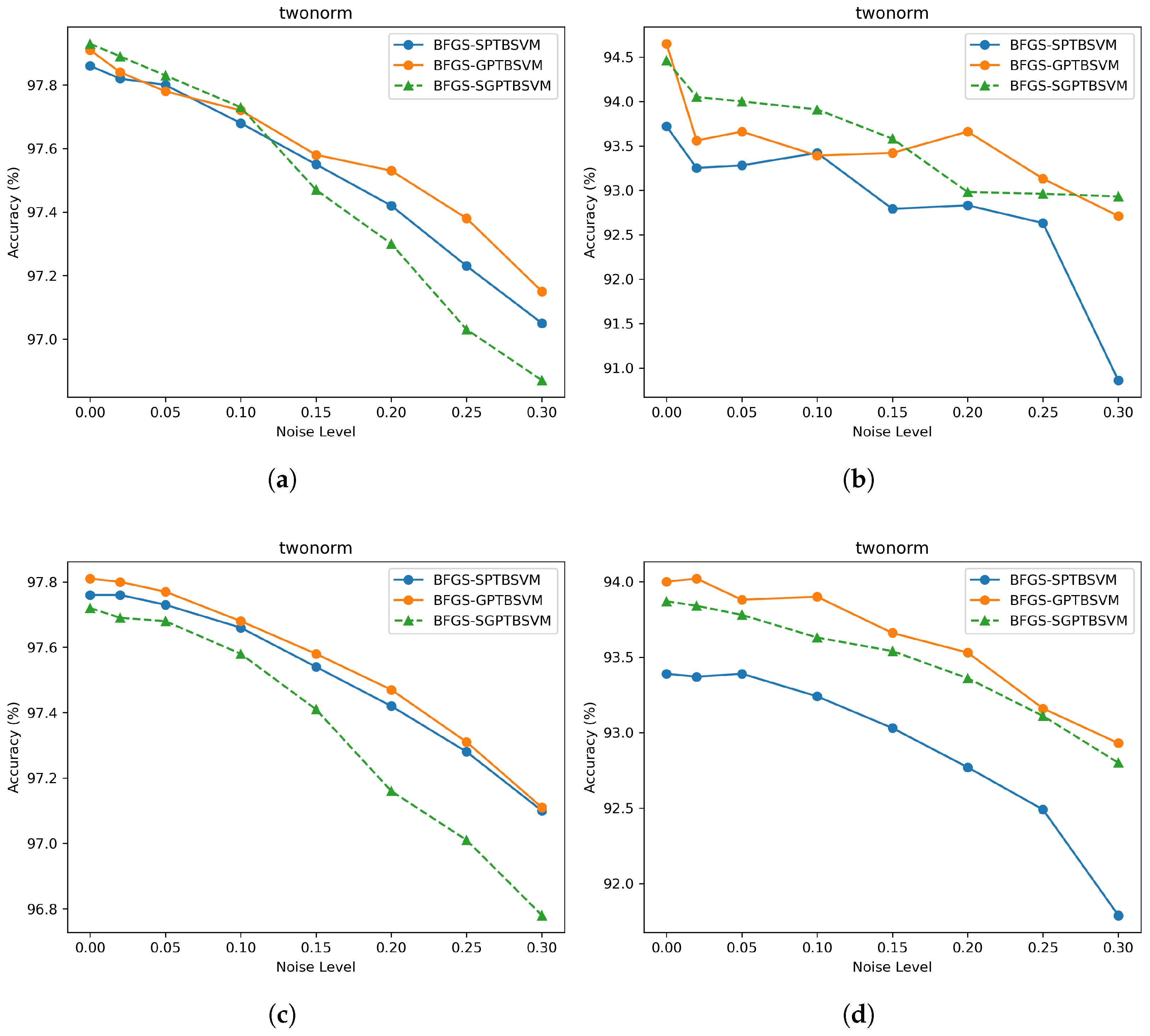
As the Twonorm dataset is the dataset that gives the best performance, its results are presented first. Figure 2 shows the performance of the BFGS algorithm applied to the TBSVM model at different noise levels. Loss functions implemented are our proposed loss (labeled BFGS-SGPTBSVM in the figures), the generalized pinball loss (BFGS-GPTBSVM), and the smooth approximation to the pinball loss (BFGS-SPTBSVM).

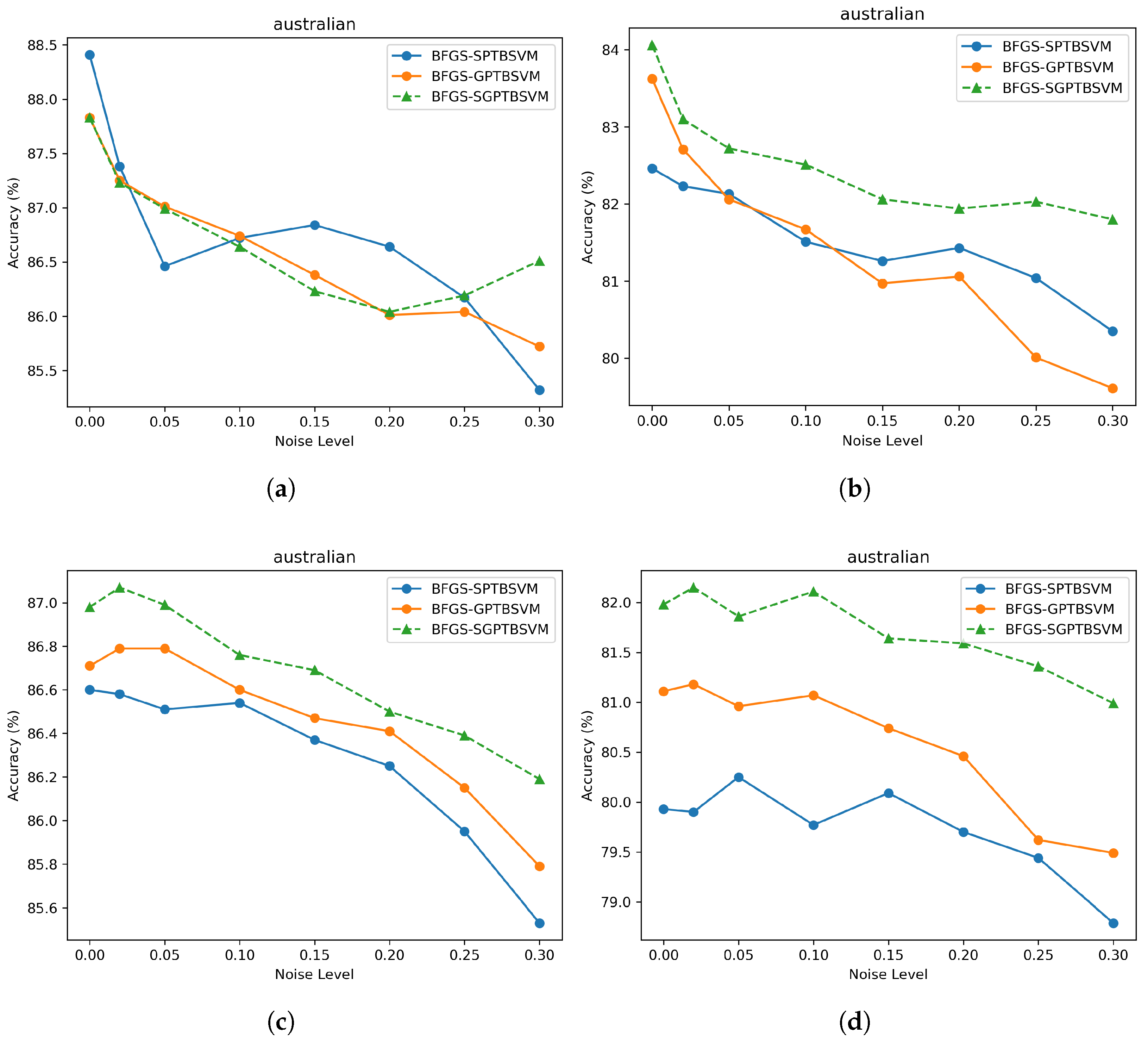
From Figure 2, we observe that as noise increases, the accuracy of all algorithms tends to decrease. Figure 3 shows the performance of different noise levels for the Australian dataset. We observe that, overall, our smooth generalized pinball loss function retains the noise insensitivity property of the generalized pinball loss function and shows lower noise sensitivity on the Australian dataset in most cases.

The experimental results indicate that the proposed method exhibits stable performance across repeated runs, as reflected by relatively small standard deviations. Moreover, the smoothing parameter $\mu$ allows a controlled trade-off between approximation accuracy and numerical stability. While the proposed smooth generalized pinball loss involves higher-order polynomial terms and may introduce additional per-iteration computational cost compared with simpler pinball losses, the resulting twice differentiable objective function guarantees efficient quasi-Newton optimization. This partially compensates for the increased complexity, leading to acceptable overall training times.

Although widely used, the UCI benchmark datasets may not fully reflect the complexity of highly structured, large-scale, or application-specific data. Therefore, the reported experiments primarily serve to validate the general effectiveness and stability of the proposed loss function. Future work will investigate the performance of the proposed approach on more challenging datasets, including imbalanced and domain-specific problems.

5. Conclusions and Discussion

This paper has introduced a family of smooth generalized pinball loss functions to address the issues associated with non-differentiability found in traditional loss functions, such as the hinge loss, pinball loss, and generalized pinball loss function. In addition, a novel twin-bounded support vector machine model with a smooth generalized pinball loss function is proposed. We proved that the generalized pinball loss function can be approximated by the proposed smooth generalized pinball loss function in the uniform norm with arbitrary precision, and that the solution of our TBSVM model is unique and converges to that of the non-smooth problem. In experiments, we selected nine UCI datasets and used a quasi-Newton method to solve the corresponding strongly convex unconstrained optimization problems with twice continuously differentiable objective functions. We then compared the proposed BFGS-SGPTBSVM algorithm with BFGS-GPTBSVM and BFGS-SPTBSVM algorithms in terms of classification performance, accuracy, and computational speed. From the numerical experiments, we found that the proposed BFGS-SGPTBSVM algorithm shows the best performance for the TBSVM with RBFSampler.

The proposed smooth generalized pinball loss-based TBSVM is particularly suitable for classification problems involving noisy, imbalanced, or asymmetric data distributions, where robustness and stable optimization are critical. For problems requiring explicit physical constraints or domain-specific modeling, hybrid loss formulations may be more appropriate.

In future studies, we plan to assess the performance of our model by experiments with complex, large-scale datasets. Moreover, we will evaluate sensitivity to hyperparameters and improve the techniques of parameter optimization for speed and efficacy enhancements. Finally, we will further apply our proposed loss function to other support vector machine models.