


Abstract
There are several drawbacks in the existing localization (active contour) models. Some models have poor capability of handling uneven illuminations and low contrasts, others are sensitive to initial condition, and there are still some models which can not converge to the object boundary stably. In this paper, following the routes of Localizing Region-Based Active Contours (LRBAC) which is an important localization method, we propose a new localized active contour model. By altering the underlying construction logic, our proposed algorithm overcomes the problem of LRBAC with respect to poor convergence stability. Compared with some state-of-the-art localization models, our new algorithm is more similar to an edge-based one and therefore performs better when handling uneven illuminations and low contrasts. Moreover, combining the features of the region-based and the edge-based active contours, we propose, for our algorithm, a simple approach to dynamically control the localization size. This dynamical method makes our algorithm more robust to the initial condition. Detailed theoretical analysis and comparison are presented to clarify the features of our proposed algorithm. Experimental results on real-image segmentation underline the effectiveness of our proposed algorithm.
MSC:
68T45; 68U10
1. Introduction
Active contours, often referred to as “snakes,” are a prominent image segmentation or object recovery method that have gained widespread popularity over recent decades. A snake is defined as a closed curve within the image domain. This curve dynamically deforms and evolves, based on specific dynamical equations, ultimately arriving at the boundary of object and separating the foreground (object) from the background. Additionally, it can also partition images into several regions characterized by homogeneous features, such as intensity, color, or texture.
The dynamical equation driving the curve deformation is typically derived from the gradient flow of an energy functional. This equation primarily encompasses two terms: the smoothing term and the data term. The smoothing term, determined by the curve’s geometry, ensures the active curve’s smoothness. Conversely, the data term, determined by the image content, guides the curve towards object boundaries.
According to the image content (or information) utilized to construct the data term, active contours can be classified into two categories: edge-based and region-based. Edge-based snakes [1,2] rely on some local information such as the stark differences or significant image gradients to frame the data term. On the other hand, region-based snakes [3,4,5] leverage more global information, like feature distribution within image regions, to craft the data term.
Due to the characteristics of the utilized image information, edge-based and region-based snakes offer distinct advantages and challenges. Firstly, edge-based snakes can accurately capture the object boundaries and demonstrate resilience to uneven illuminations [6] appearing in images. However, due to just using the local information of images such as the image gradient, edge-based snakes remain susceptible to noise and texture, often necessitating delicate initialization. Comparatively, due to using more global information of images, region-based snakes demand less stringent initial conditions, exhibit robustness against noise, and can recover objects with faint or even absent edges [3]. However, region-based snakes might produce inaccurate segmentation results when the object and background share similar features. Moreover, they struggle to delineate object boundaries in images with uneven illuminations [6].
For enhanced robustness against initialization and noise in edge-based snakes, various external force fields have been introduced [7,8,9,10,11,12,13,14,15]. Numerous energy functionals and region descriptors have been conceived [16,17,18,19,20,21,22,23,24,25,26] to address unique challenges like texture and clutter segmentation. Some studies proposed control terms [27] to guide snake movement and enhance segmentation outcomes. The inclusion of object shape priors in specific algorithms [28,29,30,31,32] augments segmentation accuracy, especially when relying solely on image features like intensity or color, proves insufficient.
Furthermore, numerous efforts aim to merge the benefits of region-based and edge-based methods. Among them, some strategies [33,34,35,36,37,38,39] suggest combining various modules to formulate the energy functionals. These modules are distinctly crafted using either edge or region information. Given that these modules are based on different prior assumptions, there can be instances where the derived data terms clash [12].
Advanced integration techniques in recent years have been termed “localization methods.” These methods have garnered significant attention in the realm of image segmentation [40]. A defining feature of localization methods is their reliance on a limited set of local data surrounding the snake for driving the motion of a region-based snake.
C. Li et al. [41] introduce the Region-Scalable Fitting (RSF) model to address the challenges posed by uneven illuminations (or called intensity inhomogeneities) in images. They expand on this with the Local Intensity Clustering (LIC) model, incorporating a bias-correcting operator to rectify uneven illuminations [6]. Following the way of RSF and LIC, a lot of localization models are later proposed. In these models, the constructed energy functionals are determined by every pixel in images, similar Gaussian functions and bias-correcting operators are used to realize the localization of snakes and rectify uneven illuminations. For example, K. Zhang et al. [42] adapt the bias-correcting operator for their model, using both mean and variance as region descriptors. The Local Approximation of Taylor Expansion (LATE) model, aiming to approximate uneven illumination variances through a nonlinear approach, is proposed in [43]. Innovations also emerge by integrating fuzzy cluster analysis [44] and fractional order differentiation [45] into localization methods. These models improve active contours in handling uneven illuminations. However, they are sensitive to initialization since only local information is used to guide the curve evolution [46]. In order to overcome this problem, Wang et al. propose [46] a multi-scale level set model based on the bias-correcting operation, which uses multi-scale low-pass filtering to statistically analyze the local image intensity in circular shape and approximates the local image intensity using piecewise constant interpolation. Recently, Q. Cai et al. [47] propose an Adaptive Variational Level Set Model (AVLSM), in which an adaptive scale bias field estimation term and a variation-based denoising term are presented for handling severe intensity inhomogeneity and high noise. These models using variable scales promote the robustness of localization methods for initialization, but the computational complexity also largely increases.
In addition to RSF, LIC, and their inspired models, algorithms like the one in [48] delve into local region descriptors in detail. The intriguingly named “curious snake” model [49] utilizes local and global data for segmenting images with cluttered backgrounds. Some post-processing and hybrid procedures have also seen the integration of localization methods. For instance, H. Wu et al. [21] utilize global image data to form an energy functional before opting for local data in the snake evolution process. In [50,51], refinement terms based on local information are added to enhance the segmentation accuracy of some snakes driven by global information. However, these models still use fixed scales to control the size of the local image data driving curve evolution (termed the “localization size”), so they are also sensitive to initialization. In addition, a simple hybrid of the local and the global region information faces the problem where the derived data terms clash, just like those early models using edge and region information.
Another notable method is the Localizing Region-Based Active Contours (LRBAC) developed by S. Lankton and A. Tannenbaum [52]. Unlike RSF and LIC, LRBAC just extract a set of local data near the active curves to construct the energy functional. In addition, LRBAC uses a characteristic function, rather than the Gaussian function, to realize the localization of the snake. Due to just using local data rather than global data contained in images to construct their energy functional, LRBAC is more similar to an edge-based method and so performs with a better ability to handle uneven illuminations. However, LRBAC faces issues with convergence stability and initialization sensitivity [21,52], hampering its broader application.
In this study, we primarily emphasize unsupervised methodologies, aiming to develop a more efficient algorithm to overcome the problems of the existing localization methods. For dealing with uneven illuminations better, we adopt the same technical route that LRBAC [52] has to construct our model. However, by altering the fundamental construction logic, our proposed snake overcomes the problem of LRBAC with respect to convergence stability (refer to Section 3 for details). Compared with those state-of-the-art snakes such as RSF [41] and the more recent LATE [43] and AVLSM [47], our proposed algorithm is more similar to an edge-based method (just like LRBAC), so it has a better capability of handling uneven illuminations and low contrasts. Furthermore, our snake just has one data term, so it does not face the problem of data term clash. Finally, by harnessing the strengths of both region-based and edge-based methodologies, we propose a variable scale method to dynamically control the scope of the extracted local data i.e., the localization size of our algorithm. This dynamical method ensures our snake’s robustness to initialization.
The primary contributions of this paper are delineated below:
- 1.
- By altering the underlying construction logic, we resolve the persistent issues of poor convergence stability inherent in LRBAC presented in [52].
- 2.
- We introduce a more straightforward yet efficacious approach to dynamically resize the localization size, improving the robustness of the localization methods to initialization.
- 3.
- Based on the two works above, we propose a new localization snake algorithm which shows superior performance over the state-of-the-art localization models such as RSF [41], LATE [43], and AVLSM [47] in accuracy, especially in scenarios with severely uneven illuminations and low-contrast images.
We would like to highlight that our proposed method is traditional and foundational, and primarily driven by an a priori assumption or principle. Over recent years, many segmentation algorithms based on artificial neural networks have emerged. Notable examples include [53,54,55,56]. These algorithms have achieved significant milestones in their respective domains, although their needs for large-scale datasets make them limited by the lack of enough labeled samples used for training [47]. Potential extensions of our proposed algorithm are eagerly anticipated, especially when integrated with big data-driven neural network methods. Such integrations have already been explored in studies like [57,58].
The structure of this paper is delineated as follows: Section 2 reviews several localization models related to the proposed algorithm. Section 3 introduces a localized snake algorithm, discussing its unique characteristics and how it differs from existing methods. Section 4 presents experiments conducted on real image segmentation to validate the efficacy of our proposed algorithm. Finally, conclusions and discussions are reserved for Section 5.
2. Background
In this section, we provide a concise overview of four representative localization models. Let denote the domain of an image . Here, represents the image feature space, which can be, for instance, the intensity. To streamline our discussion, we focus predominantly on the two-phase segmentation, where the aim is to segregate the image into the object and the background. In the field of active contours, when the (initial) closed curve deforms according to specific kinetic equations and arrives at some locations where the driving force is zero, the curve rests, then the interior region of the curve is just the recovered object (foreground) and the exterior region of the curve is the background.
2.1. RSF
The Region-Scalable Fitting (RSF) method, introduced in [41], remains a leading-edge algorithm, primarily due to its straightforwardness and effectiveness. The core of RSF lies in its energy functional, formulated as
where is a binary level set function as described in [59]. The zero level set of , denoted by , implicitly encapsulates a closed curve. Within , we have , and outside , . The Heaviside function, , is defined as
represents the Dirac delta, acting as the generalized derivative of the Heaviside function shown in (2). represents a Gaussian kernel function given by . The spatial variables and are independent. With the Gaussian kernel’s intervention, for every coordinate , only the neighboring pixels defined by play a dominant role in the evaluation of energy (1). Lastly, the term calculates the arc length of ’s zero level set.
Using the calculus of variations, one can determine that for a fixed , the optimal functions and that minimize Equation (1) are given by [41]:
and
Given functions and , one can evolve as per the following equation to minimize (1) [41]:
The energy terms are defined as
The Gaussian kernel, , serves as a localization operator. Thus, the data term in (5) is driven primarily by local data within images, especially, by the local data surround the zero level set of . Here, , representing the curvature of the zero level set. The term acts to penalize the arc length and maintain smoothness in the zero level set. The parameter controls the extent of the arc length penalty.
2.2. LATE
Building upon the RSF methodology, the Local Approximation of Taylor Expansion (LATE) method is introduced in [43]. It introduces the following energy functional:
Here, the terms , , , and are the same as those in the aforementioned RSF model. and represent the intensity means of the local regions and , respectively. In detail,
where the symbol denotes a neighborhood around the point , while (with ) signifies the interior and exterior regions of the curve . The function describes the bias field, capturing the intensity inhomogeneity (or uneven illumination) variation in images. and , respectively, define the region descriptors of and .
Using the calculus of variations, one can determine the optimal values for , , and . The derivations and expressions for , , and are detailed in [43], as shown in Equations (9)–(11).
where
Finally, evolving according to the following equation can minimize (7):
2.3. AVLSM
In [47], Q. Cai et al. propose an Adaptive Variational Level Set Model (AVLSM), which introduces an adaptive localization size and a variation-based denoising (VBD) term into the original LIC model [6] in order to handle severely uneven illuminations and high noise. AVLSM presents the following energy functional [47]:
where is a positive weight controlling the contributions of different terms. is an adaptive scale bias field estimation term
where
In the equation above, is a slowly varying bias field estimation function for correcting the uneven illuminations of images, , which are, respectively, the level set function and the Heaviside function (the same as those in the aforementioned RSF model). and are constants describing the image intensity in a local region controlled by the adaptive scale truncation function , and
is an adaptive scale Gaussian truncation function.
is the adaptive scale, where and are two positive constants which are related to the image size. is the image entropy. in (15) is a variation-based denoising (VBD) term. In detail,
where , , and are balancing factors controlling the weights of different terms. is the Dirac delta function. e is the edge detection operator:
Finally, is an energy penalty term used to avoid complex and time-consuming re-initialization during curve evolution, and is defined as
where is a positive constant and is the energy density function
In order to minimize (15), the Euler–Lagrange equation and gradient descent flow are used. In detail, keeping all the parameters fixed and minimizing the above equation with respect to , the final iteration formulation is obtained [47] as follows:
where ∗ denotes convolution operation. Using
to compute the clean image. Keeping and fixed and minimizing (15) with respect to parameters , , and b, respectively, we obtain their update formulas as [47]:
and
2.4. LRBAC
Another localization method attracting significant attention is the Local Region-Based Active Contours (LRBAC) framework proposed by S. Lankton and A. Tannenbaum [52]. The following energy framework is described in [52]:
where is the binary level set function and is the Dirac delta function, just as introduced in the aforementioned RSF model. is a localization operator defined in terms of a radius parameter r:
In this framework, and are independent spatial variables, and the function F represents local adherence to a given model at each pixel along the contour [52]. Due to the roles of and the localization operator , it is just a set of local data surrounding the curve that determines the energy (29). This treatment of LRBAC is different to RSF, LATE, and AVLSM mentioned above.
By applying the first variation calculus to Equation (29) and considering the gradient flow as the driving force, we derive the following time-dependent evolution equation as described in [52]:
To simplify the equation further, we move the term outside of the integral, leading to a reformulated version of Equation (31) as follows:
In this reformulated representation, the term serves as a localized energy metric, which is evaluated based on the data surrounding the point .
3. The Proposed Algorithm
3.1. Methodology
Edge-based snakes just take local information of images to construct their energy functionals and they are insensitive to uneven illuminations compared with region-based ones. For making our proposed snake more similar to an edge-based one and giving it a better capability of handling uneven illuminations, we follow the way of LRBAC [52] to construct our energy functional. However, we will compute the discrepancy of the extracted local data, rather than computing some respective homogeneities as LRBAC proposed (more details will be presented in Section 3.2 and Section 3.5). The traditional curve evolution method is used to minimize the constructed energy. However, we will propose a dynamic method to change the size of the extracted local data, i.e., the localization size of our algorithm. The dynamic method improves the robustness of our snake to initialization.
Specifically, we undertake the following steps to construct our snake algorithm. Given a closed curve within the image domain:
- 1.
- Local Data Extraction: We start by extracting a comprehensive set of local data surrounding each pixel on the curve. This data is subsequently divided into two distinct parts based on the orientation and structure of the closed curve itself.
- 2.
- Feature Evaluation and contrast: We compute certain statistical parameters within the two divided parts to evaluate their respective characteristics, and by computing the distance between the parameters, the differences in features between the two parts are evaluated.
- 3.
- Integration and Functional Proposal: The evaluations obtained from the entire curve are integrated to provide a cohesive perspective. Based on this, we propose an energy functional intrinsically determined by the curve’s location.
- 4.
- Energy Minimization: We employ curve evolution methodologies to minimize the aforementioned energy. These techniques ensure the curve converges toward an optimal configuration.
- 5.
- Dynamic Resizing during Evolution: As the curve evolves, we dynamically resize the scope of the local data. This ensures that the more relevant and suitable data is chosen, enhancing the algorithm’s robustness to initialization and segmentation accuracy.
3.2. Construction
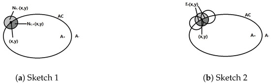
Consider a closed curve defined in the image domain (refer to Figure 1 for comprehension). This curve can be represented as
Figure 1.
In (a,b), AC denotes the active closed curve (i.e., ); the small disc with dark and light shadows denotes ; and are, respectively, the interior and exterior regions of the active closed curve. In (b), the union of the three discs denotes .
Here, s denotes the arc length parameter. One can assume that this closed curve, , is the zero-level set of a binary function [3,41,59] such that
Further, it is assumed that
where and are the global interior and global exterior of , respectively.
For any pixel located on , a closed neighborhood with radius r is defined as
This radius is actually dynamic. We will present how it changes later.
In the above equation, represents a second set of spatial variables, distinct from . The neighborhood is further split into two segments: the local interior and the local exterior . This segmentation uses the closed curve itself (see Figure 1a for reference).
The average intensity distributions inside and are computed as
and
where denotes the measure.
Introducing a localization operator:
where H denotes the Heaviside function (the same as that in (2))
we can re-express Equations (37) and (38) as
To evaluate the disparity in characteristics between and , we use
The bigger the disparity between and , the smaller the value of .
Remark 1.
Here, we propose to evaluate the disparity in characteristics between and using (45), rather than to compute the respective homogeneities within and as LRBAC [52] provides. This is due to the following intuition: under certain circumstances, the reasonable snake evolution may lead the local energy which computes the respective homogeneities to non-monotonic change. As a result, the gradient flow of the energy could not drive the snake evolution to the object boundary stably. For example, consider the localized Chan–Vese energy presented in [52]:
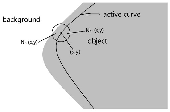
where the optimal and , which minimize , are, respectively, the intensity means and expressed in (43) and (44). When the active curve is located in the position shown in Figure 2 and moves to the edge of object and background, the local energy could not keep decreasing monotonically. For simplicity of discussion, we assume that the image is binary, the intensities of the object and the background are, respectively, 0 and 1. When the active curve moves to the edge, and the local variance remain unchanged. While will change from 0 to 1 and the other local variance will first increase from 0 to , then decrease from to 0. So, the energy will first become bigger, then become smaller. On the other hand, we can see that during the evolution of the active curve to the edge, our proposed energy always becomes smaller (from 0 to ). Those intuitions inspire us to construct the new localization algorithm and overcome the problem of LRBAC.
Figure 2.
A sketch map. Here, the image is binary: the intensities of the object and the background are, respectively, 0 and 1. When the active curve evolves to the edge of the object and background, the intensity mean within (i.e., ) and the localized variance are both equal to 0 and remain unchanged. Yet the intensity mean within (i.e., ) will change from 0 to 1 and the localized variance will first become bigger (from 0 to ), then become smaller (from to 0). So, the localized energy will also first become bigger, then become smaller. On the other hand, during the snake evolution, our proposed local energy always becomes smaller (from 0 to ).
To integrate this disparity over the curve , we employ the Dirac delta function:
In this study, we address the minimization of (47) as a key criterion for image segmentation. Notably, the influence on (47) primarily comes from the local data around the contour , rather than the broader, global data spanned across the image. As a result, the energy functional typically settles into its local minimum. This inherent limitation of (47) mirrors the challenges encountered with traditional edge-based algorithms. However, the dynamic adjustment of localization size, discussed in Section 3.4, and the impressive segmentation performance of the proposed algorithm counterbalance this limitation. Moreover, the function is always non-positive; this ensures that 0 is the global maximum of (47). This intrinsic characteristic precludes the curves from degenerating to a mere point, a problem frequently seen in edge-based snake techniques.
To enhance the curve’s smoothness in the model, we incorporate an arc length penalty into Equation (47):
where stands for a positive parameter that dictates the strength of the arc length penalty. For this study, we set .
3.3. Energy Minimization
In our study, we employ a conventional gradient descent methodology to minimize the energy function as denoted by Equation (48). In detail, we first initialize a binary function (whose zero level set is a closed curve in image domain), then we evolve along the gradient flow (negative gradient field) of (48) until (48) obtains its minimal (where the gradient of (48) is equal to zero).
Utilizing the principles from the calculus of variations, the gradient field of Equation (47) is derived and can be found in Appendix A. This gradient field is expressed as
On the other hand, for the arc length penalty in (48), the following relationship can be readily derived as follows:
where the curvature, , is given by
and the function represents the divergence operator. To progress further, we deform the function along its gradient flow (negative gradient field) of Equation (48):
3.4. Setting a Dynamic Localization Size
As the most important parameter of our proposed algorithm, the localization size, specifically the neighborhood radius r, dominates the performance of our algorithm. Specifically, if r is set too small, it fails to encompass significant portions of the object boundary. This results in the acquired region data inadequately representing the feature variations near the object boundary. Consequently, the algorithm is prone to ensnaring in undesirable local minima, leading to premature segmentation outcomes. This issue is akin to the “poor capture range” problem [7], a challenge many edge-based snake algorithms face. In contrast, while increasing the value of r might mitigate the local minima issue, it may result in imprecise boundary delineations. Notably, incorrect segmentations are frequently observed in instances of uneven illumination within the images under consideration. This challenge is a familiar shortcoming of numerous region-based snake algorithms. For a more comprehensive exploration, refer to [6,21].
A dynamic adjustment of r is proposed to navigate this conundrum. The existing dynamic adjustment methods are inclined to set the scale r based on some extra criterions which are independent of the introduced data terms [47]. These dynamic methods are essentially the combinations of different segmentation criterions. It will result in instances where different segmentation criterions clash [12].
In this paper, we tend to introduce a dynamic adjustment method of r, just based on the characteristics of the region-based and the edge-based methods. First, at the inception of snake evolution, r should be assigned a relatively large value, allowing the snake to evolve like typical region-based algorithms. This ensures a stable progression towards the object boundary. As the snake draws closer to this boundary, r gradually reduces. Ultimately, r diminishes to a relatively low value, prompting the snake to operate like an edge-based algorithm. This dynamic method facilitates more precise boundary detection, especially in uneven illuminations in the images.
To elucidate in detail:
1. Initiate with . 2. After each iteration (or a set number of iterations), update r using the formula . 3. If the right side of Equation (52) equals zero, then update , followed by the execution of the succeeding evolution of (52). 4. On reaching the condition where and the right side of Equation (52) equals zero, the snake evolution is terminated and the segmentation result is presented.
The specific assignment for is predominantly influenced by the degree of uneven illuminations in the images. For images with minimal uneven illuminations, can assume a higher value, such as or , where m and n represent the image’s row and column counts, respectively. However, in cases of pronounced and erratic illuminations, a smaller , such as or , is more apt. It is also advisable to position the initial curve proximate to the object boundary under these conditions. The parameter , on the other hand, is largely dictated by the faintness of the desired edges. Fainter edges typically necessitate a reduced value. In the majority of the experiments discussed in this paper, we opted for and values approximating and , respectively.
3.5. Analysis and Comparison
3.5.1. Comparison with LRBAC
The construction technique of our proposed algorithm shows parallels to the LRBAC framework. Specifically, both methods utilize a set of local data surrounding closed curves to formulate the energy functionals. Furthermore, they employ an akin localization operator. Nevertheless, pivotal differences distinguish our proposed algorithm from the LRBAC framework.
- Rather than evaluating the individual homogeneities of two neighborhoods, our approach focuses on discerning the feature differences between and .
- A dynamic method of localization size is proposed to improve the algorithm’s robustness to initialization.
Items 1 and 3 above are straightforward. Now, we focus on discussing the second item. Building on the template provided by (32), in [52], S. Lankton et al. rewrite some models using the template. Here, we select the rewritten Mean Separation (MS) Energy model [60] for further discussion. The rewritten MS model (removing the smoothing term) has a following evolution equation [52]:
Firstly, due to stemming from different energy functionals, the evolution Equations (52) and (53) have different computational mechanisms inside the integrals. Most interestingly, in (53), the spatial variable positions of and are the inverse of those in (52). This mathematical discrepancy leads to distinct data collection methods between (53) and (52). In particular, when calculating the right side of (53), the region data, from which and are derived, originates from (see Figure 1a). Additionally, due to the influence of and , pixels along the curve segment (see Figure 1b) also play a role in determining the value of (53). We think that this data collection strategy results in (53)’s subpar convergence stability. It is due to the fact that when the image contains uneven illuminations or r is set a larger value, the features on the curve segment have large discrepancies, using these discrepant features to determine the level set function’s evolution at and the classification of pixel greatly increases misclassification risk. Notably, in [52], all models reshaped by the LRBAC framework exhibit a data collection mode similar to (53). To achieve optimal segmentation, one often needs a meticulous localization size and initial condition [21,52], narrowing the LRBAC framework’s broader applications and limiting further studies.
Contrastingly, (52) avoids such issues. The region data, from which and in (52) are determined, arises from (see Figure 1b). With a consistent r, this set is more expansive than , with the latter being a subset of the former. For a smaller r, collecting more data can mitigate convergence to unwanted local minima. Moreover, aside from the region data, only the feature of pixel (represented by ) determines (52)’s right side. This ensures that regardless of r’s size, the pixel’s classification hinges only on the pixel itself, bolstering algorithmic convergence stability and significantly lowering misclassification risk. Such a data collection strategy allows a dynamic localization size for our algorithm’s data term.
3.5.2. Comparison with RSF, LATE and AVLSM
Recall the RSF energy functional, as shown in Equation (1) (the arc length term is omitted for the sake of simplicity). The functional is expressed as
where is the Gaussian kernel function.
For any point , we can compute a local energy contribution as
This local energy, computed using the neighboring data around the point , contributes to the overall RSF energy functional. It implies that the RSF approach fully utilizes the entire image data to construct its energy functional.
In contrast to RSF, our proposed energy functional, given in Equation (47), considers only the local data near the closed curve, primarily due to the presence of .
Similarly, the difference between our method and RSF is manifested in the evolution equations as well. Recall the RSF evolution equation,
Due to the role of the Gaussian kernel , only when , the two means and provide a non-zero contribution to the evolution equation. This indicates the collection scope of the region data of (56).
In our proposed algorithm, the Dirac delta function and the ball confine the effective data to a smaller subset, (Figure 1b), which is a (linelike) subset of . In detail, only when , the two means and provide a non-zero contribution to our evolution Equation (52). So, we can see that the collected region data of our algorithm is closer to the active curve than RSF.
These distinctions indicate that our proposed algorithm is more “edge-based” than RSF, offering improved performance for handling images with uneven illuminations.
Regarding localization operators, RSF employs a Gaussian kernel , which rapidly diminishes as the distance between points increases. In our model (and LRBAC), is selected as the localization operator. For all of subjected to , . In other words, the pixels subjected to present equal contribution to the relative calculations.
LATE and AVLSM follow the footsteps of RSF (and LIC [6]) in terms of energy functional construction, where every pixel contributes to the energy. These three algorithms employ the same localization operator. So, our proposed algorithm is also more “edge-based” than LATE and AVLSM. Additionally, compared to LATE and AVLSM, our algorithm involves fewer parameters and terms in the evolution equation, making its computational efficiency higher than LATE and AVLSM.
3.6. Numerical Implementation
The implementation of our method is straightforward. We use the finite difference method to solve the partial differential Equation (52). First, we discretize (52) and then obtain an iteration scheme:
where and are, respectively, the data and the smoothing terms of (52), i.e., the first and the second terms of (52). is the time step. Here, is discretized as a signed distance map [61]. We point out that using the binary step function and the Distance Regularized Level Set Evolution (DRLSE) methods [61] would greatly reduce the computational cost and make the algorithm significantly faster. The computation of and in the smoothing term of (52) is simply discretized as central finite differences. Given an initial level set function , implementing the iteration scheme (57) until the energy difference or the number of iterations is equal to p can obtain the numerical solution of (52), where and p are two preset parameters.
The main computational cost in our proposed algorithm is to compute the data term. Now, we provide the detailed method of computing the data term. Considering the data term expressed as
First,
and
are, respectively, selected as the smooth approximations of the Heaviside function and the Dirac delta, where is a small constant. Following that, for the given , the two local means (refer to (43) and (44))
and
can be computed by the following convolutions:
and
where ∗ denotes the convolution operator, I is the input image, and 1 is a matrix with the same size as I, whose entries are all equal to 1.
Now, we initiate a subtle modification to the representation (58). Specifically, for computational simplicity and stability, we adjust the terms and from Equation (58) to be equivalent constants. In the context of this paper, we set both to unity, that is, .
This adjustment arises from practical considerations: in numerical computations, and are the numbers of pixels determined within and . Large values from this computation can diminish the data term significantly, resulting in a sluggish curve evolution. Although one approach is to normalize these terms using the ratios and , this normalization increases convolution operations, making the process more computationally demanding compared to setting them as constants.
Upon implementing the above adjustments, our expression becomes
This can be equivalently expressed in terms of convolutional operations as
In the above computation of the data term, for one input image, the two convolutions and just need to be implemented once before the iterations. Due to depending on the evolving , the other four convolutions including , and the two convolutions in (66) need to be computed at every iteration. Finally, we point out that for all the convolution operations presented, the kernel can be approximated using a matrix (or mask) with each entry being 1. As the algorithm progresses, the value of r is reduced by one either in each iteration or every few iterations until it reaches a steady constant value . It is worth noting that an approximation using a matrix can also be employed for a continuous adaptation of the mask size without any significant impact on the algorithm’s performance.
4. Experimental Results
In this section, we present an extensive experimental analysis to validate our proposed algorithm’s performance in real-world image segmentation tasks. This section is organized into two distinct subsections.
In the first subsection, we rigorously evaluate the adaptability of our proposed algorithm in handling complex challenges commonly found in real-world scenarios, such as noise, low contrast, and uneven illumination conditions. To ensure an objective comparison, we also incorporate existing state-of-the-art algorithms, namely the LRBAC, RSF, LATE and AVLSM into our experiments. In addition, we add a deep learning segmentation model, DARNet [57], in our experiments. Specifically, Equation (54) serves as the data fidelity term for the LRBAC framework. For the Gaussian kernels employed in both RSF, LATE, and AVLSM, we follow the truncation scheme presented in [41], where the kernel is truncated to form a matrix (mask). Here, represents the standard deviation of the Gaussian function. We will also set different values for in order to obtain the better experimental results. Moreover, unless otherwise specified, the two localization parameters and in our proposed algorithm are set to and , respectively. Here, m and n are, respectively, the numbers of the rows and the columns of the input images.
In the second subsection, we design experiments focusing on the sensitivity analysis of two pivotal parameters, and , in our proposed algorithm. We systematically explore their impact on the algorithm’s performance, thereby identifying the robustness of our proposed algorithm to these two parameters.
It should be noted that for all the experiments conducted, we directly applied the various algorithms to the raw images without any pre-processing steps like smoothing or normalization, maintaining the integrity of the test conditions. Finally, all these numerical experiments are conducted in MATLAB (R2019a) on a Windows 11 (64 bit) notebook computer with an Intel Core i5 2.40 GHz processor and 16 GB of RAM.
The source code for our proposed algorithm is openly accessible. Interested parties can contact the first author of this paper (Q. Li) to obtain the code and further evaluate its efficacy on diverse datasets.
4.1. Abilities of Segmentation
Medical images, such as Computed Tomography (CT) and Magnetic Resonance Imaging (MRI), often exhibit uneven illuminations and low contrasts between objects and backgrounds. These present considerable challenges for image segmentation techniques, particularly for the region-based snakes. This section will delve into a series of experiments that focus on segmenting medical images with uneven illuminations and low contrasts. Several experiments on normal optical image segmentation are also presented to test our proposed algorithm’s ability to handle other real images.
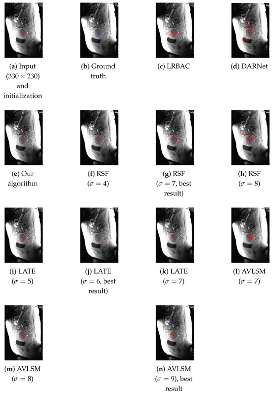
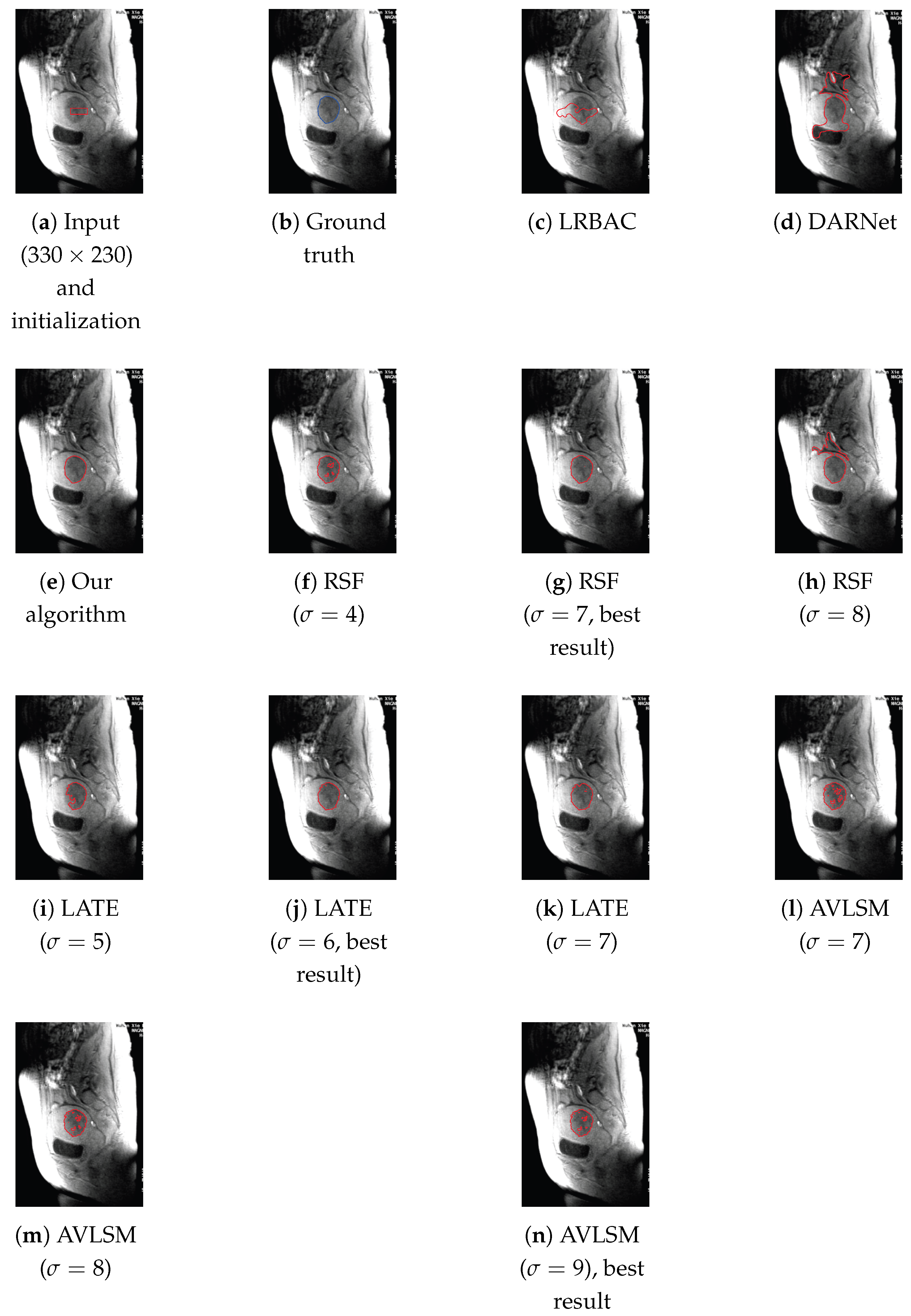
The initial experiment revolves around the recovery of a tumor, as illustrated in Figure 3. This input image (Figure 3a) suffers from uneven illumination and features the tumor object with a low contrast compared to its neighboring regions. LRBAC exhibits weak convergence stability when initialized as depicted in Figure 3a. This lack of stability causes LRBAC to falter, stopping at the position shown in Figure 3c, ultimately failing to complete the segmentation task. DARNet presents a leaked boundary (Figure 3d). When setting , the RSF method results in fragmented segments, as seen in Figure 3f. It is only when that RSF successfully segments the image without fragmentation, as shown in Figure 3g). However, with , RSF produces a leaked object boundary (the program is terminated after 1000 iterations to prevent the active curve from further leaking), evident in Figure 3h. We experiment with values of 5, 6, and 7 for the LATE method. Out of these, only yields a reasonably accurate outcome, as demonstrated in Figure 3j. When setting for AVLSM, reasonable boundary recoveries are presented, but many islands always appear in the recovered object.
Figure 3.
Results of different algorithms on the recovery of one tumor: (a) the input image and the initial curve location, (b) the ground truth boundary of the object (identified by the blue curve), (c) the segmentation result given by LRBAC, (d) the result given by GARNet, (e) the result given by our algorithm, (f–h) different results given by RSF with different settings of the parameter , (i–k) different results given by LATE with different settings of , and (l–n) different results given by AVLSM with different settings of . In (c,d,h), the programs were terminated manually after 1000 iterations (to prevent the active curves from further leaking). For RSF, LATE, and AVLSM, the best results are measured by Dice.
Comparatively speaking, our newly proposed algorithm effectively mitigates the effects of uneven illuminations and weak edges, ultimately achieving a precise object recovery, as seen in Figure 3e. Notably, the boundary identified by our method is considerably smoother than those obtained using the RSF with and LATE with and AVLSM with all the settings of .
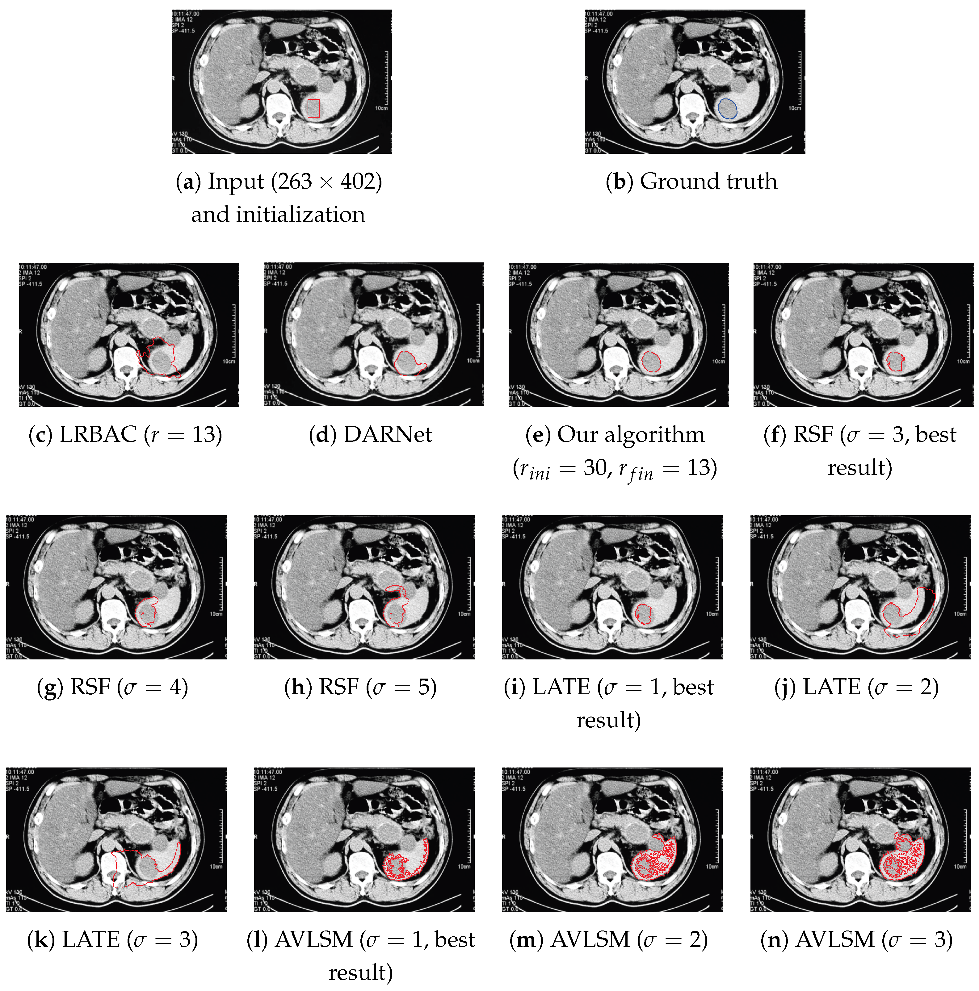
In the second experiment, as depicted in Figure 4, our main objective is to test the ability of our proposed algorithm to handle situations with low contrasts. Specifically, in this experiment, a tumor is the target object to be recovered. This tumor and its neighboring regions present a lower contrast, primarily due to the strong noise.
Figure 4.
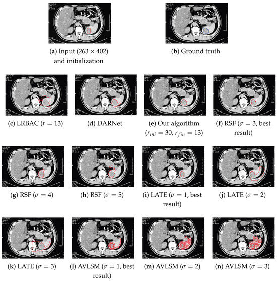
Results of different algorithms on the recovery of another tumor: (a) the input image and the initial curve location, (b) the ground truth boundary of the object (identified by the blue curve), (c) the segmentation result given by LRBAC, (d) the result given by GARNet, (e) the result given by our algorithm, (f–h) different results given by RSF with different settings of , (i–k) different results given by LATE with different settings of , and (l–n) different results given by AVLSM with different settings of . In (c,d,g,h,j–n), the programs were terminated after 1000 iterations. For RSF, LATE, and AVLSM, the best results are measured by Dice.
We positioned the initial curve near the object’s boundary for our initial setup, as shown in Figure 4a. For the localization operator of LRBAC, we set the radius to 13. The values of and for our algorithm are, respectively, chosen to be 30 and 13. In parallel, we diligently sought the most appropriate value of for both RSF, LATE, and AVLSM.
However, the results show a distinct superiority of our proposed method. Only our algorithm succeeds in delivering an accurate segmentation of the object boundary. In contrast, LRBAC is unable to perform successfully (Figure 4c). DARNet provides a leaked boundary again (Figure 4d). When is set to 3, the RSF snake fails to evolve continuously towards the object boundary, which is evident from Figure 4f. Consequently, this leads to a suboptimal segmentation outcome. With increasing values of , such as in Figure 4g and in Figure 4h, the RSF presents leaked boundaries. Similarly, varying the for LATE and AVLSM does not yield accurate results either, as shown in Figure 4i through Figure 4n.
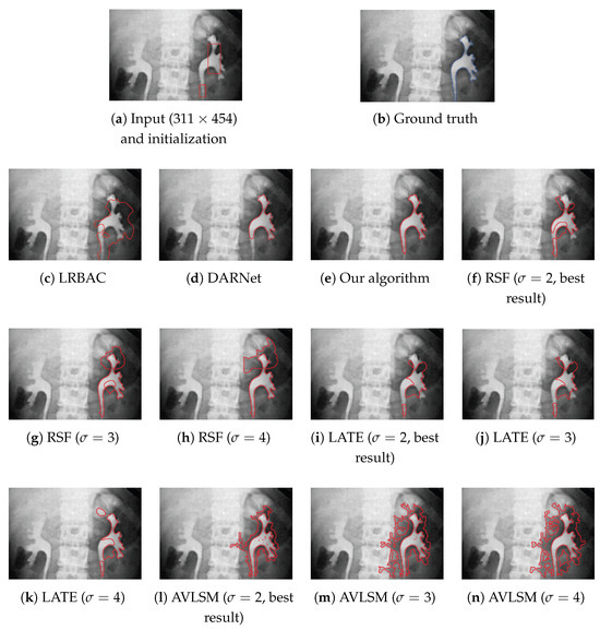
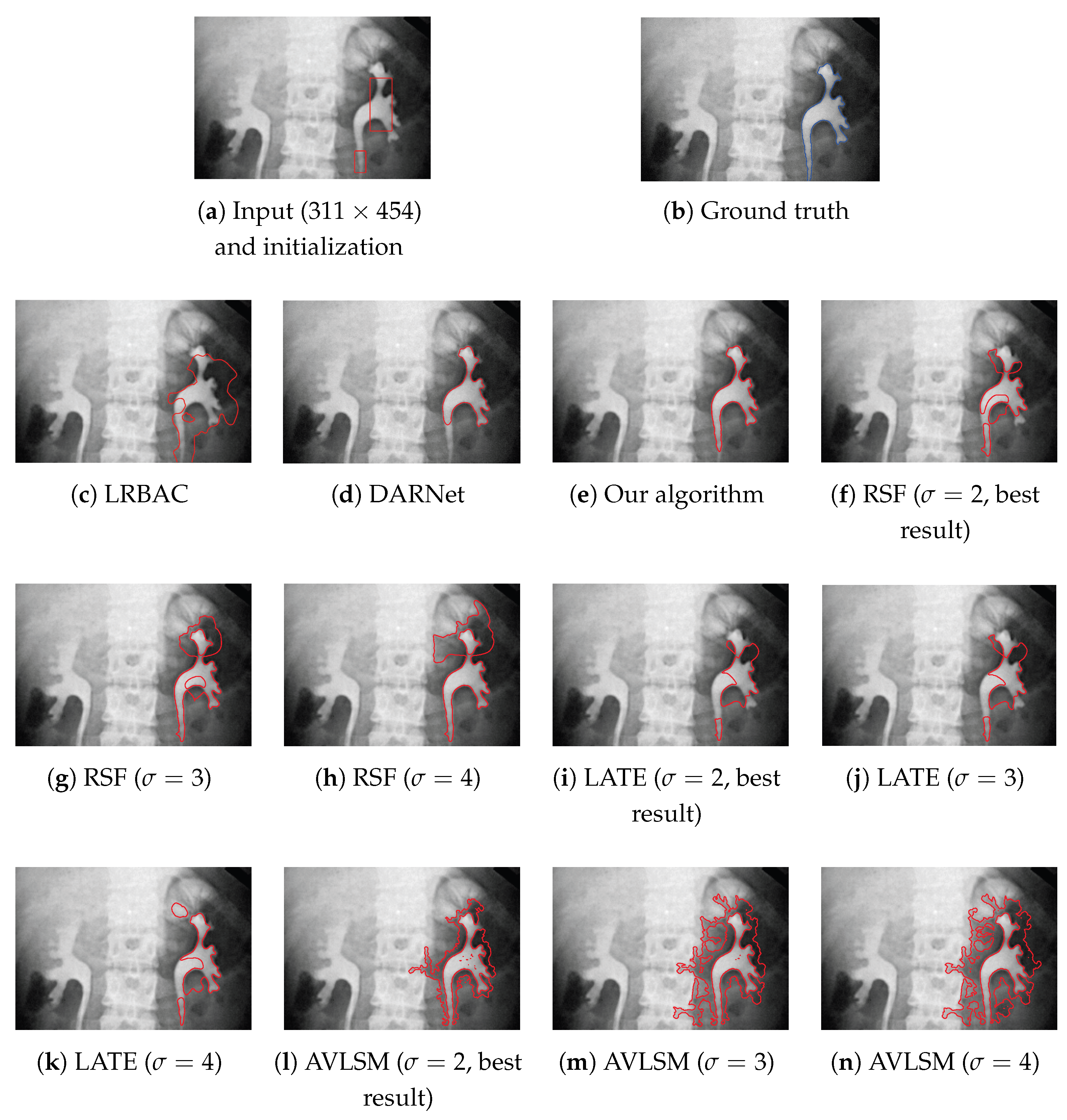
To rigorously evaluate the proficiency of our algorithm in managing uneven illuminations, we conduct a third experiment where we attempt to recover an kidney tube, as depicted in Figure 5. The image under test exhibits pronounced uneven illuminations, with particular intensity around the object’s vicinity. To address these challenges, we strategically place two initial curves as illustrated in Figure 5a. These curves are aimed at compensating for the uneven illuminations and the faint edges observable at the object’s base.
Figure 5.
Results of different algorithms on the recovery of one kidney tube: (a) the input image and the initial curve location, (b) the ground truth boundary of the object (identified by the blue curve), (c) the segmentation result given by LRBAC (terminated after 1000 iterations), (d) the result given by GARNet, (e) the result given by our algorithm, (f–h) different results given by RSF with different settings of , (i–k) different results given by LATE with different settings of , and (l–n) different results given by AVLSM with different settings of . For RSF, LATE, and AVLSM, the best results are measured by Dice.
Despite our efforts, the RSF, LATE, and AVLSM methods prove unsuccessful in object recovery, irrespective of the parameter settings. Specifically, for values of 2, 3, and 4, the active curve consistently fails to converge to the object boundary, leading to erroneous outcomes as shown in Figure 5f–n. The LRBAC method, once more, is unable to meet the challenge, as seen in Figure 5c. DARNet provides a relatively accurate result, but cannot recover more parts of the object boundary (Figure 5d). In contrast, our proposed snake algorithm emerges as the sole technique capable of segmenting the object, as demonstrated in Figure 5e. It is important to note, however, that while our method achieved segmentation, the result was not without imperfections.
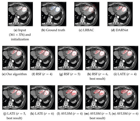
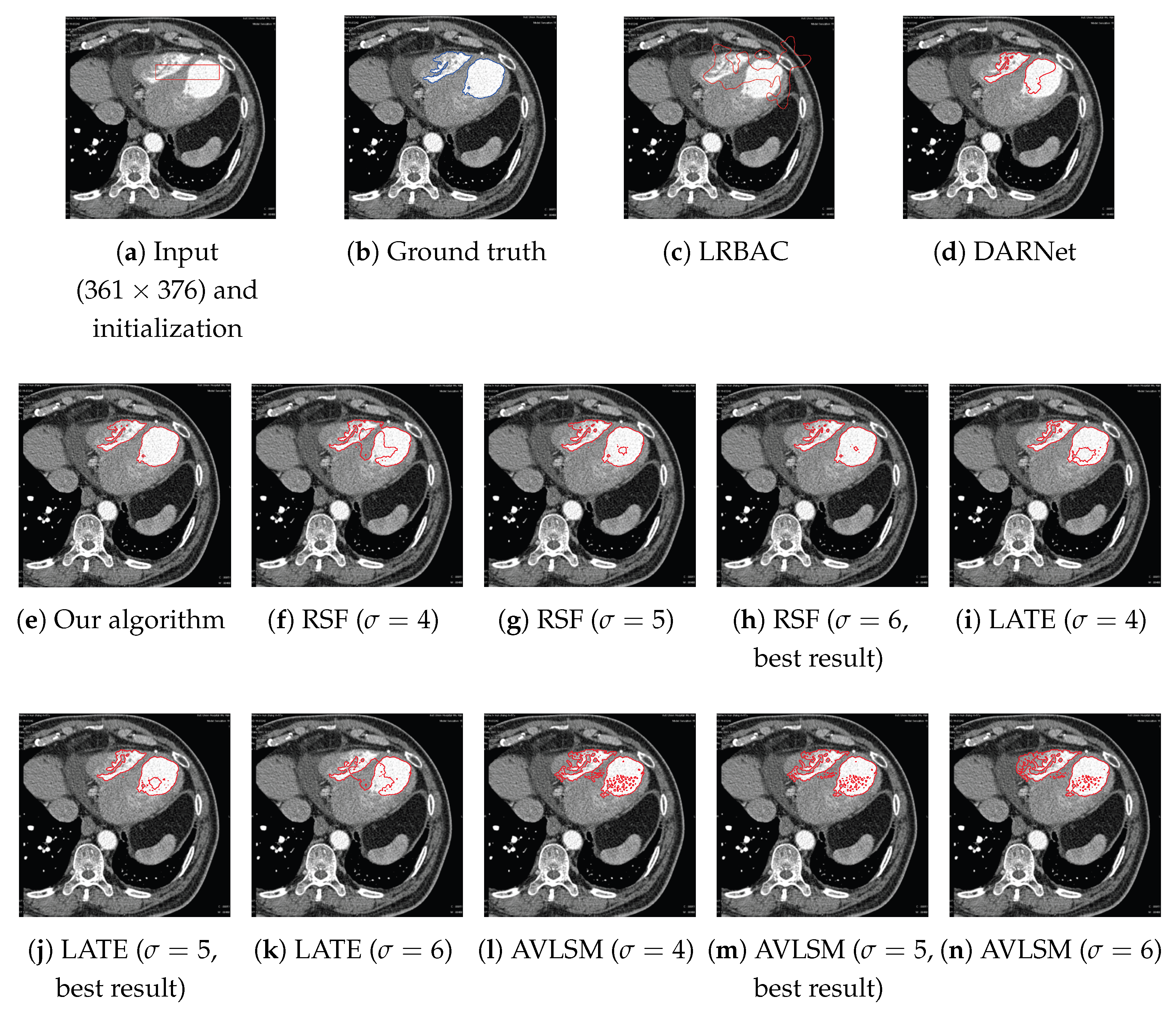
In our subsequent experiment, our primary objective is to reconstruct the ventricle from the test image, as depicted in Figure 6. The initialization process is demonstrated in Figure 6a. When comparing the outcomes achieved by the LRBAC, DARNet, RSF, LATE, AVLSM, and our proposed algorithm, we observed the following:
Figure 6.
Results of different algorithms on recovering the blood regions in the ventricle: (a) the input image and the initial curve location, (b) the ground truth boundary of the object (identified by the blue curve), (c) the segmentation result given by LRBAC (terminated after 1000 iterations), (d) the result given by GARNet, (e) the result given by our algorithm, (f–h) different results given by RSF with different settings of , (i–k) different results given by LATE with different settings of , and (l–n) different results given by AVLSM with different settings of . For RSF, LATE, and AVLSM, the best results are measured by Dice.
In order to quantitatively compare those segmentation results above, we use the Dice coefficient [62]
where GT denotes the ground truth object and MG denotes the object recovered by models. Table 1 shows the Dice coefficients, iterations, and computation times when different models complete the relative segmentation tasks given in Figure 3, Figure 4, Figure 5 and Figure 6. It is noted that for RSF, LATE, and AVLSM, we select those best results for comparison.
Table 1.
Quantitatively comparative results on four medical images.
Medical images primarily serve as the core subjects for parametric statistical snakes. However, these algorithms are versatile and can be applied to various images beyond medical imaging. To demonstrate the efficacy and adaptability of our proposed algorithm, we conducted two separate experiments focusing on the segmentation of regular optical images.
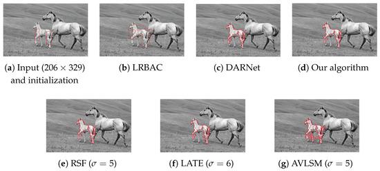
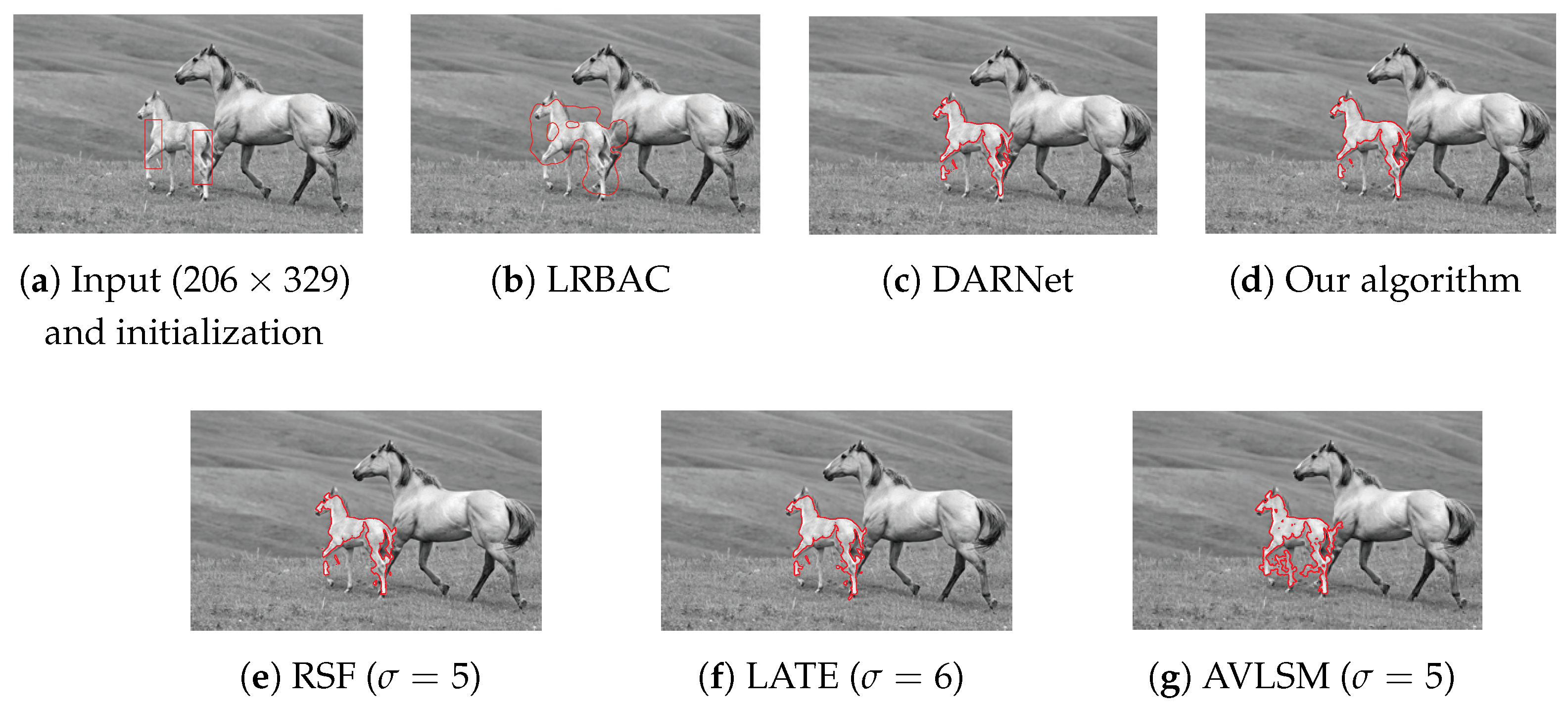
In the first experiment, we observe the segmentation performance on an image of a little horse. While the algorithms RSF and LATE can delineate most of the horse’s features as shown in Figure 7e,f, LRBAC consistently returns unsatisfactory results, as evidenced in Figure 7b. AVLSM recovers the most parts of the object compared with the other algorithms, but several leaked boundaries are presented (Figure 7g). Notably, DARNet and our proposed algorithm emerge as the most effective, accurately segmenting the little horse (Figure 7c,d).
Figure 7.
Results of different algorithms on the recovery of one horse: (a) the input image and the initial curve location, (b), the result given by LRBAC, (c) the result given by DARNet, (d) the result given by our algorithm, (e) the result given by RSF, (f) the result given by LATE, and (g) the result given by AVLSM.
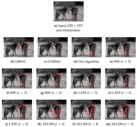
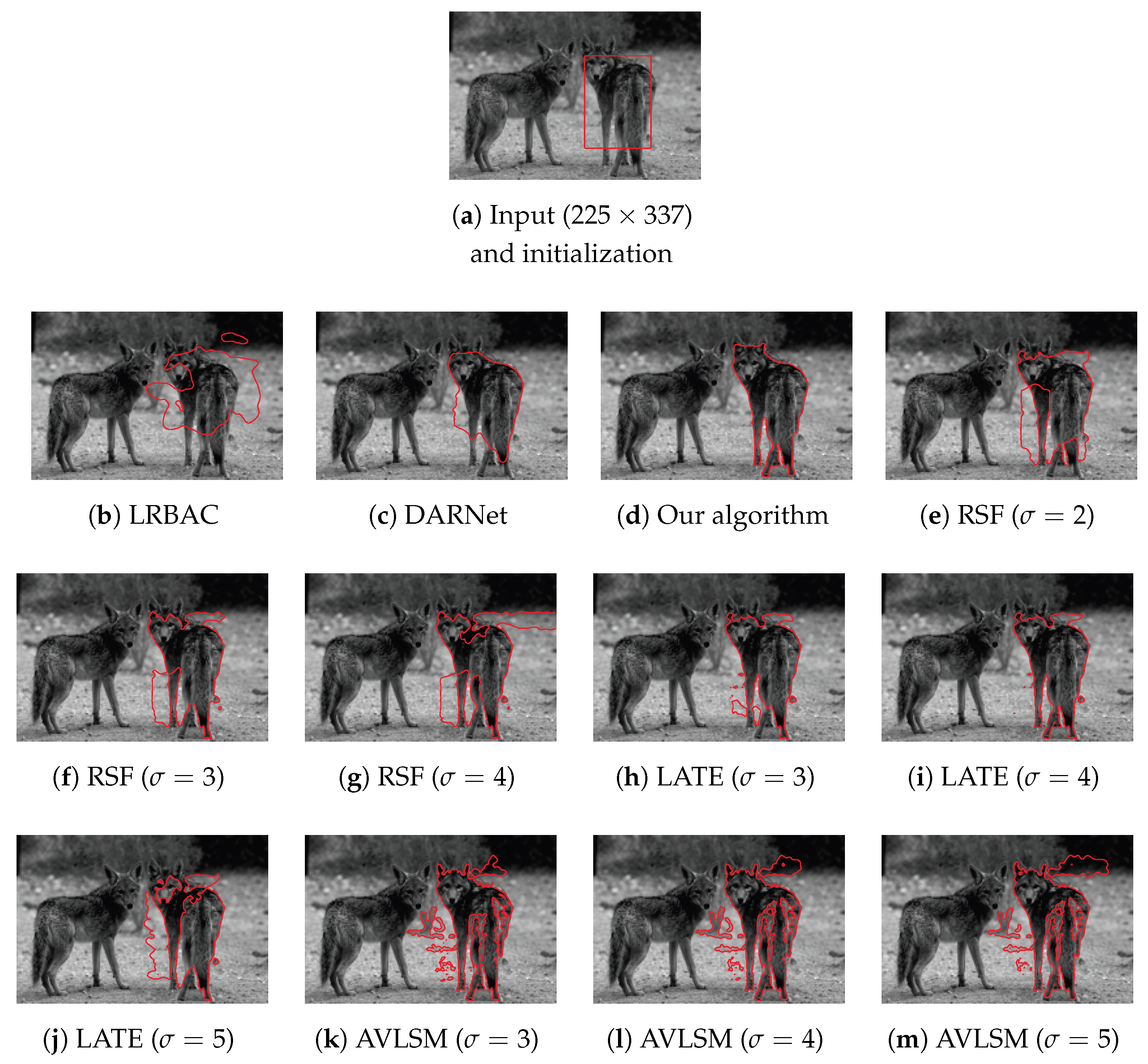
The second experiment is conducted on an image of a wolf. Interestingly, RSF, LATE, and AVLSM cannot achieve a satisfactory segmentation from Figure 8e–m, and LRBAC’s results are markedly off, as depicted in Figure 8b. DARNet gives an immature result (Figure 8c). Once again, our algorithm showcases its prowess by segmenting the wolf accurately and capturing the most precise boundary (Figure 8d).
Figure 8.
Results of different algorithms on the recovery of one wolf: (a) the input image and the initial curve location, (b), the result given by LRBAC, (c) the result given by DARNet, (d) the result given by our algorithm, (e–g) the results given by RSF with different settings, (h–j) the results given by LATE with different settings, and (k–m) the results given by AVLSM with different settings.
In summary, while other algorithms demonstrate varying efficiency, our proposed algorithm consistently outperforms them in both experimental setups, underscoring its potential for diverse imaging applications.
After this subsection, we would like to emphasize that in our proposed algorithm, the only two deviations from RSF’s computational routines are the data collection mode and the different dynamic kernel. This ensures that our algorithm remains computationally efficient, having a computational complexity on par with RSF. Compared with LATE and AVLSM, our proposed algorithm involves fewer terms and parameters, so its computational efficiency is higher than LATE and AVLSM (refer to Table 1).
4.2. Effects of and
The parameters and are pivotal in our proposed algorithm. Their values play a crucial role in defining the data collection scope. Their correct configuration ensures that the snake algorithm converges stably and precisely to the object boundaries. We present detailed evaluations using two test examples in this subsection to elucidate their significance.
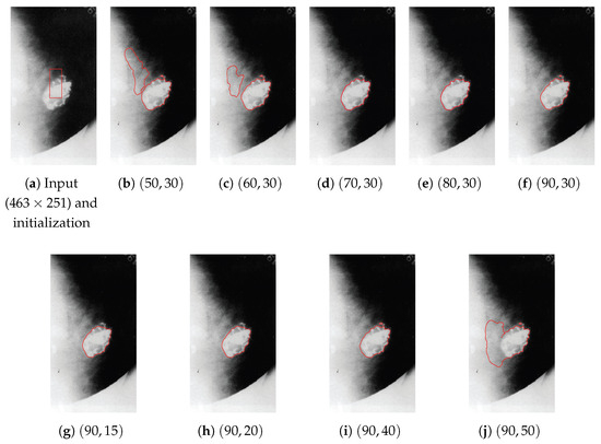
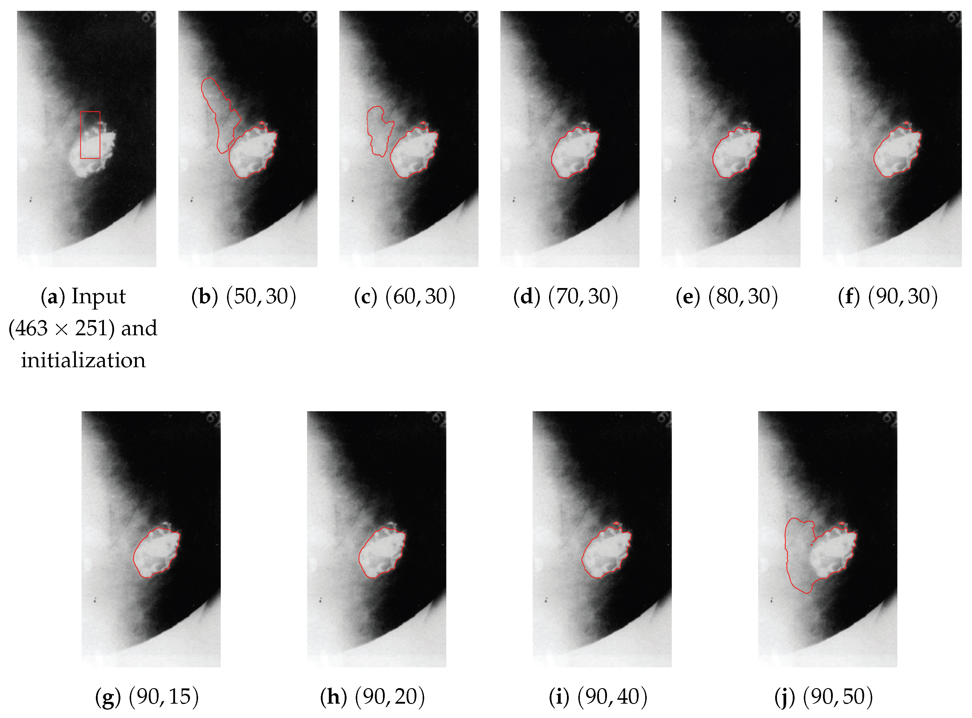
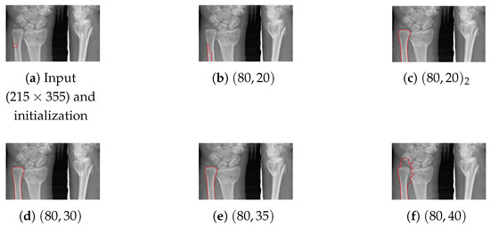
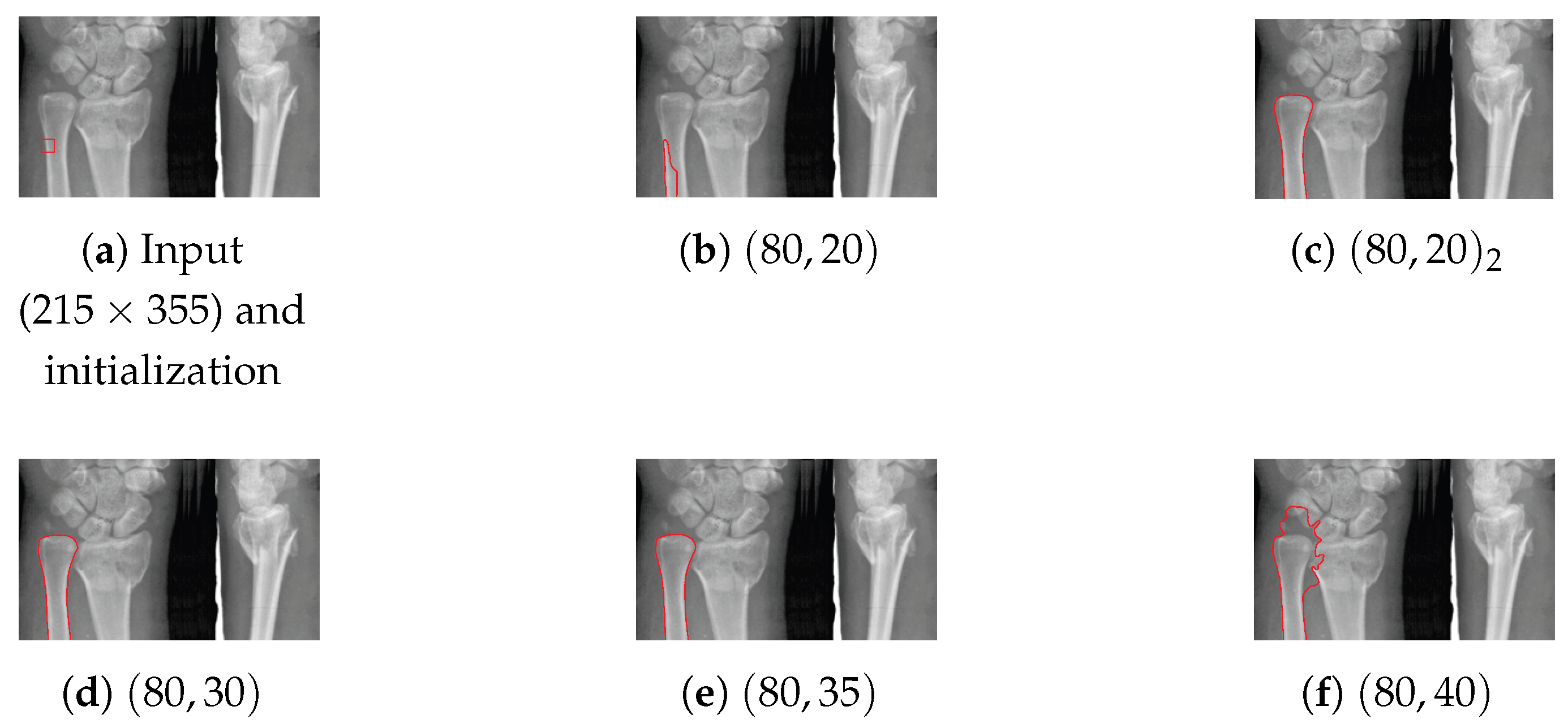
The first test involves an X-ray image characterized by pronouncedly uneven illuminations and a subtle edge on its left side, as depicted in Figure 9a. For this evaluation, we systematically varied the values of and to understand their influence on the segmentation process. The outcomes of these variations are documented in Figure 9.
Figure 9.
Results of our proposed algorithm on an X-ray image, with different and settings. In (b–j), .
A critical observation is that larger values of ensure the snake’s stable progression towards the object boundary, as evident from Figure 9d–i. In contrast, setting a diminutive value for tends to divert the snake away from the intended boundary, as illustrated by Figure 9b,c. Meanwhile, favoring smaller values of results in more precise outcomes (Figure 9d–i), whereas an increased can lead to boundary overspill, as shown in Figure 9j.
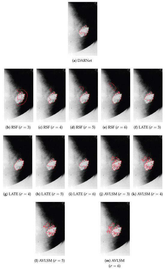
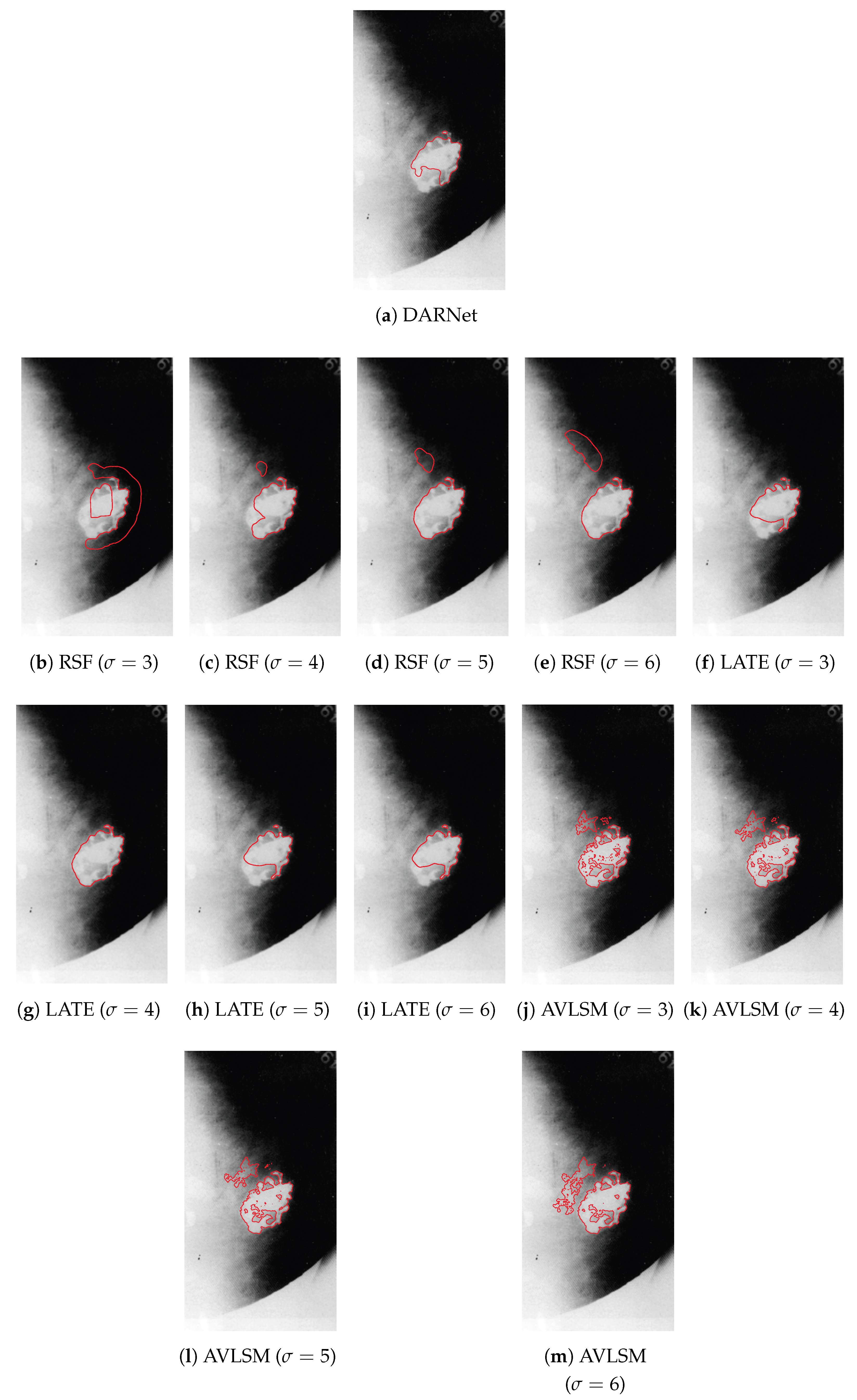
Through these experiments, we further observe the robustness of our proposed algorithm to variations in and . Specifically, for an initialization depicted in Figure 9a, even with varied settings such as and , the algorithm consistently delivers accurate results. It is worth mentioning that, under identical initialization conditions as in Figure 9a, DARNet, RSF, and AVLSM methods cannot yield results as precise as our snake, as seen in Figure 10. Only when can the LATE approach produce a comparable outcome. For alternative settings, LATE predominantly offered premature segmentation outcomes.
Figure 10.
Results of RSF, LATE and AVLSM on Figure 9a, with different settings. (a) The result given by DARNet, (b–e) results given by RSF with different settings, (f–i) results given by LATE with different settings, and (j–m) results given by AVLSM with different settings.
In a subsequent experiment, we endeavored to reconstruct a fragment of bone. The starting curve, intriguingly, is situated quite distant from the majority of the object’s edges, as depicted in Figure 11a. A comprehensive display of the experimental outcomes can be observed in Figure 11.
Figure 11.
Results of our algorithm on the recovery of a piece of bone, with different settings of . In (b–d), . In (c), we decrease r by 1 every 4 iterations.
A discerning observer will note that when is inappropriately minimized, the snake model falls short in executing the segmentation task effectively, as illustrated in Figure 11b. This shortcoming arises primarily because, as the value of r diminishes to , the snake has not yet progressed sufficiently towards encompassing the entire boundary of the object. As a result, the gathered regional data remains inadequate in directing the snake toward the precise boundary of the object.
One could initially consider enlarging the value of to address this challenge. However, a more optimal solution would be to extend the rate at which r decreases. Remarkably, by diminishing r by a unit after every four iterations, the snake eventually succeeds in its task, as showcased in Figure 11c.
It is also worth noting that by judiciously increasing to an appropriate magnitude, the snake invariably manages to encompass the object, a fact evident from Figure 11d,e. Yet caution must be exercised. When is excessively amplified, the snake tends to overshoot, moving beyond even faint edges, a phenomenon evident in Figure 11f.
A persistent challenge with active contour methodologies lies in asserting that a triumphant segmentation is predominantly contingent on judicious initialization. Regrettably, our proposed snake model is not immune to this predicament. In situations characterized by poor initialization, meticulous calibration of and becomes indispensable.
5. Conclusions and Discussion
In this study, we propose a new localized snake algorithm. By altering the foundational construction logic, our proposed algorithm rectifies the issues found in the LRBAC framework [52], specifically its poor convergence stability and its sensitivity to initial conditions. Based on this, we further present a way to dynamically adjust the data collection scope (i.e., localization size) of the snake. The dynamical localization size ensure both our methodology’s convergence stability and segmentation accuracy. In addition, since our proposed algorithm employs the simple first-order statistical moment, specifically the mean, it can be fast implemented using the convolution.
When contrasted with the state-of-the-art RSF [41] and other algorithms that draw inspiration from RSF, such as LATE and AVLSM, our algorithm leans more towards an edge-based paradigm. This is underscored by its unique mode of data collection. This unique feature enables our method to handle challenges like uneven illuminations and low contrasts with greater proficiency.
Experimental results from real-image segmentation further underscore the effectiveness and robustness of our proposed algorithm. Additionally, we furnish detailed derivations and computations for key equations featured in this paper for clarity and completeness.
From the experimental results of “kidney” (Figure 5), “horse” (Figure 7), and “wolf” (Figure 8), it can be seen that our proposed algorithm still has typical limitations in processing uneven illumination and low-contrast images. Involving more statistical moments [63], adding interaction terms, or integrating with popular Deep Learning techniques [57,58] to improve our algorithm’s segmentation accuracy, flexibility, and adaptability in various scenarios are our next research objectives. Finally, since this paper focuses on the basic theoretical analysis and the segmentation capability improved by the proposed algorithm, we adopt a proven and commonly used numerical implementation method to compute our algorithm (and the existing algorithms). The computation speed of the proposed algorithm currently cannot meet the requirements for real-time performance. In the future, it is interesting to borrow more advanced computational methods and techniques (such as the state-of-the-art Hamiltonian fast marching [32]) to improve the implementation speed and make the proposed algorithm more feasible for deployment in real-world settings.
Author Contributions
Conceptualization, M.Y.; methodology, M.Y.; formal analysis, Q.L.; writing—original draft, Q.L.; writing—review and editing, M.Y.; visualization, Q.L. All authors have read and agreed to the published version of the manuscript.
Funding
This work was supported by the National Natural Science Foundation of China (Grant No. 12571401), the Heilongjiang Provincial Natural Science Foundation Joint Guidance Project (No. JJ2024LH0820), and the Fundamental Research Funds for the Central Universities (No. 30722024CFJ2403).
Institutional Review Board Statement
All authors certify that this research does not involve human participants and/or animals. There is no potential conflict of interest with any organization and individual in this research.
Data Availability Statement
All data generated or analyzed during this study are included in this manuscript. The code written for this manuscript and the test figures are openly available in GitHub at https://github.com/yangming1984/A-Localized-Snake-with-Dynamic-Size (accessed on 7 September 2025). Further inquiries can be directed to the corresponding author.
Acknowledgments
The authors thank the reviewers for commenting and improving our manuscript.
Conflicts of Interest
All authors certify that they have no affiliations with or involvement in any organization or entity with any financial interest or non-financial interest in the subject matter or materials discussed in this manuscript.
Appendix A. Derivation of the Gradient Field of (47)
To compute the first variation of , consider a slight perturbation of , denoted as , where is a perturbation field satisfying the condition for all . Let be a small scalar in the interval (−1,1). Given this perturbation, the energy functional becomes
with
and
To evaluate the derivative of with respect to at , and applying the product rule, we find
First, we note that for the zero level set, the value of evaluates to zero. Given this, the expression for when and becomes
On further inspection, we can deduce the following:
Similarly, it can be obtained that
Combining the above, we obtain
By switching the order of integration:
Upon exchanging the variables of integration, we arrive at the following:
Finally, equating our results with Equation (A1), the gradient is expressed as
References
- Kass, M.; Witkin, A.; Terzopoulos, D. Snakes: Active contour models. Int. J. Comput. Vis. 1987, 1, 321–331. [Google Scholar] [CrossRef] [Scilit]
- Caselles, V.; Kimmel, R.; Sapiro, G. Geodesic active contours. Int. J. Comput. Vis. 1997, 22, 61–79. [Google Scholar] [CrossRef] [Scilit]
- Chan, T.F.; Vese, L. Active contours without edges. IEEE Trans. Image Process. 2001, 10, 266–277. [Google Scholar] [CrossRef] [Scilit]
- Ronfard, R. Region-based strategies for active contour models. Int. J. Comput. Vis. 1994, 13, 229–251. [Google Scholar] [CrossRef] [Scilit]
- Zhu, S.; Yuille, A. Region competition: Unifying snakes, region growing and Bayes/MDL for multiband image segmentation. IEEE Trans. Pattern Anal. Mach. Intell. 1996, 8, 884–900. [Google Scholar] [CrossRef] [Scilit]
- Li, C.; Huang, R.; Ding, Z.; Gatenby, J.C.; Metaxas, D.N.; Gore, J.C. A level set method for image segmentation in the presence of intensity inhomogeneities with application to MRI. IEEE Trans. Image Process. 2011, 20, 2007–2016. [Google Scholar] [CrossRef] [Scilit] [PubMed]
- Xu, C.; Prince, J.L. Snakes, shapes, and gradient vector flow. IEEE Trans. Image Process. 1998, 7, 359–369. [Google Scholar] [CrossRef] [Scilit]
- Xu, C.; Prince, J.L. Generalized gradient vector flow external forces for active contours. Signal Process. 1998, 71, 131–139. [Google Scholar] [CrossRef] [Scilit]
- Li, Q.; Deng, T.; Xie, W. Active contours driven by divergence of gradient vector flow. Signal Process. 2016, 120, 185–199. [Google Scholar] [CrossRef] [Scilit]
- Li, B.; Acton, S.T. Active contour external force using vector field convolution for image segmentation. IEEE Trans. Image Process. 2007, 16, 2096–2106. [Google Scholar] [CrossRef] [Scilit]
- Jalba, A.C.; Wilkinson, M.H.F.; Roerdink, J.B.T.M. CPM: A Deformable Model for Shape Recovery and Segmentation Based on Charged Particles. IEEE Trans. Pattern Anal. Mach. Intell. 2004, 26, 1320–1335. [Google Scholar] [CrossRef] [Scilit]
- Xie, X.; Mirmehdi, M. MAC: Magnetostatic active contour model. IEEE Trans. Pattern Anal. Mach. Intell. 2008, 30, 632–647. [Google Scholar] [CrossRef] [Scilit] [PubMed]
- Yeo, S.Y.; Xie, X.; Sazonov, I.; Nithiarasu, P. Geometrically induced force interaction for three-dimensional deformable models. IEEE Trans. Image Process. 2011, 20, 1373–1387. [Google Scholar]
- Li, C.; Liu, J.; Fox, M.D. Segmentation of external force field for automatic initialization and splitting of snakes. Pattern Recognit. 2005, 38, 1947–1960. [Google Scholar] [CrossRef] [Scilit]
- Ghosh, P.; Bertelli, L.; Sumengen, B.; Manjunath, B.S. A nonconservative flow field for robust variational image segmentation. IEEE Trans. Image Process. 2010, 19, 478–490. [Google Scholar] [CrossRef] [Scilit]
- Tao, W.; Tai, X. Multiple piecewise constant with geodesic active contours (MPC-GAC) framework for interactive image segmentation using graph cut optimization. Image Vis. Comput. 2011, 29, 499–508. [Google Scholar] [CrossRef] [Scilit]
- Gao, X.; Wang, B.; Tao, D.; Li, X. A relay level set method for automatic image segmentation. IEEE Trans. Syst. Man Cybern. 2011, 41, 518–525. [Google Scholar]
- Malladi, R.; Sethian, J.A.; Vemuri, B.C. Shape modeling with front propagation: A level set approach. IEEE Trans. Pattern Anal. Mach. Intell. 1995, 17, 158–175. [Google Scholar] [CrossRef] [Scilit]
- Kim, J.; Fisher, J.; Yezzi, A.; Cetin, M.; Willsky, A. A nonparametric statistical method for image segmentation using information theory and curve evolution. IEEE Trans. Image Process. 2005, 14, 1486–1502. [Google Scholar]
- Michaelovich, O.; Rathi, Y.; Tannenbaum, A. Image segmentation using active contours driven by the Bhattacharyya gradient flow. IEEE Trans. Image Process. 2007, 16, 2787–2801. [Google Scholar] [CrossRef] [Scilit] [PubMed]
- Wu, H.; Appia, V.; Yezzi, A. Numerical conditioning problems and solutions for nonparametric i.i.d. statistical active contours. IEEE Trans. Pattern Anal. Mach. Intell. 2013, 35, 1298–1311. [Google Scholar] [CrossRef] [Scilit]
- Li, Q.; Deng, T. A nonparametric statistical snake model using the gradient flow of minimum probability density integration. J. Math. Imaging Vis. 2018, 60, 1150–1166. [Google Scholar] [CrossRef] [Scilit]
- Ni, K.; Bresson, X.; Chan, T.; Esedoglu, S. Local histogram based segmentation using the Wasserstein Distance. Int. J. Comput. Vis. 2019, 84, 97–111. [Google Scholar] [CrossRef] [Scilit]
- Sundaramoorthi, G.; Yezzi, A.; Mennucci, A.C. Sobolev active contours. Int. J. Comput. Vis. 2007, 73, 345–366. [Google Scholar] [CrossRef] [Scilit]
- Li, H.; Yezzi, A. Local or global minima: Flexible dual-front active contours. IEEE Trans. Pattern Anal. Mach. Intell. 2007, 29, 1–14. [Google Scholar] [CrossRef] [Scilit] [PubMed]
- Mishra, A.K.; Fieguth, P.W.; Clausi, D.A. Decoupled active contour (DAC) for boundary detection. IEEE Trans. Pattern Anal. Mach. Intell. 2011, 33, 310–324. [Google Scholar] [CrossRef] [Scilit]
- Bal, S.S.; Chen, K.; Yang, F.P.G.; Peng, G.S. Arterial input function segmentation based on a contour geodesic model for tissue at risk identification in ischemic stroke. Med. Phys. 2022, 49, 2475–2485. [Google Scholar] [CrossRef] [Scilit]
- Gorelick, L.; Veksler, O.; Boykov, Y.; Nieuwenhuis, C. Convexity shape prior for binary segmentation. IEEE Trans. Pattern Anal. Mach. Intell. 2017, 39, 258–271. [Google Scholar] [CrossRef] [Scilit]
- Gulshan, V.; Rother, C.; Criminisi, A.; Blake, A.; Zisserman, A. Geodesic star convexity for interactive image segmentation. In Proceedings of the 2010 IEEE Computer Society Conference on Computer Vision and Pattern Recognition; IEEE: Piscataway, NJ, USA, 2010; pp. 3129–3136. [Google Scholar]
- Shi, X.; Li, C. Convexity preserving level set for left ventricle segmentation. Magn. Reson. Imaging 2021, 78, 109–118. [Google Scholar] [CrossRef] [Scilit] [PubMed]
- Yan, S.; Tai, X.-C.; Liu, J.; Huang, H.-Y. Convexity shape prior for level set-based image segmentation method. IEEE Trans. Image Process. 2020, 29, 7141–7152. [Google Scholar] [CrossRef] [Scilit]
- Chen, D.; Mirebeau, J.-M.; Shu, M.-L.; Tai, X.-C.; Cohen, L. Geodesic models with convexity shape prior. IEEE Trans. Pattern Anal. Mach. Intell. 2023, 45, 8433–8452. [Google Scholar] [CrossRef] [Scilit]
- Paragios, N.; Deriche, R. Geodesic active regions: A new framework to deal with frame partition problems in computer vision. J. Vis. Commun. Image Represent. 2002, 13, 249–268. [Google Scholar] [CrossRef] [Scilit]
- Paragios, N.; Deriche, R. Geodesic active regions and level set methods for motion estimation and tracking. Comput. Vis. Image Underst. 2005, 97, 259–282. [Google Scholar] [CrossRef] [Scilit]
- Kimmel, R. Fast Edge Integration. In Geometric Level Set Methods in Imaging, Vision and Graphics; Osher, S., Paragios, N., Eds.; Springer: Berlin/Heidelberg, Germany, 2003. [Google Scholar]
- Chakraborty, A.; Staib, H.; Duncan, J. Deformable boundary finding in medical images by integrating gradient and region information. IEEE Trans. Med. Imaging 1996, 15, 859–870. [Google Scholar] [CrossRef]
- Haddon, J.; Boyce, J. Image segmentation by unifying region and boundary information. IEEE Trans. Pattern Anal. Mach. Intell. 1990, 12, 929–948. [Google Scholar] [CrossRef] [Scilit]
- Wang, B.; Gao, X.; Tao, D.; Li, X. A nonlinear adaptive level set for image segmentation. IEEE Trans. Cybern. 2014, 44, 418–428. [Google Scholar] [CrossRef] [Scilit]
- Chen, D.; Spencer, J.; Mirebeau, J.M.; Chen, K.; Shu, M.; Cohen, L.D. A generalized asymmetric dual-front model for active contours and image segmentation. IEEE Trans. Image Process. 2021, 30, 5056–5071. [Google Scholar] [CrossRef] [Scilit] [PubMed]
- Zhang, W.; Wang, X.; Chen, J.; You, W. A New Hybrid Level Set Approach. IEEE Trans. Image Process. 2020, 29, 7032–7044. [Google Scholar] [CrossRef] [Scilit]
- Li, C.; Kao, C.; Gore, J.C.; Ding, Z. Minimization of region-scalable fitting energy for image segmentation. IEEE Trans. Image Process. 2008, 17, 1940–1949. [Google Scholar] [CrossRef] [Scilit]
- Zhang, K.; Zhang, L.; Lam, K.; Zhang, D. A level set approach to image segmentation with intensity inhomogeneity. IEEE Trans. Cybern. 2016, 46, 546–557. [Google Scholar] [CrossRef] [Scilit]
- Min, H.; Jia, W.; Zhao, Y.; Zuo, W.; Ling, H.; Luo, Y. LATE: A level-set method based on local approximation of Taylor expansion for segmenting intensity inhomogeneous images. IEEE Trans. Image Process. 2018, 27, 5016–5031. [Google Scholar] [CrossRef] [Scilit]
- Cai, Q.; Liu, H.; Zhou, S.; Sun, J.; Li, J. An adaptive-scale active contour model for inhomogeneous image segmentation and bias field estimation. Pattern Recognit. 2018, 82, 79–93. [Google Scholar] [CrossRef] [Scilit]
- Li, M.; Li, B. A novel active contour model for noisy image segmentation based on adaptive fractional order differentiation. IEEE Trans. Image Process. 2020, 29, 9520–9531. [Google Scholar] [CrossRef] [Scilit]
- Wang, X.; Min, H.; Zhang, Y. Multi-scale local region based level set method for image segmentation in the presence of intensity inhomogeneity. Neurocomputing 2015, 151, 1086–1098. [Google Scholar] [CrossRef] [Scilit]
- Cai, Q.; Qian, Y.; Li, J.; Yang, Y.; Wu, F.; Zhang, D. AVLSM: Adaptive variational level set model for image segmentation in the presence of severe intensity inhomogeneity and high noise. IEEE Trans. Image Process. 2022, 31, 43–57. [Google Scholar] [CrossRef] [Scilit] [PubMed]
- Darolti, C.; Mertins, A.; Bodensteiner, C.; Hofmann, U. Local region descriptors for active contours evolution. IEEE Trans. Image Process. 2008, 17, 2275–2288. [Google Scholar] [CrossRef] [Scilit]
- Sundaramoorthi, G.; Soatto, S.; Yezzi, A. Curious snakes: A minimum latency solution to the cluttered background problem in active contours. In Proceedings of the 2010 IEEE Computer Society Conference on Computer Vision and Pattern Recognition; IEEE: Piscataway, NJ, USA, 2010; pp. 2855–2863. [Google Scholar]
- Wang, X.; Min, H.; Zou, L.; Zhang, Y. A novel level set method for image segmentation by incorporating local statistical analysis and global similarity measurement. Pattern Recognit. 2015, 48, 189–204. [Google Scholar] [CrossRef] [Scilit]
- Song, Y.; Peng, G.; Sun, D.; Xie, X. Active contours driven by Gaussian function and adaptive-scale local correntropy-based K-means clustering for fast image segmentation. Signal Process. 2020, 174, 107625. [Google Scholar] [CrossRef] [Scilit]
- Lankton, S.; Tannenbaum, A. Localizing region-based active contours. IEEE Trans. Image Process. 2008, 17, 2029–2039. [Google Scholar] [CrossRef] [Scilit]
- He, K.-M.; Gkioxari, G.; Dollar, P.; Girshick, R. Mask R-CNN. In Proceedings of IEEE International Conference on Computer Vision; IEEE: Piscataway, NJ, USA, 2017; pp. 2980–2988. [Google Scholar]
- Shelhamer, E.; Long, J.; Darrell, T. Fully convolutional networks for semantic segmentation. IEEE Trans. Pattern Anal. Mach. Intell. 2017, 30, 640–651. [Google Scholar] [CrossRef] [Scilit] [PubMed]
- Girshick, R.; Donahue, J.; Darrell, T.; Malik, J. Region-based convolutional networks for accurate object detection and segmentation. IEEE Trans. Pattern Anal. Mach. Intell. 2016, 38, 142–158. [Google Scholar] [CrossRef] [Scilit]
- Ding, X.-F.; Zeng, T.-Y.; Tang, J.; Che, Z.-P.; Peng, Y.-X. A semantic representation refinement network for image segmentation. IEEE Trans. Multimed. 2022, 25, 5720–5732. [Google Scholar] [CrossRef] [Scilit]
- Cheng, D.; Liao, R.; Fidler, S.; Urtasun, R. DARNet: Deep Active Ray Network for Building Segmentation. In Proceedings of the IEEE/CVF Conference on Computer Vision and Pattern Recognition (CVPR); IEEE: Piscataway, NJ, USA, 2019; pp. 7423–7431. [Google Scholar]
- Le, N.; Quach, K.; Luu, K.; Savvides, M.; Zhu, C. Reformulating Level Sets as Deep Recurrent Neural Network Approach to Semantic Segmentation. arXiv 2017, arXiv:1704.03593. [Google Scholar] [CrossRef] [Scilit]
- Osher, S.; Sethian, J. Fronts propagating with curvature-dependent speed: Algorithms based on Hamilton-Jacobi formulations. J. Comput. Phys. 1988, 79, 12–49. [Google Scholar] [CrossRef] [Scilit]
- Yezzi, J.A.; Tsai, A.; Willsky, A. A fully global approach to image segmentation via coupled curve evolution equations. J. Vis. Comm. Image Rep. 2002, 13, 195–216. [Google Scholar] [CrossRef] [Scilit]
- Li, C.; Xu, C.; Gui, C.; Fox, M.D. Distance regularized level set evolution and its application to image segmentation. IEEE Trans. Image Process. 2010, 19, 3243–3254. [Google Scholar] [CrossRef] [Scilit] [PubMed]
- Zijdenbos, A.P. MRI Segmentation and the Quantification of White Matter Lesions. Ph.D. Thesis, Vanderbilt University Electrical Engineering Department, Nashville, TN, USA, 1994. [Google Scholar]
- Pang, Z.; Guan, Z.; Li, Y.; Chen, K.; Ge, H. Image Segmentation Based on the Hybrid Bias Field Correction. Appl. Math. Comput. 2023, 452, 128050. [Google Scholar] [CrossRef] [Scilit]

Disclaimer/Publisher’s Note: The statements, opinions and data contained in all publications are solely those of the individual author(s) and contributor(s) and not of MDPI and/or the editor(s). MDPI and/or the editor(s) disclaim responsibility for any injury to people or property resulting from any ideas, methods, instructions or products referred to in the content. |
© 2026 by the authors. Licensee MDPI, Basel, Switzerland. This article is an open access article distributed under the terms and conditions of the Creative Commons Attribution (CC BY) license.