An Explainable Artificial Intelligence Algorithm for Optimal Decision Making from a Business Analytics Perspective

Abstract

A feedforward neural network (FFNN) can effectively identify key factors that influence production system performance, which supports better decisions and cost reduction. This study utilizes an FFNN to compare the cost performance of two inventory approaches: fixed-time and fixed-size lots. The proposed algorithm has three artificial neurons representing three possible outcomes: fixed-size lots perform better, fixed-time lots perform better, and no significant difference in cost. The trained network’s parameters assess the importance of input to predict these outcomes. Moreover, an explainable artificial intelligence algorithm, called Shapley additive explanations (SHAP), is employed to explain FFNN outcomes. Moreover, two inventory conditions are included: lost sales and backordering. The analysis reveals that the key drivers of a lost-sales policy are modular availability and the degree of demand variability. Under the backordering strategy, demand variability, inventory holding cost, and stand-alone availability exert the strongest influence. The outcomes showed that fixed-size lots support a just-in-time approach when demand flexibility is low while there is high modular availability. However, when demand becomes more volatile and modular availability declines, results show that fixed-time lots provide a more cost-efficient alternative. These findings offer practical guidance for production control decisions, especially in high-volume discrete manufacturing settings such as automotive stamping operations.

1. Introduction

Machine learning algorithms are among the most robust techniques for inventory optimization (e.g., demand forecasting) [1]. Feedforward neural networks (FFNNs) are robust analytical tools for modeling nonlinear relationships between input variables and system outcomes in production environments. Batch manufacturing systems are affected by multiple interacting factors, including demand variability, inventory costs, machine availability, and operational policies, all of which influence cost efficiency and sustainability. Conventional analytical methods often fail to accurately capture these nonlinear interactions. An FFNN can overcome this limitation by learning from historical data and reliably predicting categorical or continuous outcomes. During backpropagation training, an FFNN learns to detect patterns and determine the relative importance of input factors. This allows managers to understand which variables most strongly affect production efficiency and cost performance. Applying a feedforward neural architecture to production systems supports better operational decisions, such as determining optimal batch sizes and reorder points, and selecting between the fixed-time lot strategy and the fixed-size policy. It also improves responsiveness to variability, reduces excess inventory, and lowers costs. Thus, it is valuable for gaining competitive advantages in complex manufacturing settings.

Systems that produce discrete items in large batches, such as those used in automotive sheet-metal stamping, exhibit substantial operational complexity, and their management directly influences overall cost performance. Workstations in these systems typically produce either fixed-time lots or fixed-size (quantity) lots [2]. In practice, workstations often experience random disruptions. These interruptions create variability in production duration for fixed-size lots, potentially delaying lot completion and affecting subsequent batches. In contrast, fixed-time lot systems maintain scheduled production duration despite disruptions. Instead, variability appears in the quantity produced within the allocated time.

Very little in-depth analytical work has been conducted—especially studies applying machine-learning techniques such as feed-forward neural networks—to explore how critical input variables influence cost outcomes in manufacturing environments. Literature mainly used traditional analytical methods (e.g., ANOVA) to find important components affecting system performance. However, these studies did not fully explore nonlinear relationships or explain how individual factors contribute to outcomes. This gap creates an opportunity for ML methods to provide a deeper analytical understanding for optimizing batch production decisions. Therefore, the research question in this study is: What are the key predictors of production systems?

To investigate this issue, a feedforward neural network is employed to uncover intricate relationships between system inputs and outputs. The approach captures underlying patterns and mathematical associations among multiple input variables and their respective settings across two manufacturing configurations—fixed-cycle batches and fixed-quantity batches. Insights generated by the network’s output layer enhance the interpretation of cost behavior and clarify the underlying cost dynamics in both batch-based production modes.

Therefore, the main contribution of this paper is its novel use of neural networks (NNs) to uncover functional relationships and identify critical factors affecting cost performance in fixed-time lot and fixed-size lot systems. Previous studies are limited in their capabilities to detect complex nonlinear interactions among multiple input factors. This paper addresses this gap and sheds light on how individual factors, including inventory holding costs, demand coefficient of variation, and stand-alone availability, affect system performance under lost sales and backordering policies. Additionally, this paper introduces a novel connection weight approach to quantitatively rank the relative importance of each input factor and to clarify their direct or inverse relationships with cost outcomes. This study contributes to the theory and practice by providing a robust analytical framework that advances decision-making in complex manufacturing environments. This approach enables production managers to strategically select and optimize production control systems, helping them reduce operational variability, improve responsiveness, and achieve significant cost savings.

The main contributions of this paper can be summarized as follows:

▪

A novel application of feedforward neural networks with the connection weight approach to quantify the relative importance of input factors in batch production systems.

▪

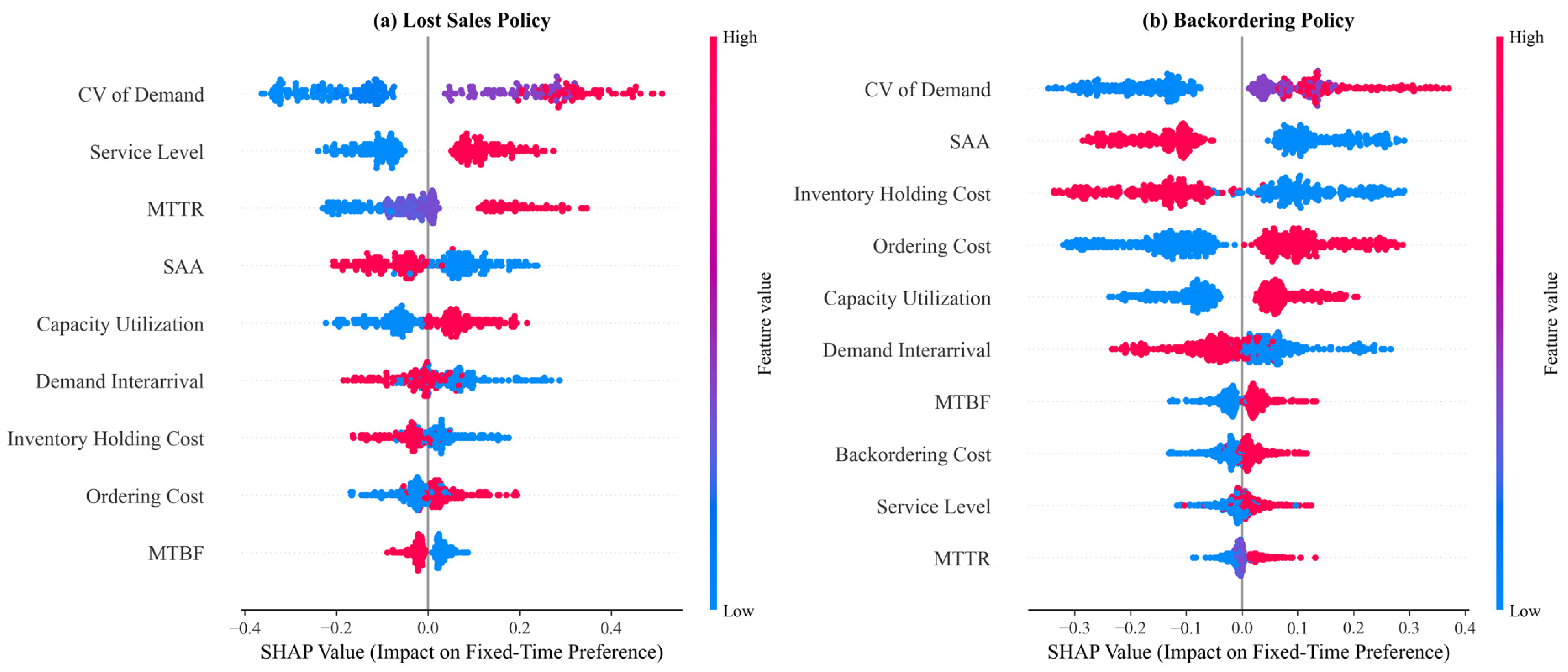
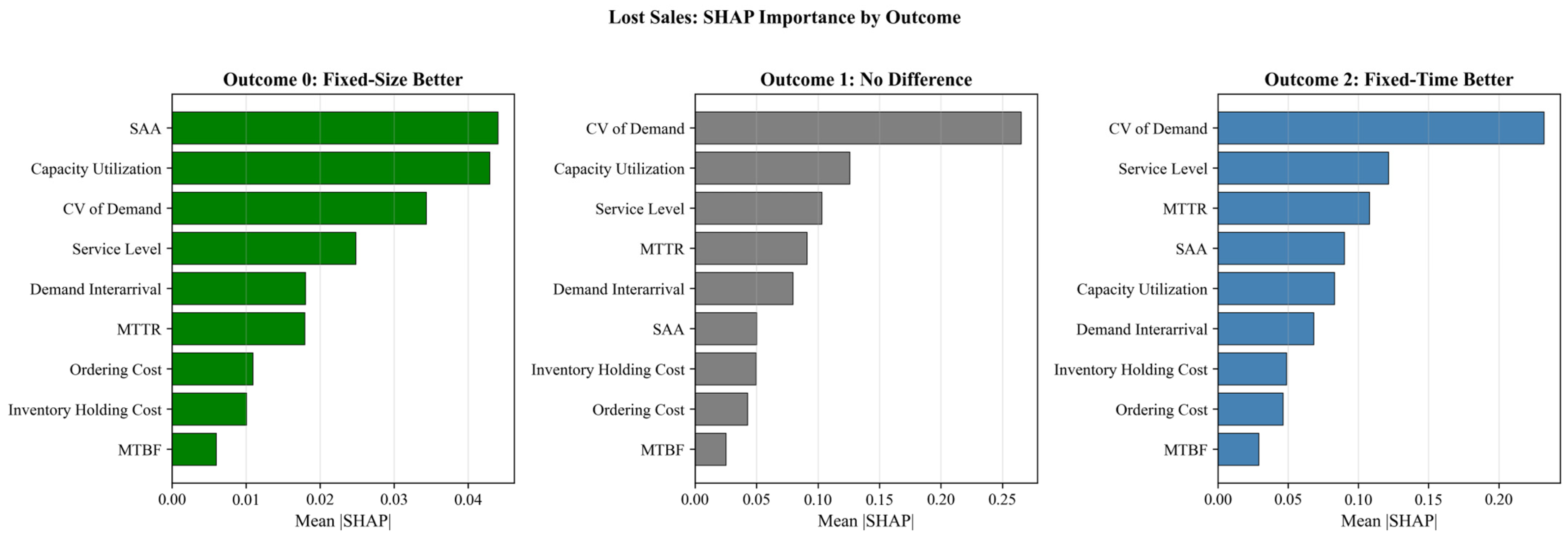
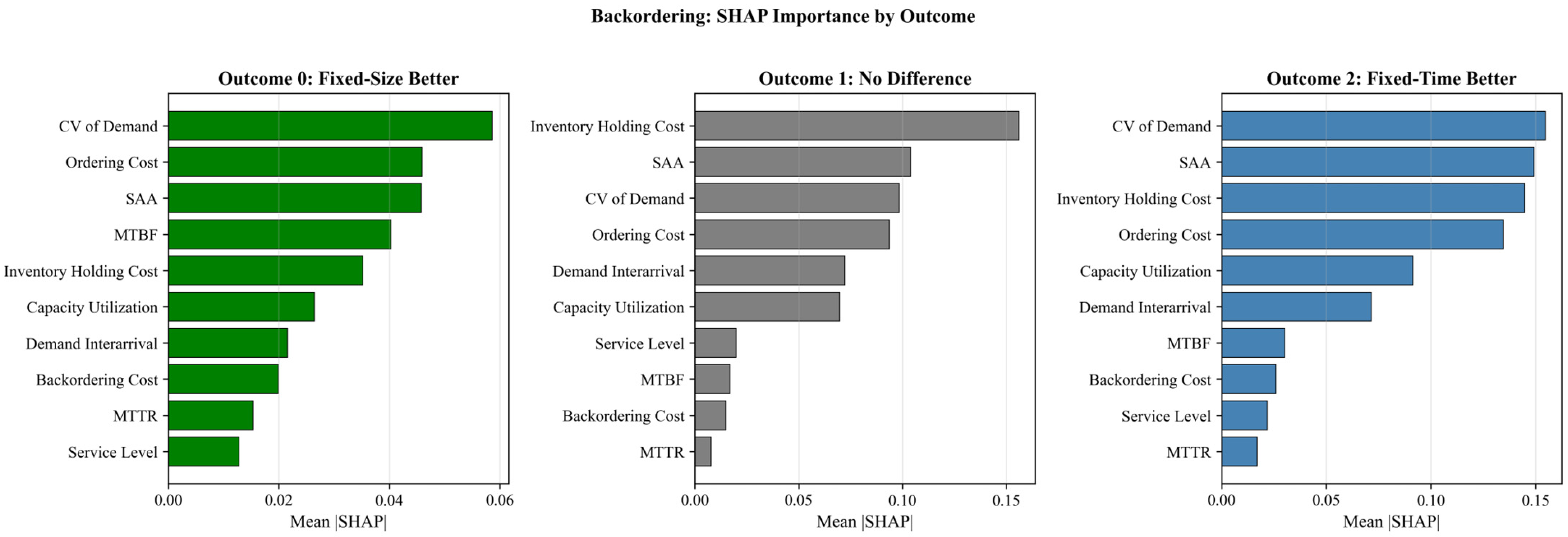
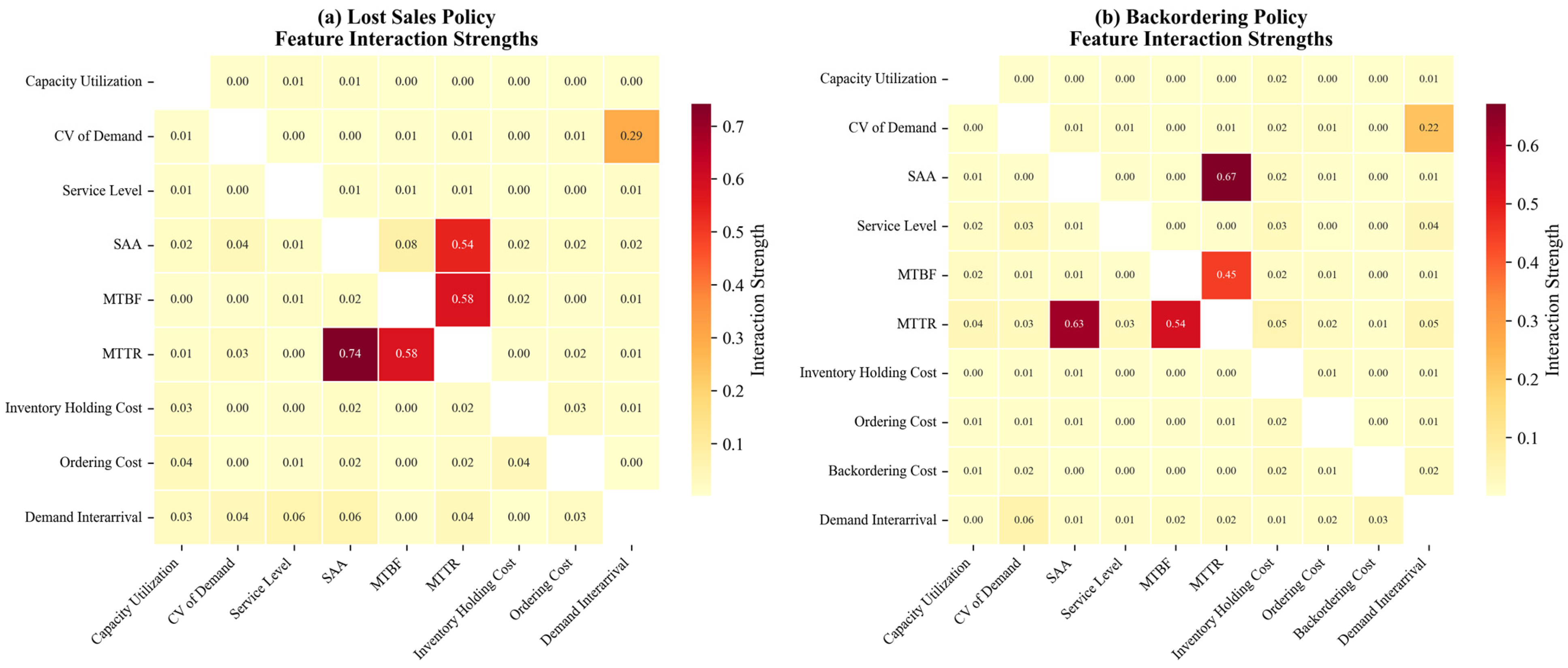
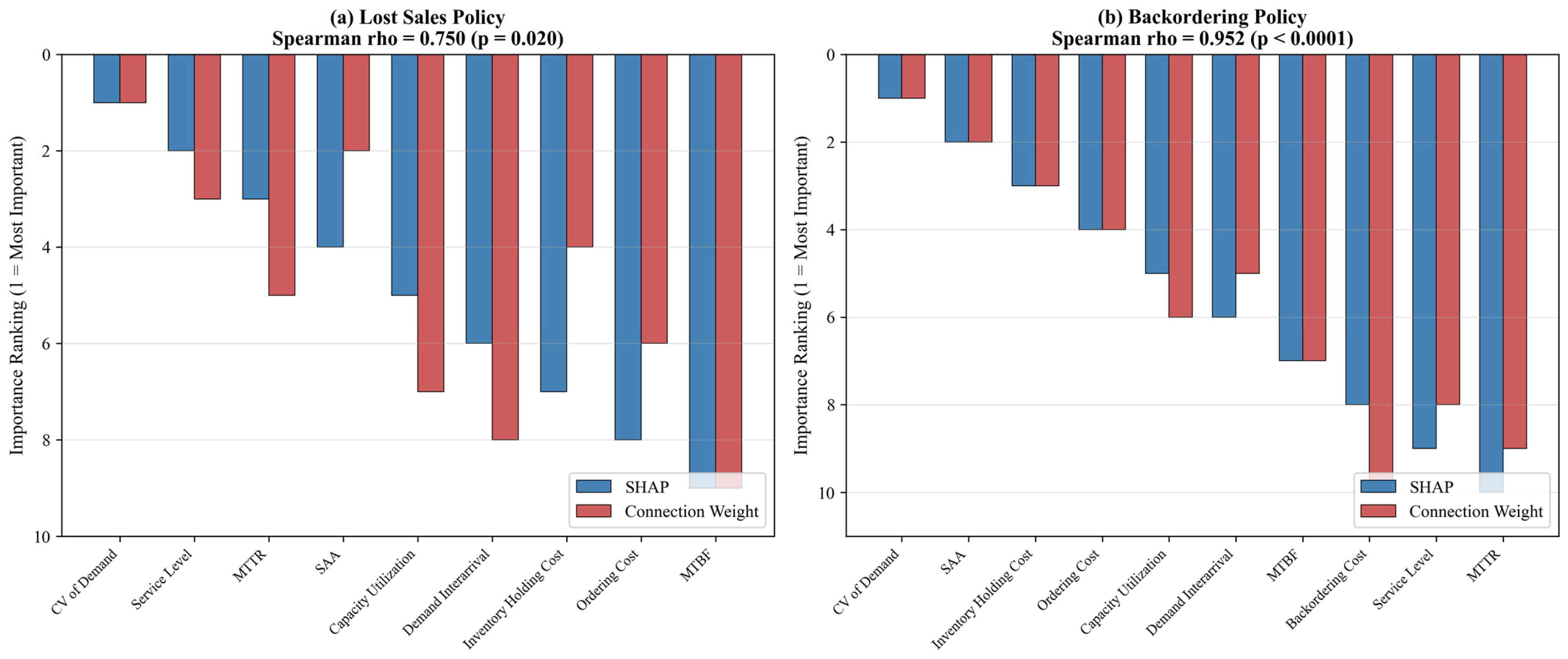
SHAP analysis to validate feature importance rankings and reveal non-linear relationships, with strong convergent validity between methods (Spearman ρ = 0.75–0.95).

▪

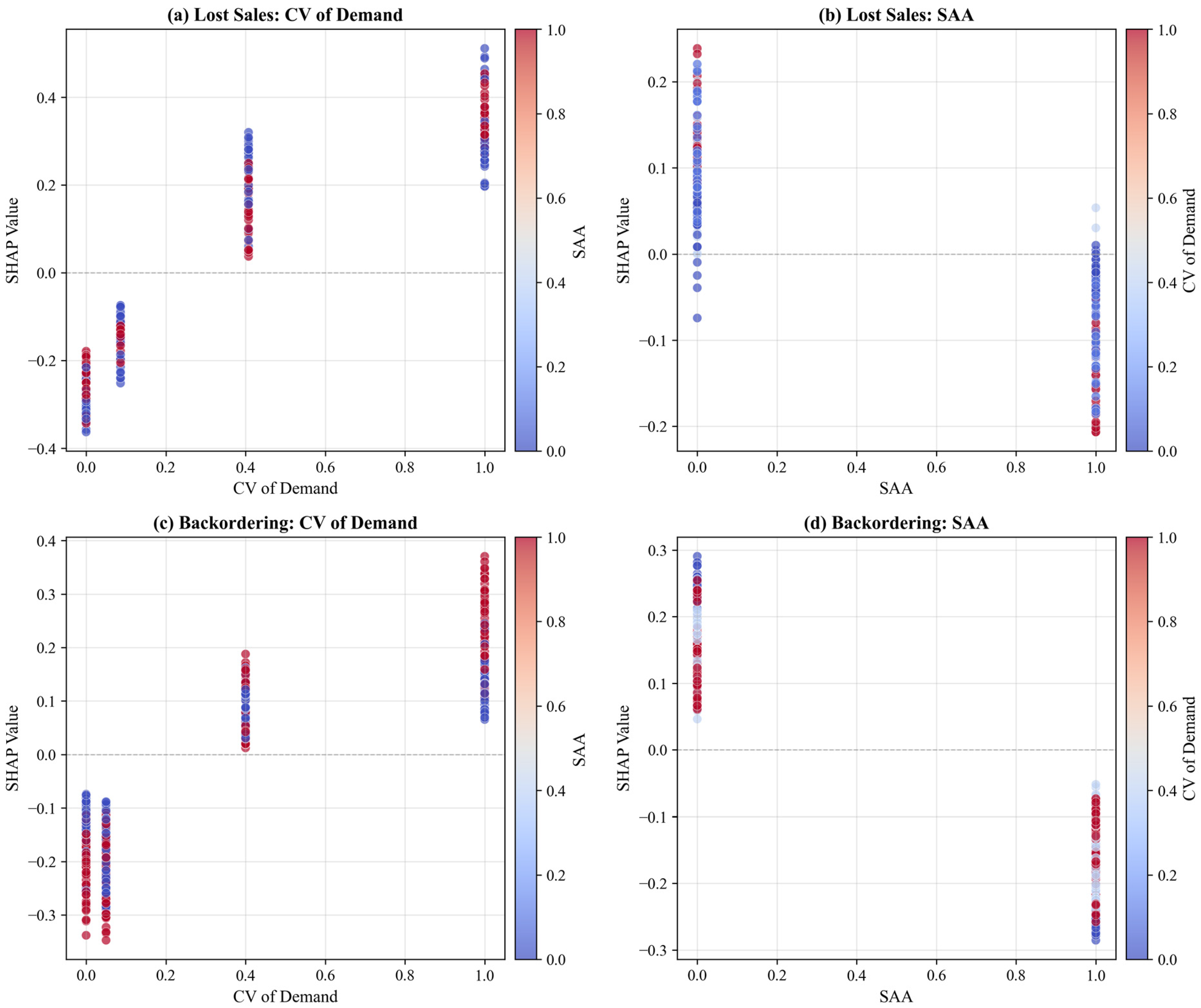
Identification of demand variability (CV of demand) and stand-alone availability (SAA) as the dominant factors influencing lot policy selection under both lost sales and backordering conditions.

▪

Discovery of a critical ~85% SAA threshold below which fixed-time lots consistently outperform fixed-size lots.

▪

Practical guidance for production managers to select optimal batch policies based on operational parameters.

The remainder of this paper is organized as follows. Section 2 reviews the relevant literature on batch production systems and neural network applications. Section 3 describes the data, neural network architecture, connection weight approach, and SHAP methodology. Section 4 presents results for both lost sales and backordering policies, including SHAP-based validation. Section 5 discusses managerial implications and limitations. Section 6 concludes the paper.

2. Literature Review

Extensive research has investigated batch production systems utilizing fixed-size lots under continuous review inventory policies. The primary focus of these studies has been on determining optimal lot sizes and reorder points to minimize total operational costs, including ordering, inventory holding, and costs associated with backordering or lost sales. Prominent contributions in this area include works by Federgruen and Zheng [3], who proposed efficient algorithms for continuous review systems. Similarly, Moon and Choi [4] and Parlar [5] provided valuable insights into managing inventory under varying service-level constraints and random supply interruptions. Mohebbi [6] further analyzed the impact of random lead times on lost-sales inventory systems, offering improved managerial strategies to cope with uncertainty. Later, Song [7] and Sarkar et al. [8] extended these approaches, refining cost optimization techniques by incorporating factors such as lead-time uncertainty and setup cost reductions, thereby providing a robust basis for practical inventory management strategies in fixed-size lot production systems.

Parallel research has explored batch production controlled through fixed-time intervals. Gershwin [9] was among the first to analytically derive the output variance for fixed-time production systems. Expanding upon Gershwin’s foundational work, Carrascosa [10] examined the variance in output specifically for single-machine production systems experiencing unreliability, providing a deeper understanding of variance impacts caused by random disruptions. Tan made substantial advancements by deriving analytical expressions for output variance across various scenarios, including single unreliable workstations [11], N-station production lines without intermediate buffers [12], and more complex configurations involving workstations arranged both in series and parallel [13]. His analyses greatly contributed to understanding how workstation arrangements influence variability in production outputs under fixed-time controls.

Subsequently, Tan [14] extended his investigations to consider buffered production lines, evaluating how finite buffer spaces affect the asymptotic variance rate. Li and Meerkov [15] provided complementary insights by exploring production variability in manufacturing systems governed by Bernoulli reliability models, thereby highlighting the significant role played by stochastic machine reliability. He et al. [16] and Colledani et al. [17] similarly explored output variability, expanding the knowledge regarding the operational consequences of variability across multi-stage manufacturing environments and providing strategic guidance for managing production consistency.

Despite the comprehensive analyses in separate fixed-size and fixed-time production controls, relatively limited literature directly compares the two approaches. Kletter [18] contributed pioneering comparative analysis, deriving the density functions for outputs under fixed-time production and the expected time lengths and variances for fixed-size lot production. This allowed a robust comparison of various production and inventory policies, particularly on single workstations capable of handling multiple products and requiring setup activities. Kim and Alden [19] furthered this line of research by deriving precise density functions and variances for fixed-size lots on workstations characterized by deterministic processing times and exponential distributions for failure and repair intervals.

Recently, Tiwari et al. [2] advanced the comparative evaluation of these two batch production methodologies. Using extensive simulation experiments based on a full factorial design encompassing 1536 scenarios, they identified critical factors influencing cost differences in production systems. Under lost-sales conditions, their research highlighted that interarrival time and demand variability (measured as the coefficient of variation) were the most impactful factors. Conversely, under backordering conditions, stand-alone availability, frequency of machine failures and repairs, and capacity utilization emerged as dominant influences. However, the reliance on ANOVA in their work predominantly captured factor effects rather than uncovering detailed functional relationships or nonlinear interactions that could more precisely guide managerial decisions.

This paper applies an FFNN to two production systems and compare with past studies (e.g., Tiwari et al. [2]). This innovative approach aims to identify and elucidate complex functional relationships between input variables and production system outcomes, thereby offering a deeper mechanistic understanding of cost dynamics. Such insights promise to improve operational decision-making and cost optimization, which can provide substantial theoretical and practical contributions to managing batch production systems.

Inventory optimization research has included artificial intelligence, particularly Deep Reinforcement Learning (DRL) and Digital Twin-enabled decision-support systems. For example, Oroojlooyjadid et al. [20] showed that deep Q-learning can outperform traditional heuristics in decentralized inventory settings such as the Beer Game. Similarly, Wang et al. [21] applied DRL to inventory management problems with lost sales and stochastic demand, demonstrating competitive performance relative to classical inventory control methods. Moreover, digital Twins provide virtual representations of physical production and inventory systems, enabling experimentation and policy evaluation in a risk-free environment. For instance, Boute et al. [22] provided a comprehensive roadmap for DRL-based inventory control, emphasizing the role of simulation-based environments in training and validating reinforcement learning agents. In addition, Khdoudi et al. [23] demonstrated a closed-loop Digital Twin–DRL framework for manufacturing process optimization, where DRL agents interact continuously with a high-fidelity digital twin to adapt production decisions in real time. Recent contributions have further emphasized scalability, adaptability, and integration within smart manufacturing ecosystems. Li et al. [24] reviewed DRL applications across the manufacturing lifecycle, including production planning, inventory management, and logistics. Zhang et al. [25] proposed a DRL-based dynamic replenishment framework for multi-echelon inventory systems, demonstrating improved cost performance in complex supply networks.

Despite these advances, several limitations of DRL-based inventory optimization are consistently reported in the literature. First, DRL methods typically require large volumes of training data or extensive simulation episodes to achieve stable and reliable policies, leading to significant computational overhead. Second, DRL solutions may exhibit sensitivity to changes in system parameters or demand regimes outside the training domain, raising concerns regarding robustness and managerial trust in safety-critical production environments.

In contrast, the FFNN-based framework offers three complementary advantages relative to DRL-based methods. First, it requires substantially less data and computational effort, as it relies on controlled experimental datasets rather than long-horizon environment interaction. Second, the connection weight analysis provides explicit interpretability, allowing decision makers to understand how factors such as demand variability, machine availability, and inventory cost structures influence the relative performance of fixed-time and fixed-size batch policies. Third, the model exhibits stable generalization within the defined experimental domain, making it well suited for strategic planning, scenario analysis, and offline decision support rather than real-time control.

From a digital twin perspective, the proposed framework can be viewed as a lightweight analytical layer that complements high-fidelity digital twin systems. While digital twin–DRL architectures aim to automate operational decision making through continuous feedback and learning, the FFNN-based method supports human-in-the-loop decision processes by revealing structural relationships, nonlinear thresholds, and cost trade-offs that may not be immediately apparent from black-box optimization models. This distinction is particularly relevant in high-volume discrete manufacturing environments where explainability, ease of deployment, and managerial acceptance are critical for practical adoption. Recent DRL and digital twin studies have significantly advanced AI-driven inventory and production optimization, particularly in the context of adaptive and autonomous control. However, these approaches primarily emphasize policy learning and real-time optimization. The present study addresses a complementary and underexplored need: interpretable, data-driven insight into the fundamental drivers of production system performance. By focusing on factor importance, nonlinear interactions, and cost-based classification rather than direct policy learning, the proposed FFNN framework bridges the gap between classical analytical models and modern black-box AI approaches.

Table 1. Past works.

Study	Method	Domain	Key Strengths	Limitations	Relation to Present Study
Oroojlooyjadid et al. [20]	Deep q-learning (DRL)	Inventory control	Learns adaptive ordering policies; handles stochastic demand; outperforms heuristics	Requires big training episodes; limited interpretability; policy stability sensitive to training domain	Demonstrates DRL’s strength; contrasts with this study’s focus on interpretability and factor importance
Wang et al. [21]	Deep reinforcement learning	Inventory management	Captures nonlinear state–action relationships; effective under uncertainty	High computational cost; black-box decision logic; limited managerial transparency	Highlights DRL performance while motivating need for interpretable alternatives
Khdoudi et al. [23]	Digital twin + DRL	Production	Closed-loop learning; real-time adaptation; Digital twin integration	High modeling and computational complexity; difficult industrial deployment	Contrasts with this study’s lightweight, offline, decision-support orientation
Zhang et al. [25]	DRL-based dynamic replenishment	Multi-echelon inventory	Scalable DRL framework; improved cost performance	Training complexity; limited insight into policy structure	Reinforces DRL’s automation focus versus this study’s insight-driven approach
Present Study	FFNN with connection weight analysis	Batch production	Low data requirements; high interpretability; explicit factor importance; robust scenario analysis	Not designed for real-time autonomous control	Provides interpretable insights complementary to DRL methods

highlights methodological differences, application domains, strengths, and limitations, and clarifies the positioning of the proposed approach relative to past works.

This work advances existing inventory and neural-network-based decision models in three important ways. From an inventory perspective, it moves beyond traditional optimization and factor-effect analysis by explicitly identifying regime-dependent decision boundaries between fixed-time and fixed-size batch policies under stochastic demand and machine unreliability. Rather than estimating optimal parameters for a single policy, the proposed framework determines which control policy dominates across operating conditions, capturing nonlinear threshold effects that are difficult to detect using classical analytical or ANOVA-based approaches. From a machine-learning perspective, the study contributes an interpretable neural-network framework that combines connection weight analysis with SHAP-based validation to explain categorical production decisions, rather than treating neural networks as purely predictive black boxes. By integrating simulation-based optimization, explainable machine learning, and policy-level decision modeling, the proposed approach provides a prescriptive analytics framework that extends both inventory theory and neural-network applications toward actionable production control decisions.

Conceptually, the framework proposed in this paper differs from existing inventory and production control approaches in both objective and methodology. Classical analytical and optimization-based inventory models focus on deriving optimal parameters (e.g., lot size or reorder point) for a single, preselected policy under simplifying assumptions regarding demand distributions and system reliability. Simulation–optimization studies extend this capability but typically rely on statistical comparisons, such as ANOVA, to identify significant factors affecting performance. While effective for sensitivity analysis, these approaches provide limited insight into nonlinear interactions, regime shifts, and decision boundaries between competing policies. In contrast, the proposed neural-network-based framework explicitly models the mapping from system conditions to policy dominance, enabling the identification of nonlinear thresholds and interaction effects that determine when one batching strategy outperforms another. This shifts the analytical focus from parameter tuning to policy selection, offering a complementary perspective to existing methods in literature.

3. Method

A feedforward neural network (FFNN) is employed in this study because the relationship between production system inputs and cost-based policy outcomes is inherently nonlinear, interaction-driven, and regime-dependent. Classical analytical models and linear statistical methods, such as ANOVA or regression, are limited in their ability to represent threshold effects, non-monotonic responses, and higher-order interactions without explicit model specification. In contrast, an FFNN serves as a universal function approximator that can learn complex input–output mappings directly from data without imposing restrictive structural assumptions. This capability is particularly valuable in batch production systems where demand variability, machine reliability, and cost parameters interact in ways that produce abrupt shifts in policy dominance. Beyond predictive accuracy, the FFNN offers interpretability advantages when combined with connection weight and SHAP analyses, allowing the relative importance and directional influence of each input factor to be quantified. As a result, the FFNN is not used as a black-box predictor but as an analytical tool that reveals underlying mechanisms, identifies critical thresholds, and supports prescriptive production control decisions.

Similar to past works [2], this paper uses two production systems with a fixed processing time per job for operations management cases, which produce batches (fixed-sized lot or fixed-time length) of a single product on an automated unreliable workstation. This workstation experiences random failures, with exponentially distributed time between failures and repair times. Production is managed using a (Q, r) system, in which Q represents the reorder quantity and r denotes the reorder level [26]. 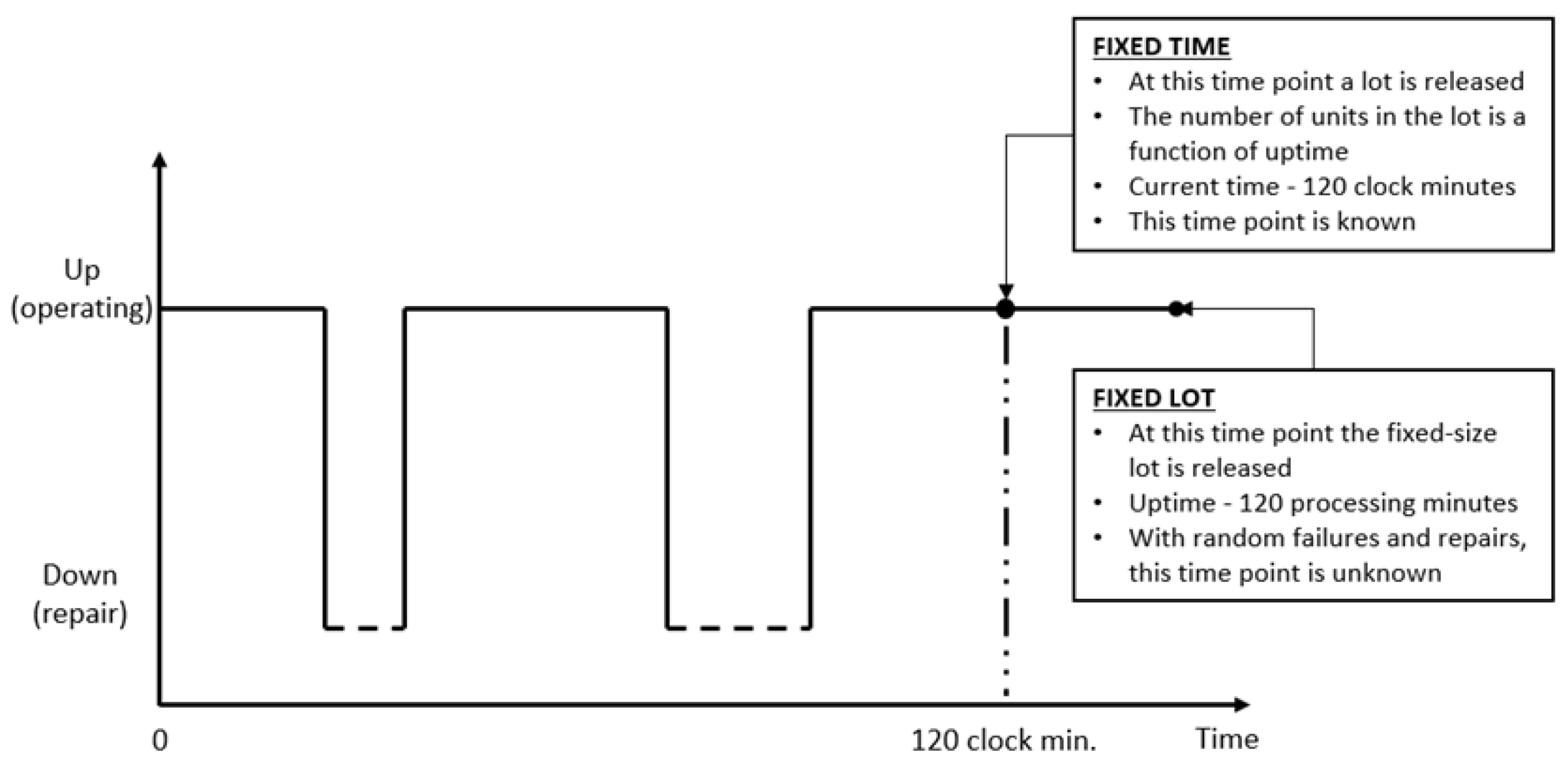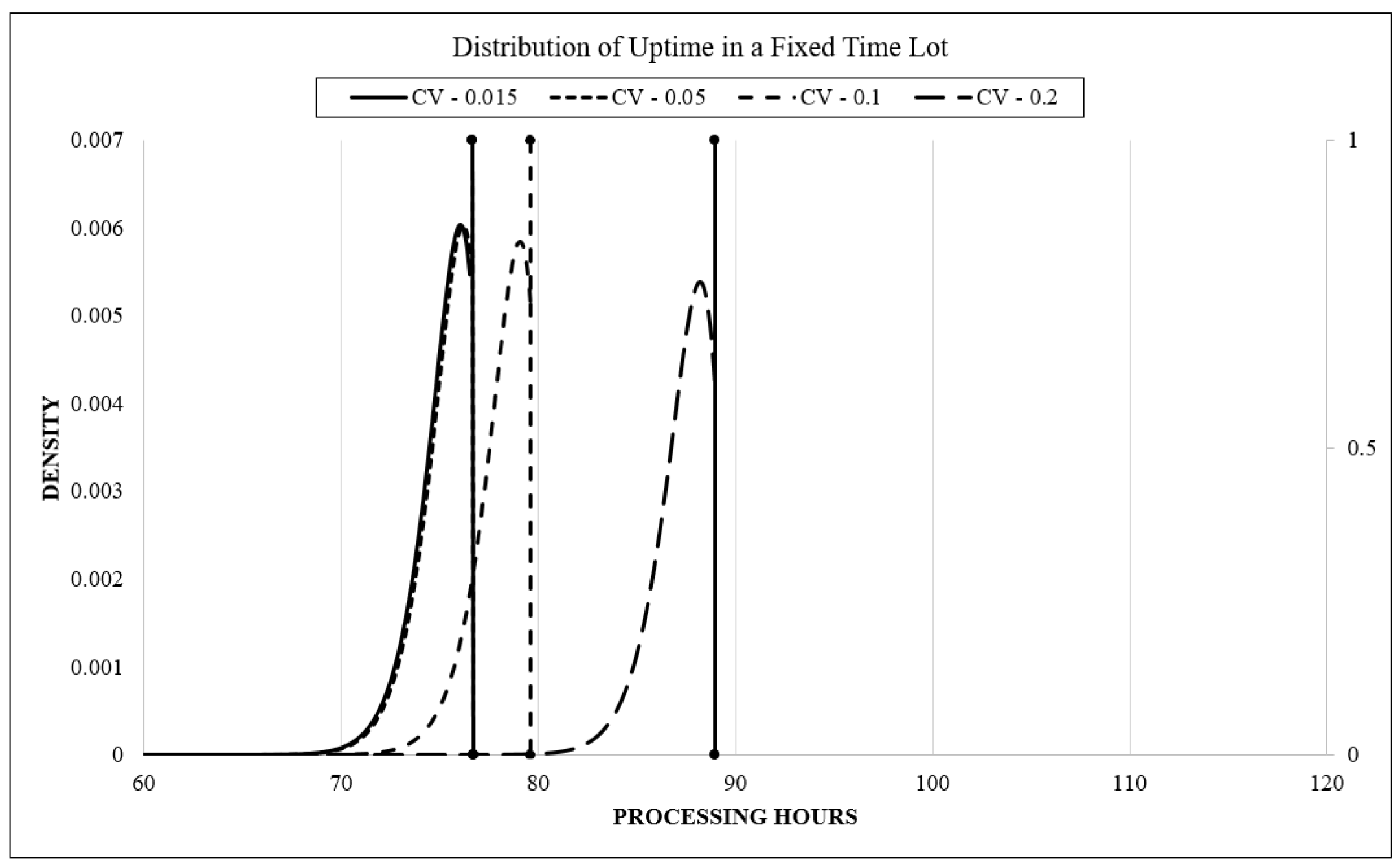When manufacturing a group of items, if the workstation remains free from interruptions, the performance of batch systems based on either fixed quantity or fixed duration would be identical, shown in Figure 1. Specifically, the total duration required to complete a quantity-based batch is the product of individual processing time and batch quantity, whereas the total output generated in a time-based batch is determined by dividing the batch duration by the processing time for each job. Conversely, if the workstation encounters unplanned disruptions and varying repair durations, the operational behaviors and outcomes of quantity-based and duration-based batch production methods will differ notably.

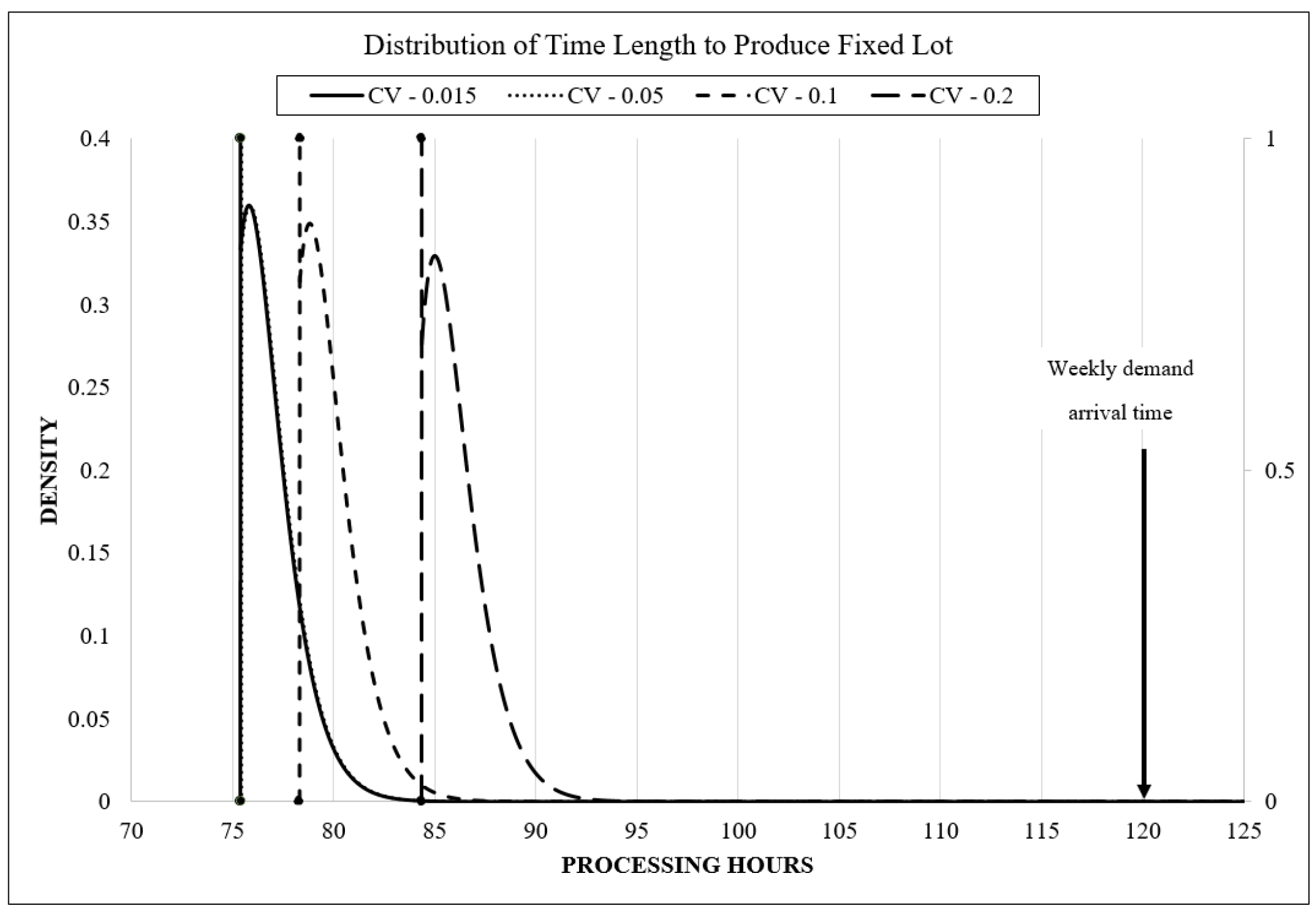
In an ideal scenario where a workstation never fails, the duration required to produce a fixed-size batch is predictable. Nonetheless, actual production environments involve unexpected interruptions occurring at uncertain intervals and lasting varying durations, introducing unpredictability into production timing (as depicted in Figure 1). Such unpredictability can cause substantial delays, complicating the scheduling and coordination of linked processes, such as assigning production times and managing setup crews. Conversely, when operating under a fixed-time system, the workstation similarly faces unplanned downtime. Unlike the quantity-based approach, production halts immediately when the predetermined duration expires, making the final number of units produced uncertain (as illustrated in Figure 1). Here, variability is transferred from the timing of batch completion to the quantity produced, creating a scenario opposite to that of fixed-quantity batch production. For an in-depth explanation of these batch production models, refer to Tiwari et al. [2].

3.1. Data

The neural network is trained using data reported by Tiwari et al. [2]. This dataset comprises a full set of experimental runs generated from a $2^k$ factorial framework, where each run represents a unique configuration of factor settings and its associated difference in long-run average cost between optimized fixed-quantity and fixed-interval batch policies. In total, cost outcomes were computed for 1536 distinct scenarios. All experimental factors and their respective levels are taken directly from Tiwari et al. [2]. Optimal batch quantities and reorder thresholds were obtained through a combination of discrete-event simulation and optimization techniques. For each experimental condition, discrete-event simulation was then applied to estimate the resulting long-run cost differential. Comparative statistical analysis classifies each scenario into one of three categories: superiority of the fixed-quantity policy, superiority of the fixed-interval policy, or absence of a statistically meaningful cost difference. Consequently, the response variable in the neural network model is defined as a three-class nominal categorical outcome. The scope of inference extends beyond the original experimental framing, since many system parameters can be translated into equivalent processing-time measures. Variables such as order size, demand uncertainty, inventory carrying charges, and shortage penalties can be reformulated in terms of production time units (e.g., minutes or hours). As an illustration, a machine with a throughput of 300 units per hour corresponds to a processing requirement of 0.2 min per unit.

Data drawn from an actual automated, high-throughput sheet metal stamping facility is applied to evaluate long-run average cost behavior under two modeling approaches: one using the original parameter units and another using parameters transformed into production-time equivalents (see

Table 2. Numerical data.

	Sheet Metal Stamping	Equivalent Time Units of Production
Demand Interarrival	120 h	120 processing hours
Machine Speed	765 JPH	60 jobs per processing hours
Demand Distribution	Log Normal	Log Normal
Demand Size	74,265 jobs	5825 p mins
Variability in Demand	8900 jobs	698 p mins
Demand CV	0.120	0.120
Mean Time Between Failures	26.37 h	26.37 processing hours
Mean Time to Repair	2.93 h	2.93 processing hours
SAA	90%	90%
Capacity utilization	90%	90%
Service Level Requirement	95%	95%
Inventory Holding Cost	0.5 ($/unit/month)	6.375 ($/p mins/month)
Ordering Cost ($/Order)	500	500
Optimized Reorder Point (Fixed lot system)	110,798 jobs	8690 p mins
Optimized Fixed-Size Lot	45,529 jobs	3571 p mins
Fixed Lot Inventory level	33,901.47	33,894.17
Fixed Lot Ordering Cost	3244.47	3244.59
Optimized Reorder Point (Fixed time system)	80,964 jobs	6349 p mins
Optimized Fixed-Time Lot	59.10 h	59.10 processing h
Fixed Time Inventory level	31,059.91	31,053.30
Fixed Time Ordering Cost	3632.87	3633.71

). Key variables—including order demand, demand variability, batch quantity, reorder threshold, and inventory carrying cost—are translated into equivalent processing-time measures based on the workstation’s operating speed (60/765 min per job). Each representation of the system is independently optimized to determine the optimal fixed-quantity batch size (Q), reorder point (r), and fixed review interval (T). Following optimization, the decision variables from the original-unit model can be directly compared with the corresponding time-based parameters of the converted model, as shown in Table 2. When the optimized values from the original formulation are converted into processing-time units, they closely align with those obtained from the time-based model. For instance, an optimal batch size of 45,229 jobs in the original system corresponds to approximately 3571 processing minutes when converted (45,229 × 60/765), which is nearly identical to the optimized batch duration derived in the converted framework. Moreover, statistical testing indicates no significant difference between the holding and ordering costs calculated under the two system representations.

This paper defines its inference space carefully to ensure broad applicability to real-world high-volume batch production systems. Factors affecting long-run average cost were selected based on the literature review and expert input, with values representing typical industry conditions. Stand-alone availability (SAA) levels of 90% and 80% reflect realistic operating performance, while MTBF values of 10 and 20 h represent typical failure frequencies [2]. Demand is modeled with daily and weekly interarrival times using log-normal distributions with controlled variability. Capacity utilization near 0.8 and cost parameters, including inventory holding, ordering, and backordering costs, are selected to align with established empirical studies.

3.2. Neural Network Architecture and Training

Uncovering how multiple system inputs jointly influence production performance can yield important managerial insights, yet deriving these relationships is inherently difficult due to their nonlinear and interdependent nature. Artificial neural networks are particularly effective in handling such complexity, as they can process numerous variables in parallel while learning the underlying cause–effect structures. In addition to their predictive capability, neural networks offer interpretive value by indicating the relative influence of individual input variables.

To analyze the observed relationships in the fixed-time and fixed-quantity experimental data, this study employs a feedforward neural network with a single hidden layer trained using the backpropagation algorithm. The structure of NN model consists of three layers—input, hidden, and output—each populated with an appropriate number of artificial neurons. The input layer contains one neuron for each explanatory variable in the dataset. The size of the hidden layer is selected through an iterative trial-and-error process, while the dimensions of the input and output layers are dictated by the nature of the problem. In this application, the output layer includes three neurons representing the possible categorical results: superior performance of fixed-quantity batches, superior performance of fixed-interval batches, or no statistically meaningful difference in cost.

All input variables are rescaled to lie within the [0, 1] interval to maintain consistency and prevent any single variable from dominating the learning process. Weighted connections link neurons across adjacent layers. Each input neuron is multiplied by its associated weights and aggregated to generate the input signal for neurons in the hidden layer, after which the resulting values are mapped back into the [0, 1] range. This mapping is achieved using a standard nonlinear activation function, most commonly the sigmoid (logistic) function. Bias nodes are incorporated into both the hidden and output layers to improve model flexibility. The same weighted-sum and activation procedure is repeated as signals propagate from the hidden layer to the output layer, defining the feedforward nature of the network. In this context, $W_{ij}$ represents the weight connecting the $i$-th neuron of one layer to the $j$-th neuron of the next layer.

Backpropagation is a training method used to adjust the connection weights in a multilayer feedforward neural network. During backpropagation, the weights and biases between input → hidden → output layers are modified to minimize the difference between the predicted output and the actual target output. This process is repeated iteratively along with the forward pass until the error is reduced to an acceptable level. The final adjusted connection weights are then used to compute the network output.

3.3. Connection Weight Approach

Once the neural network achieves acceptable prediction accuracy, the next step is to determine the relative contribution of each input factor. This is assessed by examining the magnitude and direction of the inter-neuron connection weights. Positive connection weights increase the predicted response value, while negative connection weights decrease it.

The connection weight approach has been applied in ecological and geological research; however, a review of the literature indicates that it has not been widely used in operations research. In this method, the influence of each input is calculated by multiplying the weights connecting the input to the hidden layers and the hidden to the output layers, then summing these products across all hidden nodes. To quantify the influence of each input, its absolute contribution is divided by the total sum of all absolute contributions. It produces a percentage that represents its relative significance. Input factors with larger connection weights have a greater effect on the predicted response than those with smaller connection weights. The relationship between inputs and outputs is interpreted in two steps. When both input-to-hidden and hidden-to-output weights have the same sign (both positive or both negative), the input has a directly proportional effect on the outcome. Conversely, if one set of weights is positive and the other is negative, the input factor has an inverse relationship with the outcome.

The connection weight approach is used to identify the factors with the highest relative importance in predicting the three outcomes in the experimental dataset. The results and their analysis are presented in the following section.

3.4. SHAP Analysis

To complement the connection weight approach and enhance transparency through axiomatic foundations, we employ SHAP (SHapley Additive exPlanations) analysis [27]. SHAP is one of XAI techniques to increase AI transparency [28]. SHAP values are obtained from cooperative game theory and satisfy three desirable properties: local accuracy (the sum of SHAP values equals the prediction difference from baseline), missingness (features absent from the model receive zero attribution), and consistency (if a feature’s marginal contribution increases, its SHAP value cannot decrease).

For multi-class classification problems, SHAP computes feature attributions for each output class independently. We utilize the Kernel SHAP implementation, which is model-agnostic and applicable to any black-box model, including neural networks. The background dataset for SHAP computations is constructed using k-means clustering (k = 50) of the training data to ensure representative sampling of the input space while maintaining computational efficiency.

SHAP analysis enables three forms of interpretation: (1) summary plots showing feature importance rankings with directional effects, (2) dependence plots revealing non-linear relationships between individual features and model outputs, and (3) interaction analysis quantifying how features jointly influence predictions. These visualizations directly address limitations of the connection weight approach by capturing nonlinear dependencies and feature interactions that linear weight aggregation may not fully represent.

4. Results

The proposed neural network framework is employed to study how system inputs maps to performance outcomes under two inventory control settings: lost sales and backordering.

4.1. Lost Sales Policy

A feedforward neural network configured with a 9–9–3 structure—comprising nine input nodes, nine hidden nodes, and three output nodes—was constructed for this analysis. Training parameters, including the learning rate and number of training iterations, were selected empirically. The final model was trained over 1000 epochs using a learning rate of 0.1. Model effectiveness was evaluated based on classification accuracy using randomly sampled test observations, yielding an average accuracy of roughly 85%.

Figure 2 displays the calculated importance of each input variable using the connection weight method. Positive contributions (direct relationships) are indicated by solid bars, while negative contributions (inverse relationships) are shown using patterned bars. Among all variables, the coefficient of variation (CV) of demand emerges as the most influential factor across the three possible outcomes. Its effect differs substantially across outcomes: it has a negative association with Outcome 1 and a positive association with Outcome 2. This pattern implies that as demand variability increases, fixed-time batch policies become more favorable.

The second most influential variable is stand-alone availability (SAA). For clarity and consistency, this study uses the term stand-alone availability (SAA) to describe the long-run fraction of time that a workstation is operational and capable of processing jobs, independent of upstream or downstream system interactions. SAA is computed as the ratio of mean time between failures (MTBF) to the sum of MTBF and mean time to repair (MTTR). In some manufacturing contexts, similar measures are referred to as modular availability, reflecting the availability of an individual machine module within a larger system. In this paper, these terms are treated as equivalent, and stand-alone availability (SAA) is used consistently throughout to avoid ambiguity. This clarification ensures that availability effects are interpreted as intrinsic machine reliability characteristics rather than system-level performance measures. As illustrated in Figure 2, higher SAA levels favor fixed-quantity batch policies. To further explore the combined impact of demand variability and SAA on system preference, additional intermediate levels of both factors were introduced and analyzed through simulation. For each combination, the decision variables—batch size (Q), reorder point (r), and review interval (T)—were re-optimized. Because the remaining factors contribute less to outcome prediction, their values were held constant. Figure 3 presents the resulting long-run average cost comparisons for the optimized systems across varying CV of demand and SAA levels.

At perfect availability (100% SAA), both policies yield equivalent performance. As availability declines, however, cost differences become evident. Under conditions of low demand variability and high availability, fixed-size batching achieves lower costs. In contrast, as availability decreases, fixed-time batching becomes more cost-effective. When demand variability is high and availability remains high, neither policy demonstrates a statistically significant advantage. The shaded regions in Figure 3 indicate which policy dominates or whether their performances are indistinguishable. Fixed-quantity batching is preferred when availability is high and demand variability is low. Notably, once SAA falls below approximately 85%, the fixed-lot system experiences a sharp escalation in long-run cost—visible as pronounced inflection points in the plots. This escalation stems from increased variability in fixed-lot production time caused by longer repair durations associated with reduced availability. When availability drops below 80%, fixed-time batching consistently outperforms fixed-lot batching across all levels of demand variability. The following analyses clarify the drivers behind these observations.

Figure 4 and Figure 5 illustrate mixed mass–density distributions for (i) the time required to complete a fixed-size batch and (ii) the uptime achieved during a fixed-time batch, respectively, assuming a workstation availability of 98% (MTBF = 30 h, MTTR = 0.61224 h). These distributions are shown for several demand CV levels under weekly demand cycles equivalent to 120 processing hours. As demand variability increases from 0.015 to 0.2, the optimal fixed-lot size (in processing minutes) increases to hedge against uncertainty. At this high availability level, variability in batch completion time remains sufficiently small that the likelihood of completing production before the next demand arrival is nearly certain. This allows for lower reorder points and reduced average inventory. In contrast, for fixed-time batching (Figure 5), higher demand variability necessitates longer production intervals. Even though uptime variability is low at 98% SAA, it is nonzero, leading to higher reorder points and inventory levels to satisfy service requirements. Overall, when availability is high and fixed-lot production time variability is minimal, the system can function close to a just-in-time regime, making fixed-size batching more economical.

As a result, fixed-time batching maintains lower average inventory and cost under these conditions. In summary, when system availability is low, fixed-time batch policies generally dominate fixed-lot policies, except in cases of extremely low demand variability.

4.2. Backordering Policy

A feedforward neural network with a 10–10–3 configuration was constructed and trained for 1000 iterations using a learning rate of 0.1. When evaluated on randomly selected test samples, the model achieved an average classification accuracy of approximately 82%. The connection weight technique was applied to assess the influence of individual input variables, with the results illustrated in Figure 6. Positive contributions, indicating direct relationships, are shown with solid bars, whereas inverse relationships are represented by patterned bars. Consistent with the lost-sales setting, the coefficient of variation of demand is the most influential factor under the backordering policy, followed by stand-alone availability (SAA). In the fixed-quantity batching context, inventory holding cost also exhibits a relatively strong impact on performance outcomes.

To further examine the effects of demand variability and availability, additional levels of the CV of demand and SAA were introduced and evaluated through simulation. Because the remaining variables contribute less to outcome prediction, their values were fixed. For each new factor combination, the decision variables—batch size (Q), reorder point (r), and review interval (T)—were re-optimized.

Figure 7 and Figure 8 use boxed regions to indicate scenarios in which one policy dominates or where cost performance is statistically indistinguishable. When availability is perfect (100% SAA), both batching strategies yield comparable costs across all levels of demand variability. As availability declines, differences become more pronounced. Figure 7 shows that at low demand variability and high availability, the two systems perform similarly, whereas at lower availability levels, fixed-time batching becomes more cost-effective. At high demand variability combined with high availability, neither policy shows a clear advantage. Cost drivers in backordering case mirror those observed under lost sales.

When inventory holding costs are high, availability is high, and demand variability is low, both batching policies again exhibit similar performance (Figure 8). However, as availability decreases under low demand variability, fixed-quantity batching becomes more favorable. Conversely, at higher demand variability, the fixed-time policy outperforms the fixed-quantity approach. As in the lost-sales case, once availability drops below roughly 90%, the long-run average cost of the fixed-quantity system rises sharply. At elevated holding-cost levels, both systems favor smaller, more frequent batches. Yet increasing demand variability and declining availability necessitate higher reorder points, larger batch sizes, and greater inventory buffers. These effects disproportionately raise holding costs in fixed-quantity systems, leading to higher overall costs.

4.3. SHAP Feature Importance Validation

We applied SHAP analysis to both trained neural networks. Figure 9 presents SHAP summary plots for the lost sales and backordering policies. Features are ranked by mean absolute SHAP values, with color indicating feature magnitude (red indicates high values, blue indicates low). The horizontal position shows each observation’s SHAP value, revealing both importance and directional effects.

For the lost sales policy (Figure 9a), the coefficient of variation of demand is the most influential factor (mean |SHAP| = 0.232), consistent with the connection weight analysis. Higher demand variability (red points) strongly increases preference for fixed-time lots (positive SHAP values), while low variability favors fixed-size lots. Service level ranks second (mean |SHAP| = 0.122), followed by MTTR (0.108) and SAA (0.090). For the backordering policy (Figure 9b), SHAP analysis identifies CV of demand (mean |SHAP| = 0.155), SAA (0.149), inventory holding cost (0.145), and ordering cost (0.135) as the four most important factors. The top four features match exactly between the SHAP and connection weight rankings. Figure 10 and Figure 11 illustrate importance values by outcome class.

4.3.1. Non-Linear Relationships

SHAP dependence plots (Figure 12) reveal the functional form of feature-outcome relationships that cannot be detected solely from connection weight analysis. For CV of demand (Figure 12a,c), the relationship with fixed-time preference is monotonically increasing across both policies. The interaction coloring reveals that SAA modulates this effect: at low availability (blue points), the impact of demand variability is amplified.

The SAA dependence plots (Figure 12b,d) show a threshold effect around 85% availability, corroborating the simulation outcomes presented in Section 4.1 and Section 4.2. Below this threshold, fixed-time lots become increasingly favorable regardless of demand variability. This non-linear pattern provides additional evidence for the critical availability threshold identified in this study.

4.3.2. Feature Interactions

Figure 13 presents interaction heatmaps. Notable interactions between MTTR-MTBF and SAA-MTBF for lost sales indicate joint effects among the reliability parameters.

4.3.3. Method Validation

Table 3. Comparison of feature importance rankings.

Feature	Lost Sales		Backordering
	SHAP	CW	SHAP	CW
CV of Demand	1	1	1	1
SAA	4	2	2	2
Service Level	2	3	9	8
Inventory Holding Cost	7	4	3	3
Ordering Cost	8	6	4	4
MTTR	3	5	10	9
MTBF	9	9	7	7
Capacity Utilization	5	7	5	6
Demand Interarrival	6	8	6	5
Backordering Cost	-	-	8	10

and Figure 14 compare feature importance rankings between SHAP and the connection weight (CW) approaches. For the backordering policy, methods show near-perfect agreement (Spearman ρ = 0.952, p < 0.0001), with identical rankings for the top four features. For the lost sales policy, agreement remains strong (ρ = 0.750, p = 0.020), with both methods identifying CV of demand as the dominant factor (rank 1) and MTBF as the least important (rank 9).

The convergence of rankings across methods provides robust evidence for the identified key drivers. Minor ranking differences for mid-tier features likely reflect SHAP’s ability to capture non-linear effects that linear weight aggregation may underestimate. Both methods consistently identify demand variability and system availability as the dominant factors influencing the relative cost performance of fixed-time versus fixed-size lot production systems.

5. Discussion

The strong convergence between SHAP and connection weight rankings across both inventory policies provides additional evidence of the robustness of these results. While the connection weight approach offers computational simplicity suitable for practitioners, SHAP provides axiomatic foundations and the ability to detect nonlinear relationships and interaction effects. The near-perfect correlation (ρ = 0.952) between the backordering policy and the simpler connection weight method demonstrates that the latter effectively captures the same information as game-theoretic attribution methods in this application domain. The consistency across methods strengthens confidence in the practical recommendations derived from this analysis.

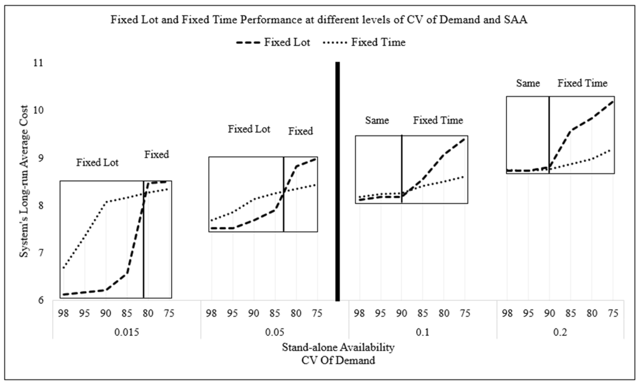
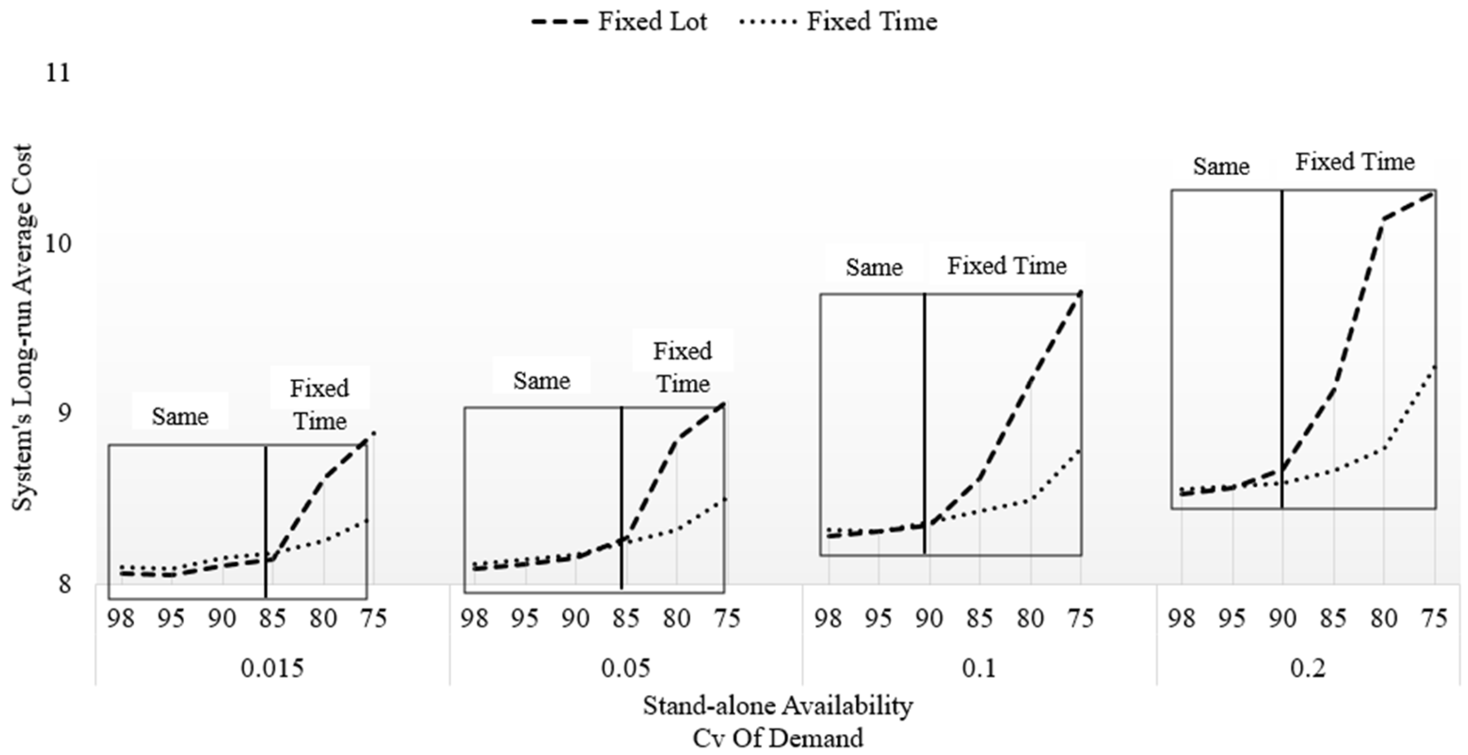
The feedforward neural network (FFNN) applied in this study reveals meaningful patterns regarding the performance of fixed-size lot and fixed-time lot batch production systems. The findings highlight the critical influence of demand variability and stand-alone availability on cost outcomes under both lost sales and backordering policies. When demand is stable and workstation availability is high, fixed-size lot systems operate more efficiently by enabling just-in-time production with minimal inventory. However, as availability declines and demand variability increases, the fixed-time lot system becomes more cost-effective due to its ability to maintain service levels without excessive inventory buildup. The FFNN’s connection weight analysis not only confirms these relationships but also quantifies the relative importance of each input factor, offering a granular understanding of their influence. The findings highlight a significant cost tradeoff threshold around 85% availability, where the cost advantage shifts from fixed-size to fixed-time production. This research demonstrates that fixed-time lot systems, though less common in industry, may offer substantial benefits under specific operational conditions. These insights can guide production managers in selecting appropriate control systems based on key operational parameters, enabling more agile and cost-efficient decision-making in complex manufacturing environments.

5.1. Managerial Implications

From a business analytics perspective, the proposed neural-network framework is well suited for deployment as a practical decision support system in modern manufacturing environments. Key input variables such as stand-alone availability (SAA), mean time between failures (MTBF), and mean time to repair (MTTR) are routinely captured in real time through manufacturing execution systems (MES), computerized maintenance management systems (CMMS), and industrial IoT sensors that monitor machine states, downtime events, and repair durations. Demand rates and variability are similarly available from enterprise resource planning (ERP) and order management systems. Once trained offline using historical or simulated data, the neural network can be embedded as a lightweight decision layer that evaluates current operating conditions and recommends the preferred batching policy without requiring re-optimization. Because the model relies on normalized inputs and categorical outputs, it supports rapid online inference and can be updated periodically using rolling data windows to reflect changes in demand patterns, reliability, or cost structures. This enables managers to monitor proximity to critical thresholds—such as the identified ≈85% availability tipping point—and proactively switch production control policies before cost performance deteriorates. In this way, the model functions not as a static analytical tool, but as a prescriptive analytics component that integrates seamlessly with existing digital manufacturing infrastructures to support real-time, data-driven operational decisions.

The insights generated by this study are applicable to a broader set of manufacturing settings that fall within the same experimental domain, provided system parameters are first transformed into comparable production-time measures. In this way, the results offer practical direction for manufacturing decision makers. The analysis demonstrates that demand variability, measured by the coefficient of variation, and workstation stand-alone availability play a decisive role in determining the relative effectiveness of the two production control policies. When equipment availability is high, conditions are favorable for just-in-time operation: completed portions of fixed-quantity batches are consistently available before demand occurs, enabling customer requirements to be met with minimal inventory and without excessive shortages. In contrast, when availability deteriorates and demand becomes more volatile, batch completion is frequently delayed beyond demand occurrences, forcing firms to carry larger inventory buffers to control shortages or backorders.

As an illustration, consider a workstation governed by a fixed-quantity batching rule in which material handling is scheduled around completed batches. If production delays become common and partially completed batches must be rushed through the system to prevent unmet demand, this behavior signals inefficiency under the current policy and suggests that a time-based batching approach may offer a lower-cost short-term alternative. In general, when variability in batch completion time increases because of reduced equipment availability, time-based production control tends to yield superior long-run cost performance. Conversely, improvements in workstation availability may justify a shift back toward quantity-based batching.

Despite these potential advantages, time-based batching is seldom implemented in industrial practice. The findings suggest that it can outperform quantity-based control under specific operating conditions, yet several factors help explain its limited adoption. Many high-throughput manufacturing environments have gradually evolved toward stable demand patterns and highly reliable equipment, conditions that naturally favor fixed-quantity policies. In addition, time-based production introduces uncertainty into materials planning, handling operations, and inventory storage, complicating managerial decisions related to raw-material procurement, handling capacity, and space requirements. For instance, stamping operations often rely on specialized containers designed to hold a fixed number of parts; these containers are costly and space-intensive, making predictable fill levels important. Moreover, time-based batching may be unsuitable for products involving perishable or non-returnable materials, such as tire compounds, automotive paint mixtures, pharmaceutical inputs, or chemicals requiring controlled storage environments. Lastly, the scarcity of published studies and industrial examples involving time-based batch control has limited its visibility and acceptance as a viable alternative in manufacturing practice.

5.2. Limitations and Future Research

The primary advantage of the proposed approach lies in its ability to capture complex, nonlinear relationships among demand variability, machine reliability, and cost parameters without imposing restrictive functional assumptions. When combined with explainability tools such as connection weight analysis and SHAP, the framework yields interpretable, outcome-specific insights that support prescriptive decision making. Moreover, the method is computationally efficient at the inference stage, making it suitable for integration into decision support systems. However, the approach also has limitations. Neural networks require representative training data and careful validation to avoid overfitting, and the resulting insights are bounded by the experimental domain used for training. Unlike closed-form analytical models, the method does not yield explicit mathematical expressions for optimal policies, which may limit its use in highly stylized theoretical analyses. As such, the proposed framework should be viewed as a complementary decision-support tool that augments, rather than replaces, traditional analytical and optimization-based methods in production and inventory research.

While the results highlight the effectiveness of fixed-time lot systems under specific combinations of demand variability and machine availability, several assumptions should be acknowledged when interpreting their generalizability. First, the analysis is based on a single-item production system operated on a stand-alone workstation without sequence-dependent setups or product changeovers. Although many high-volume manufacturing environments approximate this structure, multi-product and multi-machine systems may exhibit additional dynamics that alter policy tradeoffs. Second, the neural network is trained on data generated within a predefined experimental domain reflecting typical industrial ranges for demand, reliability, and cost parameters. Consequently, predictions and policy recommendations are most reliable within this domain and should be recalibrated if applied to substantially different operating conditions. Third, the study focuses on long-run average cost as the primary performance metric; other objectives such as service differentiation, sustainability, or workforce constraints may lead to different policy preferences. Finally, although the explainable neural-network framework mitigates black-box concerns, it does not yield closed-form analytical expressions, which may limit its use in highly stylized theoretical settings. These considerations suggest that the proposed framework is best viewed as a prescriptive decision-support tool whose insights complement, rather than universally replace, traditional analytical approaches.

6. Conclusions

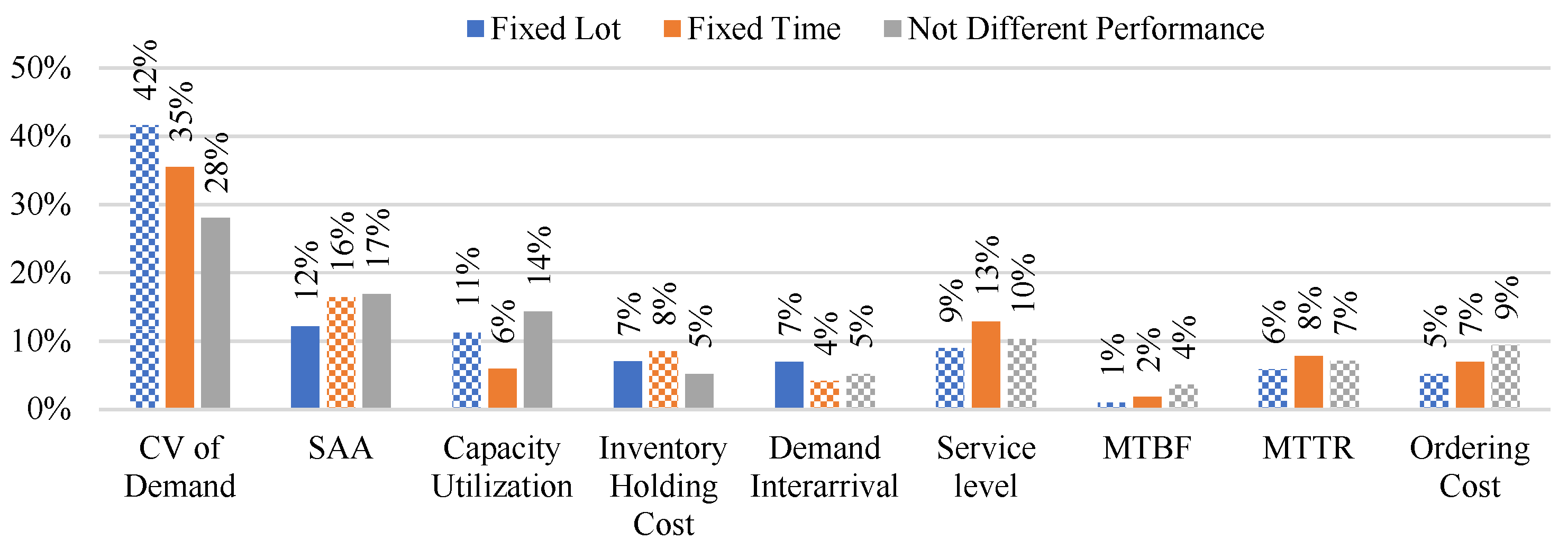
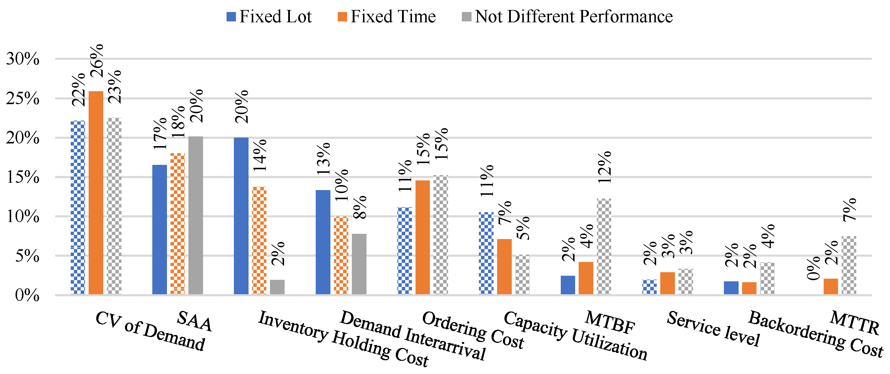
This research evaluated experimental outcomes from two alternative batch production control strategies in order to uncover the relationships between system inputs and discrete performance classifications. By doing so, it offers clearer insight into the conditions under which fixed-quantity or time-based batching is likely to be more effective. The conclusions drawn from the feedforward neural network analysis are not limited to the specific system studied but also apply to other production systems that reside within the same experimental domain. The feedforward neural network, combined with the connection weight technique, is employed to develop a predictive model for three distinct scenarios: (1) when the fixed-quantity batch system outperforms in cost, (2) when the fixed-duration batch system shows superior cost performance, and (3) when both systems yield comparable costs. The influence and polarity of the weight values between layers are analyzed to determine the significance of each input variable in predicting these outcomes. Results indicate that, under a lost sales framework, the most influential parameters are the demand variability (measured by coefficient of variation) and the workstation’s operational uptime. In contrast, when backorders are allowed, the timing between customer demands, system uptime, and inventory expenses emerge as the most critical variables.

The response variable in this study is formulated as a three-class categorical outcome—fixed-size better, fixed-time better, or no statistically significant difference—rather than a continuous cost difference. This formulation reflects the managerial reality that policy changes are typically justified only when cost advantages are both economically meaningful and statistically robust. Although numerical cost differences exist in all scenarios, many lie within stochastic variability bands where switching policies yields no reliable benefit. By framing the problem as a classification task, the analysis focuses on identifying decision regimes, nonlinear thresholds, and dominant drivers of policy preference, rather than minimizing numerical prediction error. This perspective aligns the modeling approach with practical production control decisions made under uncertainty.

To gain deeper insight into how these factors affect system behavior, simulations were conducted using additional levels for these inputs, alongside optimized batch quantities and reorder thresholds. Under lost sales conditions, high availability and stable demand lead to reduced production variability, allowing fixed-quantity systems to function efficiently in a just-in-time fashion, thereby reducing expenses. However, as variability rises and availability drops, this efficiency deteriorates, making fixed-time systems more cost-effective.

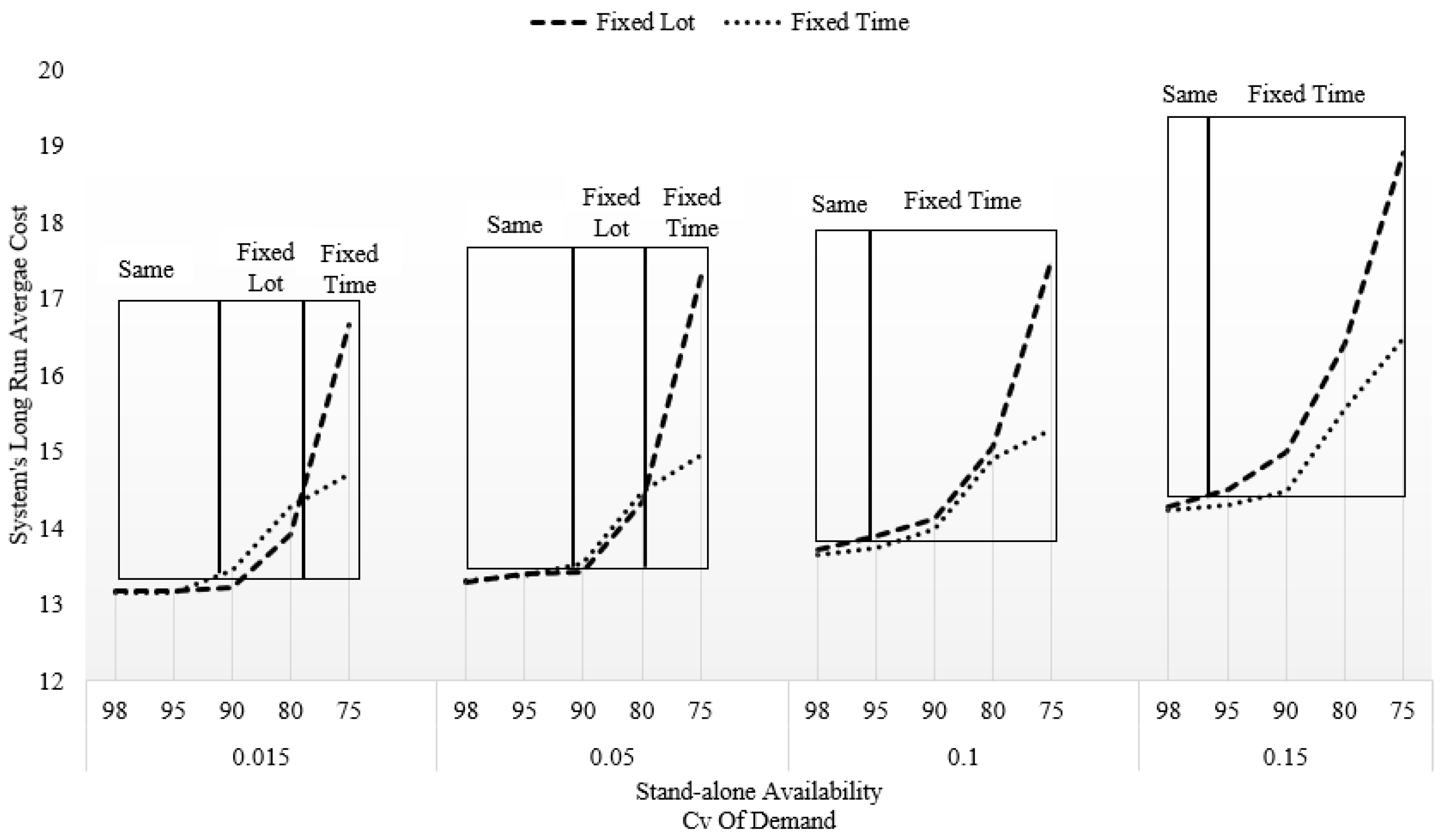
In backordering environments, similar patterns emerge. At low inventory costs, greater demand variability and reduced uptime favor the fixed-time model. When inventory holding becomes more expensive, both systems shift toward smaller, more frequent batches. Yet, fixed-quantity setups tend to build up larger stock buffers to manage uncertainty, especially when availability is low and demand fluctuates. This often results in delays in batch completion, excessive inventory buildup, and ultimately, higher operating costs for fixed-quantity systems.